A Method for Managing ADS-B Data Based on a 4D Airspace-Temporal Grid (GeoSOT-AS)

Abstract

With the exponential increase in the volume of automatic dependent surveillance-broadcast (ADS-B), and other types of air traffic control (ATC) data containing spatiotemporal attributes, it remains uncertain how to respond to immediate ATC data access within a target area. Accordingly, an original multi-level disaggregated framework for airspace, and its corresponding information management is proposed. Further, a multi-scale grid modeling and coding mapping method of airspace information represented by ADS-B is put forth. Finally, tests on the validity of the 4D airspace-temporal grid we named as the GeoSOT-AS framework were conducted across key areas based on the development of an effective data organization method for ADS-B, or an effective algorithm for extracting relevant spatiotemporal data. Experimentally, it was demonstrated that GeoSOT-AS conforms to the existing Chinese specification of civil aeronautical charting and is advantageous for its low deformation and high practicality; furthermore, the airspace grid identification code modeling was less costly, and improved performance by >80% when used for ADS-B data extraction. GeoSOT-AS can thus provide effective reference and practical information for existing airspace data management methods represented by ADS-B and can subsequently be extended to other forms of airspace management scenarios.

1. Introduction

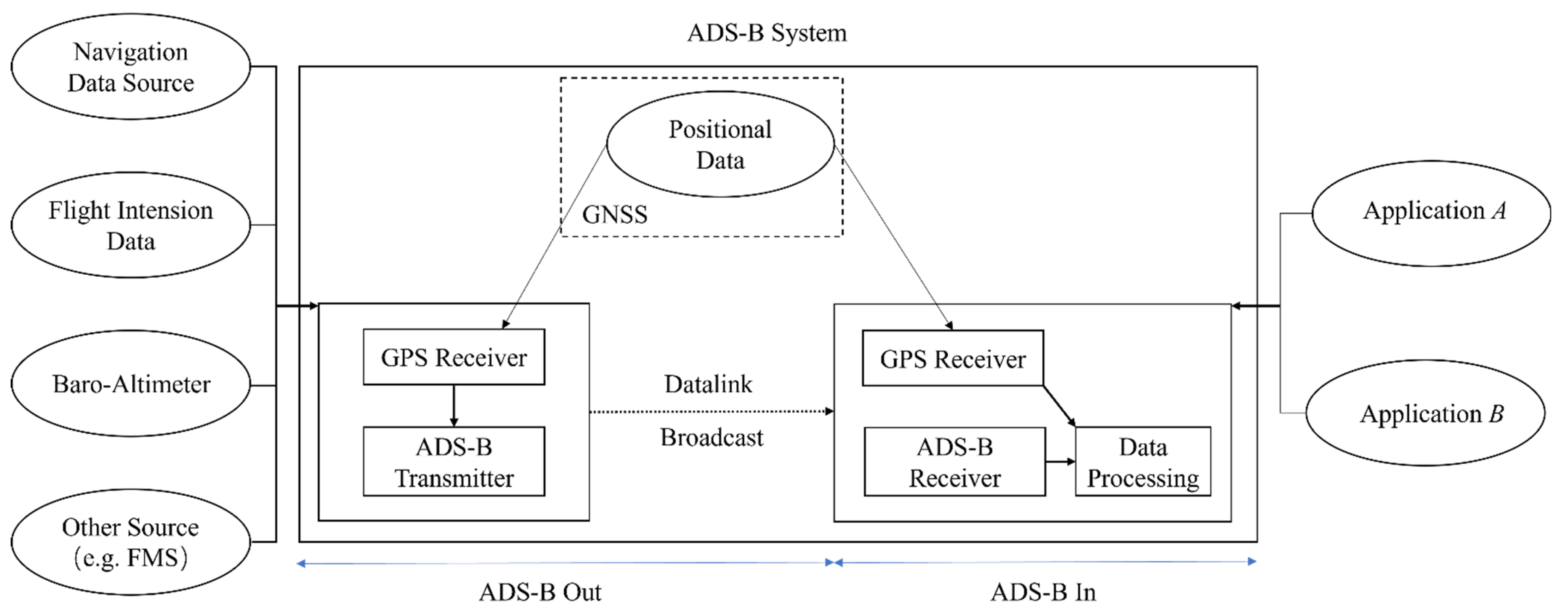
An automatic dependent surveillance-broadcast (ADS-B) system [1] is an acronym for the broadcast-type automatic correlation surveillance system, which consists of multiple ground-based and airborne stations to complete two-way communication of data in a grid, or in a multi-point to-multi-point manner. The ADS-B information system integrates communication and surveillance and consists of three parts: information source, information transmission channel, and information processing and display. The specific composition is shown in Figure 1.

ADS-B, as a new air traffic control (ATC) surveillance technology based on GPS and the use of air–ground and air–air data links for traffic monitoring and information trans-fer, is widely used across various fields. For example, when facing the consistency, ad-vantages, and shortcomings of ADS-B and GPS, Identify Friend or Foe systems (IFF) and other positioning or navigation systems are introduced [2]. A three-level collision avoidance system based on transport aviation is proposed based on ADS-B technology applied to general aviation [3]. Initial results [4], as well as a collision avoidance planning approach combining ADS-B and dynamic planning [5], proposed an overall set of system specifications for ATC coherent surveillance systems [6]; whereas this work proposes an ADS-B-based technique for the error calculation of each sensor in a fusion system using artificial intelligence techniques to understand their corresponding error profile within a geographical area and improve fusion accuracy [7]. In this context, various aspects of the research have enhanced and extended the new navigation system with a very rich set of features, as well as bringing potential challenges, in addition to socioeconomic benefits.

With the advent of big data, storage and analysis of stock ADS-B, as well as other kinds of ATC data with spatiotemporal attributes, have been explored in depth. The premise of the above application and analysis operation lies in extracting data from the whole stock database for analysis across target areas and the processing of aircraft positions over time. Although scholars have noticed this association, the traditional approach to the management of aerial information presents a fragmented state, and is to some extent limited by the influence of various data sources and corresponding qualities [8]. Indeed, different data types have led to various databases and data management methods. For example, a new compressed indexing method for managing ADS-B data has been proposed in the literature [9], the basic building blocks of which are spatiotemporal reference partitioning, reordering, and compression. Similarly, there is a compressed storage method for 4D air traffic trajectories [10], as well as the development of an airport navigation service database based on GIS tools, and other notable methods [11]. Under such conditions, ATC flight data exists only in corresponding file databases with their own file management methods, which do not co-align with actual airspace, and cannot quickly respond to the immediate availability of ATC data within a target area.

Simultaneously, digitalization and intelligence are becoming the focus of competition in the fourth global industrial revolution [12]. In the context of digital airspace, its management includes not only that of flight space, but internal element information as well, such as basic navigation data, occupancy status, etc. Combining the management of airspace with that of correlated information represented by ADS-B data can comprise a novel applicable data management method [13,14]; thus, as the management of ATC data is ultimately for flight services, the method of airspace management can be applied to that of ATC data to achieve a direct data mapping of airspace. According to the ATC access requirements for aircraft flights, different types of airspace are subdivided for targeted operational management and control. The representative ones are divided into two main categories: a class of airspace segmentation and configuration methods based on terminal areas or flight requirements. Existing methodologies include dynamic airspace sector segmentation based on V-maps [15]; whereas Tang et al. [16] proposed similar segmentation based on geometric models, leading to the development of new dynamic airspace configuration algorithms, such as those based on graph theory [17], and dynamic airspace configuration based on genetic dynamic airspace configuration algorithms [18]. Another type of airspace classification method is oriented towards the delineation of airway routes, such as the dynamic airspace super sectors (DASS) concept-based airway airspace design and operation scheme [19], as well as the high-volume tube-shape sectors (HTS) prototype concept [20], in addition to the combination of a district airspace and new freeway airspace [21].

In general, the traditional airspace management based on density, traffic, route delineation, and other paradigms are not compatible with the chart system, nor with the actual flight chart display needs to conduct the multitude of required calculations and conversions; thus, it remains unsuitable for the ATC data management framework oriented to ADS-B as a representative data source. It is hoped that the management of flight data and airspace can be directly combined for navigation services, where the most direct guidance for flight services being the chart standard [22].

The present study proposes a discrete digital airspace framework, GeoSOT-AS, for control purposes. The framework conforms to the existing Chinese specification of civil aeronautical charting. It uses a specific space-filling curve approach, has good inheritance between multi-level profiles, and is characterized by low deformation and high practical-ty. The framework is validated by calculations in majority of the Chinese airspace and is identified by a unique code for each unique airspace location, which can also be used as the main key for database management of ATC information. The system performed well in extracting target airspace area data, such as ADS-B data extraction tasks, improving the overall extraction rate by ≥80% compared to traditional range queries. The GeoSOT-AS grid framework can be used for basic airspace management tasks, such as regional trajectory clustering studies, collision avoidance, airspace planning, and deployment. By matching the framework with the chart, the results of regional analyses can be quickly applied to actual airspace management. As a digital framework for multi-level disaggregation, this framework can carry air traffic data for aviation tasks and provide an effective reference for existing airspace management methods.

2. Related Work

Research on the data management of ADS-B is limited, but this problem is consistent with the management and use of aviation big data in related fields. Therefore, we present some related work that specifically includes database storage methods, column storage methods, and point-based spatiotemporal indexing methods, among others.

Traditional database storage methods, such as Google’s Bigtable [23], are based on an ordered multi-table structure, and the use of keywords and timestamps for queries. The principle is similar to the GAE DataStore [24], which was one of the earliest systems to use the idea of spatial dissection. In addition, there are general-purpose distributed frameworks based on the Hadoop [25] and Spark system [26]. On the other hand, the general idea of column-based storage [27] has a long tradition in data processing, such as MonetDB [28], and is now commonly used in the current storage database; however, these databases are not well adapted to the embedding and querying of other field parameters of the document.

Similarly, point-based spatiotemporal indexing methods are mainly divided into two categories: spatiotemporal separated indexing and spatiotemporal integrated indexing. The former category includes many tree structures in GIS tools that are typical representatives, which can only use indexes in the spatial dimension and can only filter in the temporal dimension. Examples include Quad-tree [29], Quad-tree + Inverted Index [30], R-tree [31], and Partial Local Quad-tree [32]. These indexing methods may experience a significant decrease in query efficiency when dealing with problems such as spatiotemporal applications, especially with the influence of the query situation and conditions. In contrast, the latter category includes tree-based spatiotemporal indexes, which directly transform traditional spatial data into spatiotemporal indexes by combining time more easily. Examples of this category include CloST (Hierarchical quad-tree) [33], Elite (Oct-tree) [34], and grid-based spatiotemporal indexes by combining the grid and Space Fill Curve (SFC) such as Z-curve [35] and Hillbert-curve [36] to convert multiple dimensions of space and time into one-dimensional dictionary indexes. Examples of this include CoPST (SFC) [37] and GeoMesa (Geohash + SFC) [38]. However, the blockiness, readability, and identifiability of the grid are not incorporated into the practical use in these cases.

Based on the considerations mentioned above, we have selected the document-based database MongoDB for experimental operations. This database allows for the retention of certain parameters of ADS-B, such as takeoff and landing airport heading angles, in the form of JSON data. We have used the grid indexing method, considering that the grid profile is compatible with the flight chart. The resulting grid code has the characteristics of both indexing primary key and position identification. Furthermore, this method decouples the altitude and time dimensions to improve efficiency, and this performs well in extracting the ADS-B data in the target airspace.

3. A 4D Airspace-Temporal Grid Framework (GeoSOT-AS) for ADS-B Data Organization

The 2ⁿ one-dimensional integer global subdivision grid with one-dimension-integer on two to nth power (GeoSOT) [39] proposed by the Peking University team is a latitude and longitude subdivision grid system. GeoSOT subdivision grids and codes are advantageous for their global uniqueness, multiscale, and flexible extension, etc. The grid codes are controlled by the number of bits [40], which are sufficient to accurately represent spatial information of arbitrary location and size, while maintaining characteristics of small deformation, multiscale, simple subdivision, rapid computational processing, etc., and are used in a variety of spatial information organization fields [41].

This section investigates the application of the earth segmentation principle corresponding to the Chinese specification of civil aeronautical charting. Meanwhile we try to reshape the airspace grid coding model and establish the airspace spatial location coding identification system and aims to form a discrete grid framework designed for air traffic management, ADS-B, and other kinds of flight information elements. The redesigned airspace grid segmentation and coding methods must adhere to the following requirements:

• Partial grid flattening: For large aircraft with fast flight speeds in the horizontal direction and slow climbing speeds, the grid must be switched flexibly according to the specific application requirements and cannot be strictly polygonal. Therefore, during design, the height and planar dimensional grids are decoupled and treated independently;
• Code identification uniqueness: One identification code corresponds to only one grid under the same hierarchy;
• The height required to reach adjacent space.

In response to the above constraints, based on the original GeoSOT geo-profile method, and in line with the Chinese specification of civil aeronautical charting, the profile method was redrawn to make it applicable to airspace element information management, while accounting for the temporal dimension. The airspace grid coding model was defined in the airspace based on latitude and longitude coordinates by treating the plane and altitude dimensions, as well as the time dimension separately in an approach termed here as GeoSOT-AS (airspace), a multi-level 4D airspace-temporal grid framework for the ADS-B data organization.

GeoSOT-AS has been designed with a spatial plane, altitude, and a temporal dimension, resulting in a decadal dissection in the latitude and longitude directions, extending from degree to second level regions, a multiscale division in the altitude direction from a base 150 m stratification to the adjacent space (covering the base flight altitude stratification), and a temporal dimension (days to seconds), with each of these three elements described by specific codes. In the GeoSOT-AS architecture, any moment in time in the Earth’s airspace can be expressed by the following Equation (1):

(1)

where P, H, and T represent discrete codes in profile form; and $f_i$,$f_j$,$f_k$ correspond to the specific conversion forms and coding methods for latitude, longitude, altitude and time of the plane, respectively. The specific coding design conversion and coding methods are described below.

3.1. GeoSOT-AS Rules and Methods for Planar Dimensional Profiling

3.1.1. Planar Dimensional Profiling Method

Considering the above three practical needs of actual airspace and flight information management, it has been proposed that the profile of the earth’s surface plane corresponds to the multi-level Chinese specification of civil aeronautical charting, with a base consideration design which can be compatible with various tasks of airspace data management (Figure 2).

The chart correspondence constraints are as follows:

• Aeronautical charts, which are those used by aircraft for flight paths or routes and can cover a large area, generally maintain a scale of 1:1,000,000, corresponding to the first level of GeoSOT-AS sectional charts;
• Regional charts, which are generally enlarged charts of flight paths in areas of intense flight activity and complex airspace, are generally at a scale of 1:500,000, and correspond to the second level of GeoSOT-AS;
• Terminal area charts (TACs), such as airport plans, parking space, standard approach and departure, instrument approach, fuel discharge area, airport obstacle, and air corridor charts, are at scales of 1:250,000, corresponding to the third level of GeoSOT-AS (

  Table 1. GeoSOT-AS planar dimensional dissection scales corresponding to multi-level charts.

  Level	Planar Scale	Approximate Size Near Equator	Aerial Chart Size	Proportion
  1	6° × 4°	\	6° × 4°	1:1,000,000
  2	3° × 2°	\	3° × 2°	1:500,000
  3	1° × 1°	111.32 km	1°30′ × 1°	1:250,000
  4	30′ × 30′	55.66 km	30′ × 20′	1:100,000
  5	15′ × 10	27.83 km	15′ × 10′	1:50,000
  6	5′ × 5	9.28 km	\	\
  7	1′ × 1′	1.86 km	\	\
  8	30″ × 30″	928 m	\	\
  9	15″ × 15″	464 m	\	\
  10	5″ × 5″	154.6 m	\	\
  11	1″ × 1″	31 m	\	\

  shows the specific correspondence);
• Such forms are compatible with all kinds of finer scale maps, including major areas, with 100 km, 1 km level, and 100 m level granularity.

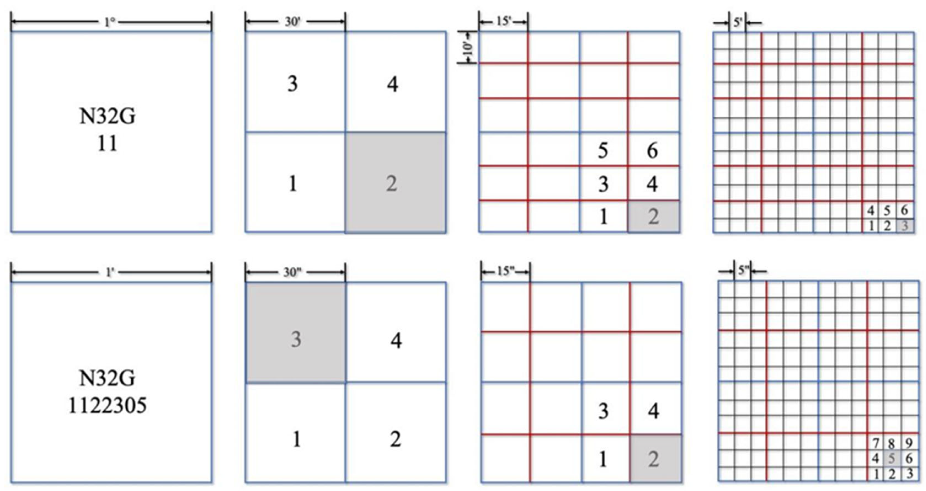
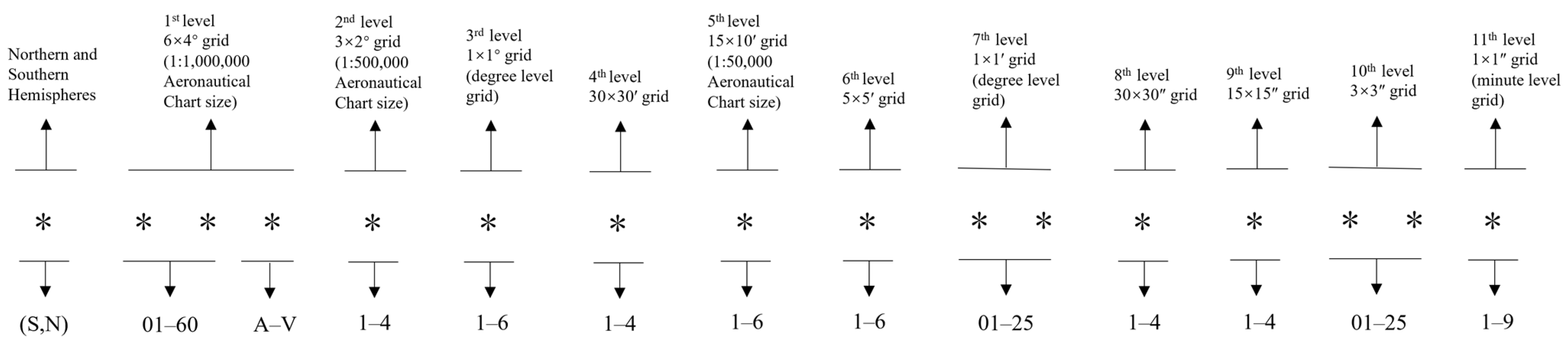
Based on the above constraints and correspondences, the following airspace planar dimensional discretization was designed, with the basic discretization architecture shown in Figure 3. The origin of the Earth’s surface airspace 2D grid is at the intersection of the equator and the prime meridian. The Earth’s surface 2D grid is divided into 11 levels according to the following division method:

The 1st-level grid is divided according to the 1:1 million aeronautical chart, with a cell size of 6° × 4°, and is used as the basic framework for the national airspace management.

The 2nd-level grid is divided according to the 1:500,000 aeronautical chart, with a cell size of 3° × 2°.

The 3rd-level grid is divided into 3 × 2 s-level grids according to the equal division of latitude and longitude, corresponding to a 1° × 1° grid (~111.32 × 111.32 km) at the Earth’s equator. This corresponds to a 100 km level grid.

The 4th-level grid is divided into 2 × 2 according to latitude and longitude equalization, corresponding to a 30′ × 30′ grid (~55.66 × 55.66 km at the Earth’s equator).

The 5th-level grid is divided into 2 × 3 grids according to latitude and longitude equalization, corresponding to a 15′ × 10′ grid of 1:50,000 aeronautical chart area (~27.83 × 18.55 km at the Earth’s equator).

The 6th-level grid is divided into 3 × 2 grids according to 5′ × 5′ latitude and longitude (~9.28 × 9.28 km at the Earth’s equator).

The 7th-level grid division is divided equally by latitude and longitude into 5 × 5 grids corresponding to 1′ × 1′ (~1.86 × 1.86 km at the Earth’s equator).

The 8th-level grid is divided into 2 × 2 grids, corresponding to 30″ × 30″ grid (~928 × 928 m grid at the Earth’s equator), according to latitude and longitude equalization.

The 9th-level grid is divided into 2 × 2 grids, corresponding to 15″ × 15″ (~464 × 464 m at the Earth’s equator), according to equal divisions of latitude and longitude.

The 10th-level grid is divided equally by latitude and longitude into 3 × 3 grids, corresponding to 5″ × 5″ (~154.6 × 154.6 m at the Earth’s equator).

The 11th-level grid is divided into 5 × 5 according to latitude and longitude, corresponding to a 1″ × 1″ grid (~31 × 31 m at the Earth’s equator).

The profiling method is compatible with the Chinese specification of civil aeronautical charting at multiple levels, showing good inheritance and compatibility between multiple map levels (Table 1); thus, it provides a solid basic framework for existing ADS-B data management.

3.1.2. Planar Dimensional Coding Method

Definition 1. 

Primary dissection blocks are those above the degree level of dissection, applicable to aeronautical plans at scales of 1:250,000 and above and corresponding to the first three levels of dissection in Table 1.

Definition 2. 

Secondary sectioning blocks are the eight levels of sectioning below the degree level, for aerial plans at scales of 1:100,000 and below.

The following coding methods from each of the two are described as follows, adapted to their method of dissection:

(a)

Coding method for primary profile blocks.

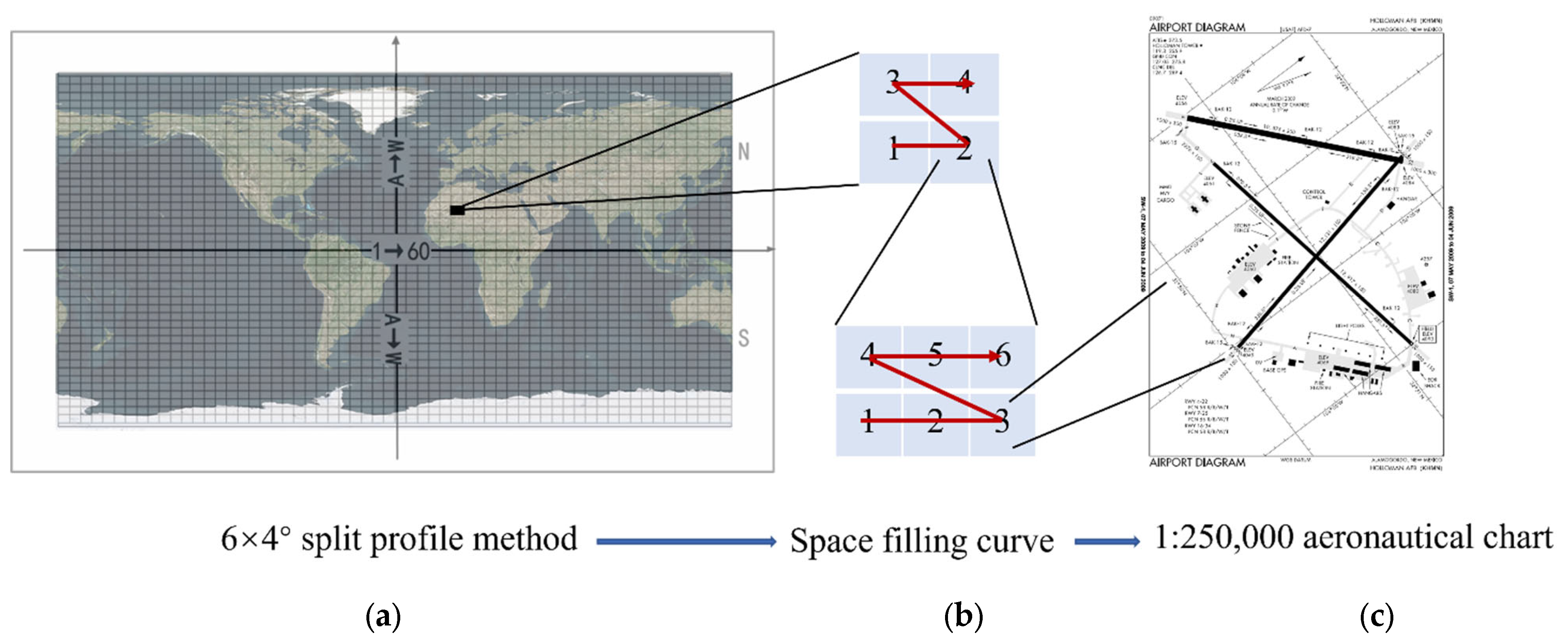
The size of the first dissected grid cell is 6° × 4°. The Northern and Southern Hemisphere identification codes are N and S, respectively; whereas the longitude direction is coded with 01–60, whereas the latitude direction is coded from the equator to the northern and southern hemispheres according to A–W. The coding direction is shown in Figure 2a. This profiling method corresponds to 1:1,000,000 charts, whereas the second profiling is in the form of 3° × 2°, and the space is coded as 1–4 according to the z-order (1:250,000 charts, as shown in Figure 2b). The degree level profile is in the form of 1° × 1°, corresponding to a 1:50,000 charts, and the above-degree level profile is regarded as the primary profile method of the airspace grid GeoSOT-AS.

(b)

Coding method for secondary profile blocks.

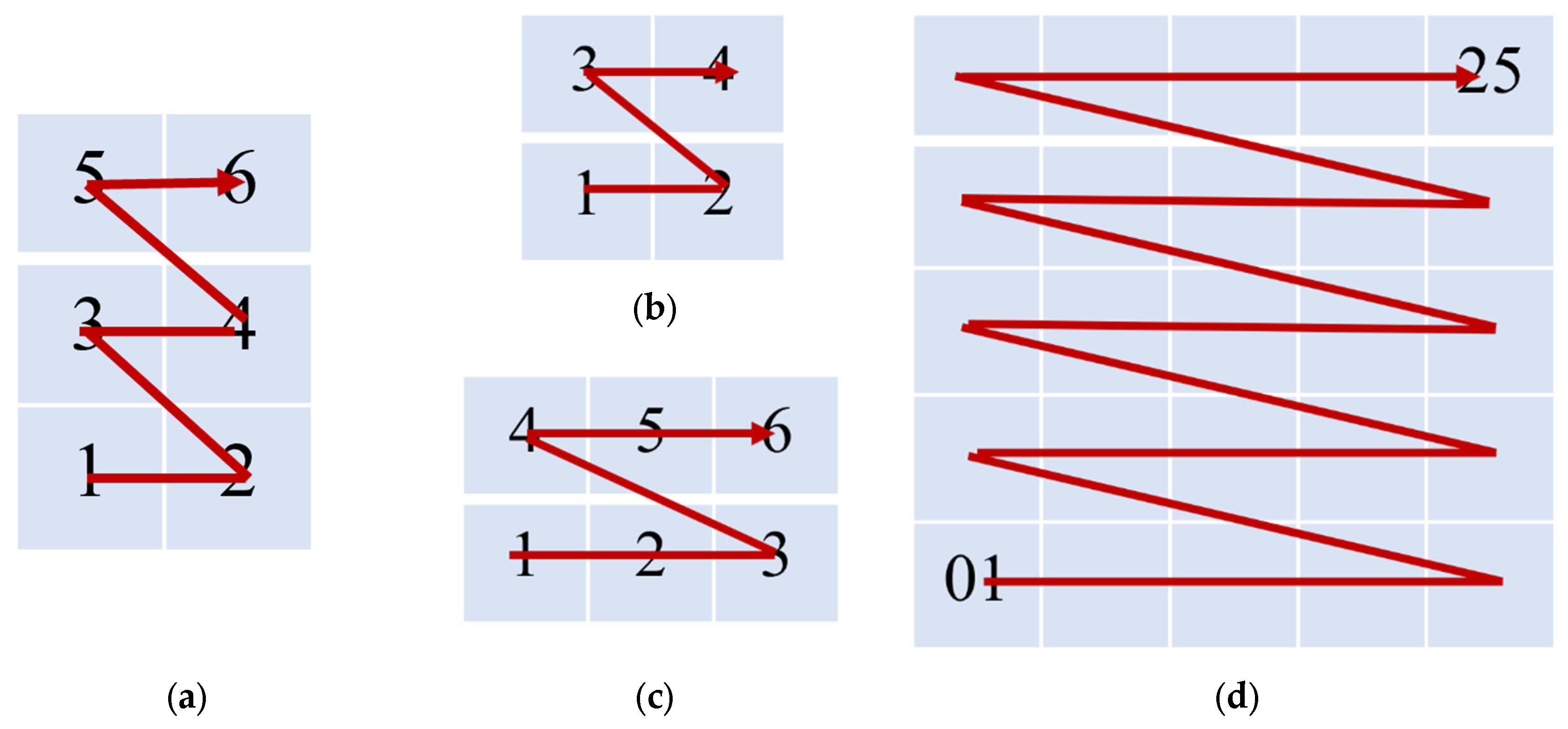
There are seven levels of secondary blocks, corresponding to four types of profiles, 2 × 2, 2 × 3, 3 × 2, and 5 × 5 of the previous grid, coded in z-order as 1–4, 1–6, 1–6, and 01–25 respectively, with the finest profile granularity set to the second level. Here we need to emphasize that in the 6th to 7th and 10th to 11th levels of segmentation, there is a two-digit representation, whereas in the other levels, only one digit is required.

The size of each level of the grid scale and its coding bit representation for the above GeoSOT-AS profiling method, as well as its corresponding coding method are shown in Figure 4.

Figure 5 shows the coding bits and their representation from the 1st to 11th levels, where each digit is denoted by an asterisk *. Based on the above profiling and given coding methods, an example specified planar airspace area with a profiling range of [108°30′29″, 108°30′30″], [23°35′25″, 23°35′26″] can be progressively derived according to the completion of level-by-level profiling, and the principle of coding bit matching. In this example, the area code is N49F344140114206, where each digit or combination of digits corresponds to the dissection scale, and the prefix interception can be performed according to the requirements of different levels to determine the dimensional range of the previous level’s plane.

3.2. GeoSOT-AS Height Dimensional Profiling Rules and Methods

3.2.1. Height Dimensional Profiling Rules

Oriented to the management of airspace and its elements, it was proposed to adopt the principle of flight altitude layers for profile selection across the height dimension. Regarding the flight altitude, the following base definitions were applied:

The corrected sea level pressure height (QNH) refers to the pressure height with the corrected sea level pressure as the datum.

Standard barometric height (QNE) refers to that with the standard sea level pressure as the datum.

The flight altitude layer was divided by a certain altitude difference, with the standard atmospheric level serving as the reference plane. Equipping aircraft on different altitude layers, so that there is a specified safety altitude difference between aircraft, is an important measure to prevent aircraft collisions with each other or ground obstacles.

In the flight path, if the QNH is used as the altimeter correction value, the aircraft will frequently adjust the QNH after passing through different areas, and it remains difficult to determine the vertical separation between aircraft. Therefore, using QNE as the altimeter correction value can simplify the flight operation, and ensure the altitude safety interval between aircraft.

Based on the QNE altitude dialing positive values, the basic definition of flight altitude layers, and the division criteria, the following principles of altitude stratification coding were set corresponding to the segmented step function, yielding the following expressions (Equation (2)):

$$Code\left(h\right)=\left\{\begin{array}{l} Cod{e}_2 Fleve{l}_2\le h<Fleve{l}_3 \\ Cod{e}_1 Fleve{l}_1\le h<Fleve{l}_2 \\ Cod{e}_0 Fleve{l}_0\le h<Fleve{l}_1 \\ \hfill \dots \dots \hfill \end{array}\right.$$

(2)

Considering that the required flight airspace ranges from 0 to 50,000 m, one must consider the existence of areas on the surface with elevations <0 m (e.g., the Turpan Basin in China lies at −154.31 m). To ensure the uniformity and multi-scale of the division, while considering the general civil aviation use airspace ≤50,000 m, the coding support range was set from −150 to 76,800 m, and the specific division rules were as follows. Firstly, the overall range divided into two parts: −150 to 0 m, and 0 to 76,800 m, with 0 identifying the area above sea level, and 1 indicating the area below sea level (i.e., the first unsigned integer is used to mark the above or belowground); secondly, combined with the actual Chinese flight altitude layer division standards, the current flight altitude layer was divided into 10 levels via bifurcation, with the finest granularity in the discrete form of 150 m. The corresponding altitude layer interval for each level is shown in

Table 2. Recursive scales for height dimensional profiling.

Level	Height Interval (m)	Level	Height Interval (m)
1	76,800	6	2400
2	38,400	7	1200
3	19,200	8	600
4	9600	9	300
5	4800	10	150

.

3.2.2. Height Dimensional Coding Methods

Under the operation of level-by-level dissection across the height dimension, the right and left tree characters were assigned values of 1 and 0, respectively, for each binary tree, in order to dissect to the lowest level, and achieve the requirement of 150 m hierarchy. The specific dissection and coding schematic is shown in Figure 6.

In general, a distinct height code can be utilized to indicate the range of height layers, as per typical civil aviation guidelines for ADS-B data analysis which specify a separation of 300 m between height layers. For instance, if an aircraft is flying at an altitude of 8400 m, the altitude layer multi-level profile principle mentioned above represents its operation using the code 0 00010001 for high-level airspace.

3.3. GeoSOT-AS Time Dimensional Profiling Rules and Methods

GeoSOT-T dissection theory [42] describes the segment-by-segment dichotomy and multiscale encoding of time, and relies on encoding clustering for fast retrieval of data containing temporal information. This info primarily takes the forms of the expansion of 1 y into 16 mo, 1 mo into 32 d, 1 d into 32 h, 1 h into 64 min, 1 min into 64 s, 1 s into 1024 millisec, and 1 millisec into 1024 microsec in a limited time domain (65536 B.C.–65535 A.D.) by co-primary temporal binary expansion. Through these expansions, the binary tree structure of year, month, day, hour, minute, and second is thus realized, forming a 64-level binary tree with time scales as large as 130,000 years after B.C. (level 0), and as small as microsecond (level 63). The time slice binary tree constitutes a multi-scale, uniform discrete-time coding system.

Based on the flow form of ADS-B data, it was proposed to use three expansions, whereas for the data cycle by day, it was proposed to use the extraction of partial layers for coding representation, three expansions way time expansion (

Table 3. Time division scheme.

	Hour	Minute	Second
Original range	0–24	0–60	0–60
Extended range	0–32	0–64	0–64

), in order to fit the binary integer profile (i.e., 0–24 h daily time span was expanded to 0–32 h, 0–60 min was expanded to 0–64 min, 0–60 sec was expanded to 0–64 s. For example, first set the time range, based on the form of ATC data, for example, set to [2020-04-26 00:00:00, 2020-04-26 24:00:00), that is, based on the form of data flow of a day to do the analysis. To describe the entire day span, three different expansions are utilized. These expansions employ the bifurcation dissection principle of GeoSOT-T, using the Table 3 expansion format to achieve the goal of integer bifurcation dissection.

The time code format is shown in detail below:

$$\underset{\mathrm{unsigned}}{\underbrace{0}} \underset{\mathrm{hour}}{\underbrace{10010}} \underset{\mathrm{minute}}{\underbrace{100101}} \underset{\sec \mathrm{ond}}{\underbrace{110011}}$$

where the advantage of integer bifurcation is that the data of the same time period can be given the same prefix, whereas the data requests within a time period can be based on the prefix index of the database, instead of retrieving the timestamp information of the whole cross-domain in turn. This process ultimately simplifies the time period query in database retrieval to a simple binary-coded matching query, which greatly reduces the retrieval cycle.

4. GeoSOT-AS-Based Gridding Modeling Method for Airspace Information

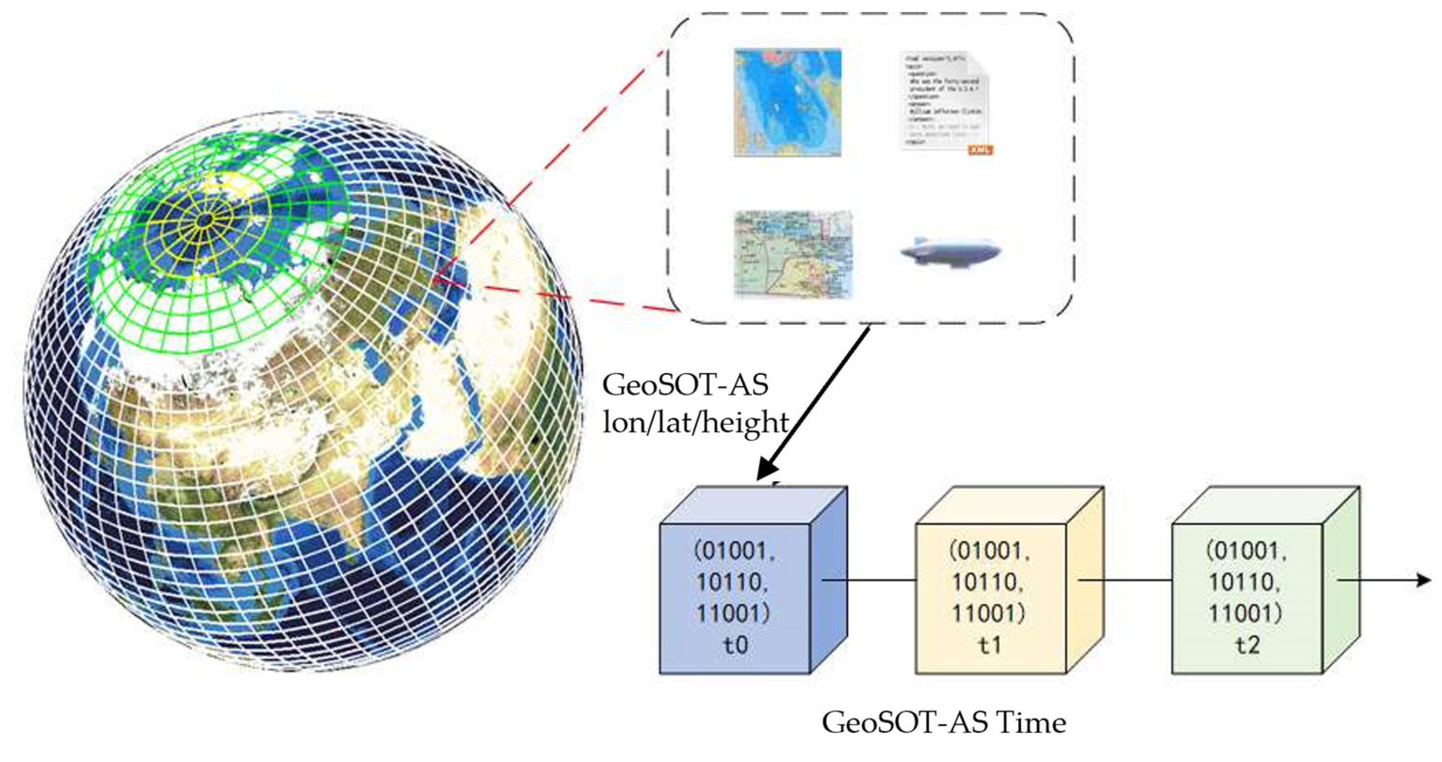
The management of each element of ATC information is actually the mapping and representation of ATC data information (etc.) across the entire airspace, represented by ADS-B. Each ATC element with spatiotemporal information can be modeled and designed under the GeoSOT-AS model framework, i.e., the moments and their locations corresponding to each information point can be abstracted as attribute information under the GeoSOT-AS framework. The ADS-B data under GeoSOT-AS model not only has its own spatial location attributes, but contains other spatial extension attributes as well, such as its accompanying flight number and landing and takeoff airports. Compared with the 3D raster data model, where the spatial location is identified by the local coordinates of the raster, in the GeoSOT-AS model, the spatio-temporal location attributes can be identified by the coding of the unified transformation of latitude, longitude, height, time, etc. The specific architecture is shown in Figure 7.

The logical modeling of ADS-B information records the code of the profile element at its spatial location, as well as the entity properties, and the 3D profile modeling of the point can be expressed by Equation (3):

$$\left\{\begin{array}{l}{P}_{AS-subdivision}=COD{E}_n\stackrel{g}{\leftrightarrow }SU\\ COD{E}_n=f\left(L,B,H,T\right)\\ A_p=A_{su}\end{array}\right.$$

(3)

where (L, B, H, T) are the longitude, latitude, altitude, time and other element information of the location in the airspace space, respectively, and the corresponding value is determined by that of it profile level, where SU is the profile element of the track point-like entity under the corresponding profile level, and CODE_n is the profile code of the track point data under this level, indicating that the attribute data of the track point is inherited by the attribute of the profile element at this time. For the ADS-B data with latitude, longitude, elevation and time information, the proposed conversion algorithm of airspace grid (GeoSOT-AS) encoding is used for processing, and the specific calculation steps include: encoding of latitude and longitude information with airspace grid, encoding conversion of altitude information, and conversion encoding of time information.

4.1. Longitude and Latitude Information Conversion Coding Algorithm

After extracting the latitude and longitude information of the airspace target, the corner point coordinates of the airspace target location are calculated stepwise according to the selected planar dimensional profile range level according to the profiling method in Section 3.1, and the iterative operation was performed according to the rounding and remainder, with the assignment rules carried out according to the filling curve, and the specific algorithm flow is shown by Algorithm 1:

Algorithm 1 Grid set generation algorithm for latitude and longitude

Input: Location information for ADS-B data point source ($Lng,Lat$), level $L$ Output: ADS-B data plane dimensional grid coding set 1.  function EncodeLocation($Lng,Lat,L)$ 2.  if $L==1$ then 3.  Step1: Obtain hemisphere identifiers in which ($Lng,Lat$) is located 4.  Step2: Calculate the latitude and longitude direction identification code 5.  Step3: Get the first level grid for the location 6.  elif $L > 1$ then 7.  $for i in range\left(1,L\right):$ 8.  Calculate 9.  $a_i=\left[\left(Lng-{\lambda }_{i-1}\right)/({\Delta }_L\lambda \right]+1$ 10. $b_i=\left[\left(Lat-{\varphi }_{i-1}\right)/({\Delta }_L\varphi \right]+1$ 11. $Lng\leftarrow Lng-{\lambda }_{i-1}$ 12. $Lat\leftarrow Lat-{\varphi }_{i-1}$ 13. ${\lambda }_i, a_i$ the longitude of the position angle point and column number 14. ${\varphi }_i, b_i$ the latitude of the position angle point and row number 15. $p_i={\alpha }_i{a}_i+{\beta }_i{b}_i$ ${\alpha }_L,{\beta }_L$ is determined by the current fill curve 16. $P_{code}=p_1{p}_2\dots p_L$ 17. End if 18. $return P_{code}$ 19. End function

4.2. Height Information Encoding Conversion Algorithm

The height dimension information coding conversion algorithm was based on the aforementioned altitude dimension dissection method presented in Section 3.2, which can obtain the coding of the highest level based on the underlying structure of the 150 m segmented flight altitude layer and obtain the coding representation of the lower level by intercepting the prefix based on the clustering of the coding prefix. The specific algorithm flow is shown by Algorithm 2:

Algorithm 2 Grid set generation algorithm for height

Input: Height information for ADS-B data point source ($Height$), level $L$ Output: ADS-B data height dimensional grid coding set 1.  function EncodeHeight($Height,L)$ 2.  $h_0=1 if Height>0 else h_0=0$ 3.  ${\left\{\Delta H\right\}}_{i=1}^L=150m*2^{11/i}$ 4.  $for i in range\left(L\right):$ 5.  $if Height<\Delta H_i:$ 6.  $h_i\leftarrow 0$ 7.  else: 8.  $h_i\leftarrow 1,Height=height-\Delta H_i$ 9.  $H_{code}=h_0{h}_1{h}_2\dots h_L$ 10. End if 11. End for 12. $return H_{code}$ 13. End function

4.3. Time Information Coding Conversion Algorithm

The temporal information encoding conversion algorithm is based on the temporal dimensional profile and its encoding method in the aforementioned Section 3.3. Based on three time extensions, the highest level of time encoding is obtained with the lowest interval second level unit as the criterion, and subsequent interception calculations can be performed based on different time intervals and level criteria (Algorithm 3):

Algorithm 3 Grid set generation algorithm for timestamp

Input: Time information for ADS-B data point source ($Time$), level $L$ Output: ADS-B data time dimensional grid coding set 1.  function EncodeTime($Time,L)$ 2.  $t_0=0$ 3.  ${\left\{\Delta T\right\}}_{i=1}^L=1s*2^{17/i}$ 4.  $for i in range\left(L\right):$ 5.  $if Time<\Delta T_i:$ 6.  $t_i\leftarrow 0$ 7.  else: 8.  $t_i\leftarrow 1,Time=Time-\Delta T_i$ 9.  $T_{code}=t_0{t}_1{t}_2\dots t_L$ 10. End if 11. End for 12. $return T_{code}$ 13. End function

5. GeoSOT-AS Based Regional and Time Segment ADS-B Data Extraction Algorithm

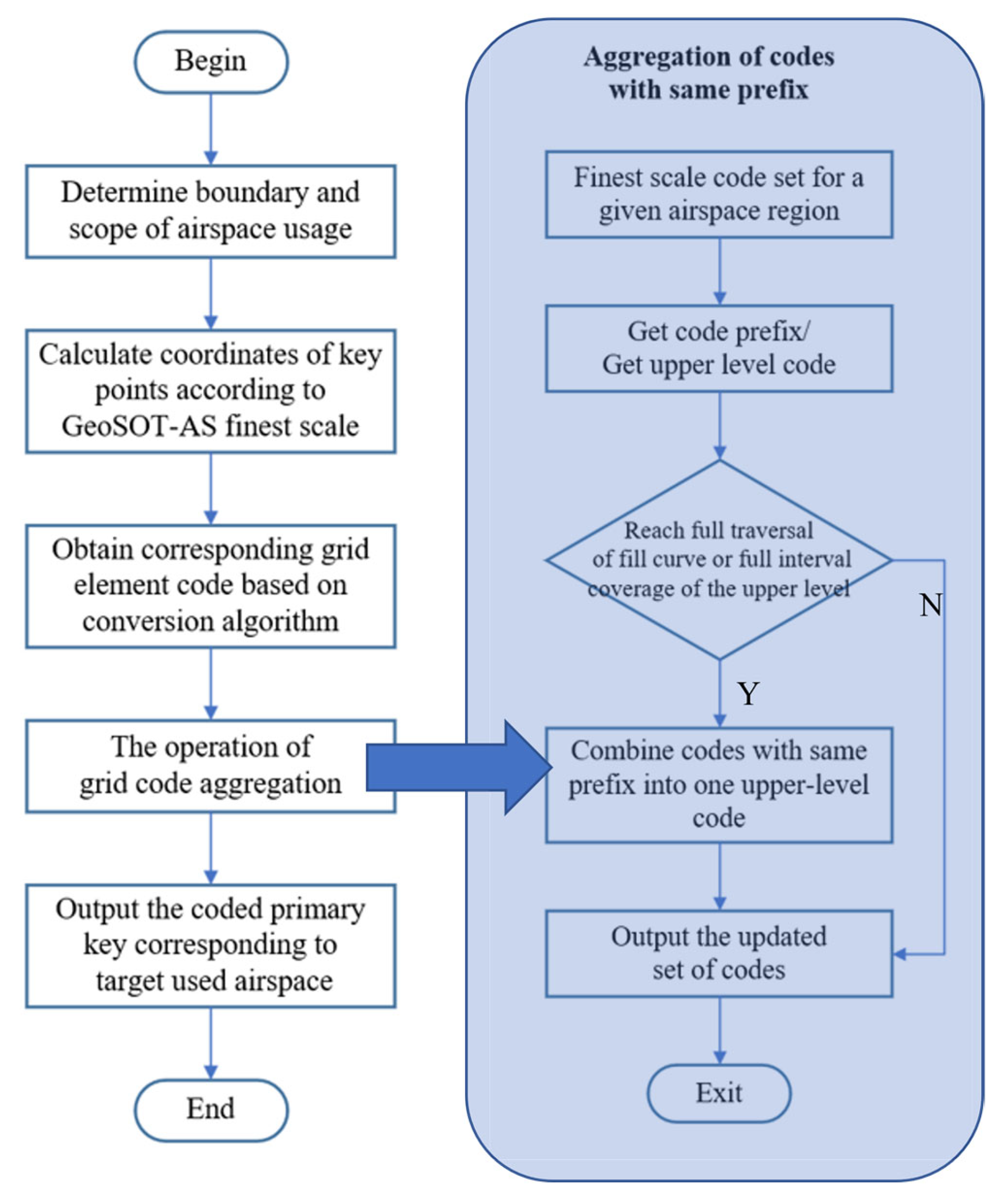
The search includes ADS-B and its corresponding attribute data, including flight speed, heading, aircraft type, and so on. ADS-B data extraction is a search for the required data from the aerial database, which in essence is a query for data and attributes of spatial entities according to certain conditions, forming a new subset of spatial data, organizing the data according to the spatial location, and directly extracting multiple attributes corresponding to the spatial location through the grid code. In this process, it is necessary to convert the retrieved spatial range into a set of segmentation elements covering the query area and use the set of codes to directly query the attribute information with the spatiotemporal matching of ADS-B data.

The method actually converts the latitude and longitude heights as well as the temporal cross-domain range into a primary key query that is coded instead. Due to the multi-layer profile structure, the index can be defined as the finest level first, and then the index aggregation can be performed using the prefix matching property of the code. The flow chart is shown as Figure 8.

5.1. Finest Granularity Matching

This step of the operation consists in matching the finest granularity of the profile scale with the span range of latitude and longitude heights, as well as time to output the location of the finest level of coding retrieval, as described in Section 3. Determining the longitude values for extracting the maximum and minimum longitude surfaces of the spatio-temporal representation area, denoted as $Di{s}_L=L_{max}-L_{min}$, the latitude of the maximum and minimum latitude surfaces of the spatiotemporal representation area, denoted as $Di{s}_B=B_{max}-B_{min}$, the maximum and minimum values of the elevation of the spatiotemporal representation area, denoted as $Di{s}_H=H_{max}-H_{min}$, and the span of the time range of the spatiotemporal representation area, denoted as $Di{s}_T=T_{max}-T_{min}$.

The latitude and longitude heights, as well as the temporal finest granularity are described in Section 3, and setting them to $\Delta p,\Delta h,\Delta t$ constants give the coordinates of the key finest granularity corner points by a similar interpolation method (Equation (4)):

$$\begin{gathered} x_i=L_{min}+Di{s}_L/\Delta p \\ {y}_i=B_{min}+Di{s}_B/\Delta p \\ {h}_i=H_{min}+Di{s}_H/\Delta h \\ {t}_i=T_{min}+Di{s}_T/\Delta t \end{gathered}$$

(4)

where the most fine-grained matching process T is defined as follows: for the region corner point information $P\left(x_i,y_i,h_i,t_i\right)$, where if $P\left(x_i,y_i,h_i,t_i\right)$ is within the cell of grid dissection $Cel{l}_i$, i.e., there is $P\left(x_i,y_i,h_i,t_i\right)\in Cel{l}_i$, then it is indicated that $Cel{l}_i$ represents the retrieval area of range span $\left(x_i,x_i+\Delta p\right),\left(y_i,y_i+\Delta p\right),\left(h_i,h_i+\Delta h\right),\mathrm{and}\left(t_i,t_i+\Delta t\right)$ (Equations (5) and (6)):

$$T\left(P\left(x,y,h,t\right)\right)=\left\{\begin{array}{l}Cel{l}_i,P\left(x,y,h,t\right)\in Cel{l}_i\\ 0,P\left(x,y,h,t\right)\notin Cel{l}_i\end{array}\right.$$

(5)

Under this condition, the specific code form $Cod{e}_i$ of $Cel{l}_i$ can be obtained according to the code conversion method in Section 4, which results in the mapping relationship f between the fine-grained grid set, and the retrieval range span.

(6)

5.2. Grid Code Aggregation

When the finest granularity of grid voxels was set to match the retrieval range, in general, the number of retrieval codes increased as the retrieval range expanded. Here, to avoid the retrieval of excessive finest granularity grid codes, a regional aggregation method was proposed based on grid voxel codes, which uses the prefix consistency of codes for code aggregation to reduce the number of index codes.

The coding bit operation is introduced, and simply, the prefix extraction function of codes $Cal\_Sub\left(Cod{e}_v,i\right)$ is proposed. To obtain the prefix code before the $i$th bit of the encoded interval (Equation (7)):

$$Cal\_Sub\left(Cod{e}_v,i\right)==Code>>\left(Cod{e}_{len}-i\right)$$

(7)

where the idea of encoding interval extraction is to truncate the encoding by shifting $\left(Cod{e}_{len}-i\right)$ bits to the right to clear the high bits on the right side, whereas obtaining the first $i$ bits of the encoding $Cod{e}_v$, where $Cod{e}_{len}$ is the original fine-grained encoding bits.

In general, for the set of mapping codes in the first step, it is only necessary to consider the case of consistent prefix codes in the appropriate code bits to reach the full traversal of filling curves, or full interval coverage of the upper level. Then one can perform simple upward aggregation, via multiple codes with the same code prefix which can be aggregated into one upper-level code. Under these conditions, not only to ensure the consistency of the index range, while avoiding unnecessary code index redundancy, the code aggregation process formula was expressed as follows: $Cod{e}_{ini}$ is the encoding prefix for the upcoming aggregation operation (Equations (8) and (9)):

$$Cell\_Merge={\displaystyle \sum }_{i=0}^n{\partial }_i*Code\left(i\right)$$

(8)

$${\partial }_i\left(Cod{e}_v\left(i\right)\right)=\left\{\begin{array}{c}0,Cal\_Sub\left(Cod{e}_v,i\right)\ne Cod{e}_{ini}\\ 1,Cal\_Sub\left(Cod{e}_v,i\right)=Cod{e}_{ini}\end{array}\right.,i=0,1,\cdots ,n$$

(9)

6. Experiments and Results

This section describes the specific experimental design as well as the experimental data to design three parts of experiments.

One is the GeoSOT-AS shape variation law analysis experiment, which corresponds to the content of the airspace spatiotemporal grid framework to demonstrate its usability for ADS-B data carrying under shape variation, whereas the other is the ADS-B data space-time grid modeling experiment to demonstrate the low cost of encoding calculation and data modeling in the airspace spatiotemporal grid framework. The last two experimental designs verified the high performance of extracting ATC region data in the GeoSOT-AS, i.e., to verify that the speed of extracting target airspace information data with GeoSOT-AS coding as the main key functioning better than the general data extraction methods based on latitude, longitude, and MongoDB’s own spherical index, so as to respond to the need of extracting immediate ATC data for large-scale air use and planning, and as the basic guarantee of airspace digitalization and information management. It is a basic guarantee for the digitalization and information management of airspace.

6.1. Experimental Environment

The specific hardware and software environment is described as follows:

The selected MongoDB database is deployed in single node mode on a physical server with base development languages, such as database language, python and Javascript. The server runs a CPU (3.6GHz Intel Core i7 CPU), 16GB of RAM and a 1TB hard drive. The server is running on Windows 10 pro 64-bit operating system. The following experiments and designs are based on the hardware and software environments described in

Table 4. Software and hardware environment.

Hardware		Software
Processor	Inter(R) Core i7-7700 @ 3.60 GHz	OS	Windows 10 pro (64×)
Memory	16 GB	Tools	Python, JavaScript
Storage	1 TB	Database	MongoDB

.

6.2. Experimental Data

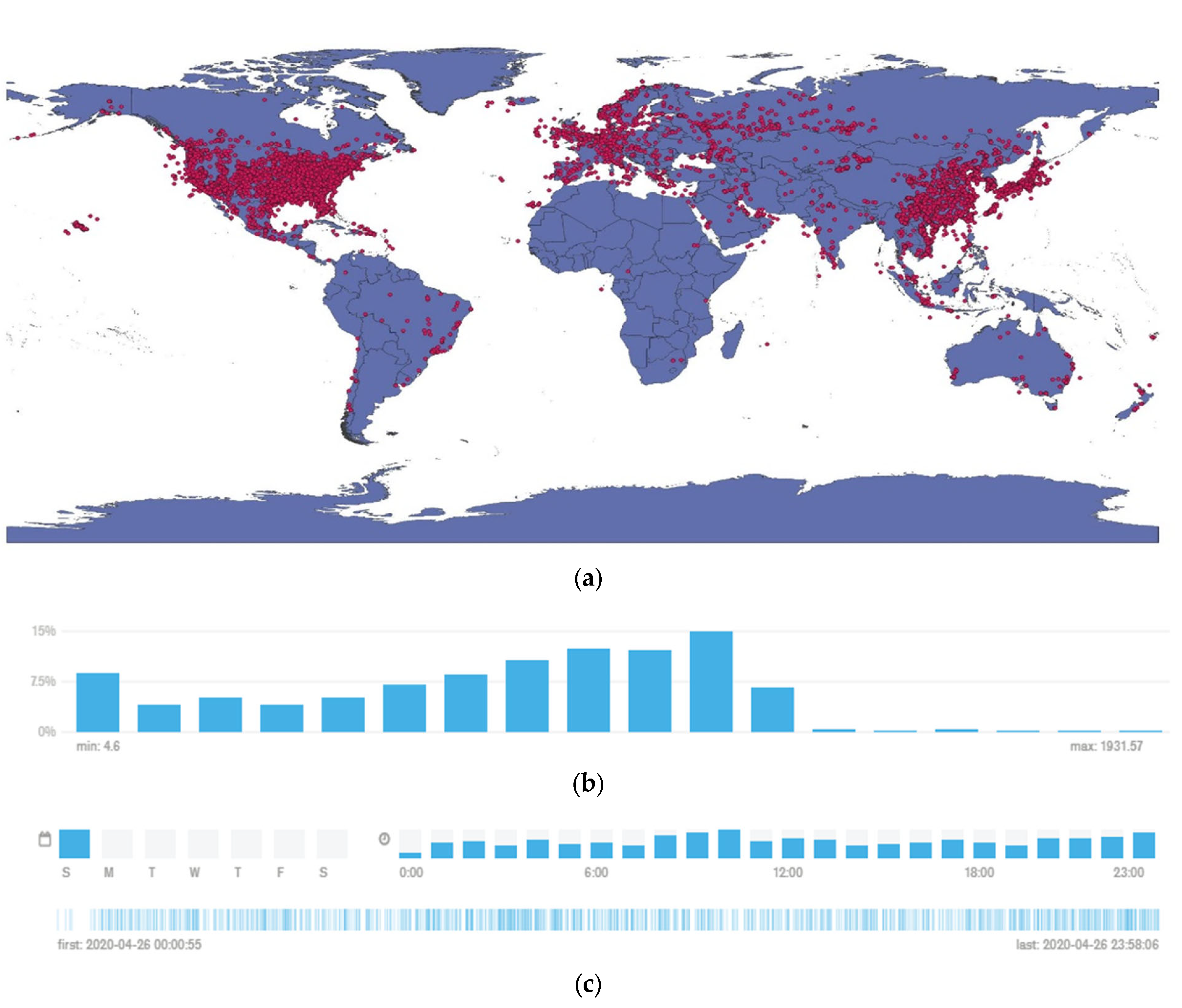
The data used in this experiment are global one-day ADS-B data, and the Opensky ADS-B interface in the traffic toolbox [43] to supplement the received data with a total of ~16 million ADS-B data.

Specific flight parameters include flight identification information (flight number or call sign), ICAO 24-digit aircraft address (globally unique airframe code), real-time position (latitude and longitude), position integrity and accuracy (GPS horizontal interval limit), barometric and geometric altitude, vertical change rate (climb/descent rate), track angle and ground speed, and emergency indication; specialized position identification information, etc., are shown in

Table 5. ADS-B data structure and its example description.

Data Attribute	Type	Example
Track ID	Integer	3
Flight number	String	CCA4392
Secondary code	String	CA
Departure airport	String	ZGSD
Landing airport	String	ZUUU
Model	String	A320
Longitude	Integer	104.373
Latitude	Integer	29.7987
Height (10 m)	Integer	359.7
Direction	Integer	315
Speed (km·h−1)	Integer	680
Time	ISODate	2020-04-26T00:00:00Z

.

A data distribution overview chart (Figure 9) was formed by randomly sampling data points to study their composition. The chart shows that the information points are primarily concentrated in three regions of East Asia, Central America and Europe. The majority of information points in the airspace are located at altitudes of ≤12,000 m, with only a few outlier information points falling in the 12,000–20,000 m range. Note that the time distribution is more uniform, and that information regarding all times is expressed.

6.3. GeoSOT-AS Shape Change Law Analysis Test

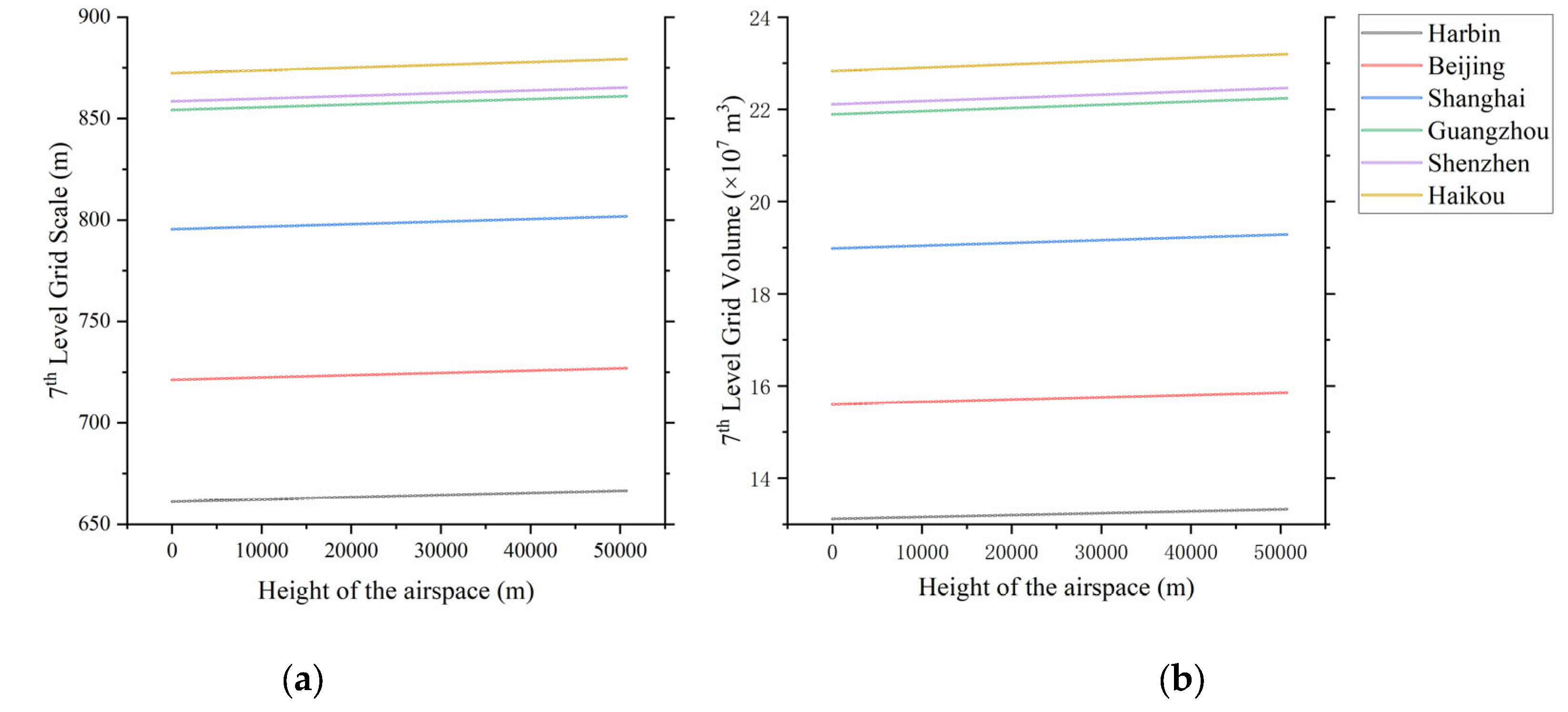
This section demonstrates the availability and consistency within a certain error of the Chinese domestic airspace and similar airspace regions under this segmentation framework; thus, it serves as one of the criteria for the rationality of the ADS-B data carrying framework. In this section, the 300 m stratification and the planar dimensional profile of the grid at the eighth level (~1 km level) were selected for two aspects of index analysis, and the airspace at typical representative locations in China, including the following six regions: the extreme locations of the north and south latitudes, and the airspace in the north, south, wide and deep areas where the airspace traffic and utilization rates in China are relatively dense, and the deformation law of the grid edge length and grid capacity, or the deformation law of the grid volume is calculated. The shape variation of the regional grid was analyzed.

The variation pattern of grid edge length and grid volume for each location is shown below. Figure 10a shows the variation pattern of grid edge length with height layer, and Figure 10b shows the variation pattern of grid volume with height layer.

From Figure 10, it was observed that the grid deformation in the same area varies less with altitude (i.e., in the spatial range of airspace <50,000 m, the local airport and urban airspace grid can be approximated to a uniform scale size, which is suitable for unified airspace planning and zonal block management of ADS-B data with a local deformation rate of 0.8%). Alternatively, for longitudinal observation, the grid deformation ratio equation was set for different regions of China. The grid scale of the airspace at marker $i$ was set to ${\mu }_i$, the standard ratio parameter calculation selects the grid scale of GeoSOT-AS standard level 7, set to ${\mu }_{norm}$; whereas the maximum deformation rate equation is expressed by Equation (10):

$$S_{deflection}=\left|\frac{{\mu }_i-{\mu }_{norm}}{{\mu }_i+{\mu }_{norm}}\right|.$$

(10)

Similarly, the deformation rate of the grid volume was expressed by Equation (11), the grid scale of the airspace at mark j is set to ${\sigma }_j$, and the standard volume under the 300 m height layer is set to ${\sigma }_{norm}$, which is the standard block volume calculated by the grid scale of the seventh level of GeoSOT-AS standard, and the deformation rate of the grid volume is expressed by Equation (11):

$$V_{offset}=\left|\frac{{\sigma }_j-{\sigma }_{norm}}{{\sigma }_j+{\sigma }_{norm}}\right|.$$

(11)

From the above formula, the base deformation rate analysis table was drawn (

Table 6. Maximum deformation rate analysis.

Location	Grid Scale (km)	Max Deflection Rate	Volume ( $\times$107 m3)	Volume Change Rate
Harbin	0.667	0.164	13.347	0.319
Beijing	0.727	0.121	15.856	0.239
Shanghai	0.802	0.073	19.296	0.145
Guangzhou	0.861	0.037	22.239	0.075
Shenzhen	0.865	0.035	22.447	0.070
Haikou	0.879	0.027	23.180	0.054

).

As can be seen from the above table, in the airspace of important locations in China, and at the same latitudes, the maximum GeoSOT-AS grid edge length scale is at around 16% deformation, whereas the maximum grid volume offset rate is 31.9%, within a certain management error range. There is no obvious conflict between this degree of deformation rate and volume offset rate, and the actual use under the framework of the four-dimensional spatiotemporal grid of this airspace for the actual ADS-B data. The organization method and extraction of the actual corresponding air charts were reasonable, complete, and in line with the actual ADS-B data storage and use requirements.

6.4. ADS-B Data Spatiotemporal Gridding Modeling Experiments

After establishing the data representation relationship of airspace grid spatio-temporal information, a MongoDB-based grid database was created for airspace management, using the grid spatiotemporal code as the primary key of the database to make full use of the query, and retrieval of the string code. The table structure is designed as follows: each subdivision element maps a subdivision element code and multiple aircraft objects (there can be multiple aircrafts in a grid at the same time); thus, they can be organized by grid data and aircraft object data. The multiscale grid aviation database is created using the multiscale prefix feature of the grid. The ADS-B data design for the database table structure is shown in

Table 7. ADS-B information structure table under GeoSOT-AS framework.

Database (Table) Structure	Note
{
“GeoSOT-AS Code”:[ PCode: N49F461611434217 Hcode: 1 1011010 Tcode: 0 10010 100101 110011 ],	Planar code Height code Time code
“data_exisit”:1,	Data source identifier
“dataid”:603e3a3fb9a39c8dbd9245e8
“data”:[
Attribute_I:{	information (I) property class
“B”:104.373	Longitude
“L”:29.7987	Latitude
“H”:359.7	QNE
“Direction”:315
“T”: 2020-04-26T00:00:00Z	ISODate
“v”:680	Speed
}
Attribute_S:{	situation(S) property class
“Fnum”:CCA4392	Flight number
“Type”:A320
“DA”:ZGSD	Departure airport
“AA”:ZUUU	Arrival airport
}] …
}

.

The results of the coding conversion time for different data volumes—20%, 40%, 60%, 80%, 100%—are shown in

Table 8. Coding conversion time results.

Data Amount	20%	40%	60%	80%	100%
Conversion time (ms)	0.02	0.13	1.15	12.91	109.89

.

It is observed that ADS-B data conversion for the entire day, using the coding conversion method outlined in Section 4, takes only a hundred milliseconds for conversion on the order of ten million data points, at various ratios of the complete data volume, and the cost of coding conversion is less. Thus, the coding conversion time advantage is more obvious when the data volume is lower due to the machine performance, and it is clear from the above analyses that the method is less time costly and more operable.

6.5. Fixed-Time Temporal Range Indexing

A randomly selected time period of interest “2020-04-26 00:00:00”–“2020-04-26 24:00:00” was selected for the whole day, and

Table 9. Geographical information of the test area.

Lower Left Corner Coordinates	Upper Right Corner Coordinates	Height Range
(118.193828° E, 24.492242° N)	(119.19387° E, 24.702114° N)	0.0–9.6 km
(11.849844° E, 44.002925° N)	(11.997022° E, 44.109069° N)	3.6–8.1 km
(63.655784° W, 37.168087° N)	(62.772714° W, 37.988062° N)	4.8–10 km
(111.195247° E, 33.305296° N)	(112.078317° E, 35.500992° N)	8.1–12 km
(144.899094° E, 21.299828° S)	(145.634986° E, 27.889033° S)	3.0–6.0 km

displays the specific information regarding the spatial extent of interest. Each set of data in the table forms a cube that encloses a box. The objective is to test the average efficiency of spatiotemporal filtering queries.

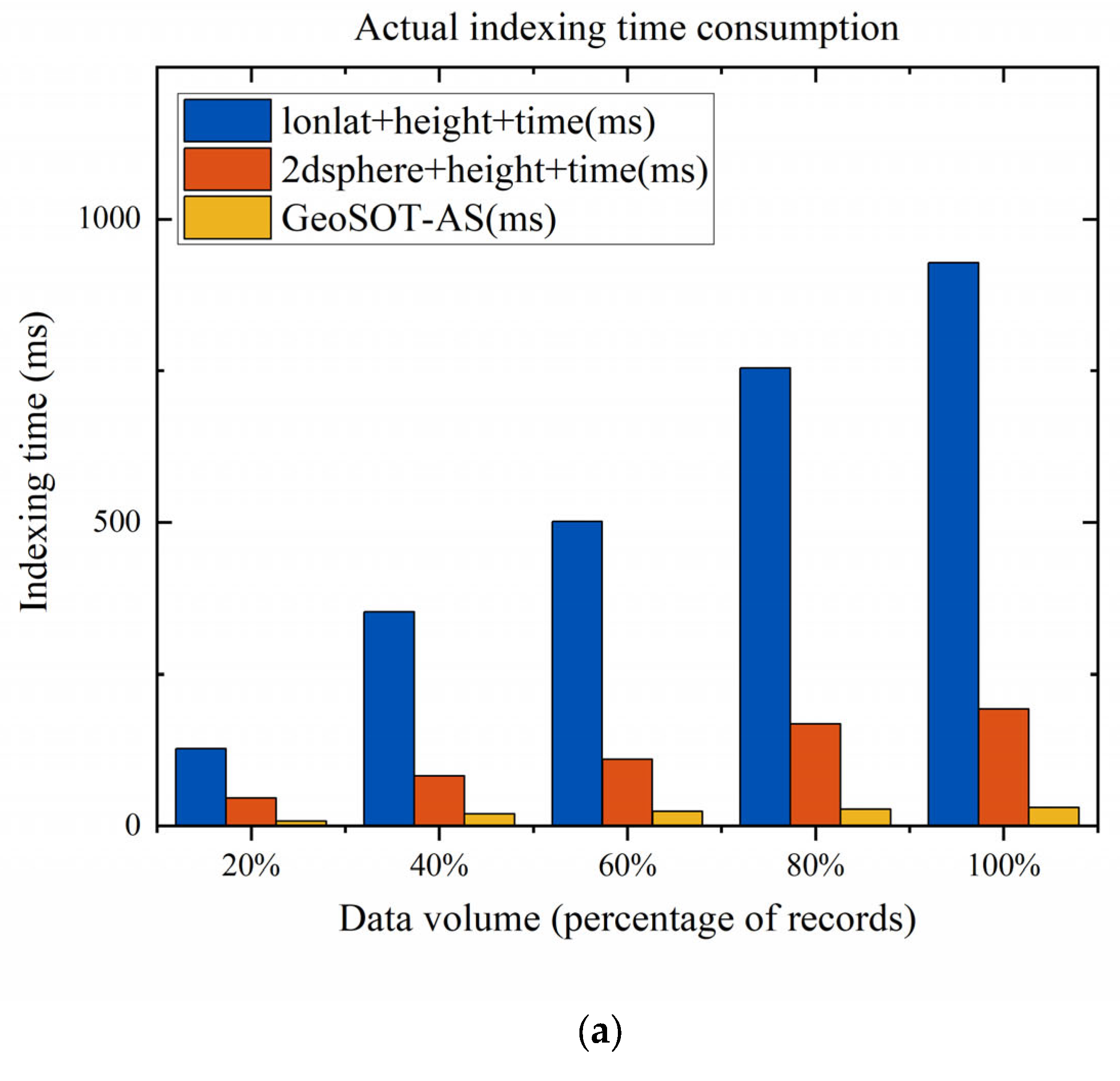
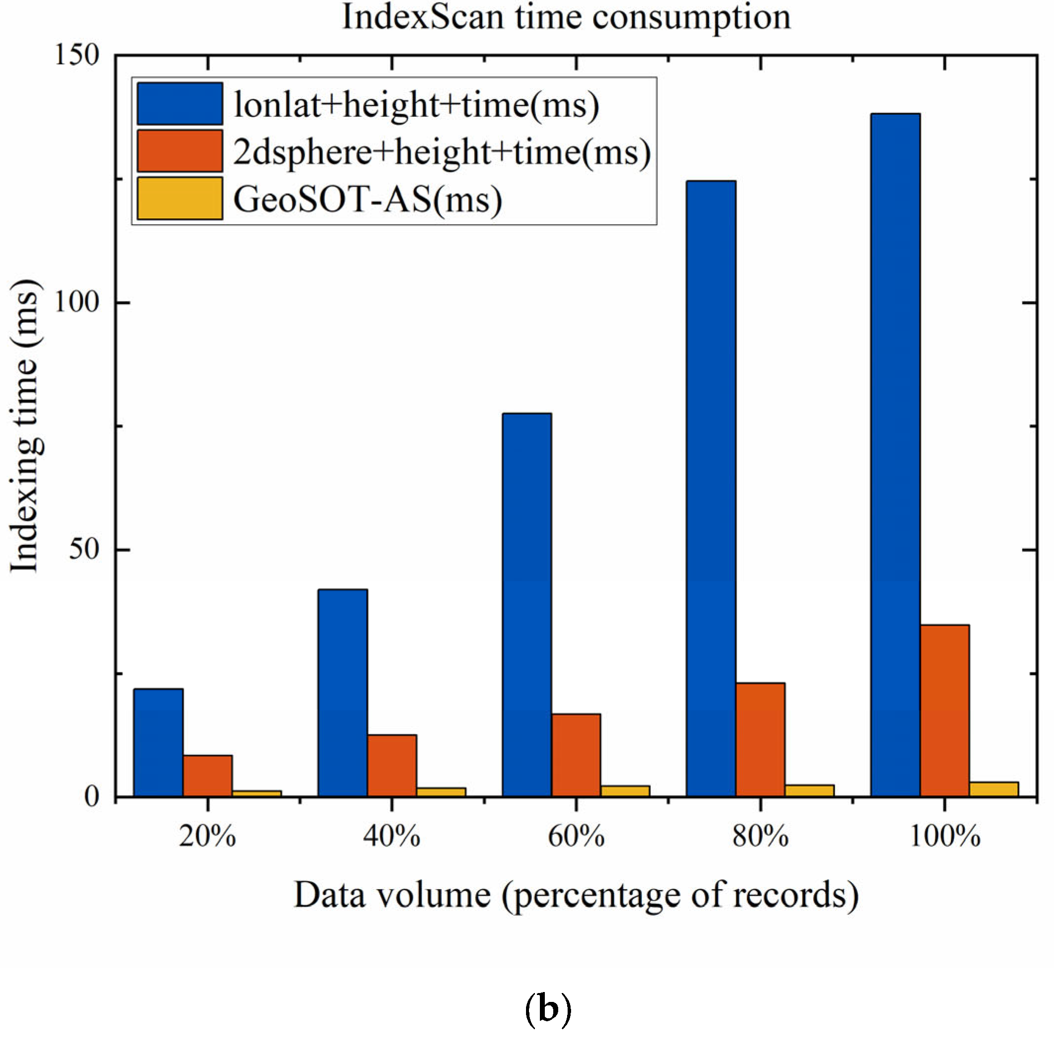
According to different data volume—20%, 40%, 60%, 80%, and 100%—the efficiency of spatiotemporal indexes constructed in three ways was tested. First, MongoDB’s own spatial index based on latitude and longitude was used, plus time dimension and data id to construct a composite spatiotemporal index. Second was MongoDB’s 2dsphere spatial index, plus time dimension and data id to build composite spatiotemporal index. The third way was the use of a spatiotemporal index based on space-time grid encoding as index primary key. The three methods are named as LLHT index, 2dsHT index, and GeoSOT-AS code index, accordingly. Take the first row of data as an example to introduce the three different forms of indexing, which is detailed in Appendix A. Experimental results are shown in

Table 10. Comparison table of index query time under different methods.

Data Amount	LLHT Index (ms)		2dsHT Index (ms)		GeoSOT-AS Code Index (ms)
	Fetch time	Index time	Fetch time	Index time	Fetch time	Index time
20%	21.8	127.6	8.4	45.4	1.2	8.2
40%	42.0	353.0	12.6	82.4	1.8	19.8
60%	77.6	501.6	16.8	110.0	2.2	24.4
80%	124.6	754.4	23.0	167.6	2.4	27.4
100%	138.2	927.8	34.8	192.2	3.0	30.6

.

From the efficiency test results in Figure 11, it was found that the response time of spatiotemporal query increased when the data volume of each index increased. The first type of composite spatiotemporal index was constructed by LLHT index, which is a spatial latitude and longitude index with height and time dimensions. The spatiotemporal query efficiency is good when the data volume is <20%, and the query time is limited to 100ms; however, as the data volume increases, the index gradually shows its disadvantage, and the query is abnormally slow, reaching 1000 ms at its slowest. The second 2dsHT index, a composite spatiotemporal index constructed by using 2dsphere spatial index plus height dimension and time dimension, was found to be more efficient under different data volumes, but the efficiency of this index decreases slightly as the data volume increases; however, it is more efficient than the first way of construction, improving the average index speed by 77%. The third type of GeoSOT-AS code index, based on spatiotemporal grid coding, has comparable efficiency to the first two methods when the data volume is small because it takes a relatively fixed period of time to match the spatial blocks; however, as the data volume increases, the index constructed by this approach is more efficient than the other two when dealing with spatiotemporal queries above the full data volume, improving the average region information extraction time to 81%.

6.6. Regional and Time-Slot ADS-B Data Extraction Performance Tests

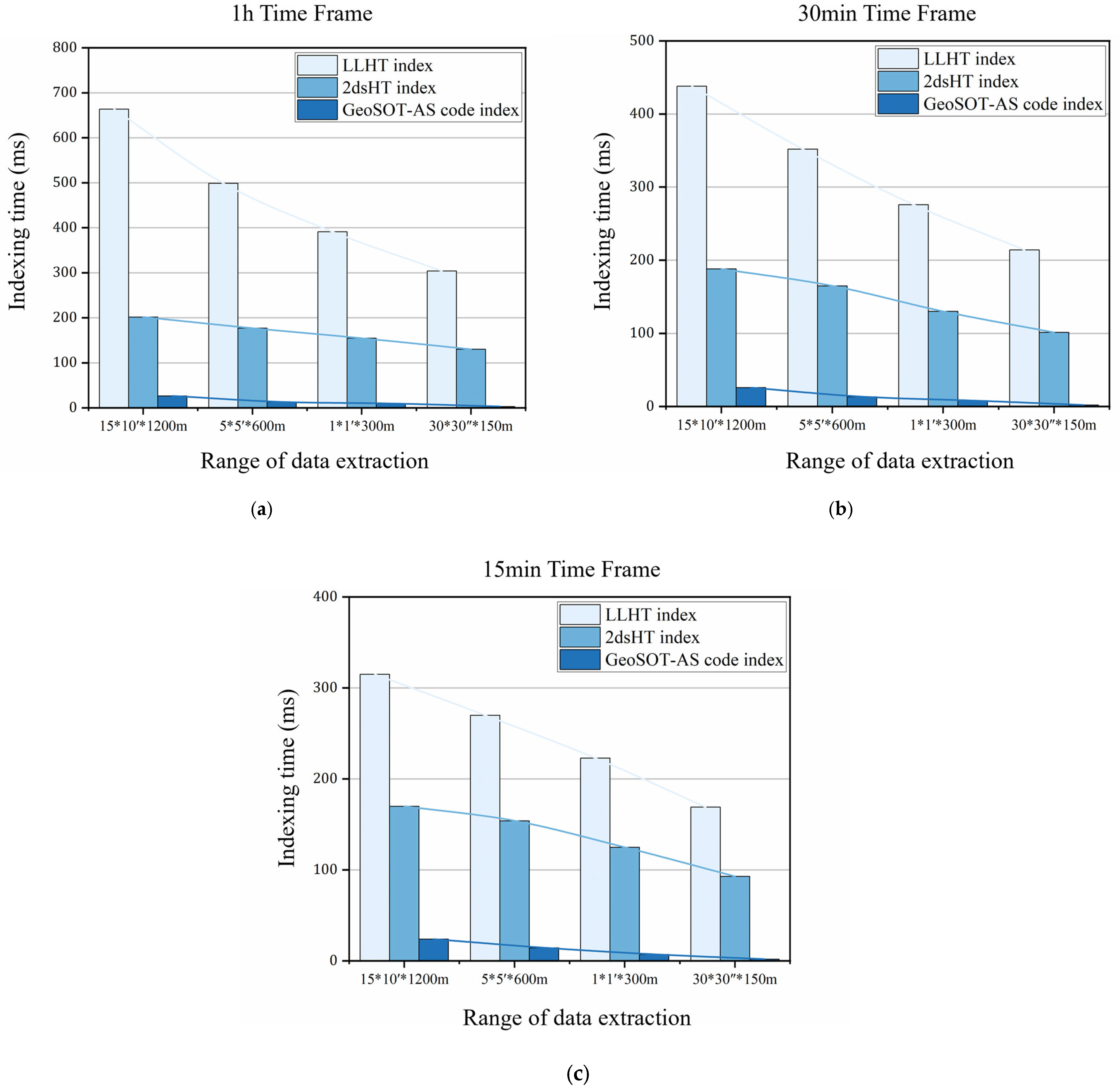
The area of interest is still randomly selected, and the ADS-B point data source is searched for within the corresponding stratification scale with 113.304006° E, 23.385286° N functioning as the lower left corner point, and the planes corresponding to 15∗10′, 5∗5′, 1∗1′, and 30∗30″ rectangular envelope space enclosing boxes, and the heights are set to 1200, 600, 300, and 150, according to the stratification rules.

Under the above regional conditions, the indexing query with time interval settings was divided into four time intervals for the experimental query, and the indexing operations were performed for four task durations with five random time starting points and time intervals of 1 h, 30 min, and 15 min. The average time consumption of different methods and their time comparisons are shown in the figure below. This condition, i.e., the indexing tasks with different time intervals are set to judge the effectiveness of the time-coded indexes included in the null field coding.

From the efficiency test results, it was found that the spatiotemporal query response time of each index decreases significantly when the query range increases (i.e., when the spatial range of the index decreases), which matches the empirical amount of the actual experiment. Elsewhere, another aspect of the cross-sectional comparison was that the spatiotemporal query response time tended to decrease when the time interval of the spatiotemporal index was compressed, which is consistent with the overall trend when considering the query volume of the whole data set. The response time is shown in Figure 12.

When comparing longitudinally, it was discovered that the initial approach of constructing a composite spatiotemporal index using LLHT and spatial indices had some disadvantages. Specifically, the query response time was abnormally slow and constituted the longest response time among all types of tasks. The second way of constructing composite spatiotemporal index with 2dsphere spatial index plus highly hierarchical index and time slice was better than the first way of constructing composite spatiotemporal indices. The second type of 2dsHT index, which is a composite spatiotemporal index constructed by using 2dsphere spatial index plus highly hierarchical index and temporal slicing, is tested to be more efficient under different data volumes and is more efficient than the first type of construction. The third spatiotemporal grid-based coding in the index constructed in this way is better than the first two spatiotemporal query performances; moreover, the fluctuation under the condition of index hierarchy change is much smaller than the first two methods, approximating to O(n).

7. Conclusions

The focus of this study was to address the needs of ADS-B data organization management and actual airspace management by utilizing the multi-level dissection methods of the GeoSOT grid model. We redesigned and developed a set of grids in GeoSOT-AS specifically for airspace management. The framework was designed to keep the flight space deformation rate low, with a maximum deformation rate of only 16% in China’s airworthy airspace. This framework is suitable for current ADS-B data organization, which represents air traffic control. Furthermore, we designed the mapping relationship of the ATC information data structure based on this framework and proposed an information management method with the GeoSOT-AS grid code as the primary key. The primary key management based on airspace grid code is more effective in extraction performance under the task requirement of regional ATC information extraction. We designed two typical experiments: point source information extraction at a global time and fixed time period, as well as airspace information extraction in different scale regions. The results confirmed that the information extraction speed efficiency in the framework of ATC region was improved by about 81%.

Our future work will concentrate on specific ATC tasks that utilize the airspace grid, including the implementation of airspace use deployment functions based on the Geo-SOT-AS framework, and the development of space flight plan anti-collision functions using the airspace grid management concept to integrate additional ATC data. Our goal is to establish a comprehensive ATC database, also referred to as the ATC digital map model, which can be used to support a wide range of algorithmic functions for ATC calculation tasks.

References

- Strohmeier, M.; Lenders, V.; Martinovic, I. Security of ADS−B: State of the Art and Beyond; DCS: Huntsville, AL, USA, 2013. [Google Scholar]
- Pollack, J.; Ranganatha, P. Aviation navigation systems security: ADS-B, GPS, IFF. In Proceedings of the International Conference on Security and Management (SAM), Las Vegas, NV, USA, 30 July–2 August 2018. [Google Scholar]
- Li, B.; Zhai, S.; Li, R. R esearch on Air Route Conflict Detection for General Aviation based on ADS-B. In Proceedings of the 3rd International Conference on Robotics Systems and Automation Engineering (RSAE), Paris France, 28–30 May 2021; pp. 70–76. [Google Scholar]
- Vito, D.; Torrano, G. RPAS Automatic ADS-B Based Separation Assurance and Collision Avoidance System Real-Time Simulation Results. Drones 2020, 4, 73. [Google Scholar] [CrossRef]
- Holdsworth, R.; Lambert, J.; Harle, N. Inflight path planning replacing pure collision avoidance, using ADS-B. IEEE Aerosp. Electron. Syst. Mag. 2001, 16, 27–32. [Google Scholar] [CrossRef] [PubMed]
- Ali, B.S. System specifications for developing an Automatic Dependent Surveillance-Broadcast (ADS-B) monitoring system. Int. J. Crit. Infrastruct. Prot. 2016, 15, 40–46. [Google Scholar] [CrossRef]
- Sampigethaya, K.; Poovendran, R. Aviation Cyber–Physical Systems: Foundations for Future Aircraft and Air Transport. Proc. IEEE 2013, 101, 1834–1855. [Google Scholar] [CrossRef]
- Keller, R.M. Ontologies for aviation data management. In Proceedings of the IEEE/AIAA 35th Digital Avionics Systems Conference (DASC), Sacramento, CA, USA, 25–29 September 2016. [Google Scholar]
- Wandelt, S.; Sun, X.; Fricke, H. Ads-bi: Compressed indexing of ads-b data. IEEE Trans. Intell. Transp. Syst. 2018, 19, 3795–3806. [Google Scholar] [CrossRef]
- Wandelt, S.; Sun, X. Efficient Compression of 4D-Trajectory Data in Air Traffic Management. IEEE Trans. Intell. Transp. Syst. 2015, 16, 844–853. [Google Scholar] [CrossRef]
- Rex, J.; Ballard, D.; Garrow, L.A.; Mills, R.W.; Weingart, D. A new GIS database documenting the prevalence of U.S. air service development incentives. J. Air Transp. Manag. 2022, 98, 102148. [Google Scholar] [CrossRef]
- Zhu, Y.; Chen, Z.; Pu, F.; Wang, J. Development of digital airspace system. Strateg. Study Chin. Acad. Eng. 2021, 23, 135–143. [Google Scholar] [CrossRef]
- Yongwen, Z.H.U.; Fan, P.U. Principle and application of airspace spatial grid identification. J. Beijing Univ. Aeronaut. Astronaut. 2021, 47, 2462–2474. [Google Scholar] [CrossRef]
- Yongwen, Z.H.U.; Hua, X.I.E.; Fan, P.U. Research of airspace gridding method and its application in air traffic management. Adv. Aeronaut. Sci. Eng. 2021, 12, 12–24. [Google Scholar]
- Xue, M. Airspace sector redesign based on Voronoi diagrams. J. Aerosp. Comput. Inf. Commun. 2009, 6, 624–634. [Google Scholar] [CrossRef]
- Tang, J.; Alam, S.; Lokan, C.; Abbass, H.A. A multi-objective approach for Dynamic Airspace Sectorization using agent based and geometric models. Transp. Res. Part C Emerg. Technol. 2012, 21, 89–121. [Google Scholar] [CrossRef]
- Li, J.; Wang, T.; Savai, M.; Hwang, I. Graph-based algorithm for dynamic airspace configuration. J. Guid. Control Dyn. 2010, 33, 1082–1094. [Google Scholar] [CrossRef]
- Sergeeva, M.; Delahaye, D.; Mancel, C.; Vidosavljevic, A. Dynamic airspace configuration by genetic algorithm. J. Traffic Transp. Eng. 2017, 4, 300–314. [Google Scholar] [CrossRef]
- Alipio, J.; Castro, P.; Kaing, H.; Shahid, N.; Sherzai, O.; Donohue, G.; Grundmann, K. Dynamic airspace super sectors (DASS) as high-density highways in the sky for a new US air traffic management system. In Proceedings of the IEEE Systems and Information Engineering Design Symposium 2003, Charlottesville, VA, USA, 24–25 April 2003; IEEE: Piscataway, NJ, USA, 2003. [Google Scholar]
- Yousefi, A.; Donohue, G.L.; Sherry, L. High-volume tube-shape sectors (HTS): A network of high capacity ribbons connecting congested city pairs. In Proceedings of the 23rd Digital Avionics Systems Conference (IEEE Cat. No. 04CH37576), Salt Lake City, UT, USA, 28 October 2004; IEEE: Piscataway, NJ, USA, 2004. [Google Scholar]
- Hering, H. Air traffic freeway system for Europe. In Eurocontrol Experimental Centre EEC Note; (20/05); European Organisation for the Safety of Air Navigation: Brussels, Belgium, 2005. [Google Scholar]
- ICAO. Annex 4: Aeronautical Charts; ICAO: Montreal, QC, Canada, 2009. [Google Scholar]
- Chang, F.; Dean, J.; Ghemawat, S.; Hsieh, W.C.; Wallach, D.A.; Burrows, M.; Chandra, T.; Fikes, A.; Gruber, R.E. Bigtable. ACM Trans. Comput. Syst. 2008, 26, 1–26. [Google Scholar] [CrossRef]
- Karimi, H.A.; Roongpiboonsopit, D.; Wang, H. Exploring Real-Time Geoprocessing in Cloud Computing: Navigation Services Case Study. Trans. GIS 2011, 15, 613–633. [Google Scholar] [CrossRef]
- Whitman, R.; Park, M.B.; Ambrose, S.M.; Hoel, E.G. Spatial indexing and analytics on Hadoo. In Proceedings of the 22nd ACM SIGSPATIAL International Conference on Advances in Geographic Information Systems, Dallas, TX, USA, 4–7 November 2014; pp. 73–82. [Google Scholar]
- Yu, J.; Wu, J.; Sarwat, M. GeoSpark: A cluster computing framework for processing large-scale spatial data. In Proceedings of the 23rd SIGSPATIAL International Conference on Advances in Geographic Information Systems, Seattle, WA, USA, 3 November 2015; pp. 1–4. [Google Scholar]
- Khoshafian, S.; Copeland, G.; Jagodits, T.; Boral, H.; Valduriez, P. A Query Processing Strategy for the Decomposed Storage Model. In Proceedings of the 3rd International Conference on Data Engineering, Los Angeles, CA, USA, 3–5 February 1987; IEEE Computer Society: Washington, DC, USA, 1987; pp. 636–643. [Google Scholar]
- Boncz, P.A.; Kersten, M.L. MIL primitives for querying a fragmented world. VLDB J. 1999, 8, 101–119. [Google Scholar] [CrossRef] [Green Version]
- Eldawy, A.; Mokbel, M.F.; Alharthi, S.; Alzaidy, A.; Tarek, K.; Ghani, S. SHAHED: A MapReduce-based system for querying and visualizing spatio-temporal satellite data. In Proceedings of the 2015 IEEE 31st International Conference on Data Engineering, Seoul, Republic of Korea, 13–17 April 2015. [Google Scholar]
- Ma, Q.; Yang, B.; Qian, W.; Zhou, A. Query processing of massive trajectory data based on MapReduce. In Proceedings of the First International Workshop on Cloud Data Management, Hong Kong, China, 2 November 2009; pp. 9–16. [Google Scholar]
- Shang, Z.; Li, G.; Bao, Z. DITA: A Distributed In-Memory Trajectory Analytics System. In Proceedings of the 2018 International Conference on Management of Data, Houston, TX, USA, 10–15 June 2018; pp. 1681–1684. [Google Scholar]
- Hoel, E.; Marsh, B.G.; Park, M.B.; Hoel, E.G. Spatio-Temporal Join on Apache Spark. ACM Trans. Spat. Algorithms Syst. 2017, 5, 1–28. [Google Scholar]
- Tan, H.; Luo, W.; Ni, L. CloST: A hadoop-based storage system for big spatio-temporal data analytics. In Proceedings of the 21st ACM International Conference on Information and Knowledge Management, Maui, HI, USA, 29 October–2 November 2012; pp. 2139–2143. [Google Scholar]
- Xie, X.; Mei, B.; Chen, J.; Du, X.; Jensen, C.S. Elite: An elastic infrastructure for big spatiotemporal trajectories. VLDB J. 2016, 25, 473–493. [Google Scholar] [CrossRef]
- Cary, A.; Sun, Z.; Hristidis, V.; Rishe, N. Experiences on Processing Spatial Data with MapReduce. In Scientific and Statistical Database Management: 21st International Conference, SSDBM 2009 New Orleans, LA, USA, 2–4 June 2009; Springer: Berlin/Heidelberg, Germany, 2009; Volume 5566, pp. 302–319. [Google Scholar]
- Eldawy, A.; Alarabi, L.; Mokbel, M. Spatial partitioning techniques in SpatialHadoop. Proc. VLDB Endow. 2015, 8, 1602–1605. [Google Scholar] [CrossRef] [Green Version]
- Han, W.S.; Kim, J.; Lee, B.S.; Tao, Y.; Rantzau, R.; Markl, V. Cost-Based Predictive Spatiotemporal Join. IEEE Trans. Knowl. Data Eng. 2009, 21, 220–233. [Google Scholar]
- Fox, A.; Eichelberger, C.; Hughes, J.; Lyon, S. Spatio-temporal indexing in non-relational distributed databases. In Proceedings of the IEEE International Conference on Big Data, Silicon Valley, CA, USA, 6–9 October 2013. [Google Scholar]
- Cheng, C.; Tong, X.; Chen, B.; Zhai, W. A Subdivision Method to Unify the Existing Latitude and Longitude Grids. ISPRS Int. J. Geo-Inf. 2016, 5, 161. [Google Scholar] [CrossRef] [Green Version]
- Hou, K.; Cheng, C.; Chen, B.; Zhang, C.; He, L.; Meng, L.; Li, S. A Set of Integral Grid-Coding Algebraic Operations Based on GeoSOT-3D. ISPRS Int. J. Geo-Inf. 2021, 10, 489. [Google Scholar] [CrossRef]
- Li, S.; Hou, K.; Cheng, C.; Li, S.; Chen, B. A Space-Interconnection Algorithm for Satellite Constellation Based on Spatial Grid Model. Remote Sens. 2020, 12, 2131. [Google Scholar] [CrossRef]
- Tong, X.; Cheng, C.; Wang, R.; Ding, L.; Zhang, Y.; Lai, G.; Wang, L.; Chen, B. An efficient integer coding index algorithm for multi-scale time information management. Data Knowl. Eng. 2019, 119, 123–138. [Google Scholar] [CrossRef]
- Olive, X. Traffic, a toolbox for processing and analysing air traffic data. J. Open Source Softw. 2019, 4, 1518. [Google Scholar] [CrossRef] [Green Version]
Figure 1.
Introduction to ADS-B system.
Figure 2.
(a) 6 × 4° profile structure of the primary grid (1st level profile); (b) The order of the codes represented by the space-filling curves (2nd and 3rd level profile); (c) Aeronautical maps of the corresponding scale.
Figure 3.
Multi-level profiling process of GeoSOT-AS planar dimension (4th–11th level profile).
Figure 4.
Four different types of fill curves: (a) 2 × 3 profiling; (b) 2 × 2 profiling; (c) 3 × 2 profiling; (d) 5 × 5 profiling.
Figure 5.
Planar dimensional coding scale and bit representation.
Figure 6.
Height division and coding method: (a) flight height level division; (b) binary tree encoding structure of height.
Figure 7.
Data representation under GeoSOT-AS model.
Figure 8.
ADS-B data extraction algorithm flow chart.
Figure 9.
Geographical distribution of data: (a) the distribution of planar latitude and longitude; (b) height range distribution; (c) time range distribution.
Figure 10.
Analysis of shape change law with height: (a) grid scale variation; (b) capacity variation.
Figure 11.
Comparison of time spent on the spatiotemporal range indexing for a fixed time: (a) actual time consumption for the indexing operation; (b) time consumption for the Index Scan process.
Figure 12.
Regional and time segment data extraction performance test: (a) set the time frame to 1 h; (b) set the time frame to 30 min; (c) set the time frame to 15 min.