
Tactical Conflict Solver Assisting Air Traffic Controllers Using Deep Reinforcement Learning

1
College of Civil Aviation, Nanjing University of Aeronautics and Astronautics, Nanjing 211106, China
2
Jiangsu Sub-Bureau of East China Regional Air Traffic Management Bureau, Civil Aviation Administration of China, Nanjing 211113, China
*
Author to whom correspondence should be addressed.
Aerospace 2023, 10(2), 182; https://doi.org/10.3390/aerospace10020182
Submission received: 22 December 2022
/
Revised: 4 February 2023
/
Accepted: 13 February 2023
/
Published: 15 February 2023
(This article belongs to the Special Issue Advances in Air Traffic and Airspace Control and Management)
Abstract
:To assist air traffic controllers (ATCOs) in resolving tactical conflicts, this paper proposes a conflict detection and resolution mechanism for handling continuous traffic flow by adopting finite discrete actions to resolve conflicts. The tactical conflict solver (TCS) was developed based on deep reinforcement learning (DRL) to train a TCS agent with the actor–critic using a Kronecker-factored trust region. The agent’s actions are determined by the ATCOs’ instructions, such as altitude, speed, and heading adjustments. The reward function is designed in accordance with air traffic control regulations. Considering the uncertainty in a real-life situation, this study characterised the deviation of the aircraft’s estimated position to improve the feasibility of conflict resolution schemes. A DRL environment was developed with the actual airspace structure and traffic density of the air traffic operation simulation system. Results show that for 1000 test samples, the trained TCS could resolve 87.1% of the samples. The conflict resolution rate decreased slightly to 81.2% when the airspace density was increased by a factor of 1.4. This research can be applied to intelligent decision-making systems for air traffic control.
1. Introduction
Before the COVID-19 pandemic, the scale of civil aviation transportation showed rapid growth. Compared to 2018, daily flights in Europe increased by 8% in 2019 [1]. Nearly 11.5 million commercial flights were completed in the United States in 2019 [2]. In 2019, transport airlines in the Chinese civil aviation industry performed 4.966 million take-offs, indicating an annual increase of 5.8% [3]. Although air traffic has decreased during the COVID-19 pandemic, it will continue to grow as the temporary crisis passes.
Identification and resolution of possible conflicts by air traffic controllers (ATCOs) alone is feasible with the current traffic flow. However, as traffic flows increase, so do the number of conflicts and the frequency with which they occur. This will result in an increased workload for ATCOs, which could lead to traffic flow restrictions and, therefore, flight delays, in addition to affecting flight safety. From this perspective, decision support technologies that can automatically perform conflict detection and provide ATCOs with appropriate conflict resolution (CR) schemes and reduce the workload on ATCOs.
Decision support systems with conflict detection and resolution functions can be broadly classified into two categories. One category is ground-based systems (primarily designed to assist ATCOs in their decision making), such as the Centre/TRACON Automation System (CTAS) [4], the User Request Evaluation Tool (URET) [5], and En Route Automation Modernization (ERAM) [6]. Another category is airborne systems (primarily designed to aid in aircraft decision making), such as the Airborne Separation Assurance System (ASAS) [7], the Traffic Collision Avoidance System (TCAS) [8], the Airborne Collision Avoidance System (ACAS) [9], and ACAS Xu [10]. Different assisted decision-making targets have different requirements for mechanisms and algorithms. Assisting ATCOs is concerned with acceptance of schemes by ATCOs and air traffic control (ATC) regulators. Existing decision support systems need to be improved in terms of handling specific tasks and scenarios. The higher level of ATC automation requires automation to adapt to a broad range of scenarios and tasks while giving the human operator appropriate action advice [11]. Therefore, this work uses the deep reinforcement learning (DRL) method to implement a core function in decision support systems, i.e., conflict resolution, to improve the CR model’s intelligence level.
This study aims to assist ATCOs in resolving tactical conflicts. ‘Tactical’ here corresponds to the second level of ICAO’s conflict management ‘separation regulations’ [12]. Based on ATCOs’ decision-making habits and dynamic decision-making process in CR, this work designs a conflict detection and resolution (CD&R) mechanism capable of handling continuous traffic flow under the CD&R framework. The tactical conflict solver (TCS) agent is trained in the actor–critic using a Kronecker-factored trust region (ACKTR), taking into account multiple constraints, such as ATC regulations, uncertainty in the real environment, and the real airspace environment. The DRL environment was developed based on the Air Traffic Operations Simulation System (ATOSS). Depending on the real-time situation, the TCS can resolve conflicts in real 3D airspace with high quality by using altitude, speed, or heading adjustments used by ATCOs and taking into account the operations of other aircraft.
The remainder of this paper is organized as follows. Section 2 presents a description of the CD&R framework and mechanism, the construction of a Markov decision process (MDP) model for resolving two-aircraft conflicts, and a description of the training method. Section 3 presents a description of the analysis of the experimental results and a discussion. Section 4 summarises the research and provides an outlook on the future scope of research.
2. Previous Related Works
Academic efforts are underway to address CR problems. Reviews of CR problems can be found in several reports [13,14,15]. The main approaches to solving CR problems include optimal control methods, mathematical programming methods, swarm intelligence optimisation or search methods, and machine learning methods. Soler et al. [16] considered fuel-optimal conflict-free trajectory planning as a hybrid optimal control problem. Matsuno et al. [17] considered wind certainty and solved the CR problem using the stochastic near-optimal control method. Liu et al. [18] further considered constructive weather areas and proposed a stochastic optimal control algorithm for collision avoidance. The CR schemes obtained using optimal control methods are generally a trajectory composed of continuous position points of the aircraft, which is quite different from the scheme of ATCOs. Among mathematical programming methods, most studies have employed mixed-integer nonlinear programming (MINLP) or mixed-integer linear programming (MILP) to establish mathematical models [19,20,21,22,23]. In addition, some studies established general nonlinear models or used a two-step optimisation approach [24,25]. Mathematical programming methods allow customised models to be built and globally solved for different CR problems. However, it is difficult to describe the complex motion processes of aircraft and the variable airspace operating environment and constraints. Swarm intelligence optimisation or search methods describe the airspace operating environment through simulation. This approach can consider a variety of nonlinear constraints. In 1996, Durand et al. [26] used the genetic algorithm (GA) for CR. Ma et al. [27] abstracted airspace as a grid and studied the use of the GA to solve the CR problem in the context of free flight. Emami et al. [28] studied multiagent-based CR problems using the particle swarm optimisation (PSO) algorithm. Sui et al. [29] used the Monte Carlo tree search (MCTS) algorithm to solve the CR problem in high-density airspace.
Recently, many researchers have attempted to use machine learning methods, such as supervised learning and DRL, to solve CR problems. Machine learning methods are fast and have high intelligence levels. Supervised learning methods use datasets to construct and train models to map conflict scenarios and CR schemes [30,31,32]. DRL methods focus on enabling a self-learning model with human-like behaviour. According to the object of auxiliary decision making, the current research can be divided into that focused on assisting the decision making of ATCOs and that assisting the decision making of aircraft. The research on assisting ATCOs’ decision-making is described as follows. Based on a free-flight context, Wang et al. [33] considered the turning radius of aircraft, used the two-dimensional heading adjustment to resolve conflicts, and matched the actual ATC mode by limiting the number of heading angle changes. They used the K-control actor–critic (KCAC) algorithm to train the agent. Alam et al. [34,35] ordered aircraft to perform a similar ‘dog leg’ manoeuvre to resolve conflicts. The deep deterministic policy gradient (DDPG) was used to train the agent, considering the uncertainty in executing ATCOs’ commands by the aircraft [34]. The model achieved a resolution rate of approximately 87% for different levels of uncertainty. The difference between the CR schemes given by real ATCOs and the agent was measured and added to the reward function to make the schemes given by the agent and ATCOs similar [35]. Sui et al. [36] defined the type of multiaircraft conflict based on the existing operation mode. They trained multiagents to resolve multiaircraft conflicts using the independent deep Q network (IDQN) algorithm. The model used a maximum of three actions to resolve conflicts and achieved a resolution rate of 85.71%. The types of actions included speed, altitude, and heading adjustments. Dalmau et al. [37] presented a recommendation tool based on multiagent reinforcement learning (MARL) to support ATCOs. The policy function was trained by gathering experiences in a controlled simulation environment. Agents deployed aircraft in two dimensions.
Research on aircraft-assisted decision making includes the following. Wei et al. [38,39] focused on the traversing of an en route sector with multiple intersections by different numbers of aircraft. They established a deep multiagent reinforcement learning framework to achieve the autonomous interval maintenance of the aircraft. Their model was scalable and supported the deployment of different numbers of aircraft. The aircraft used the speed adjustment action at an interval of 12 s to resolve conflicts. The framework used the proximal policy optimisation (PPO) algorithm, incorporating a long short-term memory network to ensure the model’s scalability [38]. In another study [39], the same authors proposed a scalable autonomous separation assurance framework and verified its effectiveness in high-density airspace. Isufaj et al. [40] used a multiagent deep deterministic policy gradient (MADDPG) to train two agents, representing each aircraft in a two-aircraft conflict. The agents used heading and speed adjustments to resolve conflicts and executed adjustments every 15 s. The action space was continuous. Ribeiro et al. [41,42] focused on the operating environment of UAVs. They combined DDPG and the modified voltage potential (MVP) method to improve the CR capability of UAVs under high-traffic densities.
To compare the characteristics of the aforementioned CR methods, we reviewed the above literature, as shown in Table 1. Assisting ATCOs means that the controller can execute the CR scheme of the model output under the current ATC mode, which usually requires the CR manoeuvres to be discrete in terms of execution time and magnitude. CR manoeuvres are 2D for conflict resolution via horizontal manoeuvres and 3D for conflict resolution via stereo manoeuvres (usually including altitude adjustment). Uncertainty refers to the uncertainty of flight in the real environment, for example, wind uncertainty. The supervised learning and DRL methods have a solution time of less than 1 s. Although much literature does not show the solution time, the supervised learning and DRL methods use neural networks to build mappings to obtain the CR scheme, so the solution time is similar. The solution time for other methods ranges from a few seconds to several thousand seconds. As the complexity of the scenario increases, the solution time also increases, easily exceeding the solution time allowed for tactical conflict resolution. There are three papers describing complete and detailed CD&R mechanisms. However, the CD&R mechanism in [29] cannot handle continuous traffic flow; in [38,39], aircraft were assisted in decision making rather than ATCOs. This work, therefore, deepens the study of the CD&R mechanism based on the need to assist ATCOs in resolving tactical conflicts and dealing with continuous traffic flow. Furthermore, this work uses discrete 3D manoeuvres to assist ATCOs in resolving tactical conflicts within the current ATC mode and regulations, taking into account flight uncertainty and ensuring a stable solution time of a few seconds.
In this work, we propose a receding horizontal control CD&R mechanism that can handle continuous traffic flow to assist ATCOs in conflict resolution. To improve the intelligence level and computational speed, the TCS agent is trained using the DRL method, considering the flight uncertainty and the existing ATC mode. The TCS agent uses the altitude, speed, and heading adjustments used by ATCOs daily to resolve tactical conflicts. The DRL environment was developed based on a high-fidelity airspace simulation system to ensure that the training environment is similar to the real environment. This paper focuses on CD&R under common flight conditions and therefore does not consider meteorological impacts, which will be considered in future studies.
3. Methodology
3.1. Conflict Detection and Resolution Framework
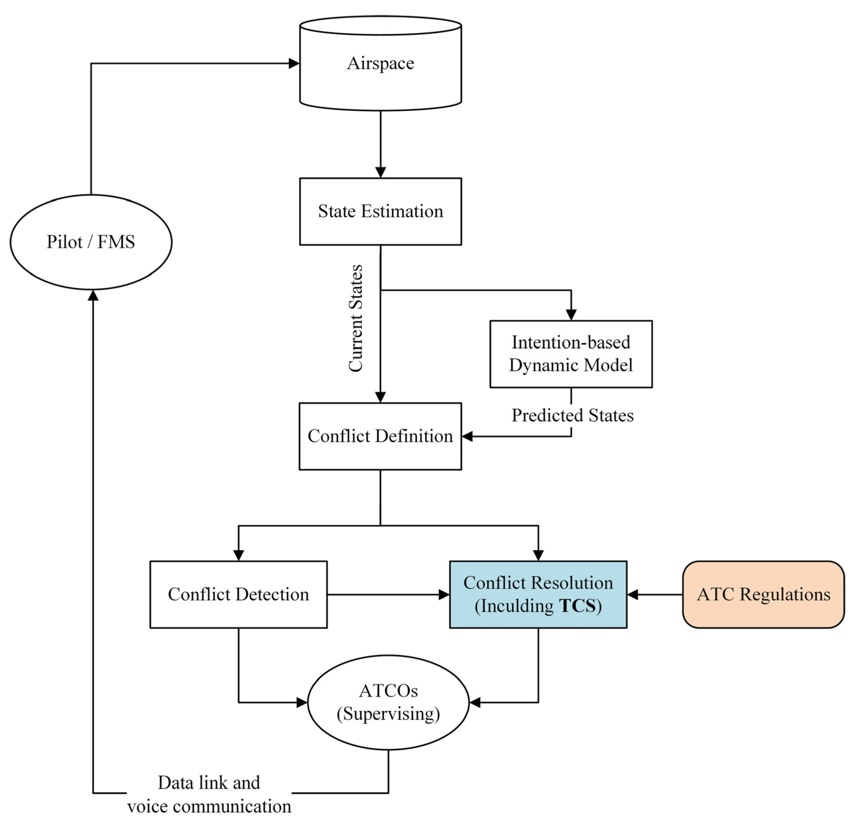
Based on the CD&R framework for assisting ATCOs’ decision-making proposed by Kuchar et al. [13], relevant modules are refined, as shown in Figure 1. The state estimation module observes the airspace and obtains an estimate of the current traffic situation, which is then passed to the intention-based dynamic model to estimate the future state of the airspace. The conflict detection module generates conflict information based on conflict definitions. The conflict resolution module generates CR instructions based on ATC regulations.
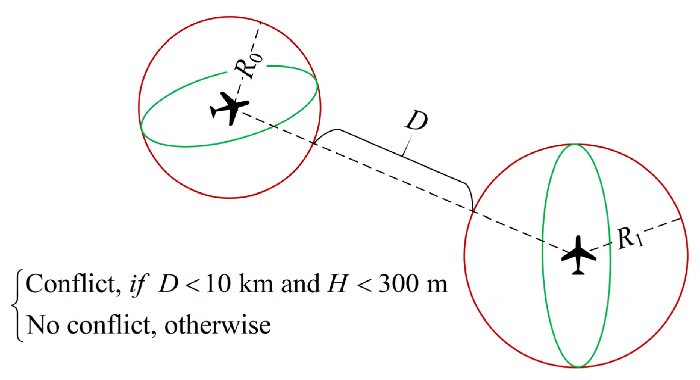
In this paper, a flight conflict is defined as a case in which the horizontal separation between two aircraft is less than 10 km and the vertical separation is less than 300 m at a particular time. The ATC regulations reflect that (1) the CR instructions should be the daily CR instructions used by ATCOs and (2) the CR instructions should adjust the flight state of the aircraft to ensure that parameters such as the speed, rate of climb, and acceleration are consistent with the aircraft dynamics. Therefore, the CR instructions in this study include altitude, speed, and heading adjustments. According to the ICAO document [43] and our previous study [36], the altitude adjustment is set to 300 m, the speed adjustment is 10 kt, and the heading adjustment is obtained using the route offsets. The offset turning angle is 30°, and the offset distance is 6 nm from the original route.
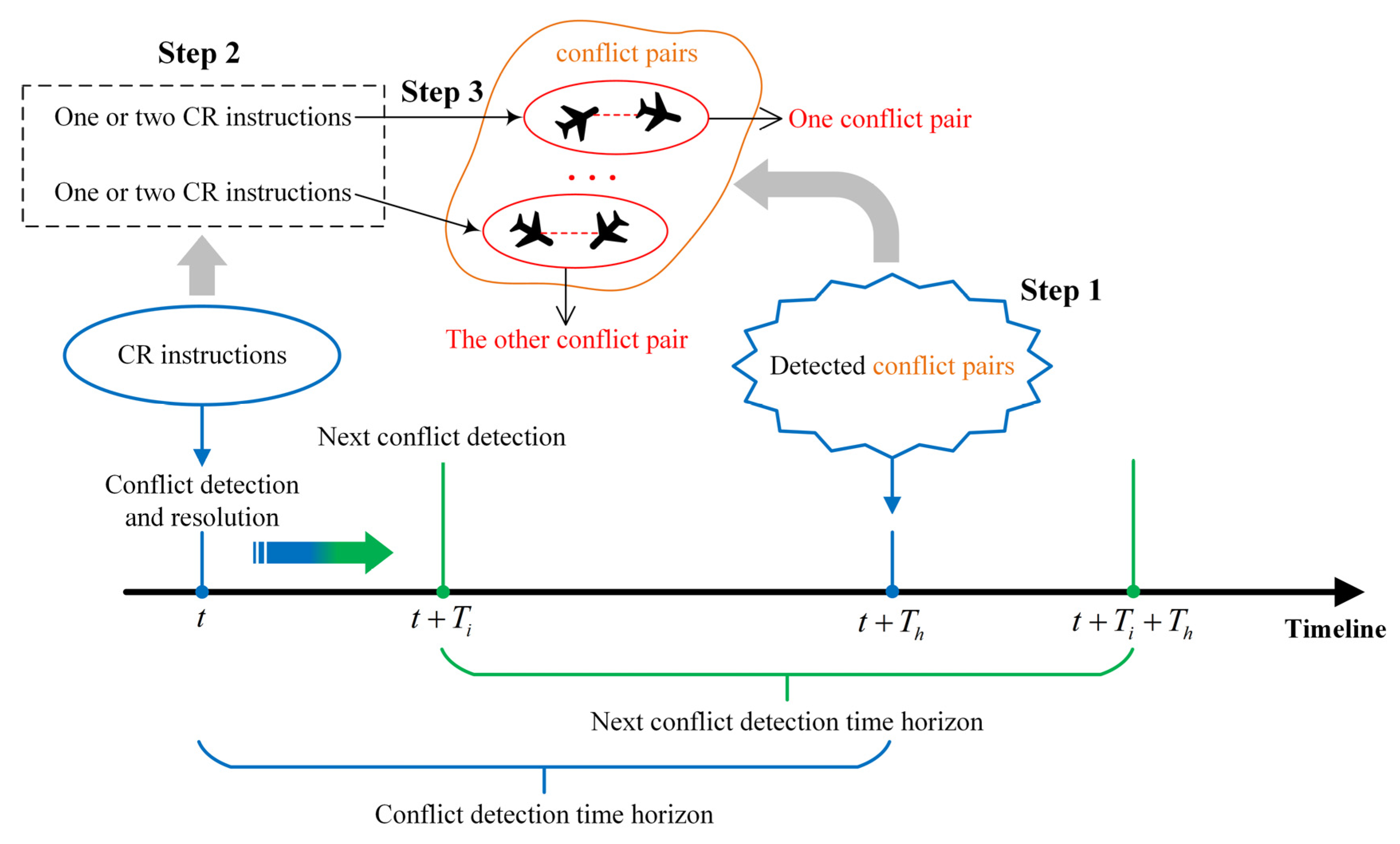
Based on the need for continuous traffic flow, a forward rolling CD&R mechanism is proposed, as shown in Figure 2. In the figure, is the current moment, is the time interval for conflict detection, and is the time horizon of forwarding detection in conflict detection. Referring to the review reported in [14], tactical conflict resolution in this study is defined as the resolution of a two-aircraft conflict that exists after 6 min. Therefore, set . Theoretically, should be set small enough so that the high frequency of conflict detection ensures that no conflicts are missed. However, the smaller the , the greater the computational load. Based on the flight speed of the aircraft and the results of several experiments, this work sets .
- Step 1: Conflict detection. At , the proposed mechanism detects whether there are conflict pairs at (a conflict pair is an aircraft conflict involving two aircraft). If there are no conflict pairs, the subsequent conflict detection is performed after . If there are conflict pairs, the conflict resolution session is initiated.
- Step 2: Conflict resolution. One or two CR instructions are generated for each conflict pair in turn at time (if a single CR instruction cannot resolve the conflict pair, two CR instructions are generated for each of the conflicting aircraft to execute).
- Step 3: Scheme selection. Let CONDITION be the condition for successfully resolving a conflict pair, i.e., the given CR instructions need to ensure that there is no conflict between the two aircraft in the conflict pair at and that there is no conflict between the two conflicting aircraft and the neighbouring aircraft at . CONDITION involves the time horizon and neighbouring aircraft in order to avoid secondary conflicts. If the CR instructions satisfy CONDITION , they are sent to the controller; otherwise, the controller resolves the conflict manually. The subsequent conflict detection is then started after .For example, at , the detection conflicts occur at : aircraft A and B are in conflict, and aircraft A and C are in conflict. Thus, two conflict pairs can be formed: A–B and A–C. Depending on the severity of the conflict pairs (measured, for example, by the distance between conflicting aircraft), A–B is assumed to be a high priority, and A–C is the next highest priority. At , CR instructions are first generated to resolve the A–B conflict pair, and then additional CR instructions are generated to resolve the A–C conflict pair. It is then determined whether the CR instructions satisfy CONDITION to determine whether they can be sent to the controller. Finally, after , the subsequent conflict detection is started.
3.2. Conflict Resolution Model
3.2.1. Conflict Resolution Model Based on Markov Decision Process
Let the TCS be the agent and the airspace be the environment. Let time be the moment when the resolution of a conflict pair begins. Let the two aircraft in the conflict pair be and .
- Based on the state (), the TCS agent generates and executes an action () (giving the CR instruction corresponding to ) and then receives the reward (). contains the airspace situation at and the predicted airspace situation a while after for the agent to receive sufficiently comprehensive information. The trajectory prediction determines whether CONDITION is satisfied after executes the CR instruction. If the condition is met, the conflict pair is successfully resolved, and the terminal state is reached.
- Suppose the conflict pair is not successfully resolved. In that case, the state is transferred from to ( contains the airspace situation at and the predicted airspace situation for a while after the CR instruction has been executed by ). The TCS agent generates and executes an action () (giving the CR instruction corresponding to ) based on the latest state () and then receives the reward (). Subsequently, a terminal state is reached. If CONDITION is satisfied, the TCS agent successfully resolves the conflict pair; otherwise, the conflict resolution fails.
According to the above description, and only depend on and , not on earlier states and actions; that is, the agent–environment interface of the discrete time satisfies the Markov property. Therefore, the CR model can be modelled as a discrete-time MDP, and the DRL method can be used to solve the MDP.
3.2.2. MDP Description
The MDP is represented by the tuple , where is the state space, is the action space, is the state transition function, is the reward space, and is the discount factor. The MDP established in this study involves complex motion processes in the aircraft, making it difficult to build an accurate dynamic model for the environment, so the model-free method is used. is described in Section 3.2.
- (1)
- State space
The midpoint of the line joining the two aircraft in the conflict pair is defined as the conflict point. After a conflict pair is detected, the 200 × 200 × 6 km cuboid airspace centred on the conflict point is used to describe the state of the current conflict scenario. Because CONDITION involves a time horizon of after the occurrence of the conflict pair, is set to be the 200 × 200 × 6 km cuboid airspace situation from time to time ( is the moment at which the resolution of the conflict pair begins). The airspace situation at is obtained by direct observation of the airspace, whereas the airspace situation at other times is obtained by prediction. With 180 s as the time interval, is given by Equation (1) and can be represented as a vector, where , the components of which represent the longitude, latitude, altitude, and time of occurrence of the conflict point, respectively.
where:
where is the information of the th aircraft in the cuboid airspace. is expressed as:
where , , , , , , , and are the longitude, latitude, altitude, climb rate, horizontal speed, heading, aircraft type (represented by serial number), and the length of the major axis of the confidence ellipse (see Section 3.3.2) of the th aircraft at time . The 1st aircraft is the aircraft receiving the CR instruction, the 2nd aircraft is that with the closest European distance to the 1st aircraft, the 3rd aircraft is that with the next closest European distance to the 1st aircraft, etc. Statistically, the number of aircraft in the 200 × 200 × 6 km cuboid airspace is generally no more than 20 (see Section 3.1), so a maximum value of 30 is set. If there are fewer than 30 aircraft, then the remaining is represented as an all-0 vector. Minimum–maximum normalization is applied to .
- (2)
- Action space
Action space is a collection of actions that the TCS agent can execute. An action represents a CR instruction given by the TCS to an aircraft in the conflict pair. An action (i.e., a CR instruction) is a two-dimensional vector , where denotes altitude, speed, and heading adjustments, and represents the waiting time, that is, the time from the beginning of the resolution of a conflict pair to the actual execution of the adjustment by aircraft. The waiting time enables the adjustment to be executed appropriately. The action space is shown in Table 2. The size of the action space is therefore .
- (3)
- Reward function
The reward function guides the agent towards learning in a direction that yields higher rewards. In this work, the reward function is constructed manually based on the advice of experienced air traffic controllers and it is designed considering the following factors.
- (a)
- The primary goal is to ensure that the conflict pair is resolved; therefore, if it succeeds in resolving the conflict pair, the agent should be rewarded heavily. Conversely, if it fails, it should be given a substantial penalty. A conflict resolution failure occurs when the TCS agent cannot satisfy condition , even after giving CR instructions to the two aircraft in the conflict pair. Accordingly, the reward function () can be expressed as:where the constant is .
- (b)
- The actions given by the TCS agent must be executable. If these actions breach the ATC regulations, the agent will be punished; otherwise, it will be rewarded. The ATC regulations are defined in the second paragraph of Section 3.1. Therefore, the reward function is expressed as:where the constant is . The value of should be set lower than that of because the primary goal is to resolve the conflict pair.
- (c)
- Let be the number of conflicts between the aircraft in the conflict pair plus the number of conflicts between the aircraft in the conflict pair and the neighbouring aircraft during ; then:where the negative coefficient is . By punishing the agent with , the agent can learn to reduce conflicts in the future and improve its ability to satisfy condition .
In summary, the total reward function for the training is expressed as:
3.3. Training Environment
3.3.1. Conflict Scenario Samples
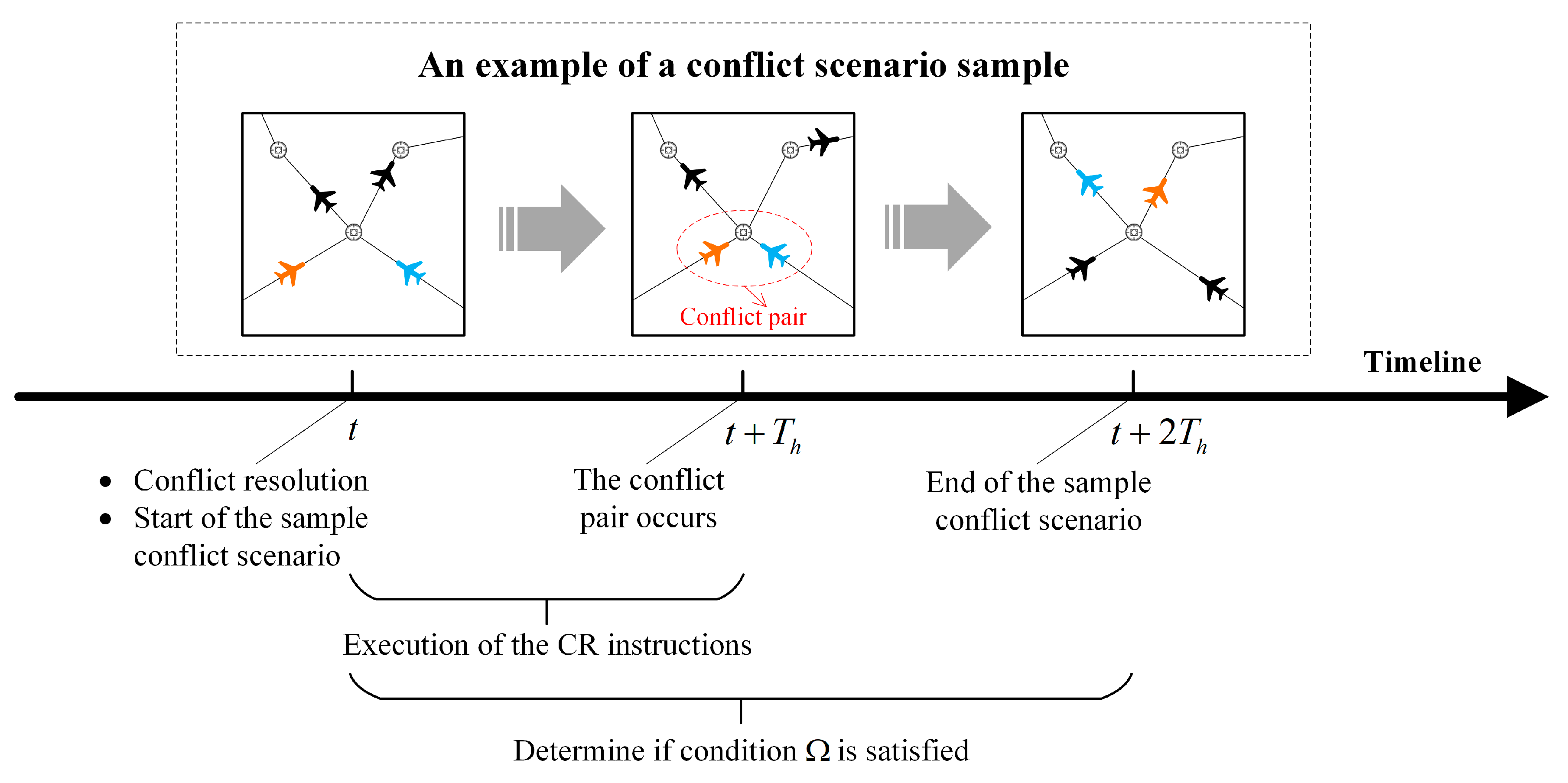
Using DRL to train the TCS agent requires a large number of conflict scenario samples for the dataset. The ability of the CR scheme generated by the TCS needs to be trained to satisfy condition , which involves a time horizon of . Therefore, the conflict scenario sample contains only a time horizon of . As shown in Figure 3, a conflict scenario sample starts at before the conflict pair occurs and ends at after the conflict pair occurs, involving a square of actual airspace with side length . The conflict scenario sample in Figure 3 shows two aircraft associated with the conflict pair (orange and blue) and several neighbouring aircraft (black), which fly along the route according to their flight plans. After loading the conflict scenario sample, the conflict between orange and blue aircraft is detected at , and resolution of that conflict is initiated at . The scenario sample is then run up to to verify that the CR scheme can successfully resolve the conflict pair (i.e., to determine whether condition is met).
In each CD&R process, there is no conflict during (as conflicts in this time horizon have already been resolved in the previous CD&R process). Therefore, the constructed conflict scenario samples must also satisfy this condition. To improve the efficiency of constructing the samples, the condition for generating an adequate sample is weakened as follows. Consider the case in the square airspace where there exists a conflict pair at , and this conflict pair first occurs during . The two aircraft involved in this conflict pair are not in conflict with the neighbouring aircraft in the airspace during . Subsequently, a conflict scenario sample is resolved when and only when the conflict pair in this sample is resolved.
3.3.2. Uncertainty of Prediction
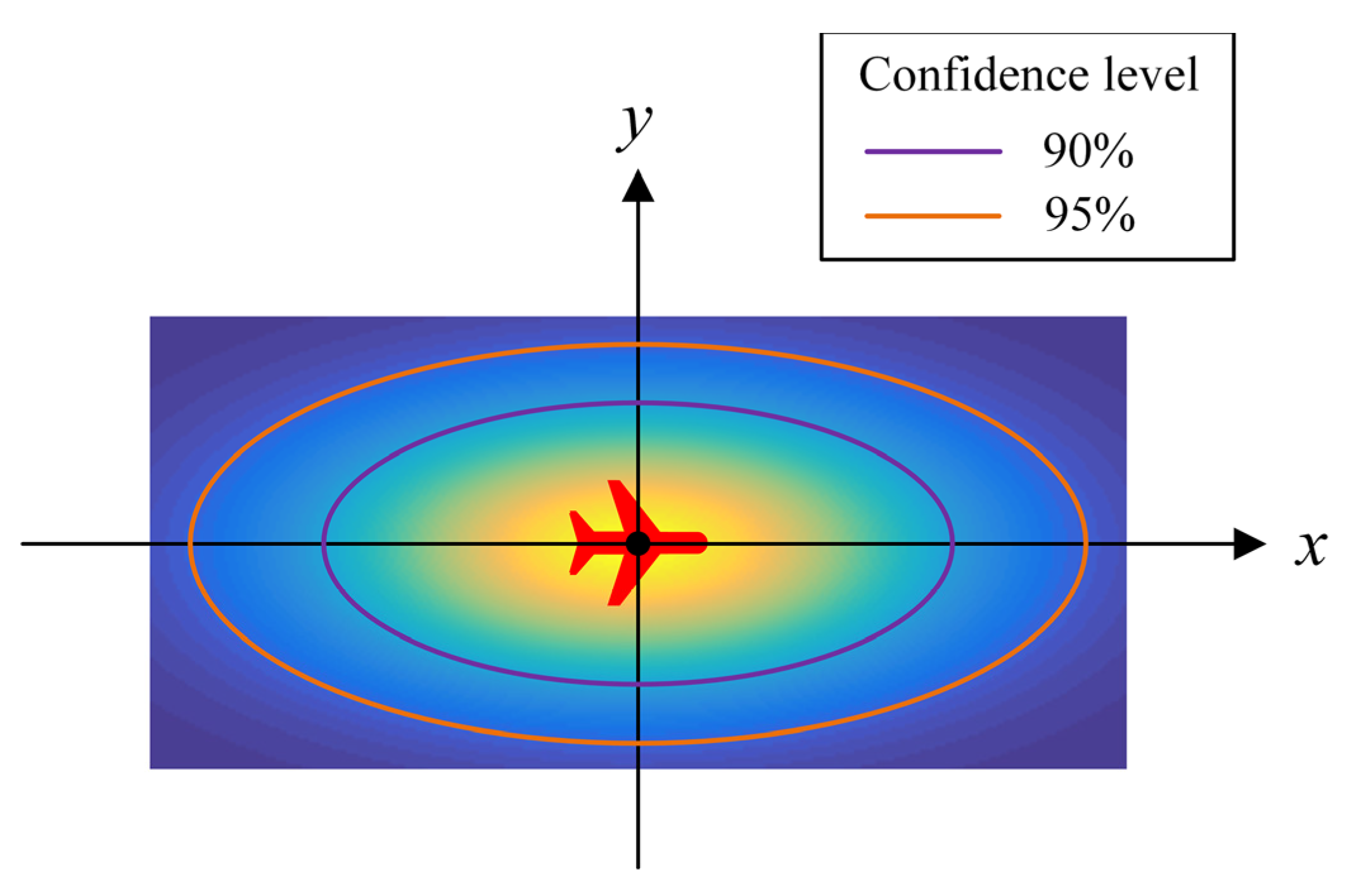
We rely on prediction of the aircraft’s future trajectory to detect conflicts and determine whether the conflict pair has been resolved. However, discrepancies between the actual and predicted trajectories can occur owing to navigation errors and errors in flight technique. In this work, we refer to the model proposed in [44] and consider the uncertainty in the real position of the aircraft on the horizontal plane. As shown in Figure 4, a plane rectangular coordinate system is established with the aircraft heading along the positive -axis, with the predicted aircraft position considered as the origin. Assuming that the real horizontal position of the aircraft is the point in the coordinate system, the two-dimensional random variable is subject to the following two-dimensional Gaussian distribution:
where and are the cross-track and along-track standard deviations, respectively. According to [44], is a constant, and is a linear function of time expressed as
where describes the growth of the along-track uncertainty with prediction time () in units of nautical miles per minute.
As shown in Figure 4, the confidence ellipse of the two-dimensional Gaussian distribution can be determined according to different confidence levels. Because ellipses are challenging to handle, it is assumed that the real horizontal position of the aircraft does not extend beyond the concentric tangent of the confidence ellipse. The aircraft can self-correct its course, so although the radius of this concentric tangent circle will increase with time, it will not exceed a specific value. This study assumes that the RNAV 1 navigation specification is used and considers this circle to have a maximum radius of 1 nm. The conflict detection mechanism proposed in this study is shown in Figure 5, where the green ellipse is the confidence ellipse, and are the major axis lengths of the two aircraft confidence ellipses, is the vertical separation of the two aircraft, and the confidence level is considered as 90%.
3.4. Resolution Scheme Based on ACKTR
The model-free DRL algorithms are used to solve the MDP. Such algorithms use the interaction with the environment to gain experience without a mathematical description of the environment, while relying only on experience (e.g., samples of trajectories) to learn an approximate representation of the optimal policy. The model-free DRL algorithms include optimal value, policy gradient, and actor–critic algorithms. This study uses the actor–critic algorithms because they combine the advantages of the other two algorithms, with high sample efficiency and powerful characterisation of the policy. The actor–critic algorithm uses a value network to approximate the value function and a policy network to approximate the optimal policy. In updating the parameters of neural networks, the natural gradient method is used to translate parameter updates into updates on model performance at each iteration. The Kullback–Leibler divergence constrains the distance between the old and new models. ACKTR is an actor–critic algorithm that uses the natural gradient method. ACKTR outperforms the trust region policy optimisation (TRPO), the advanced actor–critic (A2C), and Q-learning methods in terms of training efficiency on discrete control tasks [45].
3.4.1. Actor–Critic Using Kronecker-Factored Trust Region (ACKTR)
ACKTR [45] uses the Kronecker-factored approximate curvature (K-FAC) to approximate the Fisher information matrix to reduce the computational complexity of the natural gradient method. When using natural gradient descent, the parameter update method is given by
where is the function to be optimised, is the step size, and is the Fisher information matrix.
As the calculation of is very complex, it reduces the training speed. Therefore, to improve the efficiency of natural gradient descent, ACKTR uses K-FAC [46] to approximate the calculation of . We suppose that is the output distribution of a neural network, and is the log-likelihood output distribution. Furthermore, we suppose that is the weight matrix in the layer of the neural network, where and are the number of output and input neurons of the layer, respectively. The input activation vector to the layer is denoted as , and the preactivation vector for the next layer is denoted as . The weight gradient is expressed as . Let be a vectorized transformation that transforms a matrix into a one-dimensional vector. K-FAC approximates the block Fisher information matrix (), which corresponds to the layer as , which is expressed as
where and . Based on Equation (11) and two identities, and , we can deduce an efficient method to descend the natural gradient by approximate calculation as follows:
In this way, when updating the parameters of the layer of the neural network, it is converted from inverting a matrix with dimensions of to inversing two matrices with dimensions of and . The computational complexity is therefore reduced from to .
3.4.2. Training Process
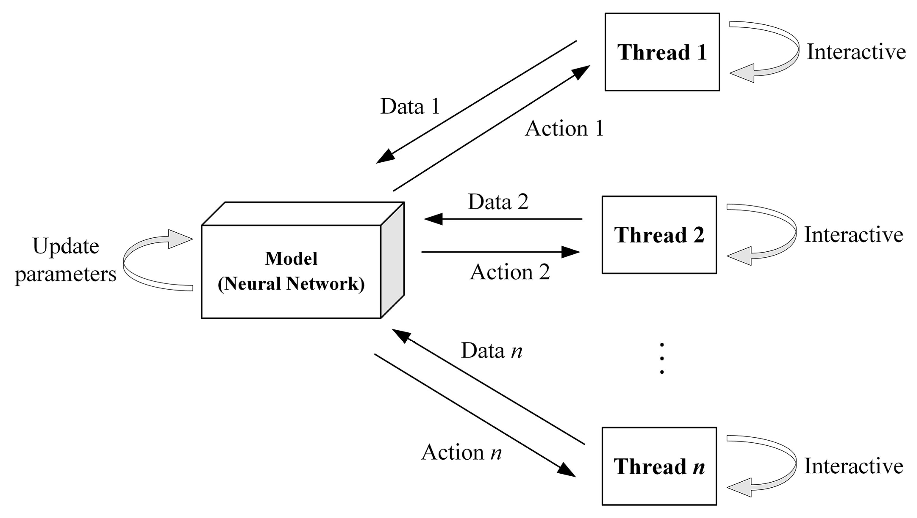
The multithreaded ACKTR is used to train the TCS agent. The agent in each thread interacts with its DRL environment, and the tasks of decision making and training are integrated into the model itself, as shown in Figure 6. in the figure indicates the total number of threads.
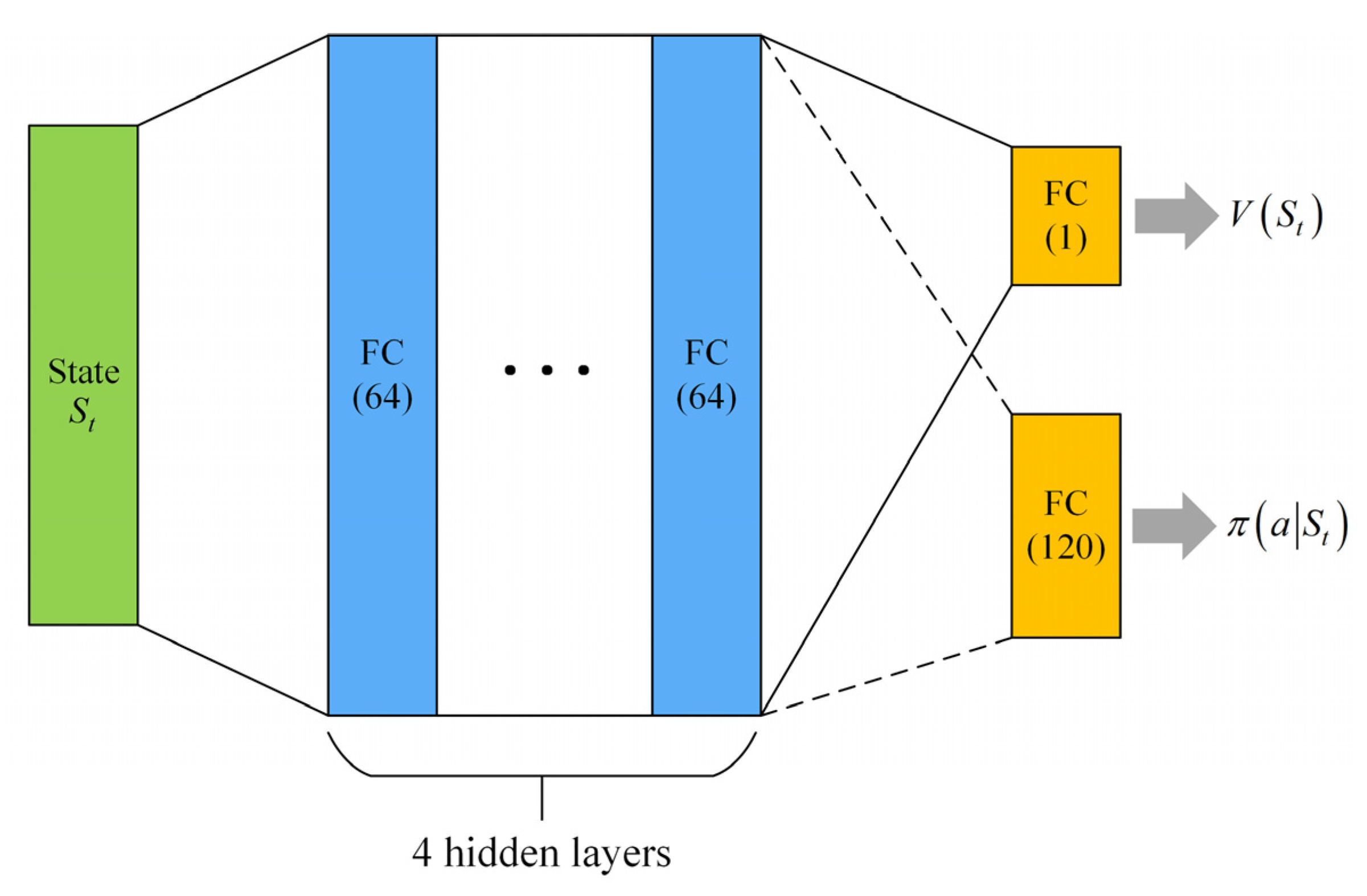
ACKTR uses the actor–critic architecture, which includes a policy network (, i.e., actor) and a value network (, i.e., critic). The output () of the policy network is a distribution; therefore, it is easy to define its Fisher information matrix. However, the output of the standard value network is scalar rather than a distribution; therefore, its Fisher information matrix cannot be defined. Therefore, ACKTR defines the output of the value network as a Gaussian distribution whose can be simply set to 1 in practice. We used the neural network architecture shown in Figure 7 to train the agent. The actor and the critic share a fully connected neural network with four hidden layers each of which connects a fully connected layer to output the value and policy. The numbers in parentheses in the figure represent the number of nodes in the neural network. ‘FC’ represents a fully connected layer.
The proposed neural network architecture can be regarded as a global neural network. Therefore, we can update the global network with only one loss function, that is, we can update the parameters of the critic and the actor simultaneously. Suppose that there are threads and that the agent in each thread interacts in steps with its environment in one multithreaded interaction; then, it collects the experience dataset (). Then, we have . The loss function is defined as Equation (13). Let and be the constant coefficients and be the action space.
where
To use the method of natural gradient descent to update the model, ACKRT defines the output of the global network as by assuming independence of the policy and the value distribution. Therefore, the parameter update formula of the global network is
where , and is the distribution of trajectories given by .
To adapt the TCS agent to various conflict scenarios, the agent should be provided with a large number of conflict scenario samples as the environment. The construction of the conflict scenario samples is described in Section 3.3.1, and the specific sample generation method is described in Section 3.1. Algorithm 1 shows the agent training process based on ACKTR. ACKTR sets in row 11 of the table to [47], where is the learning rate, is the trust region, and each block in the block diagonal matrix () corresponds to the Fisher information matrix () of each layer of the global network. To reduce instability in training for the conflict pair in the same conflict scenario sample, the agent’s first action is always for the aircraft specified in this conflict pair; if there is a second action, it is for the second aircraft.
Algorithm 1 shows the flow of the ACKTR algorithm used to train the TCS agent.
| Algorithm 1: ACKTR Algorithm for Training the TCS Agent | |
| 1: | Initialize the parameter of the global network. |
| 2: | Loop through iterations . |
| 3: | Each thread selects a conflict scenario sample randomly and initializes the state . |
| 4: | Loop through the steps . |
| 5: | Each thread generates its own trajectory with its policy . |
| 6: | Until the steps end. |
| 7: | Summarise the trajectory of each thread and calculate the loss function according to Equation (13). |
| 8: | For the layer of the global network, do: |
| 9: | , in the calculation of and , . |
| 10: | End for. |
| 11: | Use K-FAC to approximate the natural gradient to update the parameters of the global network: . |
| 12: | Until the iterations end. |
4. Results
4.1. Experimental Setup
- (1)
- Experiment and simulation environment
We developed a realistic airspace operating environment based on the ATOSS as the DRL environment, which interacts with the agent to generate the data required online. The ATOSS is also used for trajectory and airspace situation prediction, state transition, and conflict detection. Developed in our laboratory, ATOSS combines an airspace database with the Base of Aircraft Data (BADA) database for motion simulation of the engine to simulate the aircraft’s operational posture. It calculates the acceleration, speed, and rates of climb and descent of the aircraft based on parameters such as force and fuel consumption during each phase of the flight. It predicts the trajectory in conjunction with operational airspace rules.
The hardware environment for all experiments is an HP Z8 G4 workstation with an Intel Xeon(R) Gold 6242 CPU and 64 GB of RAM (manufacturer: Hewlett-Packard, Palo Alto, CA, USA). The software environment is IntelliJ PyCharm (version: Community Edition 2020.2.4 ×64), using Python to write the algorithms.
- (2)
- Conflict scenario samples
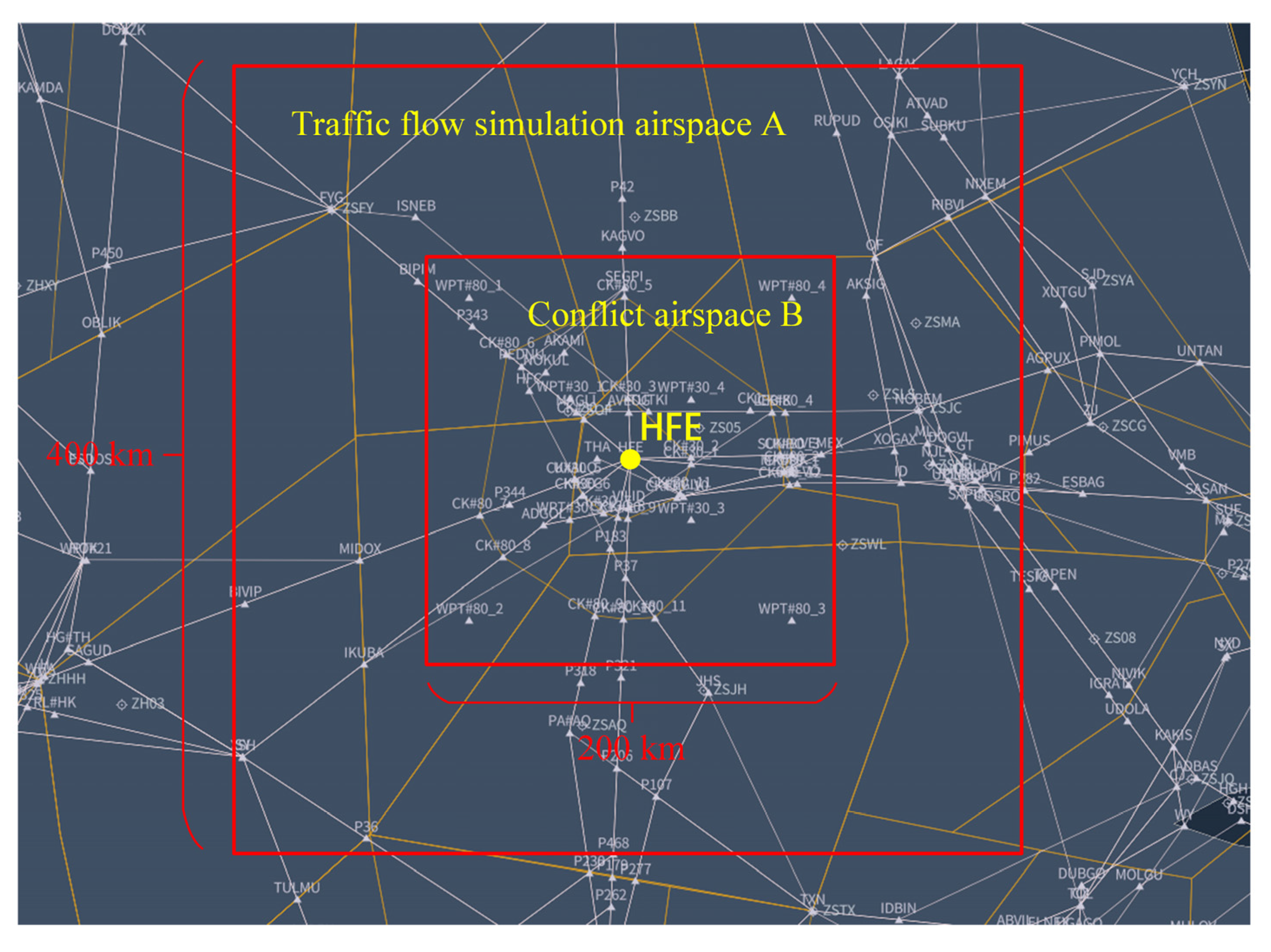
We used the ATOSS for airspace situational simulation to generate conflict scenario samples. Considering the HFE, the busiest waypoint in China in 2019 [48], as the central point, a cuboid airspace (i.e., airspace A) of 400 × 400 × 6 km was expanded as the airspace for the traffic flow simulation. Moreover, using the HFE as the central point, the cuboid airspace (i.e., airspace B) was expanded to 200 × 200 × 6 km; the conflict pairs in this airspace were recorded to generate conflict scenario samples, as shown in Figure 8.
The flight plans of the aircraft that flew through or landed in airspace A on 1 June 2018 were selected. To ensure sufficient time to resolve conflict pairs, plans that resulted in the aircraft taking less than 600 s to arrive at airspace A were removed. The remaining plans formed the simulation flight plan set to simulate traffic flow. The HFE is the route convergence point; therefore, its flow also reflects the flow in airspace A. The peak hourly flow at the HFE in 2019 was 106 flights/h [48], so 20–30 aircraft were allowed to arrive at airspace A within 10 min of one another to simulate the operation situation of airspace A at peak flow. The process of constructing the conflict scenario samples was as follows.
- Step 1: From the simulation flight plan set, 20–30 flights were randomly loaded, and the departure times of the flights were changed by adding random amounts to ensure that the flights arrived at airspace A within the 10 min window;
- Step 2: The detected conflict pairs in airspace B were recorded during the simulation. For each conflict pair, we determined whether the conflict scenario construction condition described in Section 3.3.1 was met. If so, a conflict scenario sample was generated for the period in which the conflict occurred;
- Step 3: Steps 1 and 2 were repeated until the number of conflict scenario samples satisfied the requirements.
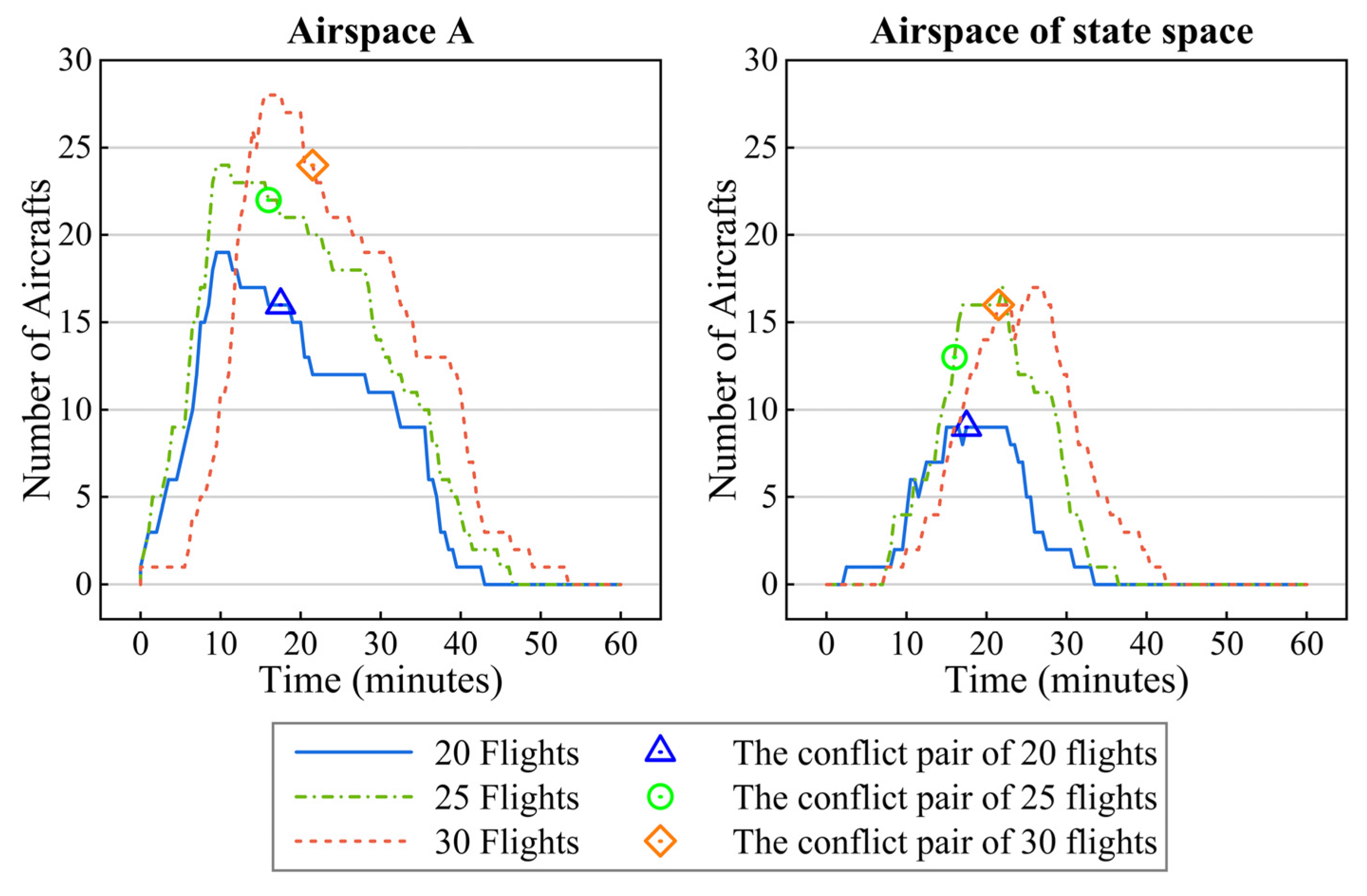
By performing the above steps, 6000 conflict scenario samples were obtained. Using the holdout method, 5000 samples were selected to constitute the training set, and the remaining 1000 samples constituted the testing set. Three conflict scenario samples were randomly selected and loaded with 20, 25, and 30 flights. The relationship between the number of aircraft and time in airspace A and the airspace of the state space (i.e., the km cuboid airspace centred at the conflict point) is shown in Figure 9. For each sample, the time when the first flight entered airspace A is 0. The results show that these samples provide reasonable airspace densities for airspace A. Figure 9 also shows that in each sample, the traffic density in the airspace of state space is near its peak at the time of the conflict pair; therefore, the samples are challenging to resolve.
- (3)
- Baseline algorithms
The baseline algorithms used in this work are Rainbow [49] and A2C [50]. Rainbow is an improved algorithm for deep Q networks and uses techniques such as double Q learning and prioritized replay buffer. It is an optimal-value algorithm with excellent performance. A2C has good performance among the actor–critic algorithms. The main difference between A2C and ACKTR is that A2C uses the gradient descent method when updating the parameters of neural networks, whereas ACKTR uses the natural gradient method. The test results of the untrained random agent are presented to observe the performance improvement of the agent after training.
4.2. Experimental Analysis
- (1)
- Determining the parameter combination
The DRL method mainly consists of the parameters in the reward function and the hyperparameters, and their settings affect the agent’s training. Six parameter combinations are set up to evaluate the impact of different combinations of hyperparameters and reward function parameters on training. Among the hyperparameters, the learning rate, which significantly impacts training, is chosen as the variable parameter. Experiments are conducted with different reward function parameters when the learning rate is and . We tested different values for , , and in Equations (4)–(6).
The hyperparameters of ACKTR are shown in Table 3. We used 32 threads for training following the multithreaded training mechanism described in Figure 6. In each thread, the agent interacts with the environment in two steps. The total training steps refer to the total number of steps in which the agents interact with the environment in all threads.
The six parameter combinations for ACKTR are shown in Table 4, demonstrating six combinations of the learning rate and reward function parameters at different values. We compared the TCS agent training results with six parameter combinations to select the best combination.
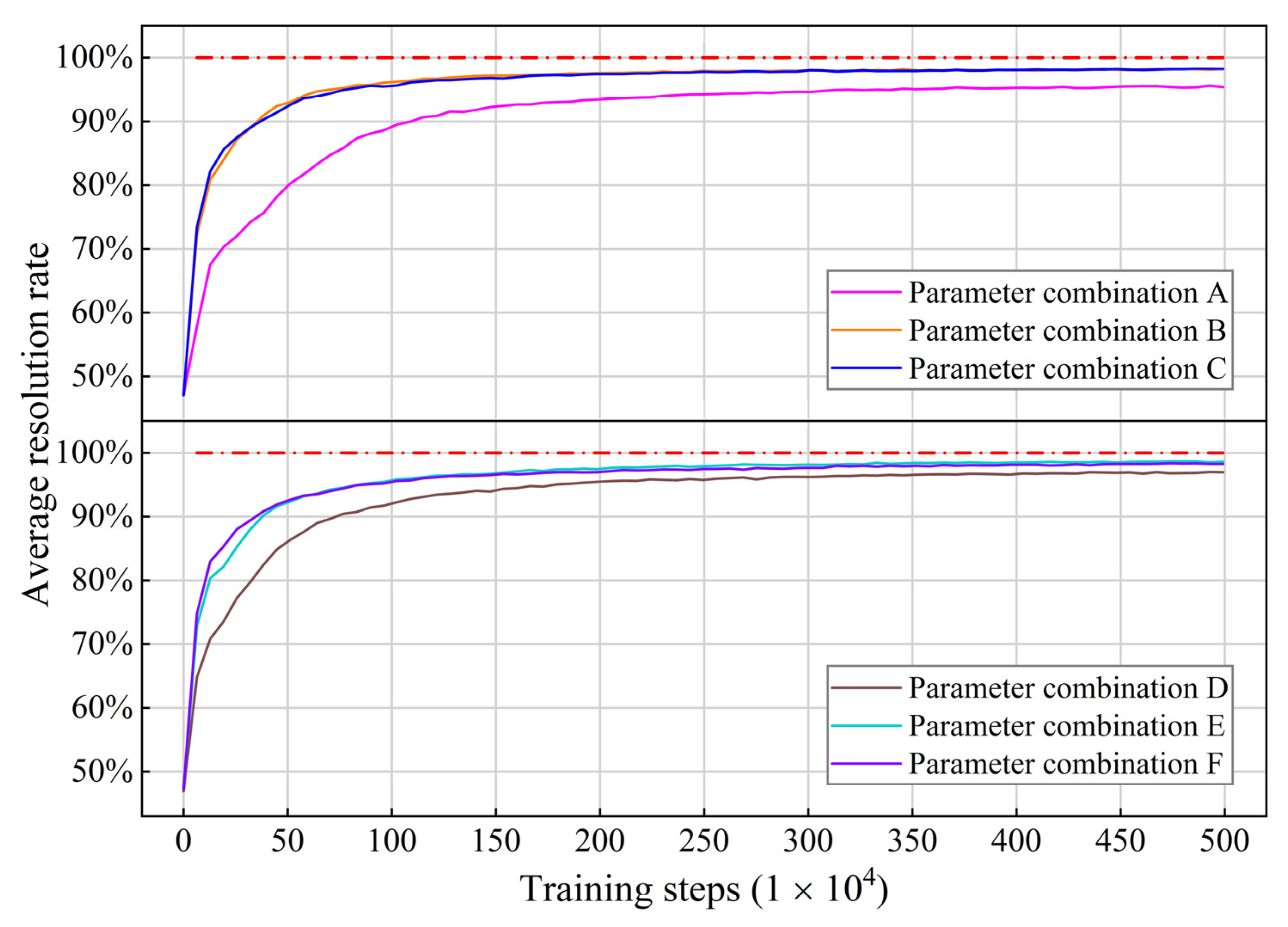
The same training set was used for the six parameter combinations. Because the reward function parameters differ, we used the average resolution rate during training to represent the effect. The average resolution rate is the percentage of conflict scenario samples resolved out of the samples selected in 1000 updates of the global network. The training process is shown in Figure 10. The high learning rate slightly improves the sample efficiency but has little impact on the convergence of the model. Irrespective of the sample efficiency or the post-convergence performance, combinations A and D were trained less effectively than other combinations. This may be because the reward values are too small, making the model insensitive to the feedback from the reward. In combinations B, C, E, and F, the observed training effects are similar, which also validates the robustness of the model.
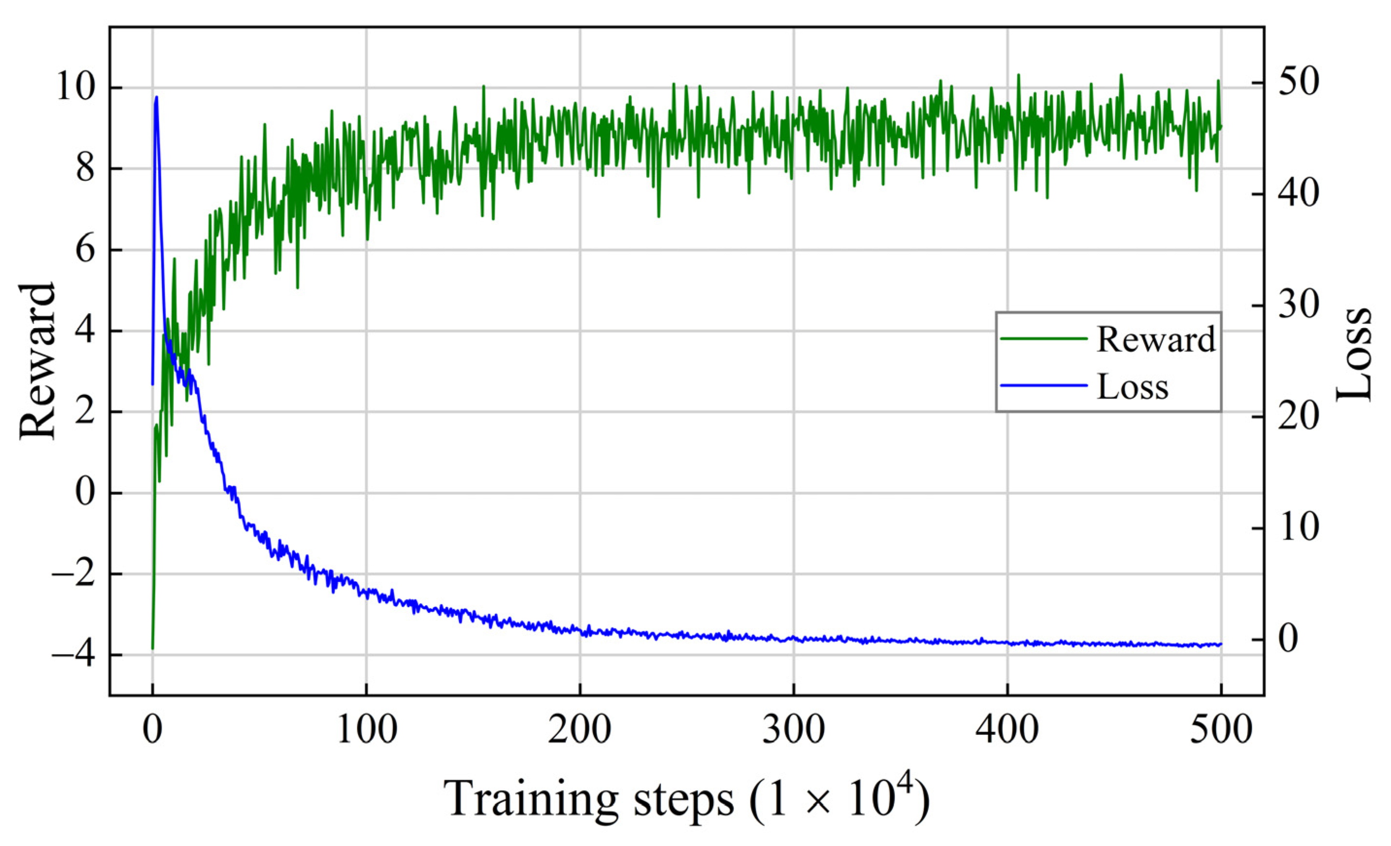
To describe the model’s performance after convergence, we present the training data after four million steps, as shown in Table 5. After convergence, combination C has the best average reward, and E has the highest average resolution rate. Our primary goal is to ensure that the conflict pairs can be resolved; therefore, we chose combination E as the final parameter of the model. The learning curve for combination E is shown in Figure 11. We averaged the rewards for every 100 updates of the global network to smooth the curve. As the reward values increased, the loss values decreased. Finally, they all converged. The model proved to be convergent.
- (2)
- Comparison with the baseline algorithms
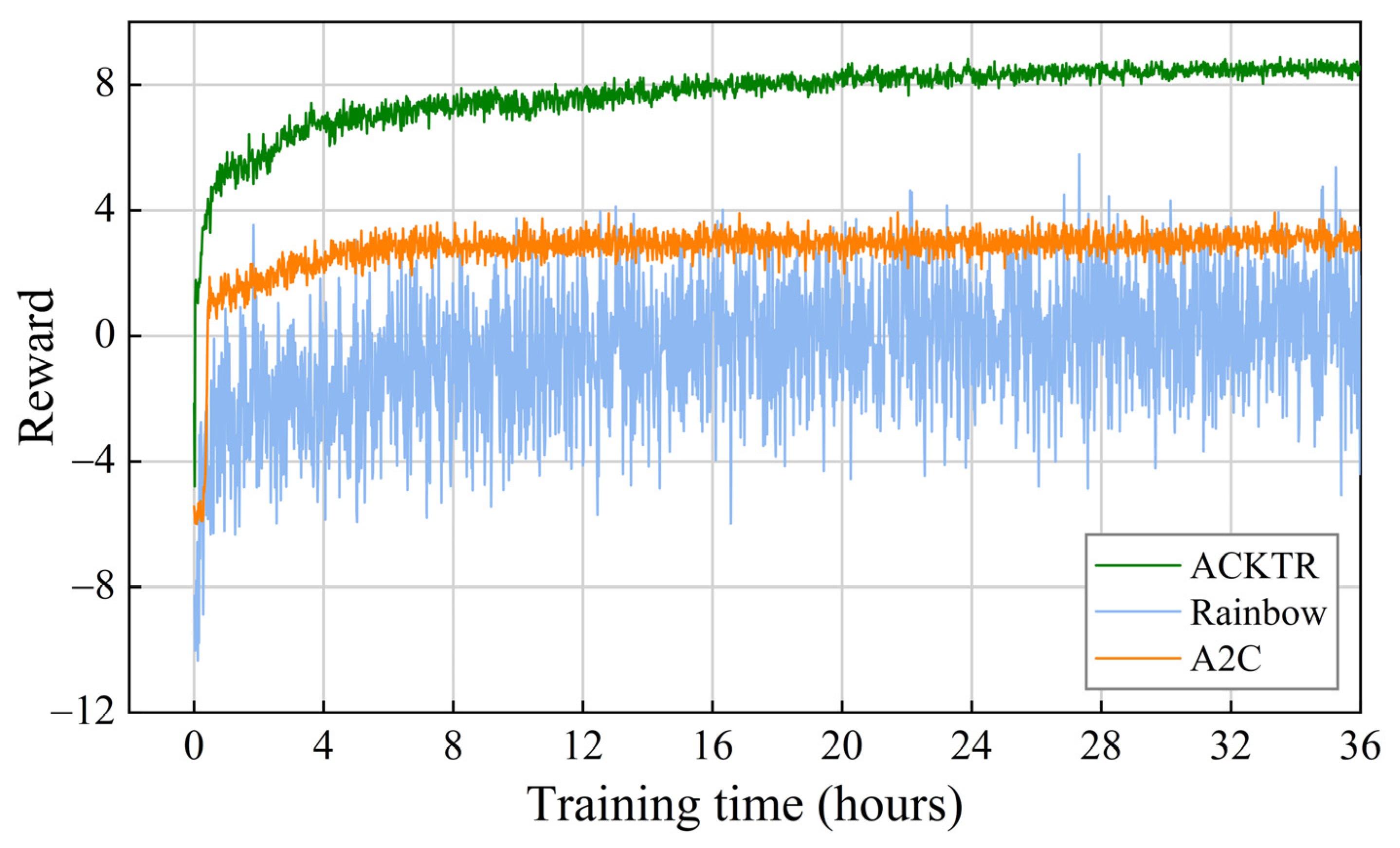
ACKTR, Rainbow, and A2C used the same reward function and dataset with the learning curves, as shown in Figure 12. We averaged the rewards for every 60 s of training. Table 6 presents the training data after 30 h of training time to observe the model performance after convergence. It can be seen that ACKTR outperformed the other two algorithms in terms of computational efficiency and post-convergence performance. Furthermore, as algorithms for training policy networks, ACKTR and A2C presented more minor training variances than those presented by Rainbow. The model performance of ACKTR continued to improve when A2C converged at approximately 4 h, demonstrating that the natural gradient method can make the model exceed the local optimum solution.
- (3)
- Model performance based on the testing set
A testing set containing 1000 test samples was used to test the model performance after convergence. In the first test of a test sample, the TCS agent gave one aircraft in the conflict pair the CR instruction; after that, if the conflict pair remained unresolved, the agent gave the other aircraft the CR instruction. The order of the CR instructions given to the conflicting aircraft was then reversed, and the test was performed again. The best of the two tests was then considered the final test result for that test sample.
Table 7 lists the test results for the different algorithms. The conflict resolution rate is the ratio of successfully resolved test samples to the total test samples. It is the most direct indicator of model performance. ACKTR has a conflict resolution rate of 87.1%, which is higher than that of the other two algorithms. Compared with the random agent, the ACKTR conflict resolution rate improved by 41.1%. When testing with ACKTR, the TCS was able to generate a CR scheme for each test sample and determined whether the scheme met CONDITION with the ATOSS in less than 4 s total time (1.13 s on average).
When using ACKTR for testing, the TCS can generate a CR scheme for each test sample in less than 4 s (1.13 s on average) and determine whether the scheme satisfies CONDITION through the ATOSS to verify the validity of the scheme. In contrast, CR methods using GA may take tens of seconds to find a suitable scheme [36].
Table 8 shows the distribution of the CR manoeuvres acting on the conflicting aircraft used by the TCS when tested with ACKTR. In most cases, the TCS used the altitude adjustment to resolve conflicts and rarely used speed and heading adjustments. This suggests that in the route intersection scenario used for the experiment (see Figure 8), it is easier to resolve conflicts by expanding the vertical separation of the aircraft than by expanding the horizontal separation. In addition, within the short, tactical resolution time horizon of 6 min, there may not be sufficient time to use speed and heading adjustments to expand the horizontal separation, so the agent did not tend to use speed and heading adjustment.
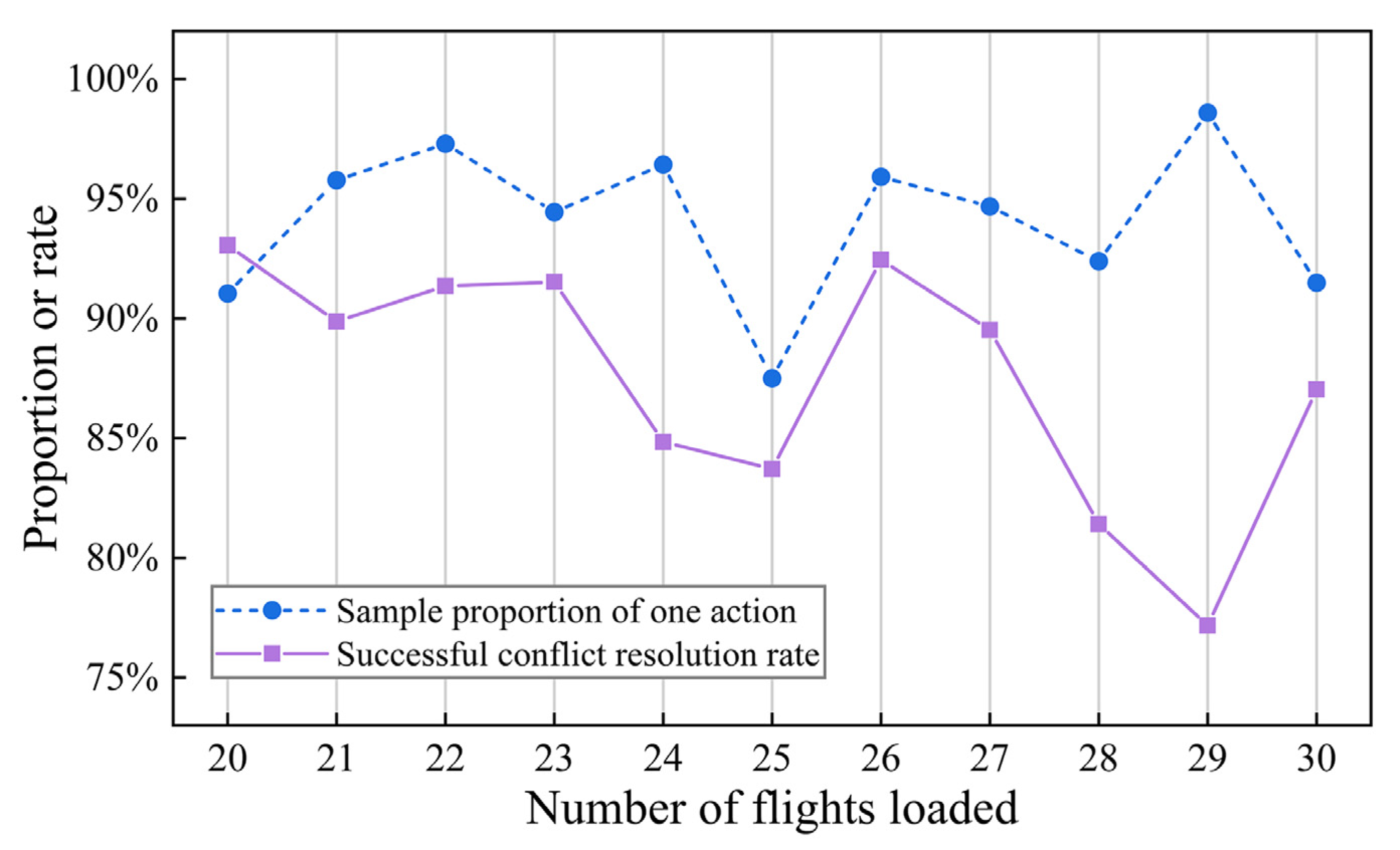
The TCS agent’s solution which uses one action to resolve the conflict pair is better than the solution which uses two actions. Among the 871 test samples that were successfully resolved using ACKTR, approximately 94.14% were resolved by a single action. Considering the samples resolved in the testing set, the relationship between the proportion of samples in which the agent performed one action and the number of flights loaded in the sample is shown in Figure 13. The figure also shows the relationship between the conflict resolution rate and the number of flights loaded in the sample. The number of flights loaded reflects the airspace density.
First, irrespective of the airspace density, the agent could adopt an action to resolve the conflict pair in more than 85% of the samples. In addition, there is no significant correlation between the two variables (see the blue dotted line in Figure 13), which implies that an increase in airspace density does not affect the quality of the solutions generated by the TCS in this airspace density range. Second, the conflict resolution rate shows a negative correlation with airspace density (see the purple solid line in Figure 13), indicating that the CR ability of the TCS decreases at high airspace density. This may be because the increase in airspace density leads to a reduction in the solution space, which increases the difficulty in resolving the conflict.
- (4)
- Performance of the model in higher-density airspace
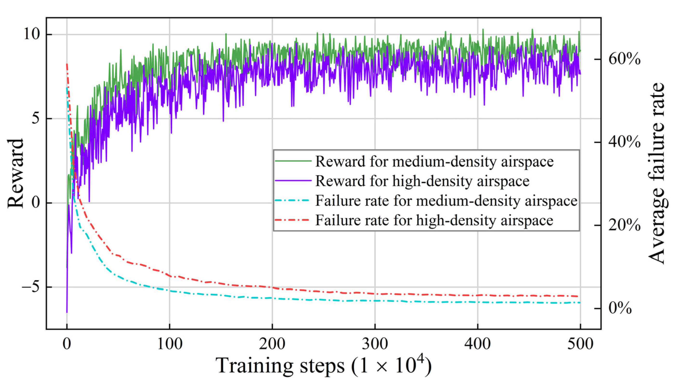
The situation in which 20–30 aircraft arrive at airspace A within 10 min is defined as medium-density airspace, and the situation in which 30–40 aircraft are loaded is defined as high-density airspace. The airspace density of the high-density airspace is 1.4 times that of the medium-density airspace. The training and testing process uses ACKTR. The training process is shown in Figure 14, where . The increase in airspace density leads to a slight decline in the training effect but does not lead to the collapse or divergence of the model, indicating that the model maintains good stability and convergence under the stress test.
The models were tested under high-density airspace using 1000 test samples. The conflict resolution rate for the model trained with ACKTR was 81.20%, whereas it was 39.00% for the random agent. With ACKTR, the conflict resolution rate in the high-density airspace was 5.9% lower than that in the medium-density airspace. With ACKTR, compared with the random agent, the conflict resolution rate of the trained agent was 42.2% higher, which approximated the performance improvement of the model under the medium-density airspace. This shows that although the increase in airspace density leads to a decline in the agent’s ability to resolve conflicts, the improvement of the agent’s ability to resolve conflicts using the DRL method is not inhibited.
4.3. Discussion
Tactical conflict resolution is an essential part of intelligent ATC. The critical problem in tactical conflict resolution is clarifying the framework and mechanism of CD&R and improving the model’s CR ability in various scenarios. This study proposes a receding horizontal control CD&R mechanism to assist ATCOs in CR. The TCS agent is trained using ACKTR, and experimental proofs are performed.
The CR model uses the same altitude, speed, and heading adjustments as the controllers. Using performance data from different aircraft types during the agent’s interaction with the environment can ensure that the model solutions fit the aircraft dynamic constraints. The uncertainty of the real horizontal position is inscribed with the two-dimensional Gaussian distribution during trajectory prediction, enhancing the feasibility of the CR schemes. Realistic airspace structure, flight plans, and airspace density are used in the training and testing sets to increase the model’s confidence. The conflict resolution rate did not reach 100%; however, a resolution rate of nearly 90% is acceptable for a tool that assists ATCOs in decision making. Nonetheless, it is necessary to improve the model’s performance model in future research.
We found that the conflict resolution rate of the testing set decreased as the airspace density increased. The underlying reason is that the airspace structure and traffic flow density determine the size of the available solution space. In practice, to ensure flight safety, airspace density is usually restricted by holding aircraft or controlling traffic flow.
The work in this study enriches the research methods in tactical conflict resolution. It enhances the intelligence of CR models, which can be used as a reference for intelligent ATC auxiliary decision-making systems in the future.
5. Conclusions
This study proposes a receding horizontal control CD&R mechanism to handle continuous traffic flow with CD&R on the continuous time horizon. Considering ATC regulations, uncertainty in real environments. and actual airspace structures, the TCS agent is trained using ACKTR to assist ATCOs in resolving conflict pairs. We incorporated the trajectory prediction error into the training and testing sets to ensure the robustness of the TCS in uncertain environments. The results show that using ACKTR to train the agent can resolve most conflict pairs with only one CR instruction in the actual airspace structure and density. The training is completed within 38 h, which is not much time for the complex CR task. The final conflict resolution rate exceeded 87%, and the TCS could find the CR scheme within an average of 1.13 s. Even when the airspace density was increased by a factor of 1.4, the conflict resolution rate exceeded 80%. The scope for future work can be described according to the following aspects. (1) The controllers’ experience can be extracted from historical data to make the generated CR strategy conform to the habits of ATCOs. (2) Adjustments to neighbouring aircraft can be added to increase the solution space during conflict resolution.
Author Contributions
Conceptualization, D.S.; methodology, C.M.; software, C.M.; validation, C.M. and C.W.; formal analysis, D.S.; investigation, D.S.; resources, D.S.; data curation, C.M.; writing—original draft preparation, C.M.; writing—review and editing, C.M.; visualization, C.M.; supervision, D.S., C.M. and C.W.; project administration, D.S.; funding acquisition, D.S. All authors have read and agreed to the published version of the manuscript.
Funding
The work was funded by the Safety Ability Project of the Civil Aviation Administration of China (No.: TM 2018-5-1/2). The project was funded by the Civil Aviation Administration of China (CAAC).
Institutional Review Board Statement
Not applicable.
Informed Consent Statement
Not applicable.
Data Availability Statement
Restrictions apply to the availability of these data. Data were obtained from the Air Traffic Management Bureau (ATMB) of the Civil Aviation Administration of China (CAAC) and are available from the authors with the permission of the ATMB of the CAAC.
Acknowledgments
This work was jointly completed by the project team members of the Intelligent Air Traffic Control Laboratory of Nanjing University of Aeronautics and Astronautics. The completion of this article would have been impossible without the efforts of each member. I would like to thank the associated teachers for their guidance and suggestions.
Conflicts of Interest
The authors declare that they have no known competing financial interests or personal relationships that may affect the work described in this paper.
References
- Walker, C. All-Causes Delay and Cancellations to Air Transport in Europe: Annual Report for 2019; Eurocontrol: Brussels, Belgium, 2019; Available online: https://www.eurocontrol.int/publication/all-causes-delay-and-cancellations-air-transport-europe-2019 (accessed on 23 October 2022).
- Federal Aviation Administration. Air Traffic by the Numbers [Internet]; Federal Aviation Administration: Washington, DC, USA, 2022. Available online: https://www.faa.gov/air_traffic/by_the_numbers/media/Air_Traffic_by_the_Numbers_2022.pdf (accessed on 23 October 2022).
- Civil Aviation Administration of China. Statistical Bulletin of Civil Aviation Industry Development in 2020 [Internet]; Civil Aviation Administration of China: Beijing, China, 2022. Available online: http://www.caac.gov.cn/en/HYYJ/NDBG/202202/P020220222322799646163.pdf (accessed on 23 October 2022).
- Isaacson, D.R.; Erzberger, H. Design of a conflict detection algorithm for the Center/TRACON automation system. In Proceedings of the 16th DASC, AIAA/IEEE Digital Avionics Systems Conference: Reflections to the Future, Irvine, CA, USA, 30 October 1997. [Google Scholar]
- Brudnicki, D.J.; Lindsay, K.S.; McFarland, A.L. Assessment of field trials, algorithmic performance, and benefits of the user request evaluation tool (uret) conflict probe. In Proceedings of the 16th DASC, AIAA/IEEE Digital Avionics Systems Conference: Reflections to the Future, Irvine, CA, USA, 30 October 1997. [Google Scholar]
- Torres, S.; Dehn, J.; McKay, E.; Paglione, M.M.; Schnitzer, B.S. En-Route Automation Modernization (ERAM) trajectory model evolution to support trajectory-based operations (TBO). In Proceedings of the Digital Avionics Systems Conference. IEEE/AIAA. 34th 2015. (DASC 2015) (3 VOLS), Prague, Czech Republic, 13–17 September 2015; p. 1A6-1. [Google Scholar]
- Brooker, P. Airborne Separation Assurance Systems: Towards a work programme to prove safety. Saf. Sci. 2004, 42, 723–754. [Google Scholar] [CrossRef] [Green Version]
- Kuchar, J.E.; Drumm, A.C. The traffic alert and collision avoidance system. Linc. Lab. J. 2007, 16, 277. [Google Scholar]
- Kochenderfer Mykel, J.; Jessica EHolland James, P. Chryssanthacopoulos: ‘Next-Generation Airborne Collision Avoidance System’; Massachusetts Institute of Technology-Lincoln Laboratory: Lexington, MA, USA, 2012. [Google Scholar]
- Owen, M.P.; Panken, A.; Moss, R.; Alvarez, L.; Leeper, C. ‘ACAS Xu: Integrated collision avoidance and detect and avoid capability for UAS’. In Proceedings of the AIAA 2019 38th Digital Avionics System Conference (DASC), San Diego, CA, USA, 8–12 September 2019; pp. 1–10. [Google Scholar]
- Eurocontrol. European ATM Master Plan [Internet]; Eurocontrol: Brussels, Belgium, 2020; Available online: https://www.sesarju.eu/sites/default/files/documents/reports/European%20ATM%20Master%20Plan%202020%20Exec%20View.pdf (accessed on 23 October 2022).
- International Civil Aviation Organization. Doc 9854, Global Air Traffic Management Operational Concept; International Civil Aviation Organization: Montreal, QC, Canada, 2005. [Google Scholar]
- Kuchar, J.K.; Yang, L.C. A review of conflict detection and resolution modeling methods. IEEE Trans. Intell. Transp. Syst. 2000, 1, 179–189. [Google Scholar] [CrossRef] [Green Version]
- Ribeiro, M.; Ellerbroek, J.; Hoekstra, J. Review of conflict resolution methods for manned and unmanned aviation. Aerospace 2020, 7, 79. [Google Scholar] [CrossRef]
- Tang, J. Conflict detection and resolution for civil aviation: A literature survey. IEEE Aerosp. Electron. Syst. Mag. 2019, 34, 20–35. [Google Scholar] [CrossRef]
- Soler, M.; Kamgarpour, M.; Lloret, J.; Lygeros, J. A hybrid optimal control approach to fuel-efficient aircraft conflict avoidance. IEEE Trans. Intell. Transp. Syst. 2016, 17, 1826–1838. [Google Scholar] [CrossRef]
- Matsuno, Y.; Tsuchiya, T.; Matayoshi, N. Near-optimal control for aircraft conflict resolution in the presence of uncertainty. J. Guid. Control Dyn. 2016, 39, 326–338. [Google Scholar] [CrossRef]
- Liu, W.; Liang, X.; Ma, Y.; Liu, W. Aircraft trajectory optimisation for collision avoidance using stochastic optimal control. Asian J. Control 2019, 21, 2308–2320. [Google Scholar] [CrossRef]
- Cafieri, S.; Omheni, R. Mixed-integer nonlinear programming for aircraft conflict avoidance by sequentially applying velocity and heading angle changes. Eur. J. Oper. Res. 2017, 260, 283–290. [Google Scholar] [CrossRef] [Green Version]
- Cai, J.; Zhang, N. Mixed integer nonlinear programming for aircraft conflict avoidance by applying velocity and altitude changes. Arab. J. Sci. Eng. 2019, 44, 8893–8903. [Google Scholar] [CrossRef]
- Alonso-Ayuso, A.; Escudero, L.F.; Martín-Campo, F.J. Multiobjective optimisation for aircraft conflict resolution. A metaheuristic approach. Eur. J. Oper. Res. 2016, 248, 691–702. [Google Scholar] [CrossRef]
- Omer, J. A space-discretized mixed-integer linear model for air-conflict resolution with speed and heading maneuvers. Comput. Oper. Res. 2015, 58, 75–86. [Google Scholar] [CrossRef] [Green Version]
- Cecen, R.K.; Cetek, C. Conflict-free en-route operations with horizontal resolution manoeuvers using a heuristic algorithm. Aeronaut J. 2020, 124, 767–785. [Google Scholar] [CrossRef]
- Hong, Y.; Choi, B.; Oh, G.; Lee, K.; Kim, Y. Nonlinear conflict resolution and flow management using particle swarm optimisation. IEEE Trans. Intell. Transp. Syst. 2017, 18, 3378–3387. [Google Scholar] [CrossRef]
- Cecen, R.K.; Saraç, T.; Cetek, C. Meta-heuristic algorithm for aircraft pre-tactical conflict resolution with altitude and heading angle change maneuvers. Top 2021, 29, 629–647. [Google Scholar] [CrossRef]
- Durand, N.; Alliot, J.; Noailles, J. Automatic aircraft conflict resolution using genetic algorithms. In Proceedings of the SAC ’96-ACM Symposium on Applied Computing, Philadelphia, PA, USA, 17–19 February 1996; pp. 289–298. [Google Scholar]
- Ma, Y.; Ni, Y.; Liu, P. Aircraft conflict resolution method based on ADS-B and genetic algorithm. In Proceedings of the 2013 Sixth International Symposium on Computational Intelligence and Design, Washington, DC, USA, 28–29 October 2013. [Google Scholar]
- Emami, H.; Derakhshan, F. Multi-agent based solution for free flight conflict detection and resolution using particle swarm optimisation algorithm. UPB Sci. Bull. Ser. C Electr. Eng. 2014, 76, 49–64. [Google Scholar]
- Sui, D.; Zhang, K. A tactical conflict detection and resolution method for en route conflicts in trajectory-based operations. J. Adv. Transp. 2022, 2022, 1–16. [Google Scholar] [CrossRef]
- Durand, N.; Guleria, Y.; Tran, P.; Pham, D.T.; Alam, S. A machine learning framework for predicting ATC conflict resolution strategies for conformal automation. In Proceedings of the 11th SESAR Innovation Days, Virtual, 7–9 December 2021. [Google Scholar]
- Kim, K.; Deshmukh, R.; Hwang, I. Development of data-driven conflict resolution generator for en-route airspace. Aerosp. Sci. Technol. 2021, 114, 106744. [Google Scholar] [CrossRef]
- Van Rooijen, S.J.; Ellerbroek, J.; Borst, C.; van Kampen, E. Toward individual-sensitive automation for air traffic control using convolutional neural networks. J. Air. Transp. 2020, 28, 105–113. [Google Scholar] [CrossRef]
- Wang, Z.; Li, H.; Wang, J.; Shen, F. Deep reinforcement learning based conflict detection and resolution in air traffic control. IET Intell. Transp. Syst. 2019, 13, 1041–1047. [Google Scholar] [CrossRef]
- Pham, D.T.; Tran, N.P.; Goh, S.K.; Alam, S.; Duong, V. Reinforcement learning for two-aircraft conflict resolution in the presence of uncertainty. In Proceedings of the 2019 IEEE-RIVF International Conference on Computing and Communication Technologies (RIVF), Danang, Vietnam, 20–22 March 2019; pp. 1–6. [Google Scholar]
- Tran, P.N.; Pham, D.T.; Goh, S.K.; Alam, S.; Duong, V. An interactive conflict solver for learning air traffic conflict resolutions. J. Aerosp. Inf. Syst. 2020, 17, 271–277. [Google Scholar] [CrossRef]
- Sui, D.; Xu, W.; Zhang, K. Study on the resolution of multi-aircraft flight conflicts based on an IDQN. Chin. J. Aeronaut. 2022, 35, 195–213. [Google Scholar] [CrossRef]
- Dalmau-Codina, R.; Allard, E. Air traffic control using message passing neural networks and multi-agent reinforcement learning. In Proceedings of the 10th SESAR Innovation Days (SID), Virtual, 7–10 December 2020. [Google Scholar]
- Brittain, M.; Wei, P. One to any: Distributed conflict resolution with deep multi-agent reinforcement learning and long short-term memory. In Proceedings of the AIAA Scitech 2021, Virtual, 11–15 & 19–21 January 2021; p. 1952. [Google Scholar]
- Brittain, M.; Wei, P.; Brittain, M. Scalable autonomous separation assurance with heterogeneous multi-agent reinforcement learning. IEEE Trans. Autom. Sci. Eng. 2022, 19, 2837–2848. [Google Scholar] [CrossRef]
- Isufaj, R.; Aranega Sebastia, D.; Angel Piera, M. Toward conflict resolution with deep multi-agent reinforcement learning. J. Air Transp. 2022, 30, 71–80. [Google Scholar] [CrossRef]
- Ribeiro, M.; Ellerbroek, J.; Hoekstra, J. Determining optimal conflict avoidance manoeuvres at high densities with reinforcement learning. In Proceedings of the Tenth SESAR Innovation Days Virtual Conference, Virtual, 7–10 December 2020; pp. 7–10. [Google Scholar]
- Ribeiro, M.; Ellerbroek, J.; Hoekstra, J. Improvement of conflict detection and resolution at high densities through reinforcement learning. In Proceedings of the ICRAT 2020: International Conference on Research in Air Transportation, Tampa, FL, USA, 23–26 June 2020. [Google Scholar]
- International Civil Aviation Organization. Doc 4444, Procedures for Air Navigation Services—Air Traffic Management; International Civil Aviation Organization: Montreal, QC, Canada, 2016. [Google Scholar]
- Lauderdale, T. Probabilistic conflict detection for robust detection and resolution. In Proceedings of the 12th AIAA Aviation Technology, Integration, and Operations (ATIO) Conference and 2012 14th AIAA/ISSMO Multidisciplinary Analysis and Optimisation Conference, Indianpolis, IN, USA, 17–19 September 2012; p. 5643. [Google Scholar]
- Wu, Y.; Mansimov, E.; Grosse, R.B.; Liao, S.; Ba, J. Scalable trust-region method for deep reinforcement learning using kronecker-factored approximation. Adv. Neural Inf. Process. Syst. 2017, 30, 1–14. [Google Scholar]
- Martens, J.; Grosse, R. Optimizing neural networks with kronecker-factored approximate curvature. In Proceedings of the 32nd International Conference on Machine Learning, Lille, France, 7–9 July 2015; Bach, F., Blei, D., Eds.; PMLR: Lille, France, 2015; pp. 2408–2417. [Google Scholar]
- Ba, J.; Grosse, R.; Martens, J. Distributed second-order optimisation using Kronecker-Factored approximations. In Proceedings of the 5th International Conference on Learning Representations, Toulon, France, 24–26 April 2017. [Google Scholar]
- Civil Aviation Administration of China. Report of Civil Aviation Airspace Development in China 2019; Civil Aviation Administration of China: Beijing, China, 2020. [Google Scholar]
- Hessel, M.; Modayil, J.; Van Hasselt, H.; Schaul, T.; Ostrovski, G.; Dabney, W.; Horgan, D.; Piot, B.; Azar, M.; Silver, D. Rainbow: Combining improvements in deep reinforcement learning. In Proceedings of the Thirty-Second AAAI Conference on Artificial Intelligence, New Orleans, LA, USA, 2–7 February 2018; AAAI: Palo Alto, CA, USA, 2018. [Google Scholar]
- OpenAI, Inc., San Francisco. Openai.com/blog/baselines-acktr-a2c. Available online: https://openai.com/blog/baselines-acktr-a2c/ (accessed on 23 October 2022).
Figure 1.
CD&R framework diagram.

Figure 2.
CD&R mechanism in continuous time.

Figure 3.
Schematic diagram of a conflict scenario.

Figure 4.
Real horizontal position obeys a two-dimensional Gaussian distribution.

Figure 5.
Conflict detection under uncertain conditions.

Figure 6.
Multithreaded training mechanism.

Figure 7.
Neural network architecture for agent training.

Figure 8.
Traffic simulation and conflict airspace.

Figure 9.
Number of aircraft in the two airspaces changing with time.

Figure 10.
Resolution rate changes with training steps under different parameter combinations.

Figure 11.
Learning curves of parameter combination E.

Figure 12.
Training speed of ACKTR, Rainbow, and A2C on the same training set.

Figure 13.
Performance of the TCS under different numbers of flights.

Figure 14.
Training data of high-density and medium-density airspace (using AKCTR).


Table 1.
Features of conflict resolution methods.
| Category | Scholars | Specific Methods | Assisting ATCOs | CR Manoeuvres | Uncertainty | Complete and Detailed CD&R | Solution Time |
|---|---|---|---|---|---|---|---|
| Optimal control | Soler [16] | Hybrid optimal control | ✕ | 2D | ✕ | ✕ | 474 s |
| Matsuno [17] | Stochastic near-optimal control | ✕ | 2D | ◯ | ✕ | 38–231 s | |
| Liu [18] | Stochastic optimal control | ✕ | 2D | ◯ | ✕ | 115.3 s | |
| Mathematical programming | Cafieri [19] | MINLP | ◯ | 2D | ✕ | ✕ | 0.04–2561.98 s |
| Cai [20] | MINLP | ◯ | 3D | ✕ | ✕ | 3.131–75.102 s | |
| Alonso-Ayuso [21] | MINLP | ◯ | 3D | ✕ | ✕ | 0.32–24.00 s | |
| Omer [22] | MILP | ◯ | 2D | ✕ | ✕ | Within 8.3 s | |
| Cecen [23] | MILP | ✕ | 2D | ✕ | ✕ | 3.8–17 s | |
| Hong [24] | Nonlinear programming | ◯ | 2D | ✕ | ✕ | Within 11 s | |
| Cecen [25] | Two-step optimisation | ✕ | 3D | ✕ | ✕ | Within 240 s | |
| Swarm intelligence optimisation or search methods | Durand [26] | GA | ◯ | 2D | ◯ | ✕ | - |
| Ma [27] | GA | ✕ | 2D | ✕ | ✕ | - | |
| Emami [28] | PSO | ✕ | 3D | ✕ | ✕ | - | |
| Sui [29] | MCTS | ◯ | 3D | ✕ | ◯ | Average 12.44 s | |
| Supervised learning | Durand [30] | Random forests | ◯ | 2D | ✕ | ✕ | - |
| Kim [31] | Hierarchical classification | ◯ | 3D | ✕ | ✕ | Within 0.1 s | |
| Van Rooijen [32] | Convolutional neural networks | ◯ | 2D | ✕ | ✕ | - | |
| DRL | Wang [33] | KCAC | ◯ | 2D | ✕ | ✕ | 0.762 s |
| Pham [34] | DDPG | ◯ | 2D | ◯ | ✕ | - | |
| Tran [35] | DDPG | ◯ | 2D | ✕ | ✕ | - | |
| Sui [36] | IDQN | ◯ | 3D | ✕ | ✕ | Average 0.011 s | |
| Dalmau-Codina [37] | MARL | ◯ | 2D | ✕ | ✕ | - | |
| Brittain [38] | PPO | ✕ | 2D | ✕ | ◯ | - | |
| Brittain [39] | PPO | ✕ | 2D | ✕ | ◯ | - | |
| Isufaj [40] | MADDPG | ✕ | 2D | ✕ | ✕ | - | |
| Ribeiro [41] | DDPG and MVP | ✕ | 3D | ✕ | ✕ | - | |
| Ribeiro [42] | DDPG and MVP | ✕ | 2D | ✕ | ✕ | - |
Note: ◯ denotes that the conditions are met; ✕ denotes that the conditions are not met; ‘-’ denotes not described in the literature.
Table 2.
The CR instructions (i.e., the action space).
| CR Manoeuvre | Resolution Action | Adjustment Value | Waiting Time |
|---|---|---|---|
| Altitude adjustment | Climbing or descending/m | 300, 600, 900 | 20x s |
| Speed adjustment | Acceleration or deceleration/kt | 10, 20 | |
| Heading adjustment | Right or left offset/nm | 6 |
Table 3.
Hyperparameter values of ACKTR.
| Hyperparameter | Parameter Value | Hyperparameter | Parameter Value |
|---|---|---|---|
| Total training steps | 5,000,000 | 0.0005 | |
| Discount factor | 0.99 | 0.6 | |
| Number of threads | 32 | 0.3 | |
| Interaction steps per thread | 2 | Learning rate |
Table 4.
Different parameter combinations for ACKTR.
| Combination Name | Learning Rate | |||
|---|---|---|---|---|
| Combination A | 5.0 × 10⁻⁴ | 5 | 0.2 | |
| Combination B | 5.0 × 10⁻⁴ | 10 | 0.6 | |
| Combination C | 5.0 × 10⁻⁴ | 20 | 1 | |
| Combination D | 1.0 × 10⁻³ | 5 | 0.2 | |
| Combination E | 1.0 × 10⁻³ | 10 | 0.6 | |
| Combination F | 1.0 × 10⁻³ | 20 | 1 |
Table 5.
Training data of six parameter combinations.
| Combination Name | Average Reward after Four Million Steps Divided by Optimal Reward | Average Resolution Rate after Four Million Steps |
|---|---|---|
| A | 72.19% | 95.39% |
| B | 84.31% | 98.14% |
| C | 87.13% | 98.15% |
| D | 73.16% | 96.86% |
| E | 85.16% | 98.58% |
| F | 86.20% | 98.21% |
Table 6.
Training data of different algorithms.
| Algorithm | Average Reward after 30 h | Average Resolution Rate after 30 h |
|---|---|---|
| ACKTR | 9.03 | 98.58% |
| A2C | 3.07 | 79.32% |
| Rainbow | 0.16 | 67.82% |
Table 7.
Performance of different algorithms on 1000 test samples.
| Algorithm | Conflict Resolution Rate | Average Reward | Median Reward |
|---|---|---|---|
| ACKTR | 87.10% | 6.54 | 10.60 |
| Rainbow | 75.30% | 2.73 | 10.60 |
| A2C | 83.60% | 5.29 | 10.60 |
| Random agent | 46.00% |
Table 8.
Distribution of the CR manoeuvres performed by the TCS.
| CR Manoeuvre | Frequency | CR Manoeuvre | Frequency |
|---|---|---|---|
| Climbing (300 m) | 188 | Acceleration (10 kt) | 0 |
| Climbing (600 m) | 116 | Acceleration (20 kt) | 0 |
| Climbing (900 m) | 11 | Deceleration (10 kt) | 0 |
| Descending (300 m) | 253 | Deceleration (20 kt) | 3 |
| Descending (600 m) | 486 | Right offset (6 nm) | 6 |
| Descending (900 m) | 117 | Left offset (6 nm) | 0 |
Disclaimer/Publisher’s Note: The statements, opinions and data contained in all publications are solely those of the individual author(s) and contributor(s) and not of MDPI and/or the editor(s). MDPI and/or the editor(s) disclaim responsibility for any injury to people or property resulting from any ideas, methods, instructions or products referred to in the content. |
© 2023 by the authors. Licensee MDPI, Basel, Switzerland. This article is an open access article distributed under the terms and conditions of the Creative Commons Attribution (CC BY) license (https://creativecommons.org/licenses/by/4.0/).
Share and Cite
MDPI and ACS Style
Sui, D.; Ma, C.; Wei, C. Tactical Conflict Solver Assisting Air Traffic Controllers Using Deep Reinforcement Learning. Aerospace 2023, 10, 182. https://doi.org/10.3390/aerospace10020182
AMA Style
Sui D, Ma C, Wei C. Tactical Conflict Solver Assisting Air Traffic Controllers Using Deep Reinforcement Learning. Aerospace. 2023; 10(2):182. https://doi.org/10.3390/aerospace10020182
Chicago/Turabian StyleSui, Dong, Chenyu Ma, and Chunjie Wei. 2023. "Tactical Conflict Solver Assisting Air Traffic Controllers Using Deep Reinforcement Learning" Aerospace 10, no. 2: 182. https://doi.org/10.3390/aerospace10020182
Note that from the first issue of 2016, this journal uses article numbers instead of page numbers. See further details here.