
How Can a Changing Climate Influence the Productivity of Traditional Olive Orchards? Regression Analysis Applied to a Local Case Study in Portugal


Abstract
:1. Introduction
- The most influential meteorological variables for the olive yield were selected;
- Agro-bioclimatic indicators (explanatory variables) that could explain the olive orchard response were designed;
- The relationships between olive orchard productivity and the bioclimatic environment were evaluated, taking into account the seasonality effect;
- Multivariate regression models considering different modeling scenarios were developed to determine the most relevant explanatory variables and assess their predictive capability.
2. Materials and Methods
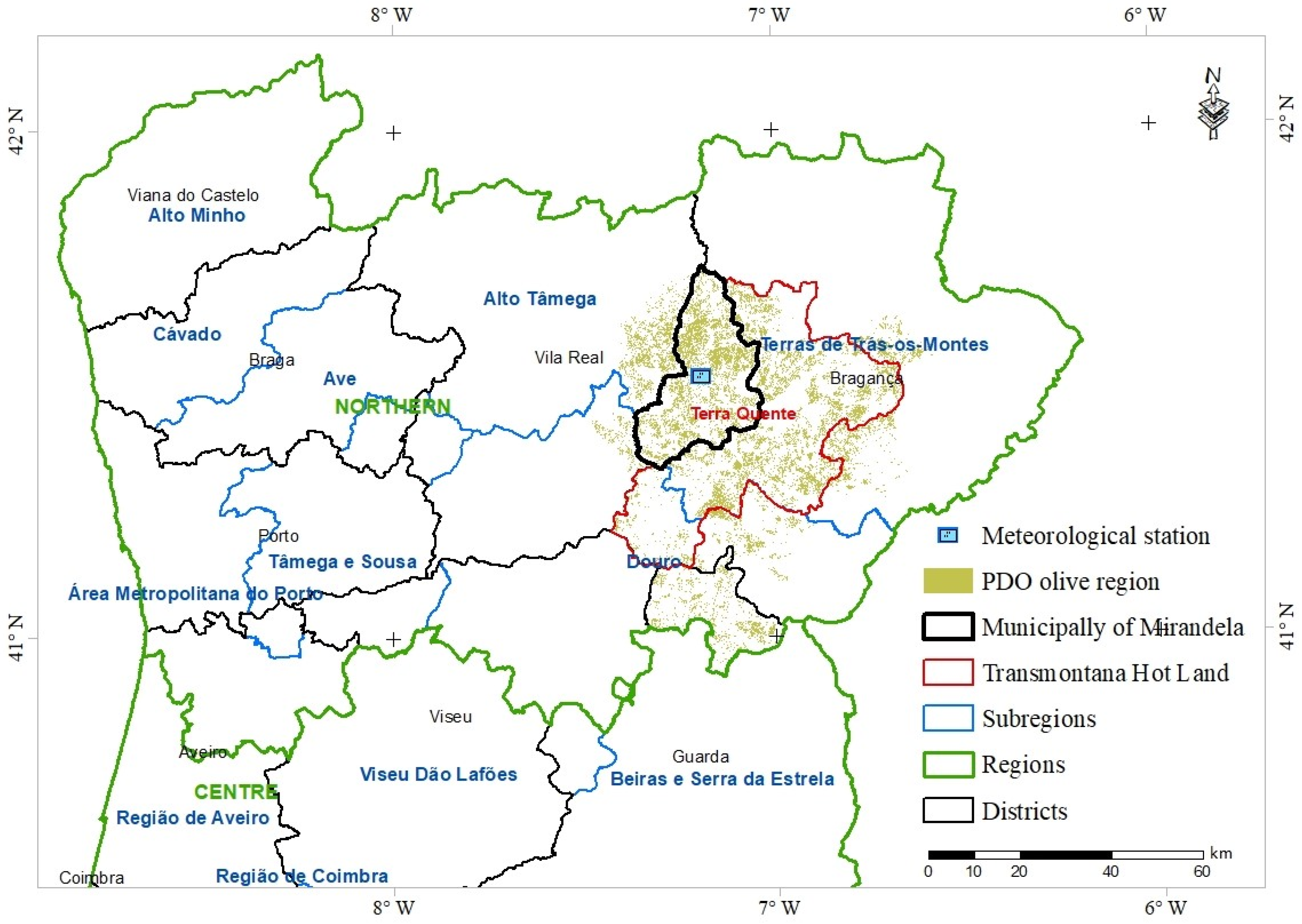
2.1. Study Area
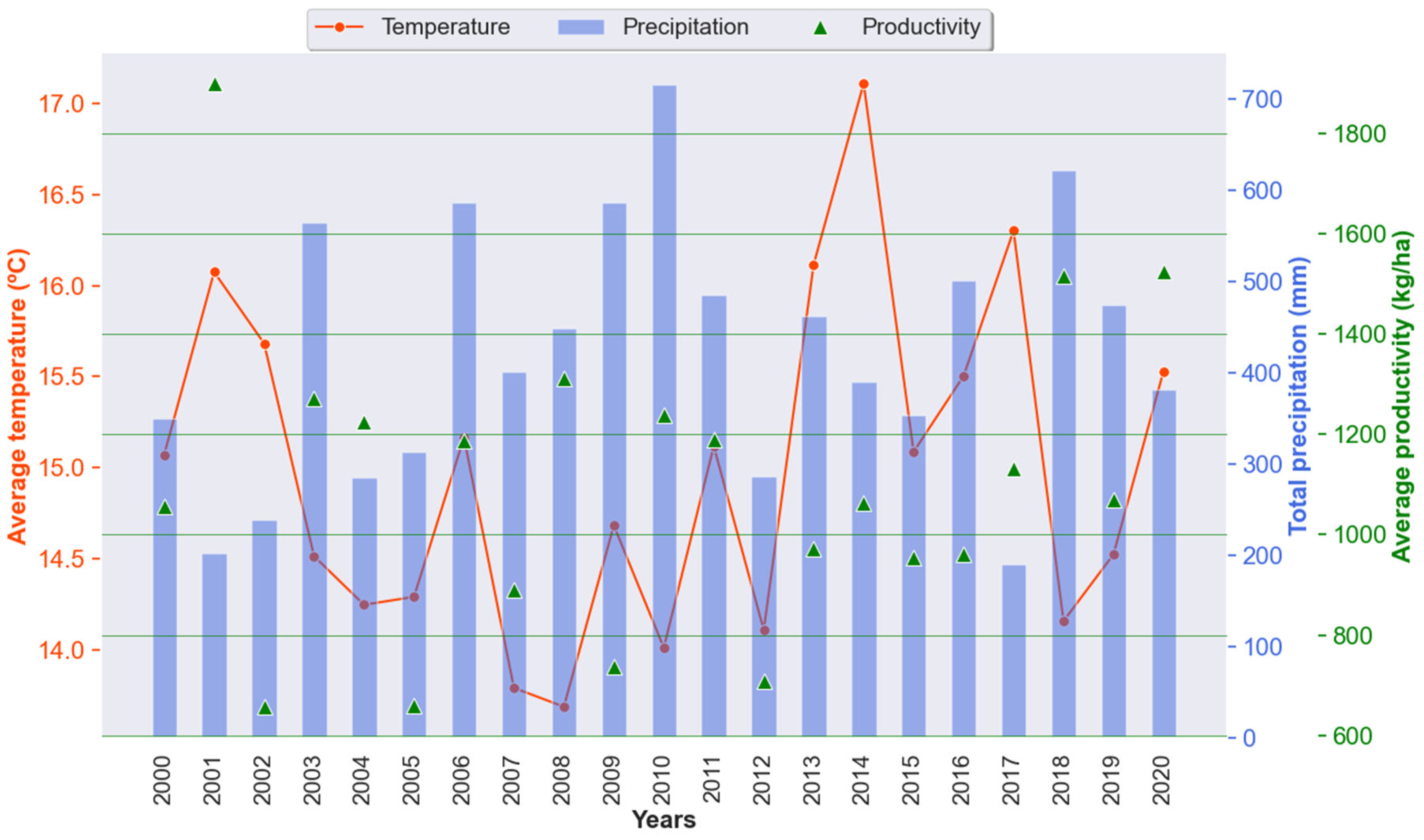
2.2. Climate and Olive Productivity Data
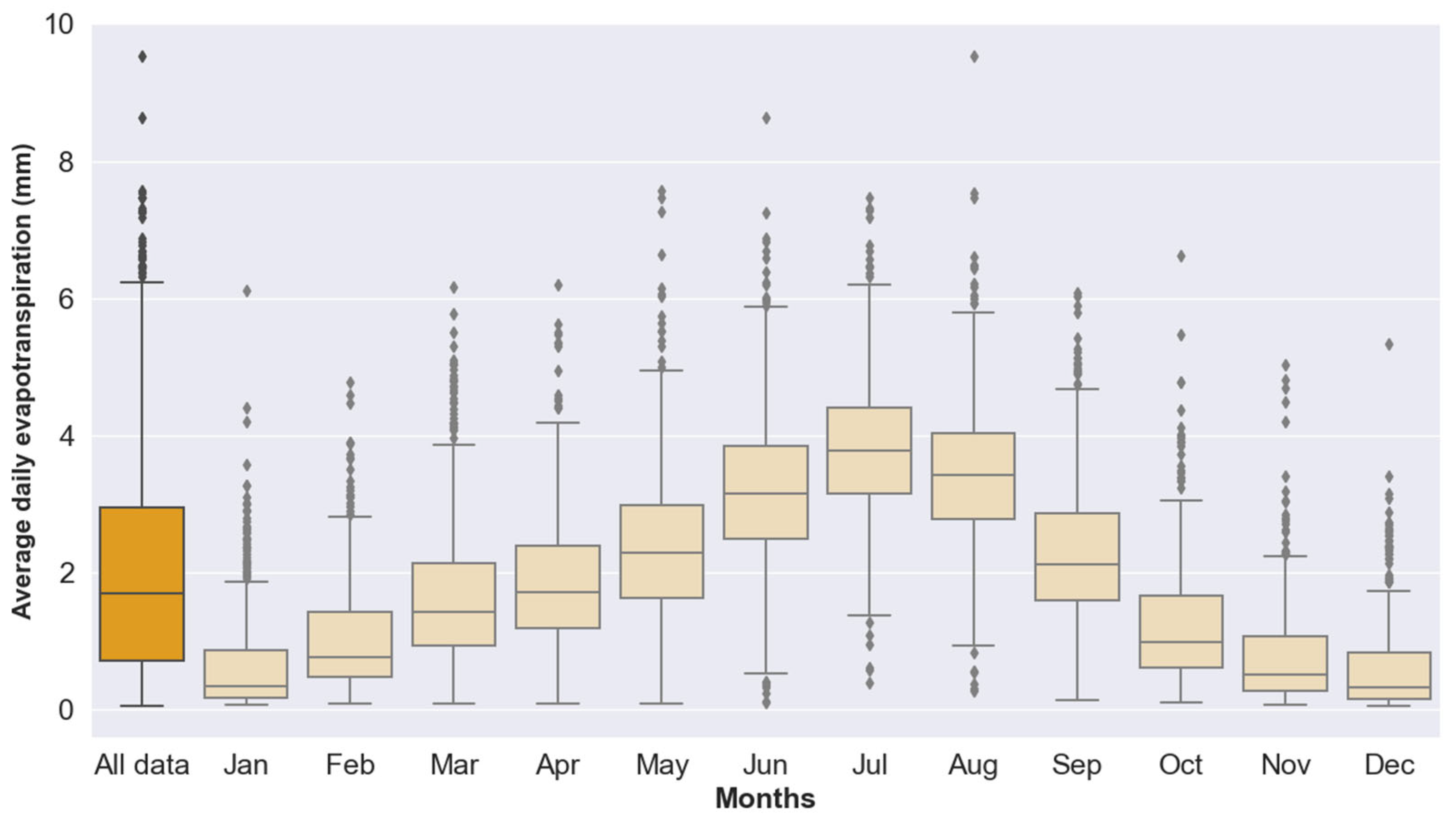
- The combined effect of all variables determines the crop evapotranspiration (ET) rate and consequent changes in its phenology and final yield;
- In Mediterranean climates, olive production greatly depends on the efficient use of winter and spring rainfall [3];
- Olive growing areas with well-illuminated canopies (i.e., that receive high radiation) tend to produce a greater quantity and quality of olive oil [5];
- Extreme-temperature anomalies, such as heat and cold spells, may have severe impacts on olive yields, occasionally leading to the death of olive trees.
2.3. Agro-Bioclimatic Indicators
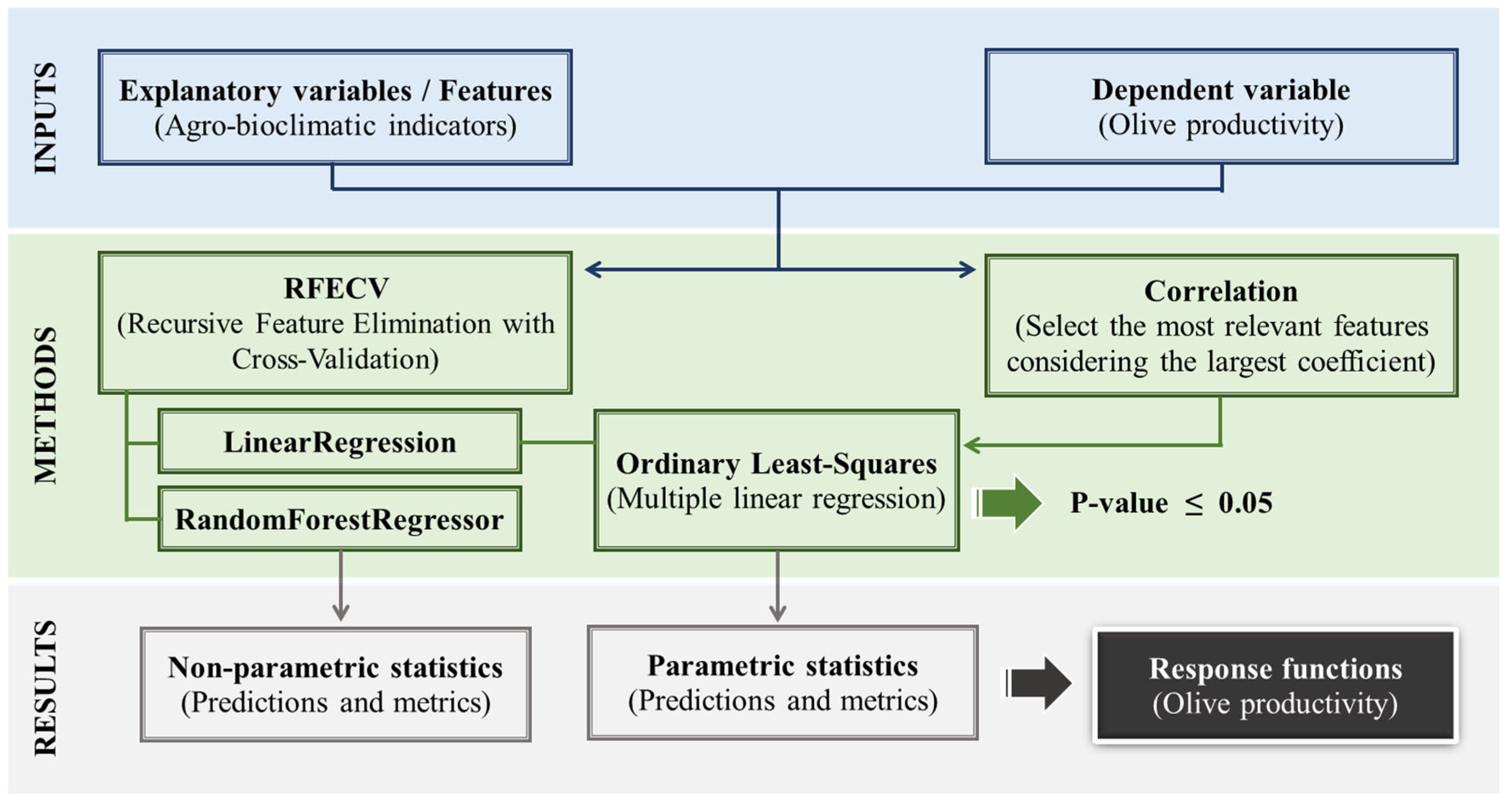
2.4. Regression Modeling
3. Results and Discussion
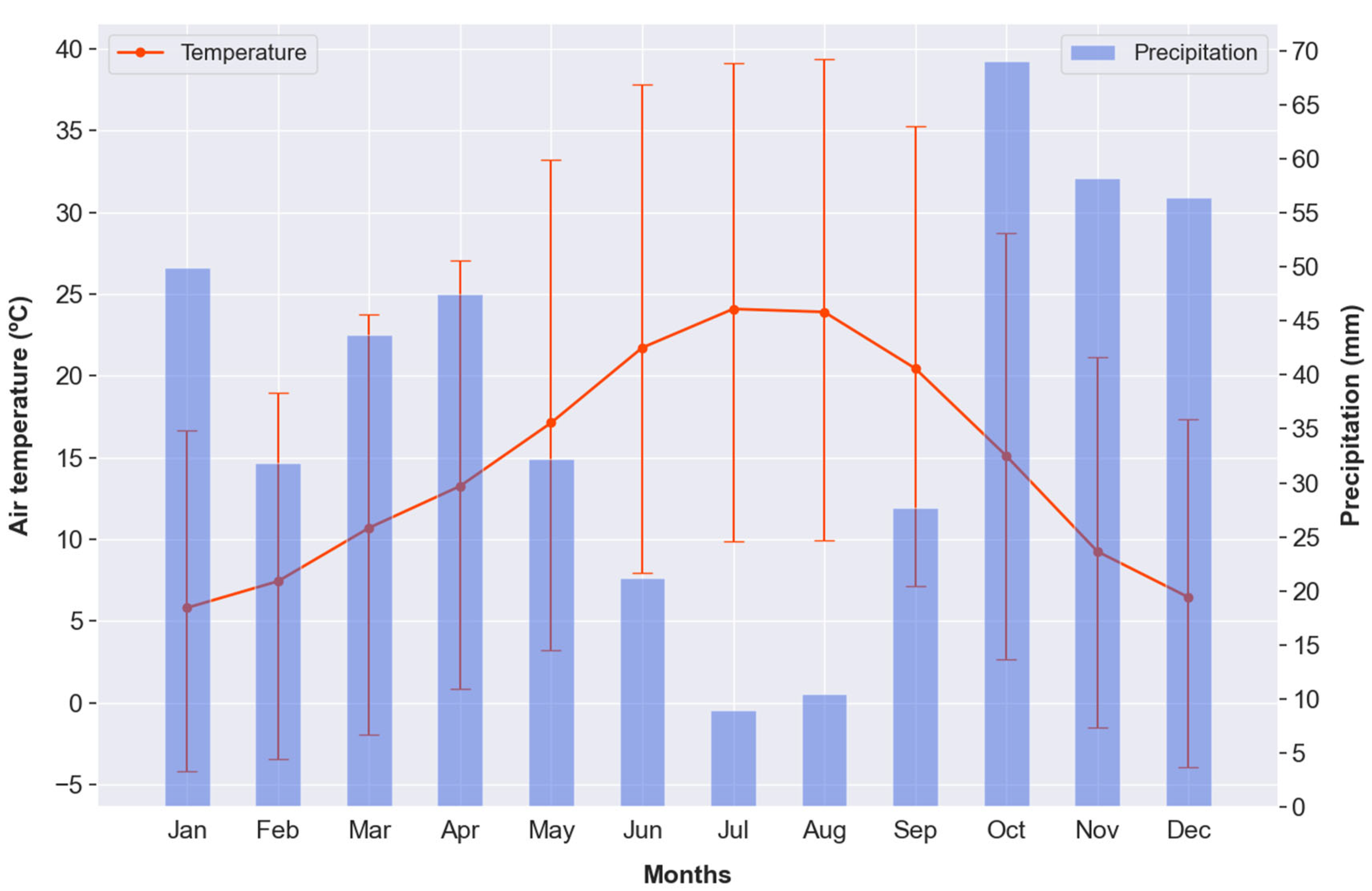
3.1. Agro-Bioclimatic Analysis
3.2. Crop Yield Response to Bioclimatic Variability
- OLS-LR (six features)—Ios2, Ios3, Ios4, Ia, SU40, and HW;
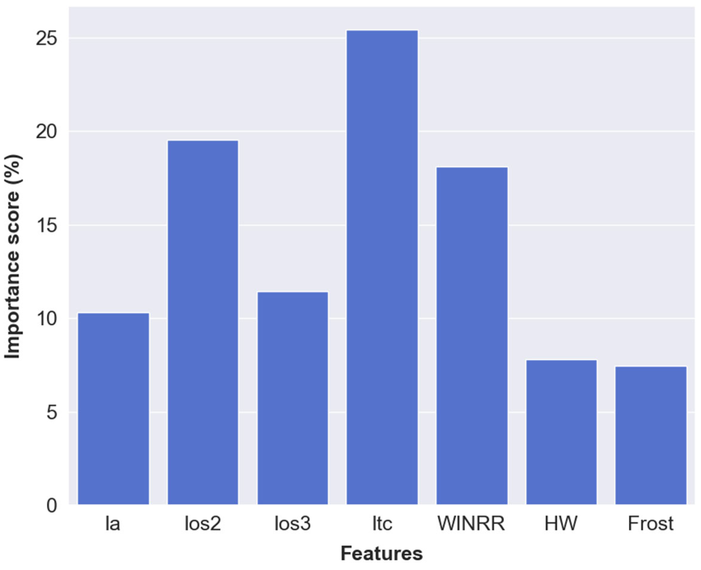
- RF (seven features)—Ia, Ios2, Ios3, Itc, WINRR, HW, and Frost.
4. Conclusions
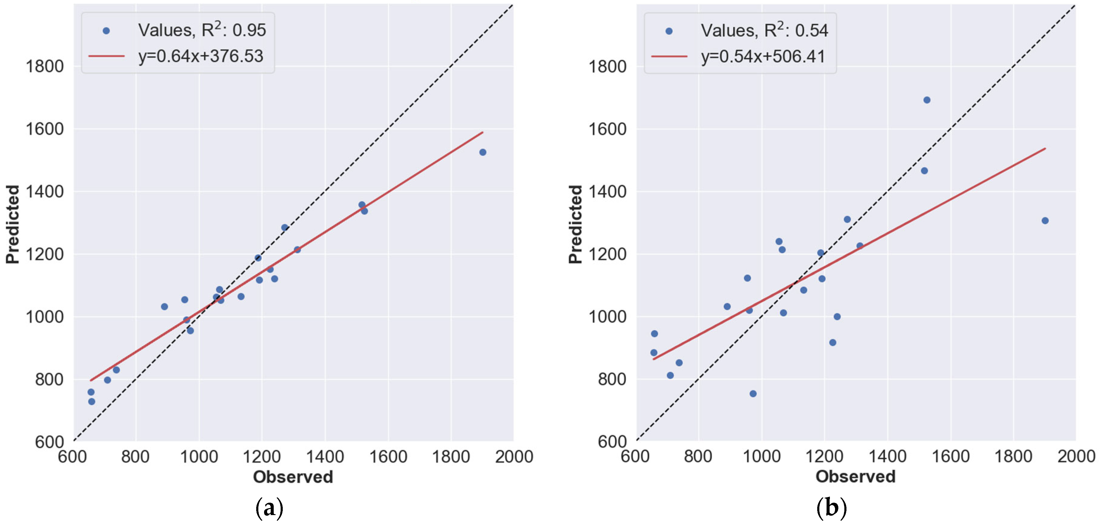
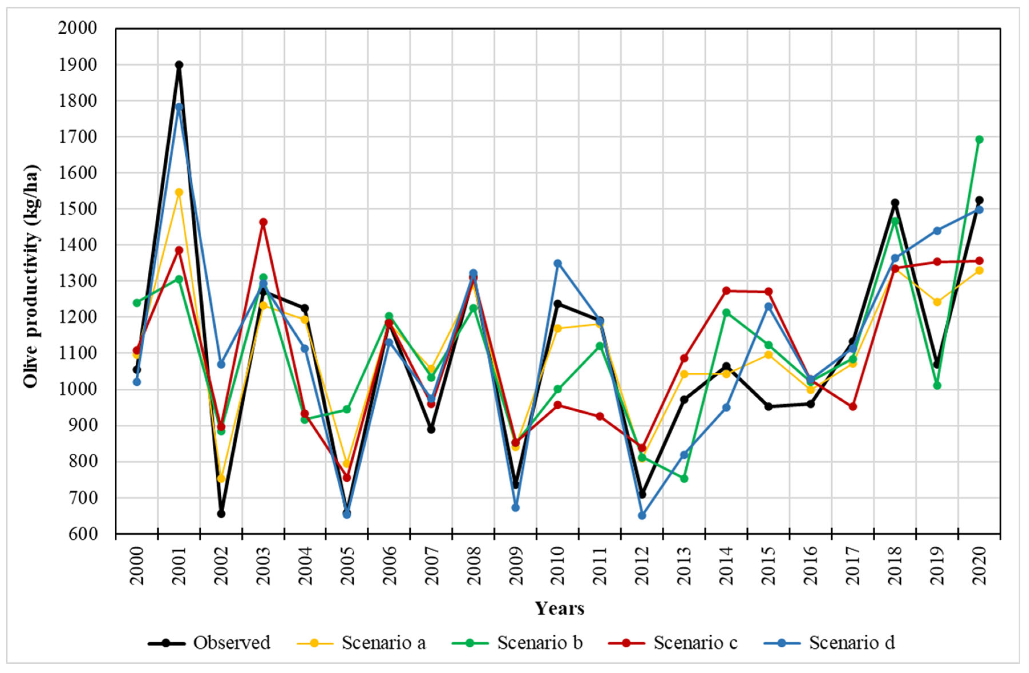
- The best statistical performance was achieved using the RF nonlinear approach with the most relevant features selected from the RFECV technique. However, given the underlying methodology, it was not possible to derive a regression model (a scenario);
- In OLS linear regression applications, the best agreement between the observed and predicted values was found when all analyzed features were added to the model run (d scenario);
- When using only the features selected through the RFECV and correlation techniques, the OLS model performance was substantially lower (b and c scenarios).
Author Contributions
Funding
Acknowledgments
Conflicts of Interest
References
- Rodrigo-Comino, J.; Salvia, R.; Quaranta, G.; Cudlín, P.; Salvati, L.; Gimenez-Morera, A. Climate Aridity and the Geographical Shift of Olive Trees in a Mediterranean Northern Region. Climate 2021, 9, 64. [Google Scholar] [CrossRef]
- Brito, C.; Dinis, L.T.; Moutinho-Pereira, J.; Correia, C.M. Drought Stress Effects and Olive Tree Acclimation under a Changing Climate. Plants 2019, 8, 232. [Google Scholar] [CrossRef]
- Fraga, H.; Moriondo, M.; Leolini, L.; Santos, J.A. Mediterranean Olive Orchards under Climate Change: A Review of Future Impacts and Adaptation Strategies. Agronomy 2020, 11, 56. [Google Scholar] [CrossRef]
- Tanasijevic, L.; Todorovic, M.; Pereira, L.S.; Pizzigalli, C.; Lionello, P. Impacts of climate change on olive crop evapotranspiration and irrigation requirements in the Mediterranean region. Agric. Water Manag. 2014, 144, 54–68. [Google Scholar] [CrossRef]
- Fernández, J.E. Understanding olive adaptation to abiotic stresses as a tool to increase crop performance. Environ. Exp. Bot. 2014, 103, 158–179. [Google Scholar] [CrossRef]
- Ponti, L.; Gutierrez, A.P.; Ruti, P.M.; Dell’Aquila, A. Fine-scale ecological and economic assessment of climate change on olive in the Mediterranean Basin reveals winners and losers. Proc. Natl. Acad. Sci. USA 2014, 111, 5598–5603. [Google Scholar] [CrossRef] [PubMed]
- De Luca, A.I.; Falcone, G.; Stillitano, T.; Iofrida, N.; Strano, A.; Gulisano, G. Evaluation of sustainable innovations in olive growing systems: A Life Cycle Sustainability Assessment case study in southern Italy. J. Clean. Prod. 2018, 171, 1187–1202. [Google Scholar] [CrossRef]
- Ben Abdallah, S.; Parra-López, C.; Elfkih, S.; Suárez-Rey, E.M.; Romero-Gámez, M. Sustainability assessment of traditional, intensive and highly-intensive olive growing systems in Tunisia by integrating Life Cycle and Multicriteria Decision analyses. Sustain. Prod. Consum. 2022, 33, 73–87. [Google Scholar] [CrossRef]
- Mairech, H.; López-Bernal, Á.; Moriondo, M.; Dibari, C.; Regni, L.; Proietti, P.; Villalobos, F.J.; Testi, L. Is new olive farming sustainable? A spatial comparison of productive and environmental performances between traditional and new olive orchards with the model OliveCan. Agric. Syst. 2020, 181, 102816. [Google Scholar] [CrossRef]
- Duarte, F.; Jones, N.; Fleskens, L. Traditional olive orchards on sloping land: Sustainability or abandonment? J. Environ. Manag. 2008, 89, 86–98. [Google Scholar] [CrossRef]
- Romero-Gámez, M.; Castro-Rodríguez, J.; Suárez-Rey, E.M. Optimization of olive growing practices in Spain from a life cycle assessment perspective. J. Clean. Prod. 2017, 149, 25–37. [Google Scholar] [CrossRef]
- Stroosnijder, L.; Mansinho, M.I.; Palese, A.M. OLIVERO: The project analysing the future of olive production systems on sloping land in the Mediterranean basin. J. Environ. Manag. 2008, 89, 75–85. [Google Scholar] [CrossRef] [PubMed]
- Silveira, C.; Almeida, A.; Ribeiro, A.C. Technological Innovation in the Traditional Olive Orchard Management: Advances and Opportunities to the Northeastern Region of Portugal. Water 2022, 14, 4081. [Google Scholar] [CrossRef]
- Morales, A.; Leffelaar, P.A.; Testi, L.; Orgaz, F.; Villalobos, F.J. A dynamic model of potential growth of olive (Olea europaea L.) orchards. Eur. J. Agron. 2016, 74, 93–102. [Google Scholar] [CrossRef]
- López-Bernal, Á.; Morales, A.; García-Tejera, O.; Testi, L.; Orgaz, F.; De Melo-Abreu, J.P.; Villalobos, F.J. OliveCan: A process-based model of development, growth and yield of olive orchards. Front. Plant Sci. 2018, 9, 632. [Google Scholar] [CrossRef]
- Sousa, A.A.R.; Barandica, J.M.; Aguilera, P.A.; Rescia, A.J. Examining Potential Environmental Consequences of Climate Change and Other Driving Forces on the Sustainability of Spanish Olive Groves under a Socio-Ecological Approach. Agriculture 2020, 10, 509. [Google Scholar] [CrossRef]
- Orlandi, F.; Garcia-Mozo, H.; Dhiab, A.B.; Galán, C.; Msallem, M.; Romano, B.; Abichou, M.; Dominguez-Vilches, E.; Fornaciari, M. Climatic indices in the interpretation of the phenological phases of the olive in mediterranean areas during its biological cycle. Clim. Chang. 2013, 116, 263–284. [Google Scholar] [CrossRef]
- Lorite, I.J.; Gabaldón-Leal, C.; Ruiz-Ramos, M.; Belaj, A.; de la Rosa, R.; León, L.; Santos, C. Evaluation of olive response and adaptation strategies to climate change under semi-arid conditions. Agric. Water Manag. 2018, 204, 247–261. [Google Scholar] [CrossRef]
- Osborne, C.P.; Chuine, I.; Viner, D.; Woodward, F.I. Olive phenology as a sensitive indicator of future climatic warming in the Mediterranean. Plant. Cell Environ. 2000, 23, 701–710. [Google Scholar] [CrossRef]
- Oteros, J.; García-Mozo, H.; Vázquez, L.; Mestre, A.; Domínguez-Vilches, E.; Galán, C. Modelling olive phenological response to weather and topography. Agric. Ecosyst. Environ. 2013, 179, 62–68. [Google Scholar] [CrossRef]
- Arenas-Castro, S.; Gonçalves, J.F.; Moreno, M.; Villar, R. Projected climate changes are expected to decrease the suitability and production of olive varieties in southern Spain. Sci. Total Environ. 2020, 709, 136161. [Google Scholar] [CrossRef]
- Orlandi, F.; Rojo, J.; Picornell, A.; Oteros, J.; Pérez-Badia, R.; Fornaciari, M. Impact of Climate Change on Olive Crop Production in Italy. Atmosphere 2020, 11, 595. [Google Scholar] [CrossRef]
- Bussotti, F.; Ferrini, F.; Pollastrini, M.; Fini, A. The challenge of Mediterranean sclerophyllous vegetation under climate change: From acclimation to adaptation. Environ. Exp. Bot. 2014, 103, 80–98. [Google Scholar] [CrossRef]
- Fraga, H.; Pinto, J.G.; Santos, J.A. Climate change projections for chilling and heat forcing conditions in European vineyards and olive orchards: A multi-model assessment. Clim. Chang. 2018, 152, 179–193. [Google Scholar] [CrossRef]
- García-Inza, G.P.; Castro, D.N.; Hall, A.J.; Rousseaux, M.C. Responses to temperature of fruit dry weight, oil concentration, and oil fatty acid composition in olive (Olea europaea L. var. ‘Arauco’). Eur. J. Agron. 2014, 54, 107–115. [Google Scholar] [CrossRef]
- López-Bernal, Á.; Fernandes-Silva, A.A.; Vega, V.A.; Hidalgo, J.C.; León, L.; Testi, L.; Villalobos, F.J. A fruit growth approach to estimate oil content in olives. Eur. J. Agron. 2021, 123, 126206. [Google Scholar] [CrossRef]
- Viola, F.; Valerio Noto, L.; Cannarozzo, M.; La Loggia, G.; Porporato, A. Olive yield as a function of soil moisture dynamics. Ecohydrology 2012, 5, 99–107. [Google Scholar] [CrossRef]
- Cabezas, J.M.; Ruiz-Ramos, M.; Soriano, M.A.; Gabaldón-Leal, C.; Santos, C.; Lorite, I.J. Identifying adaptation strategies to climate change for Mediterranean olive orchards using impact response surfaces. Agric. Syst. 2020, 185, 102937. [Google Scholar] [CrossRef]
- Mairech, H.; López-Bernal, Á.; Moriondo, M.; Dibari, C.; Regni, L.; Proietti, P.; Villalobos, F.J.; Testi, L. Sustainability of olive growing in the Mediterranean area under future climate scenarios: Exploring the effects of intensification and deficit irrigation. Eur. J. Agron. 2021, 129, 126319. [Google Scholar] [CrossRef]
- Caselli, A.; Petacchi, R. Climate Change and Major Pests of Mediterranean Olive Orchards: Are We Ready to Face the Global Heating? Insects 2021, 12, 802. [Google Scholar] [CrossRef] [PubMed]
- Moriondo, M.; Trombi, G.; Ferrise, R.; Brandani, G.; Dibari, C.; Ammann, C.M.; Lippi, M.M.; Bindi, M. Olive trees as bio-indicators of climate evolution in the Mediterranean Basin. Glob. Ecol. Biogeogr. 2013, 22, 818–833. [Google Scholar] [CrossRef]
- Zagaria, C.; Schulp, C.J.E.; Malek, Ž.; Verburg, P.H. Potential for land and water management adaptations in Mediterranean croplands under climate change. Agric. Syst. 2023, 205, 103586. [Google Scholar] [CrossRef]
- Cano-Ortiz, A.; Carlos, J.; Fuentes, P.; Leiva Gea, F.; Mahmoud, J.; Ighbareyeh, H.; Jorje, R.; Canas, Q.; Isabel, C.; Meireles, R.; et al. Climatology, Bioclimatology and Vegetation Cover: Tools to Mitigate Climate Change in Olive Groves. Agronomy 2022, 12, 2707. [Google Scholar] [CrossRef]
- INE Statistics Portugal. Available online: https://www.ine.pt (accessed on 4 February 2023).
- Andrade, C.; Fonseca, A.; Santos, J.A. Are land use options in viticulture and oliviculture in agreement with bioclimatic shifts in portugal? Land 2021, 10, 869. [Google Scholar] [CrossRef]
- DGT. A Land Cover/Use Map of Mainland Portugal for 2018; Directorate-General for the Territorial Development: Lisbon, Portugal, 2019. [Google Scholar]
- IPMA. Weather Stations Network. Available online: https://www.ipma.pt/en/otempo/obs.superficie/#Mirandela (accessed on 20 January 2023).
- Bonofiglio, T.; Orlandi, F.; Ruga, L.; Romano, B.; Fornaciari, M. Climate change impact on the olive pollen season in Mediterranean areas of Italy: Air quality in late spring from an allergenic point of view. Environ. Monit. Assess. 2013, 185, 877–890. [Google Scholar] [CrossRef] [PubMed]
- Bonofiglio, T.; Orlandi, F.; Sgromo, C.; Romano, B.; Fornaciari, M. Influence of temperature and rainfall on timing of olive (Olea europaea) flowering in southern Italy. N. Z. J. Crop Hortic. Sci. 2008, 36, 59–69. [Google Scholar] [CrossRef]
- Rivas-Martínez, S.; Sáenz, S.R.; Penas, A. Worldwide Bioclimatic Classification System. Glob. Geobot. 2011, 1, 1–634. [Google Scholar] [CrossRef]
- Gratsea, M.; Varotsos, K.V.; López-Nevado, J.; López-Feria, S.; Giannakopoulos, C. Assessing the long-term impact of climate change on olive crops and olive fly in Andalusia, Spain, through climate indices and return period analysis. Clim. Serv. 2022, 28, 100325. [Google Scholar] [CrossRef]
- Allen, R.G.; Pereira, L.S.; Raes, D.; Smith, M. Crop Evapotranspiration-Guidelines for Computing Crop Water Requirements-FAO Irrigation and Drainage Paper 56; FAO: Rome, Italy, 1998. [Google Scholar]
- Russo, S.; Dosio, A.; Graversen, R.G.; Sillmann, J.; Carrao, H.; Dunbar, M.B.; Singleton, A.; Montagna, P.; Barbola, P.; Vogt, J.V.; et al. Magnitude of extreme heat waves in present climate and their projection in a warming world. J. Geophys. Res. Atmos. 2014, 119, 12500–12512. [Google Scholar] [CrossRef]
- Pereira, S.C.; Marta-Almeida, M.; Carvalho, A.C.; Rocha, A. Heat wave and cold spell changes in Iberia for a future climate scenario. Int. J. Climatol. 2017, 37, 5192–5205. [Google Scholar] [CrossRef]
- Awada, H.; Di Prima, S.; Sirca, C.; Giadrossich, F.; Marras, S.; Spano, D.; Pirastru, M. Daily Actual Evapotranspiration Estimation in a Mediterranean Ecosystem from Landsat Observations Using SEBAL Approach. Forests 2021, 12, 189. [Google Scholar] [CrossRef]
- Pereira, L.S.; Paredes, P.; López-Urrea, R.; Hunsaker, D.J.; Mota, M.; Mohammadi Shad, Z. Standard single and basal crop coefficients for vegetable crops, an update of FAO56 crop water requirements approach. Agric. Water Manag. 2021, 243, 106196. [Google Scholar] [CrossRef]
- Salgado, R.; Mateos, L. Evaluation of different methods of estimating ET for the performance assessment of irrigation schemes. Agric. Water Manag. 2021, 243, 106450. [Google Scholar] [CrossRef]
- Paulo, A.A.; Rosa, R.D.; Pereira, L.S. Climate trends and behaviour of drought indices based on precipitation and evapotranspiration in Portugal. Nat. Hazards Earth Syst. Sci. 2012, 12, 1481–1491. [Google Scholar] [CrossRef]
- Zomer, R.J.; Xu, J.; Trabucco, A. Version 3 of the Global Aridity Index and Potential Evapotranspiration Database. Sci. Data 2022, 9, 409. [Google Scholar] [CrossRef]
- Porter, J.R.; Semenov, M.A. Crop responses to climatic variation. Philos. Trans. R. Soc. B Biol. Sci. 2005, 360, 2021–2035. [Google Scholar] [CrossRef] [PubMed]
- Scikit-learn, D. Recursive Feature Elimination with Cross-Validation to Select Features. Available online: https://scikit-learn.org/stable/modules/generated/sklearn.feature_selection.RFECV.html (accessed on 10 March 2023).
- Scikit-learn, D. Ordinary Least Squares Linear Regression. Available online: https://scikit-learn.org/stable/modules/generated/sklearn.linear_model.LinearRegression.html (accessed on 8 May 2023).
- Scikit-learn, D. A Random Forest Regressor. Available online: https://scikit-learn.org/stable/modules/generated/sklearn.ensemble.RandomForestRegressor.html (accessed on 12 March 2023).
- Rencher, A.C.; Schaalje, G.B. Linear Models in Statistics; John Wiley and Sons: Hoboken, NJ, USA, 2007; ISBN 9780471754985. [Google Scholar]
- Cutler, A.; Cutler, D.R.; Stevens, J.R. Random forests. In Ensemble Machine Learning, 2nd ed.; Zhang, C., Ma, Y.Q., Eds.; Springer: New York, NY, USA, 2012; pp. 157–175. [Google Scholar] [CrossRef]
- Cherlet, M.; Hutchinson, C.; Reynolds, J.; Hill, J.; Sommer, S.; von Maltitz, G. World Atlas of Desertification; Publication Office of the European Union: Luxembourg, 2018; ISBN 978-92-79-75350-3. [Google Scholar]
- Andrade, C.; Contente, J. Climate change projections for the Worldwide Bioclimatic Classification System in the Iberian Peninsula until 2070. Int. J. Climatol. 2020, 40, 5863–5886. [Google Scholar] [CrossRef]
- Di Paola, A.; Di Giuseppe, E.; Gutierrez, A.P.; Ponti, L.; Pasqui, M. Climate stressors modulate interannual olive yield at province level in Italy: A composite index approach to support crop management. J. Agron. Crop Sci. 2023, 1–14. [Google Scholar] [CrossRef]
- Fraga, H.; Molitor, D.; Leolini, L.; Santos, J.A. What Is the Impact of Heatwaves on European Viticulture? A Modelling Assessment. Appl. Sci. 2020, 10, 3030. [Google Scholar] [CrossRef]
- Ascenso, A.; Gama, C.; Blanco-Ward, D.; Monteiro, A.; Silveira, C.; Viceto, C.; Rodrigues, V.; Rocha, A.; Borrego, C.; Lopes, M.; et al. Assessing Douro Vineyards Exposure to Tropospheric Ozone. Atmosphere 2021, 12, 200. [Google Scholar] [CrossRef]


| Indicators | Description and Units |
|---|---|
| Climatic parameters | |
| T | Average annual temperature [°C] |
| Ti | Average monthly temperature [°C], where i is the month of the year |
| Tmax | Average temperature of the hottest month [°C] |
| Tmin | Average temperature of the coldest month [°C] |
| M | Average temperature of the daily maximums of the coldest month [°C] |
| m | Average temperature of the daily minimums of the coldest month [°C] |
| Tp | Positive annual temperature: total in tenths of °C when Ti is higher than 0 °C, ∑Ti > 0°C |
| P | Annual precipitation [mm] |
| Pi | Monthly precipitation [mm], where i is the month of the year |
| Pp | Positive annual precipitation of the months with a Ti higher than 0 °C, ∑Pi when Ti > 0°C |
| Bioclimatic indices | |
| ETo | Average annual reference evapotranspiration [mm]: calculated using the FAO56 Penman–Monteith method [42] |
| Ia | Annual aridity index, Ia = P/ETo |
| Ios1 | Ombrothermic index of the hottest summer month, Ios1 = (Pi/Ti) × 10 |
| Ios2 | Ombrothermic index of the hottest summer bimester |
| Ios3 | Ombrothermic index of the summer trimester (Jun–Aug) |
| Ios4 | Compensated summer ombrothermic index: by adding the month immediately preceding to the summer trimester |
| Ic | Simple continentality index [°C]: Annual thermal amplitude, Ic = Tmax − Tmin |
| Itc | Compensated thermicity index [°C], Itc = (T + m + M) × 10 ± f(Ic) |
| WINRR | Total precipitation from October to May [mm]: water deficit during this period may strongly reduce the olive yield |
| SPRTX | Average temperature of the daily maximums during the springtime (Apr–May) [°C]: considered the best indicator of flowering date in olive trees |
| Extreme weather events | |
| SPR32 | Number of spring days with maximum temperature higher than 32 °C: connected to early flowering of the olive tree |
| SU36 | Number of summer days with maximum temperature higher than 36 °C: related to early olive ripening |
| SU40 | Number of summer days with maximum temperature higher than 40 °C: limits the photosynthetic rate of the olive tree |
| HW | Heat wave magnitude index: annual count of days with at least 3 consecutive hot days of maximum temperature above the 90th percentile of daily maxima in a 31-day moving window (15 days on either side) [43,44] |
| Frost | Number of frost days: annual count of days with minimum temperature less than 0 °C |
| Icing | Number of icing days: annual count of days with maximum temperature less than 0 °C |
| Year | ETo | Ia | Ios1 | Ios2 | Ios3 | Ios4 | Ios3/Ios2 | Ic | Itc | WINRR | SPRTX | SPR32 | SU36 | SU40 | HW | Frost | Icing |
|---|---|---|---|---|---|---|---|---|---|---|---|---|---|---|---|---|---|
| 2000 | 1159.6 | 0.3 | 0.9 | 0.5 | 0.4 | 1.2 | 0.9 | 19.2 | 244.0 | 374.6 | 19.2 | 7 | 12 | 0 | 0 | 27 | 0 |
| 2001 | 1213.8 | 0.2 | 0.5 | 0.8 | 0.5 | 1.0 | 0.7 | 20.5 | 232.2 | 204.3 | 21.8 | 13 | 11 | 0 | 3 | 29 | 2 |
| 2002 | 1000.8 | 0.2 | 0.0 | 0.0 | 0.2 | 0.4 | 0.0 | 16.4 | 291.1 | 137.1 | 21.2 | 11 | 8 | 0 | 0 | 18 | 0 |
| 2003 | 883.7 | 0.6 | 0.7 | 1.2 | 0.9 | 0.8 | 0.8 | 20.8 | 273.0 | 317.0 | 18.4 | 9 | 15 | 6 | 12 | 24 | 1 |
| 2004 | 1194.0 | 0.2 | 0.4 | 0.3 | 0.6 | 0.8 | 2.1 | 19.3 | 269.7 | 362.2 | 21.4 | 15 | 9 | 0 | 0 | 42 | 0 |
| 2005 | 1319.5 | 0.2 | 0.0 | 0.1 | 0.1 | 0.3 | 1.5 | 21.0 | 253.2 | 279.4 | 22.1 | 16 | 22 | 1 | 3 | 72 | 0 |
| 2006 | 1156.2 | 0.5 | 0.8 | 0.7 | 1.1 | 1.0 | 1.6 | 21.6 | 276.2 | 333.2 | 23.6 | 11 | 18 | 0 | 4 | 48 | 1 |
| 2007 | 1075.2 | 0.4 | 1.5 | 1.0 | 1.5 | 1.9 | 1.5 | 18.1 | 245.8 | 501.9 | 22.1 | 2 | 7 | 1 | 0 | 48 | 0 |
| 2008 | 1051.1 | 0.4 | 1.3 | 0.7 | 0.9 | 1.4 | 1.2 | 17.9 | 248.7 | 332.1 | 19.5 | 2 | 7 | 0 | 0 | 38 | 4 |
| 2009 | 1270.6 | 0.5 | 0.1 | 0.1 | 0.8 | 0.9 | 13.1 | 18.4 | 287.7 | 256.5 | 22.5 | 12 | 13 | 0 | 0 | 39 | 0 |
| 2010 | 1047.3 | 0.7 | 0.0 | 0.0 | 0.6 | 0.7 | 0.0 | 20.7 | 280.9 | 733.2 | 21.7 | 7 | 24 | 1 | 3 | 41 | 0 |
| 2011 | 1069.6 | 0.5 | 0.6 | 0.3 | 0.2 | 0.2 | 0.8 | 17.5 | 290.4 | 560.8 | 25.8 | 7 | 15 | 1 | 3 | 31 | 0 |
| 2012 | 1164.1 | 0.2 | 0.2 | 0.3 | 0.3 | 0.7 | 1.3 | 19.6 | 249.5 | 260.2 | 20.8 | 5 | 20 | 3 | 3 | 56 | 0 |
| 2013 | 1144.4 | 0.4 | 0.0 | 0.0 | 0.1 | 0.4 | 7.5 | 19.6 | 314.5 | 458.2 | 20.3 | 1 | 26 | 6 | 9 | 18 | 0 |
| 2014 | 869.1 | 0.4 | 1.8 | 0.9 | 0.9 | 0.9 | 1.0 | 18.4 | 297.3 | 135.8 | 24.6 | 6 | 8 | 0 | 0 | 11 | 0 |
| 2015 | 1213.0 | 0.3 | 0.6 | 0.7 | 0.5 | 0.7 | 0.7 | 22.3 | 282.2 | 300.6 | 24.3 | 16 | 23 | 4 | 9 | 34 | 0 |
| 2016 | 785.0 | 0.6 | 0.2 | 0.1 | 0.2 | 1.4 | 2.0 | 17.9 | 335.2 | 629.5 | 19.5 | 5 | 29 | 6 | 6 | 15 | 0 |
| 2017 | 1218.0 | 0.2 | 0.0 | 0.1 | 0.4 | 0.6 | 7.1 | 19.5 | 299.5 | 101.5 | 25.6 | 18 | 20 | 3 | 15 | 35 | 0 |
| 2018 | 940.7 | 0.7 | 0.1 | 1.8 | 1.4 | 1.5 | 0.8 | 19.1 | 286.1 | 419.3 | 22.0 | 5 | 15 | 4 | 5 | 34 | 0 |
| 2019 | 1281.8 | 0.4 | 0.3 | 0.9 | 0.9 | 0.7 | 1.0 | 21.1 | 253.6 | 295.0 | 22.5 | 6 | 15 | 1 | 0 | 50 | 3 |
| 2020 | 1213.3 | 0.3 | 0.5 | 0.9 | 0.7 | 0.8 | 0.7 | 21.0 | 308.3 | 468.0 | 23.5 | 9 | 31 | 0 | 12 | 19 | 0 |
| Average | 1108.1 | 0.4 | 0.5 | 0.5 | 0.6 | 0.9 | 2.2 | 19.5 | 277.1 | 355.3 | 22.0 | 9 | 17 | 2 | 4 | 35 | 1 |
| Scenarios | Regression Models | R2 | MAE (kg/ha) | RMSE (kg/ha) |
|---|---|---|---|---|
| (a) RF with fitted RFECV features | Not applicable | 0.95 | 88.49 | 120.50 |
| (b) OLS with fitted RFECV features | 741.29 + 517.15 Ios2 − 520.02 Ios3 + 230.31 Ios4 + 597.23 Ia − 101.94 SU40 + 39.13 HW | 0.54 | 158.91 | 203.58 |
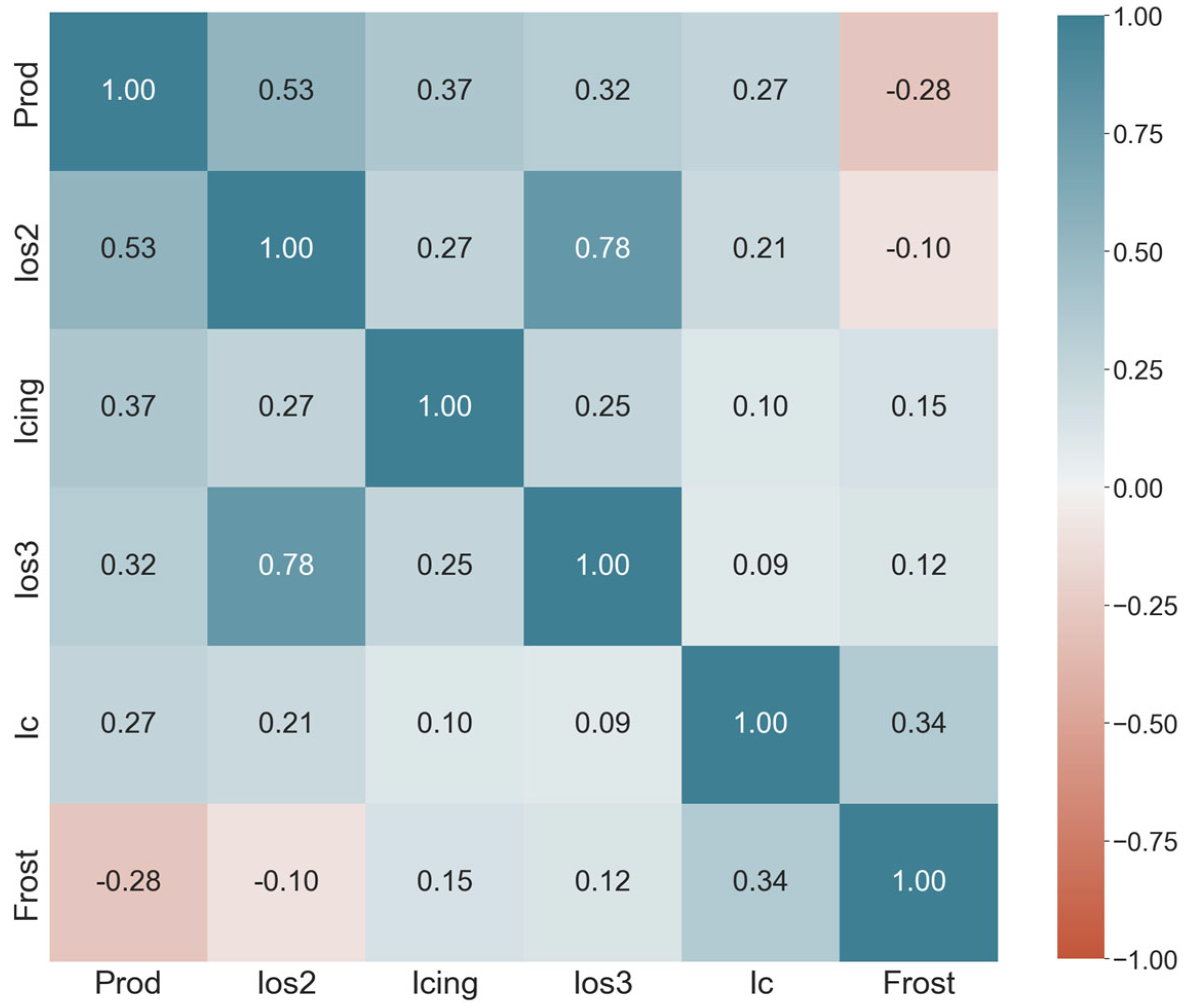
| (c) OLS with correlation features | 81.67 + 232.68 Ios2 + 82.81 Icing − 15.28 Ios3 − 7.92 Frost + 58.53 Ic | 0.49 | 179.88 | 215.66 |
| (d) OLS with all features | −4283.73 − 0.64 ETo + 330.01 Ia − 460.36 Ios1 + 389.87 Ios2 − 1150.86 Ios3 + 666.38 Ios4 + 249.21 Ic + 4.48 Itc + 0.82 WINRR + 56.93 SPRTX − 41.72 SPR32 − 73.39 SU36 − 144.60 SU40 + 76.49 HW − 0.35 Frost + 51.86 Icing | 0.85 | 86.23 | 115.75 |
Disclaimer/Publisher’s Note: The statements, opinions and data contained in all publications are solely those of the individual author(s) and contributor(s) and not of MDPI and/or the editor(s). MDPI and/or the editor(s) disclaim responsibility for any injury to people or property resulting from any ideas, methods, instructions or products referred to in the content. |
© 2023 by the authors. Licensee MDPI, Basel, Switzerland. This article is an open access article distributed under the terms and conditions of the Creative Commons Attribution (CC BY) license (https://creativecommons.org/licenses/by/4.0/).
Share and Cite
Silveira, C.; Almeida, A.; Ribeiro, A.C. How Can a Changing Climate Influence the Productivity of Traditional Olive Orchards? Regression Analysis Applied to a Local Case Study in Portugal. Climate 2023, 11, 123. https://doi.org/10.3390/cli11060123
Silveira C, Almeida A, Ribeiro AC. How Can a Changing Climate Influence the Productivity of Traditional Olive Orchards? Regression Analysis Applied to a Local Case Study in Portugal. Climate. 2023; 11(6):123. https://doi.org/10.3390/cli11060123
Chicago/Turabian StyleSilveira, Carlos, Arlindo Almeida, and António C. Ribeiro. 2023. "How Can a Changing Climate Influence the Productivity of Traditional Olive Orchards? Regression Analysis Applied to a Local Case Study in Portugal" Climate 11, no. 6: 123. https://doi.org/10.3390/cli11060123