

Identifying and Attributing Regime Shifts in Australian Fire Climates

Institute of Sustainable Industries and Liveable Cities, Victoria University Melbourne, Footscray, VIC 3011, Australia
*
Author to whom correspondence should be addressed.
Climate 2023, 11(6), 121; https://doi.org/10.3390/cli11060121
Submission received: 3 May 2023
/
Revised: 19 May 2023
/
Accepted: 22 May 2023
/
Published: 28 May 2023
(This article belongs to the Special Issue Recent Climate Change Impacts in Australia)
Abstract
:This paper introduces and analyzes fire climate regimes, steady-state conditions that govern the behavior of fire weather. A simple model representing fire climate was constructed by regressing high-quality regional climate averages against the station-averaged annual Forest Fire Danger Index (FFDI) for Victoria, Australia. Four FFD indices for fire years 1957–2021 were produced for 10 regions. Regions with even coverage of station-averaged total annual FFDI (ΣFFDI) from 1971–2016 exceeded Nash–Sutcliffe efficiencies of 0.84, validating its widespread application. Data were analyzed for shifts in mean, revealing regime shifts that occurred between 1996 and 2003 in the southern states and 2012–2013 in Queensland. ΣFFDI shifted up by ~25% in SE Australia to 8% in the west; by approximately one-third in the SE to 7% in the west for days above high fire danger; by approximately half in the SE to 11% in the west for days above very high, with a greater increase in Tasmania; and by approximately three-quarters in the SE to 9% in the west for days above severe FFDI. Attribution of the causes identified regime shifts in the fire season maximum temperature and a 3 p.m. relative humidity, with changing drought factor and rainfall patterns shaping the results. The 1:10 fire season between Regimes 1 and 2 saw a three to seven times increase with an average of five. For the 1:20 fire season, there was an increase of 2 to 14 times with an average of 8. Similar timing between shifts in the Australian FFDI and the global fire season length suggests that these changes may be global in extent. A trend analysis will substantially underestimate these changes in risk.
1. Introduction
Over the past two decades, Australia has experienced wildfires of increased frequency and severity due to climate change [1,2]. The 2019–2020 fire season, the black summer, was the worst on record for area burned and property loss [1,2]. Two outstanding issues in understanding the current level of fire risk are: how much of that risk is due to human-induced climate change, and how much of an increase do we need to plan for?
Both aspects are difficult to quantify. Fire risk indices require high-quality input data that are often unavailable. Existing data are of limited quality, spatial coverage, and continuity. The risk of wildfire also depends on land surface and cover conditions, and in response to increasingly severe fire weather, is also highly nonlinear. Bradstock [3] described four fire switches that dial up fire risk: biomass production, biomass readiness to burn, fire weather, and ignition sources. Climate influences all of these, the third most directly. All four are needed for a comprehensive assessment of fire risk at a given location [3]. The typical fire risk at a place taking account of these characteristics make up the generally accepted definition of a fire regime [4].
This paper focuses on understanding and quantifying the external climatic conditions that contribute to regional fire climate, i.e., the climate entering a region before considering its land use and land cover, level of fuel, dryness, and topography. The incoming regional climate is conditioned by processes on the wider land and ocean surface that are largely independent of local conditions. This largely concerns temperature and moisture availability which make up the hydroclimate.
Our starting definition is that a fire climate (pyroclimate) is the incoming climate external to a region that affects the propensity for wildfire to occur. This does not include the likelihood of ignition, which requires another layer of information. The pyroclimate is situated towards the hot and dry end of the hydroclimate where there is sufficient rainfall to accumulate biomass as fuel and sufficient heat for its growth, but not at the very dry extreme which is too arid. The starting hypothesis is that the partitioning between latent and sensible heat used to estimate runoff, e.g., [5,6] can be applied to fire danger indices, allowing relatively simple relationships to be constructed from mean climatological data.
Climate is often defined as the average of weather [7,8,9], but is also, sometimes in the same publication, defined as the state of the climate system [9]. This distinguishes climate as index from climate as agent [10]. If it is the former, a fire climate will be the average of fire weather over a given period, but in the latter, climate will provide the boundary conditions for fire weather. We investigate this distinction by exploring regime-like behavior in fire climate.
We used McArthur’s Forest Fire Danger Index (FFDI) [11,12,13] as the basis for developing fire climate regimes using high-quality regional data (HQD) from the Australian Bureau of Meteorology (BoM). It is an index originally calculated on a scale of 100 based on the 1939 Black Friday fires [11,12], but has since exceeded 100, with that level being categorized as catastrophic [14]. The four measures produced were the annual sum of the FFDI (ΣFFDI) and days above high (Days Hi+, >12), very high (Days VHi+, >25), and severe fire danger (Days Sev+, >50).
The results were extended over Australian states and the Northern Territory and regions and were compared with an independent data set of station-based FFDIs. They were then analyzed for regime shifts. Sensitivity analysis and nonlinear attribution methods were applied to the results to identify the underlying causes of the regime shifts, and a proportion of the change was allocated to climate forcing.
2. Materials and Methods
The model was developed by regressing high-quality climate data from the BoM climate tracker against a baseline FFDI from Victoria. Those regressions were subsequently applied to other regions across Australia. They are New South Wales (NSW), South Australia (SA), Tasmania (Tas), Southeastern Australia (SEA), Queensland (Qld), Northern Territory (NT), Western Australia (WA), South West Western Australia (SWWA), and Southern Australia (SAust). The non-statutory regions, SEA, SWWA, and SAust, are defined by the BoM.
The results were compared with a more recent national station-based record of FFDIs extending from 1971–1972 to 2016–2017 [15,16]. The high-quality data are available from 1957–1958 to the most recent fire year, 2020–2021. All records were then analyzed for regime shifts followed by an attribution of those shifts.
2.1. Baseline FFDI
The baseline data used to construct the fire climate consist of daily FFDI data from 7 stations for Victoria from 1972–1973 to 2009–2010 from the BoM (Mt Gambier in South Australia was included as the westernmost point). The FFDI was originally calculated by McArthur [11] and Luke and McArthur [12] using fire meters in forests near Canberra, Australia’s capital. The FFDI was converted into equations using a ‘reverse engineering’ approach by Noble et al. [13]. The FFDI baseline data provided used the version described in Lucas [17]:
where DF is drought factor, Tmax is maximum temperature, V is 3 p.m. windspeed, and RH is 3 p.m. relative humidity. This approach was developed based on the operation of fire meters. Inputs into the drought factor also include the Keetch Byron Drought Index (KBDI) and rain days (PDays).
FFDI = 1.2753 × exp[0.987ln(DF) + 0.0338Tmax + 0.0234V − 0.0345RH]
Where possible, Lucas [17] used homogenized records of temperature [18] and relative humidity [19], but windspeed records were more problematic [17]. Earlier measurements were made by human observers and later measurements were instrumental, changing over around 1993. Human observers tend to underestimate the mean and overestimate variance; therefore, the changeover usually increases in the FFDI over the period of record. Variations in the FFDI due to windspeed were estimated by the relationship:
where δFFDI is a change in the FFDI and δV is a change in mean windspeed Lucas (2009). Most stations converted from visual estimates of wind force or pressure anemometers [20,21] to instrumental measurements of windspeed using cup anemometers around 1993 [17,21].
δFFDI = 0.0234FFDI × δV
A total of 9 station records were available for fire years from July to June 1972–1973 to 2009–2010. Homogeneity tests on all input variables were conducted using the Maronna–Yohai [22] bivariate test using random numbers as a reference. Most required little adjustment, with inhomogeneities in windspeed being the most problematic. These were tested for homogeneity and adjusted on a monthly basis using a de-seasonalized average monthly 3 p.m. windspeed. Shifts in the mean of p < 0.01 where other variables remained intact were deemed to be due to observer and/or instrument changes. Each time series was then divided into a set of homogenous periods and separated by inhomogeneities where present. Adjustments were made as simple changes in the mean between the baseline and each test period for all days with a windspeed above 0. Equation (2) was applied following the method of Lucas [17]. These were then checked against a reference time series averaged from data without inhomogeneities.
Good quality records required no changes (Laverton) or 1 change (Melbourne); moderate quality records required 3 changes (Mt Gambier, Mildura, Nhill, Sale); and poor-quality records required 6 or more changes (Omeo, Orbost, Bendigo). Adjustments were made to other variables where needed, but some breaks in the poor-quality stations could not be repaired. Due to gaps, Omeo and Orbost were omitted from the final 7 stations used. Outputs were the annual sum of the FFDI (ΣFFDI) and annual counts of days above high (Days Hi+), very high (Days VHi+), and days above severe (Days Sev+), which includes extreme and catastrophic fire danger for each fire year (July to June 1972–1973 to 2009–2010).
2.2. Regression Data and Model
The fire climate model was constructed from annual high-quality climate data (HQD) adjusted for inhomogeneities from the BoM. Variables used were Tmax from the ACORN-Sat2 data set [23,24], p from the high-resolution gridded data set developed for the Australian Water Availability Project (AWAP) [25], the 90th percentile areal coverage of Tmax (0–100%) for each year (Tmax90), and high-quality 3 p.m. cloud (C3pm) [26]. These are all available for download from the Bureau of Meteorology climate tracker (http://www.bom.gov.au/climate/change/index.shtml#tabs=Tracker&tracker=timeseries) (accessed on 28 March 2023).
The next step applied multiple linear regression using the following variables as inputs: Tmax measured during the main part of the fire season (TmaxFS, October to March or September to February for NSW, Qld and NT), fire year P measured as a standard anomaly, the areal coverage of 90th percentile of Tmax (Tmax90) over a fire year, and 3 p.m. cloud. Cloud amount was tested for the fire year but the lag of 6 months in the calendar year preceding gave slightly better results. Cloud amount was available from 1957 to 2014, so from 2015, we estimated it from maximum temperature and rainfall. The error introduced by this substitution is small and does not affect the overall results. The regression relationship is described by the following:
where A, B, C, and D are constants.
FFDI = A + B × P + C × TmaxFS + D × Tmax90 + E × C3pm
The conceptual model used in building a fire climatology (pyroclimatology) is based on similar approaches used in hydroclimatology, originally articulated by Budyko [27]. Variables such as rainfall and potential evaporation (Ep) averaged over time incorporate general land surface characteristics via various feedback mechanisms. For example, simple models that utilize changes in mean P and Ep can be used to estimate changes in catchment yield if more detailed models and data are unavailable [5,6]. The relationship between sensible and latent heat on unsaturated land surfaces is fairly linear [28,29], resulting in meaningful correlations between variables such as Tmax and P. On shorter timescales, windspeed is used to establish short-term evaporative demand. On longer timescales, regional average rainfall, temperature, and radiation can be used, e.g., [30,31].
Fire climates are at the drier end of hydroclimates, offering the potential for heat and atmospheric moisture deficit to be similarly represented. Accordingly, a simple fire climate model need not rely on the variables in Equation (1) but on those that integrate over seasonal timescales. This approach treats fire climate and fire weather separately. Climate governs fire weather through thermodynamic constraints, rather than being the accumulation of fire weather statistics. The variables used to represent fire weather are also affected by quality issues. The daily FFDI requires windspeed and relative humidity, but because of the difficulty in developing homogenous records, Australia still lacks high-quality data sets for each.
Of the variables in Equation (3), TmaxFS represents atmospheric heat energy, P represents moisture variability within the broader environment, Tmax90 represents the drought factor at landscape scale, and C3pm is a proxy for atmospheric moisture. If the model is to be physically representative, constants A, B, C, and D will be generally applicable across regions other than Victoria and point and areal relationships will obey the distributive law, e.g., where averaged station values of the FFDI across a region correspond to estimates generated with spatially averaged inputs. This is routinely carried out for variables, such as temperature and rainfall, but needs to be verified for more complex variables such as fire danger indices.
2.3. Model Evaluation
The model was evaluated by comparing the results with an updated record of FFDIs covering 39 stations around Australia from 1971 to early 2017 (LH2019) [15,16]. It contains the lowest, 25th, 50th, 75th, 90th, 95th, and 97th percentiles of the FFDI and the highest estimate for each season (summer, autumn, winter, and spring). It also includes mean values of DF, KDBI, Tmax, P, Pdays, RH, and V. The fire year median daily FFDI summed annually (MFFDI) and the annual mean daily 97th percentile FFDI (97FFDI) were used in comparisons. The MFFDI is approximately 80% of ΣFFDI depending on the degree of skewness, and both are similar at higher values. The 97FFDI falls between Days Hi+ and Days VHi+ and was compared with Days VHi+ and Days Sev+, except for Tasmania where the latter was not recorded. These data were produced using Lucas’ (2009) original method summarized in Equation (1) with minor modifications [15,32]. The LH2019 data were converted into fire year means for each station. All the dates provided in the paper are for fire years unless otherwise indicated, i.e., 1972 refers to the 1972–1973 fire season.
The baseline station data averages for Victoria were spatially unweighted, so we tested the results of Equation (3) for ΣFFDI and Days Sev+ for different station combinations. The best results were from the 7 stations used, closely followed by 6 (omitting Bendigo), followed by the original 9 supplied. Testing the 4 stations used in the LH2019 data set against the state average provided slightly lower estimates, with an adjusted r2 value of 0.90 against 0.93 for ΣFFDI and 0.69 against 0.72 for Days Sev+. The reference data are slightly more spatially representative than the data used for evaluation. We also used the Nash–Sutcliffe efficiency measure [33] to compare time series. It produces results similar to the r2 statistic where time series perform similarly but has greater penalties where they differ. It is commonly used to measure the performance of hydrological models [34]. Hydrologic variables fluctuate widely as do the more recent FFDI estimates so this is a more rigorous measure. Moriasi et al. [34] consider anything below 0.50 as unsatisfactory, 0.50–0.70 as satisfactory, 0.70–0.80 as good, and above 0.80 as very good.
The longer time period for the HL2091 data covers the training period and an additional 8 years (1971, 2010–2016). Station data from the LH2019 data set were averaged for each state and territory and compared those with the HQD FFDI. Anomalies were used to allow for the different measures of the FFDI in each. The results were influenced by the distribution of climate stations across each region.
We also conducted spatial regressions using the 36 station records in the Climate Change in Australia 2015 (CCIA2015) data set [35], which had 35 in common with the 39 from LH2019. CCIA2015 provided average FFDIs and Days Sev+ over a baseline period of 1981–2010 along the inputs to the FFDI from Equation (1) for each station. We regressed the average Tmax, RH, and V as in Equation (4) for both data sets. This served as an additional check and allowed us to compare spatial and temporal sensitivity of selected inputs to Equations (1) and (3).
FFDI = A + B × Tmax + C × RH + D × V
2.4. Regime Testing and Attribution
Testing for regime shifts and inhomogeneities was conducted using the Maronna–Yohai [22] bivariate test. This test has been widely used to detect inhomogeneities in climate variables [36,37,38,39], decadal regime shifts in climate-related data, and step changes in a wide range of climatic time series [40,41,42,43,44]. The test adapts the formulation of Bücher and Dessens [37] testing a single serially independent variate (xi) against a reference variate (yi) using a random time series following Vivès and Jones [41]. The important outputs of the test in a time series of length N are: (1) the Ti statistic defined for times i < N, (2) the Ti0 value, which is the maximum Ti value, (3) i0, the time associated with Ti0, (4) shift at that time, and (5) p, the probability of zero shift. Note that i0 is the last year prior to the change but here we provide the first year after the change. A full technical description of the test can be found in Jones and Ricketts [45].
Attributing regime shifts requires different methods to those used to attribute trends, which identify signal emergence using the signal-to-noise model. Changes in mean state identified by the bivariate test need to be linked to an underlying cause. Shifts are caused by a mixture of forced and stochastic behavior and can be influenced by feedbacks.
Physically, forced regime shifts are a thermodynamic response to steady-state conditions reaching a critical limit, releasing heat from the ocean into the atmosphere [45,46]. These often coincide with dynamically driven shifts, such as those involved in decadal variability, so are usually diagnosed as such. The difference between a purely dynamic regime shift from one with a thermodynamic component involves a change in the net dissipation of energy rather than a reorganization of existing energy patterns. For example, the codependency between P and Tmax is due to partitioning between sensible and latent heat—a regime shift with a thermodynamic component will be accompanied by a net increase in sensible heat. Regime changes have previously been attributed to net changes in temperature at the regional to global scale [42,45] and to moisture at the hemispheric and global scale [47]. Both are important contributors to the FFDI.
Under this method, codependent variables are regressed against each other during a period of stationary climate—the period preceding any regime shifts in temperature. The predictor is used to estimate the prediction over the subsequent period to see whether it deviates from observations due to external factors. The main pairs used are Tmax and P, and minimum temperature (Tmin) and Tmax. If the variables being predicted shift independently of this relationship under stationarity, the residual will contain the forced component which can be detected as a break-point. Regime shifts on land can be associated with shifts in adjacent sea surface temperatures, especially those in Tmin. Tmax is forced if it shifts relative to P. This method was developed and used to determine that the temperature in SE Australia was stationary until 1968, when Tmin shifted followed by Tmax in 1972. A forced shift in Tmax followed in 1997–1998 [42]. Work in progress estimates the stationary period across Australia ended between 1956 and 1972.
Paired analyses using one variable as the reference and testing another for shifts were also conducted. If 2 variables contain the same shift, the bivariate test will not identify a step change. This may be due to 2 shifts responding to a common cause or a cause-and-effect sequence where one forces the other. Other results may indicate partial attribution, nonlinear responses, or independent shifts due to a separate process, including inhomogeneities. In short sequences, climate variability may also be a factor. When the timing coincides with a previously identified regime shift, the size and direction of the shift compared to the original shows the degree of attribution. Paired shifts with the same timing show each regime shift is larger than the size of the interaction between the two. If the timing is very different, then the shifts are likely to be due to separate processes.
The t-test with unequal variances from the Real Statistics package for Excel [48] was also run, producing Cohen’s d variable [49]. The d variable measures the standardized difference between two means by pooling the variance, unity being one standard deviation. The result was combined with sample size to calculate the power of the test with respect to the mean change. We also calculated the percentiles of new regime means with respect to the preceding regime’s distribution and exceedance of Regime 1’s 90th and 95th percentile by Regime 2. This allowed nominal changes in return periods for the 1 in 10 and 1 in 20 fire seasons to be calculated. Data produced for the paper can be found in the Supplementary Information.
3. Results
3.1. Model Construction and Analysis for Victoria
3.1.1. Model Construction
This section describes the model construction and results developed using the baseline homogenized FFDI data for Victoria. The model constants and likelihoods are shown in Table A1. Regressions for ΣFFDI, Days Hi+, and Days VHi+ show very good performance. Days Sev+ shows good performance according to the Nash–Sutcliffe efficiency coefficients [33,34]. The FFDI tends to become nonlinear at higher values, hence the lower performance for the latter (Table 1). The regressions themselves are shown in Table A1. Visually, the correspondence between the reference and regression models is also very close (Figure 1), showing the same progression from ΣFFDI to Days Sev+.
The model predictions were then compared with the LH2019 data. These data were cleaned up considerably from earlier versions, particularly regarding relative humidity and windspeed, but as we show later, still contains some inhomogeneities. Four of the original stations were available: Melbourne, Laverton, Mildura, and Sale, which were averaged to compare with the statewide mean. As mentioned in the methods section, the coverage was not quite as good as the seven-station reference data.
The pairs of MFFDI and ΣFFDI, and 97FFDI and Days VHi+ were compared for the years 1971–1972 and 2016–2017 using the Nash–Sutcliffe efficiency coefficient (Table 2). The periods 2011–2012 to 2016–2017, were also compared separately as these were not used in the model regression. In both cases, the performance of all variables is higher for the latter period. The results for P and Tmax are also shown and reveal that the more recent records are more reliable. The resulting FFDI time series are also shown in Figure 2. The residuals were investigated to identify any missing factors but proved to be random.
3.1.2. Regime Detection
The close correspondence between the reference station average, regression model, and LH2019 data provides access to fire climate and input data spanning from 1957–58 to 2021–2022. These time series were analyzed using the bivariate test to detect regime shifts and any inhomogeneities. The timing of breakpoints is often sensitive to the beginning and start date of a time series, so having longer a time series is an advantage. The test can also be sensitive to the timing of adjacent high and low anomalies depending on the direction of any shifts.
The bivariate test results are shown in Table 3. The reference data shifted in 2002–2003 and are the largest of all the estimates. The predicted FFDI for the same period shows shifts at the same time, but only 82–89% of the magnitude the reference data, so the regression model captures the same timing but is slightly underestimated. The blended data sets are made up of the predictions with observations infilled where available, and their shifts are similar to the predicted model over the same period. Over the longer record, the shift dates move earlier to the 1996 and 1997 fire years. These latter differences can be attributed to variations in climate over time, affecting regime means. The period 1972–1975 at the start of the reference period was wetter than the long-term average and 2009–2010 marked the Black Saturday peak. This was followed by a series of very wet and very dry fire seasons, the series ending in 2021–2022 with two successive cool events.
The predicted results from 1957–1958 to 2021–2022 are shown with breakpoints and internal trends in Figure 3. All trends are slightly negative and have p values > 0.4, showing that the data form distinct regimes. The arithmetic differences between regime means were 25% for ΣFFDI and 30% for Days Hi+ in 1995–1996 and 54% for Days VHi and 77% for Days Sev+ in 1996–1997.
3.1.3. Sensitivity Analysis
To better understand what is driving these changes, we tested the sensitivity of FFDIs to each input variable and analyzed the results for shifts. Two tests were run. The first omitted each variable from Equation (3) in turn and the second increased each in turn by 10%. For each variable we looked at changes in the mean, standard deviation, and the magnitude and timing of each regime shift. The detailed results are shown in Table A2 and Table A3. We also tested the input variables for shifts over the period 1957–2021 (Table 4).
The overall findings were (where a range of change is given, it follows the progression from ΣFFDI to Days Sev+):
- Omitting P had little effect on the mean (the anomaly was used as input) but reduced σ by up to half and reduced the regime shift from 41% to 29%. Varying P changed the shift year from 1996 or 1997 to 2002. P therefore has an effect on the timing of the observed shift and the amount of variability present.
- Omitting fire season Tmax turned the FFDI negative and reduced the regime shift by 20% to 35%. Varying it increased both the average FFDI and the magnitude of the FFDI by 11% to 47%.
- Omitting Tmax90 had little effect on the FFDI and reduced the regime shift from 25% to 17%. Varying it had little effect on either. In the regression, Tmax90 is p < 0.01 for ΣFFDI, p = 0.05 for days Hi+, p = 0.01 for Days VHi+, and was not relevant for Sev+, although it was left in.
- Omitting C 3pm had the largest effect on the FFDI, increasing it by a factor of 1.8 to 5.7 while reducing shift size by 8% to 23%. Varying it with a 10% increase led to a change of −8% to −48% with little effect on shift size.
These results show that P and Tmax90 contribute to the variability of the FFDI and timing of regime shifts, whereas TmaxFS and C 3pm affect the magnitude. The change of −2.5% in C 3pm in Table 4 does not qualify as a regime shift, but based on the sensitivity testing, would have had an effect at levels of higher fire danger.
3.2. Model Results for Australia
3.2.1. Regional Comparisons
The regression model optimized for Victoria was applied to other states and regions. If the model has a physical basis, it will not need to be modified for different locations. Figure 4 compares the ΣFFDI with median daily ΣFFDIs averaged for each region and Figure 5 does the same for Days VHi+ with the 97th percentile FFDI. The former provides a better fit, but some regions fare better than others. This can be explained by the distribution of stations in the LH2019 data with respect to regional average climate.
Table 5 shows the Nash–Sutcliffe efficiency between the LH2019 and HQD results for each region. These results depend on whether station coverage in the LH2019 data set is evenly distributed and whether those data are homogenous. Performance for Victoria, New South Wales, and SE Australia is good to very good. Queensland and Northern Territory results are very good for ΣFFDIs and satisfactory for Days Sev+, perhaps because arid to tropical climates are included in the same region. South Australia is satisfactory; the four stations represented are in the cooler and wetter southeast, whereas much of the state is a low-rainfall, hot climate. Tasmania is unsatisfactory due to the bias of stations towards the drier and warmer eastern side of the state. Western Australia has a distribution biased towards the coast and widely varying climates. SW Western Australia has three records that are badly affected by inhomogeneities. For the latter, Tmax N-S efficiency is very good, so the problems are with the other variables.
New South Wales, represented by nine stations, produced similar r2 values of 0.88, 0.85, and 0.81 for the same pairs as shown in Table 5. This is despite a slightly warmer and drier climate represented in the state averages (+1.1 °C and 61% P). There is a subtle change in balance between the two over the period of record where the MFFDI increases faster than the ΣFFDI.
For South Australia the outcome was poorer, with r2 values of 0.69, 0.66, and 0.60 due to two arid zones and two temperate stations, representing a state with a very large arid zone. The station and state averages for Tmax and P differ widely, and the correlations are better for Tmax than P.
Tasmania has the reverse issue, with the two stations (Launceston, Hobart) being warmer and drier than the state average. R2 values are 0.69, 0.66, and 0.60. Windspeed registered a shift of 17% in 1993, possibly influencing the balance between the two data sets.
Southeastern Australia covers NSW to just north of Sydney, SA, just west of the Eyre Peninsula, Victoria, and Tasmania. This region contains 12 stations with an even geographic spread, so is more representative of the regional average climate. Tmax and P data for the 1971–2016 period are 20.6 °C and 21.0 °C and 638 and 627 mm, respectively. The MFFDI/ΣFFDI r2 is 0.88 and 97FFDI/Days VHi+ and Days Sev+ are both 0.86. These are similar to the results for Victoria, showing the impact of good regional coverage.
Queensland shows r2 values of 0.87, 0.67, and 0.64. The former is probably due to more comprehensive state coverage of eight stations, although with a coastal bias. R2 values for Tmax and P are 0.87 and 0.92 despite differences in Tmax (28.3 °C and 30.3 °C) and P (1053 mm and 647 mm, stations and state, respectively).
Northern Territory shows r2 values of 0.85, 0.76, and 0.69, probably due to the three evenly spaced stations even though the fire season in Darwin is distinctly different to that in Tennant Creek and Alice Springs. This also demonstrates the capacity for Equation (3) to represent different climatic patterns.
Western Australia has low r2 values of 0.60, 0.50, and 0.48. WA contains several climates which may be unevenly represented (as is the case for SWWA); however, inhomogeneities may also be affecting the results, including an 8% shift in windspeed in 1994.
For SWWA, the individual stations do not represent the regional average very well, with r2 values of 0.37, 0.23, and 0.20 for the three comparisons. Of the three stations, Perth represents regional temperature and rainfall better than Albany or Esperance. Most of the differences are due to rainfall patterns; Albany and Esperance are not very representative of the regional pattern.
Nash–Sutcliffe efficiencies for Southern Australia are also shown in Table 5. The corresponding r2 values are 0.79, 0.76, and 0.74. They show that when individual stations are widely distributed, the results match those derived from regional mean climate as good to very good for Nash-Sutcliffe efficiency.
All states have inhomogeneities in windspeed and some stations in relative humidity; however, where station coverage is evenly distributed and broadly representative of average climate, results are good to very good for all measures of the FFDI. For those regions where station distribution shows some spatial bias and/or is affected by inhomogeneities, the use of regionally averaged, high-quality input data is likely to provide more realistic results for that region.
3.2.2. Regime Detection
Regime detection was carried out for the four predicted measures of FFDI for the period 1957–1958 to 2021–2022. The results are shown for the ΣFFDI in Figure 6 and Days Sev+ in Figure 7. The results are listed in Table 6.
The main patterns in these results are:
- Regime 1 is stable in all regions. Most regions show no or a gently declining trend.
- Regime shifts are generally larger with increasing fire danger, but the size depends on baseline values. Lower baselines in Tasmania and Victoria result in greater increases than regions to the north and west. Averaged across all regions, shift size in ΣFFDIs was 16% compared to 33% for Days Sev+.
- The earliest shifts were in Victoria and Tasmania in 1996 and 1997, followed by SW Western Australia, New South Wales, and South Australia to 2001 and 2002. Queensland shifted in 2012 and the Northern Territory in 2012 and 2017. The latter is provisional because p values are roughly one in four, but the magnitude of change is roughly one standard deviation, which will register if it is sustained over time.
- These changes show a strong relationship with latitude, where the first changes are south of the sub-tropical ridge moving further north over time. This suggests a strengthening of the Hadley Cell and tropical expansion.
- Regime shifts in the 2021–2022 fire season were generally lower than those calculated in the Black Summer season in 2019–2020 showing the effect of two wetter and cooler years. Variability in Regime 2 is also much greater than in Regime 1, showing a more intense hydrological cycle, but the regime itself has remained stable. Given the slight underestimation of regime shifts in the model and these cooler conditions, these shifts should be considered as minimum estimates.
3.2.3. Spatial Variations
The LH2019 data set has 39 stations and the CCIA2015 data set has 36 stations, with 35 in common. Common to each station were baseline (1981–2010) inputs into Equation (1) for average annual Tmax, RH, and V. We conducted a multiple regression of these variables (as described in Equation (4) for MFFDI and 97FFDI) from the LH2019 data and ΣFFDI and Days Sev+ from the CCIA2015 data (Table 7). The results show a similar pattern of r2 values to the time series regressions. RH and Tmax are codependent and largely compensate for each other with RH being the dominant partner. Table 7 also shows the spatial correlations between Tmax, RH, and V for each of the four indices. Correlations decrease with severity, with RH having the most influence and V the least. The correlation between the V index and the FFDI is negative, showing that less windy locations have higher fire danger. The largest outliers in the predicted results are coastal stations. This is consistent with many coastal locations with high average windspeeds having lower mean FFDIs. Coastal climatologies have more spatially varying wind fields, which can also affect Tmax and RH depending on the prevailing influences. For 97FFDI and Days Sev+, the influence of windspeed falls below p = 0.05.
This is the opposite to the effect of windspeed on fire weather where higher windspeeds are associated with higher fire danger. The LH2019 data show that before instrumentation in 1993, correlations were lower than later on, even reversing in a few cases, a sign of significant inhomogeneities. For RH and Tmax, spatial and temporal correlations are of the same sign and are more consistent over the period of record.
3.2.4. Attribution
This section explores which variables in Equations (1) and (3) can be classified as the main drivers and shapers of regime changes and those with limited effect. Drivers are involved in forcing the nonlinear response (change in mean) and shapers are those that influence variability and the timing of shifts. Some variables may be both drivers and shapers.
In Section 3.1.3, sensitivity analysis of the factors in Equation (3) showed that TmaxFS and C 3pm contributed mainly to mean change. P was the largest contributor to shift size, mainly through its contribution to changing variability. Tmax90 had a smaller effect on variability and shift size later in the record.
Based on the constants in Equation (1), a 1 m s−1 change in V would change the ΣFFDI by 8.5, a 1 °C change in Tmax would change it by 12.3, a one-point change in RH would change it by 12.6, and a one-point change in DF would change it by approximately 351. Taking a simple difference for these inputs for Victoria from the LH2019 data from 1971–1995 and 1996–2016 estimates the shift in the ΣFFDI as 351 compared to the measured shift of 645. The dynamic relationship between temperature and moisture on very hot and dry days, amplified by the drought factor, is missing. This amplification shows in the disproportionate increase in days of high fire danger compared to mean FFDI. Equation (1) better represents fire weather, whereas Equation (3) better represents fire climate. This is reflected in the use of TmaxFS for calculating fire season climate, whereas Tmax is used for fire weather calculated daily.
Regime shifts in Australian temperatures occurred in the period 1969–1972 generally, from 1978–1979 in northern Australia, and from 1996–1998 mainly in southern Australia. More recently, sea surface temperature shifted in 2009–2010 along the northwest to southern coasts and in 2015–2016 along the northeast to east coast. These influenced shifts on adjacent land. Recent shifts can be difficult to diagnose with confidence due to the shortness of record and variations in climate, whereas older shifts have been detectable for quite some time.
We tested the period from 1957–1958 to 2021–2022 in the HQD and from 1971–1972 to 2016–2017 in the LH2019 data. Most variables are limited to these time periods, but temperature and rainfall-related variables are available from 1910 and 1900, so the long-term record may give different dates and are shown where possible. The most relevant results from the LH2019 data are shown in Table 8. Shifts in all variables are shown in Table A4, Table A5, Table A6, Table A7, Table A8, Table A9, Table A10, Table A11 and Table A12.
The two drought factor variables (DF and KBDI), rainfall and rain days, show limited shifts and no distinct patterns. Shifts in rainfall and drought factor in Victoria and SE Australia are associated with the widespread regime changes in 1996–1997, documented in Jones [42]. Increased rainfall in 1973–1974 in the NT (and occurred widely over northern Australia) and 1994–1995 in WA (mainly in the northwest) did not reduce the FFDI, nor did decreased rainfall in SWWA in the late 1960s increase it. This supports the sensitivity analysis which shows that the influence of rainfall is largely interannual. For Equation (3), P and C 3pm showed no patterns that could be related to other climate variables or to regime shifts in the FFDI, except for Victoria.
Shifts were also detected in most records of RH and V. Despite adjustments being made to these records over time, some contain inhomogeneities that can be identified due to changes in instrumentation (windspeed) and anomalous changes in particular stations (RH and V).
Jakob [21] described the difficulties in extracting a reliable record from Australian windspeed observations. Troccoli et al. [50] analyzed measurements at 2 m and 10 m heights, subjecting records to rigorous quality control. Windspeeds from 1975–2006 showed a slight decrease at the 2 m height, also noted by McVicar et al. [51], and an increase at the 10 m height. As the two show similar seasonal patterns of change, Troccoli et al. [50] concluded that the 2 m readings were affected by surface modification. Data from seven 10 m stations from 1948–2006 showed little change, so they concluded there were no evident long-term effects in circulation [50]. Recent adjustments to Australian 2 m wind data show an overall decline over time in daily peak wind gusts and reductions in trends in both directions [52]. The disjunct between spatial and temporal relationships between V and the FFDI reported above shows that windspeed is important to fire weather but not fire climates. Accordingly, windspeed is not considered as a contributor to regime changes.
RH from the LH2019 data set shifted simultaneously with TmaxFS in SWWA (1993–1994) and NT (1979–1980) but in other regions preceded TmaxFS (shifting 2001–2002 in NSW and WA and 1996–1997 in the other regions). The latter timing coincides with the shift to dry atmospheric conditions at the beginning of the Millennium drought in SE Australia as documented by the Bureau of Meteorology [53]. In Jones and Ricketts [47], we identified large-scale changes in RH in the HadISDH data set [54]. Figure 8 compares southern hemisphere land RH from that record with the Australia-wide average from LH2019. They show a regime shift occurring in successive years; the Australian shift occurring in calendar year 2001 and the hemispheric shift in 2002. The 1996–1997 shifts in the southern states and 2001–2002 in NSW and WA in the LH2019 data are consistent with this broad pattern.
Tmax shifted on or before TmaxFS in most cases. For TmaxFS, the most recent changes were registered in 2002–2003 and 2011–2012 in Queensland. The period between 1998 and 2002 saw three La Niña events in four years following the El Niño of 1997–1998. A large El Niño and severe fire season followed in 2002–2003. The widespread changes in RH appear to have produced feedback with soil moisture that dried out the land surface over several years, amplifying Tmax during the fire season. This explains the delay between shifts in annual Tmax and TmaxFS in some regions. The 2011–2012 changes follow the flood year of 2010–2011, which affected the FFDI in all east coast states and the NT (See Figure 4 and Figure 5).
Another way to conduct nonlinear attribution with the bivariate test is via paired analyses by using one variable as the reference and testing another against it. If the pair contain the same shift, the test will show no change. For example, pairing the different measures of the FFDI for a single region show no regime changes (p > 0.10). This type of change may denote a common origin for both variables being tested or direct cause-and-effect where one forces the other (i.e., full attribution). Other results can show partial attribution, nonlinear responses, or shifts due to an independent process not directly related to change in fire climates, including inhomogeneities. Climate variability may also be a factor in short sequences.
Appendix B.1, Appendix B.2, Appendix B.3, Appendix B.4, Appendix B.5, Appendix B.6, Appendix B.7, Appendix B.8 and Appendix B.9 show paired bivariate tests with the ΣFFDI and all input variables from Equation (3), except Tmax90 in the top part, with the ΣFFDI and Days Sev+ for the Equation (1) input variables from the LH2019 data set in the bottom part. These results are summarized in Table 9. They must be interpreted with care because of the relatively short and differing record lengths between the HQD and LH2019 records (65 and 46 years, respectively). They show similar influences as the other tests conducted but the results are more complicated. For example, the tests pick up relative changes between P and Tmax that are climate-driven but did not affect fire regimes. Shifts in 1975–1976 in the LH2019 data set were due a succession of wet years near the beginning of the record. Those in 1979–1980 in northern Australia were the regional expression of a global shift.
Variables with minor contributions to regime shifts are C 3pm, Tmax90 (not tested in pairs), V, and PDays. P has a moderate influence, mainly in the mid-latitudes. The strongest influences are TmaxFS, RH, and DF/KBDI. KBDI and PDays are inputs into DF, so DF is the key variable. In Vic, NSW, SA, Tas, SEA, Qld, and WA, regime shifts all occur with a combination of RH and TmaxFS. For NT, there is too little information, and any shifts should be considered preliminary. The mean of MFFDI and 97FFDI from four stations in central Australia show shifts in 1979–1980 of 26% and 22%, respectively, at p < 0.01, which is consistent with the changes from RH and TmaxFS in Table 8. For SWWA, applying the same rules would suggest a regime shift in either 1993–1994 if the long-term data from 1910 were applied to Tmax or 2006–2007 for the 1957–2021 data based on a shift in TmaxFS, given RH shifted in 1993–1994. On the hunch that adjacent sea surface temperatures (SST) may be playing a role, we subtracted the influence of P and SST from TmaxFS, which then showed a shift in 2002–2003. This coincided with the shift in Days Sev+ two years following the shift in the other FFDI variables. This suggests that changes in SST influenced the timing of changes there.
With RH as the reference, in most cases, the FFDI showed no shift. However, in reverse, RH underwent a partial shift against the FFDI in most regions. The reductions in RH did not fully convert into a change in the FFDI. In comparison, no shift registered with V as the reference and the FFDI as the test variable, but in reverse, V was almost completely unaffected. The timing of the two shifts was therefore coincidental, with anemometers being introduced a few years before the FFDI shifted. TmaxFS also showed no shift with respect to the FFDI or vice versa, indicating a substantial contribution to the shift in the FFDI. It did show a number of relative shifts with different timing, some due to climate variability or coinciding with other known shifts. During the period 2010–2013, Tmax and P shifted relative to each other and the FFDI in some regions. This denotes a warmer period interspersed by very wet years that mask some of the warming. In some regions, this change was seen slightly earlier. The presence of hot and dry years with occasional very wet and cool years later in the record contributes to greater variability in the FFDI.
The most prominent influencing variables are RH and TmaxFS along with DF. Changes in the latter are small but consistent with the shifts in the FFDI across most fire-prone regions. We propose that fire climate shifts occur in response to shifts in RH and TmaxFS, where RH reductions feedback onto TmaxFS by drying out the landscape, which also influences DF through warmer conditions and greater evaporative demand. This suggests that neither TmaxFS nor RH can force a complete regime shift on their own but can through their combined feedbacks. This is represented in the FFDI algorithm as DF but is probably more closely aligned to regional soil moisture. Work on substituting soil moisture and related factors into the FFDI to forecast fire risk has identified soil moisture as being the most reliable replacement for DF [55,56,57].
Although Equations (1) and (3) detect the same regime shifts in the FFDI (allowing for different lengths of the input data sets), Equation (1) represents fire weather and Equation (3) represents fire climates measured through proxy variables. Based on these analyses, RH and TmaxFS are the main drivers, with DF/regional soil moisture and P as the main shapers. Equation (3) represents these well enough to produce regime changes but underestimates those measured from daily FFDIs by approximately 15%. The development of high-quality moisture variables free of inhomogeneities, potentially in a regional soil moisture index, may produce more accurate estimates.
Statistical attribution was also undertaken using the t-test at shift points identified by the bivariate test. Most applied different variances based on F-test results, with two records from Tasmania, SW Western Australia, and the Northern Territory using constant variance. The likelihoods of the t-test for the null hypothesis were much smaller than the bivariate test with none being p > 0.05, so the bivariate test is more stringent. Cohen’s standardized difference ranged between 0.8 and 1.15 for most shifts, one being a standard deviation. Cohen’s d was also used to estimate power and the ratio of making a correct conclusion with respect to the test being in error. The results are included in the Supplementary Data. Of the 10 regions with four indices each (three for Tasmania), 21% were >0.99, 28% were 0.95−0.99, 21% were 0.90−0.95, 21% were 0.80−0.90, and 10% were below 0.80, the lowest being 0.65 with a power of 2:1. Therefore, both the bivariate and t-test results clearly show that our identification of regime shifts is not due to statistical error but is measuring a genuine change in state.
Nonlinear attribution was also carried out to measure the change in fire seasons in Regime 2 with respect to the prior distribution in Regime 1. We estimated the Regime 2 mean as a Regime 1 percentile. Regime 2 means range from the 0.79 percentile for Tasmania and 0.80 for the Northern Territory of Regime 1 and between 0.94 and 0.97 for Queensland (Table 10). The average is 0.90 for all states and the Northern Territory. We also assessed the exceedance by Regime 2 of the 0.90 and 0.95 percentile from Regime 1 for each region and index (the 1:10 and 1:20 fire seasons). These are shown as factors measuring the rate of increase in Table 10. The 1 in 10 fire season of Regime 1 is exceeded three to seven times as often in Regime 2 with an average factor of five. The 1 in 20 fire season is exceeded from twice to 14 times more often, averaging 8 times more often. The Supplementary Data also show the upper limit of Regime 1 is exceeded in 25% and 50% of fire years in Regime 2 depending on location.
Not considering local factors, the fire climate model measures the impact of changing external climate on fire danger, so the changes in Table 10 can be considered as a direct response to external forcing. These changes are much larger than anticipated, coming earlier than previous projections. In some cases, they are equivalent to the upper limit for the 2030 changes from CCIA2015 [58]. Any changes in fire risk due to local conditions will be additional to the changes described here.
4. Discussion
The initial aim of this work was to determine whether publicly available high-quality data free of inhomogeneities could be used to represent fire climates by substituting the more problematic variables used to represent Macarthur’s FFDI, especially relative humidity and windspeed. Given its success, the following aim was to detect changes in fire climate regimes across Australia and then to attribute those changes to specific climate drivers.
The result is a regression model using high-quality inputs that can be applied across the widely varying climates of Australia. Regime shifts have been identified across most of those regions, potentially all, if the signs of a recent shift in the NT are sustained. This work has also identified the major drivers of regime shifts to be TmaxFS and 3 p.m. RH, with fire season P and a drought factor/regional soil moisture shaping those changes; P via interannual variability; and DF by amplifying shifts in Tmax and RH, both of which also interact with P.
This work also introduces the concept of a fire climate as a steady-state regime that governs the mean and distribution of fire weather, instead of the more common view of climate being the statistical aggregation of weather over a nominal time period. The presence of steady-state regimes in simple and complex measures, such as the FFDI, means that climatology can focus on physical states rather than statistical states. This will affect how historical climate is analyzed, how future climate is projected, any detection and attribution carried out, and how changing climate risk is characterized.
4.1. Caveats, Strengths, and Limitations
As the first study of its kind, this work has been exploratory and opportunistic, using data that were at hand or readily obtainable. The baseline FFDI from 1972–2009 was derived from a seven-station record from Victoria and was adjusted for inhomogeneities, mainly in windspeed. Initial analyses of regime shifts using this data were published in Jones et al. [40] along with an analysis of the economic implications. The seven-station average was not spatially weighted, so is best considered as annual anomalies rather than total FFDIs. However, the close correspondence between the six- and seven-station average and the HQD model for the same period (adj r2 of 0.93) shows these anomalies closely represent the state average anomaly. Predicted shift size of the HQD model compared to the baseline FFDI was underestimated by 11% for Days Sev+ to 19% for Days Hi+, so the model is slightly more conservative than estimates accumulated from daily calculations. This suggests the model is conservative and has room for improvement.
This paper updates a report that analyzed shifts ending in the Black Summer fire year of 2019–2020 [58]. That season was a high point in the FFDI for much of Australia but was followed by three La Niña years of lowered FFDIs, two of which are included in this analysis. The additional data have reduced the size of regime shifts in eastern Australia, especially over NSW, slightly increasing p values against the hypothesis of no shift. For the current year, another mild season in most regions has yet to be added. We are confident that the bivariate results associated with null probabilities of ~p < 0.10 are conservative, particularly as the t-test results, including those for the NT, were p < 0.05.
The addition of two extra years’ climate data has solidified shift dates from the earlier report, some of which were ambiguous (e.g., switching between 2002–2003 and 2012–2013 in NSW due to the wet years in 2010–2011). Adjustments made to the high-quality input data undertaken by the BoM have also helped to improve confidence in shift timing and amount, slightly reducing them in some regions. For example, the addition of more remote uplands data in Tasmania has lowered state average temperatures slightly while increasing rainfall. Such adjustments generally improve bivariate test results irrespective of their direction. The first author has been using the bivariate test on the BoM’s high-quality data since it first became available—ongoing quality adjustments have gradually made historical shifts more distinct. This is why high-quality proxies are preferred to the direct inputs to Equation (1) if those inputs are of lesser quality.
The reduced shift size using the variables from Equation (3) is probably due to the lack of a direct moisture variable: C 3pm and P are indirect and, combined with Tmax90, act as a proxy soil moisture variable. Having access to high quality regional soil moisture indices free of inhomogeneities may remedy this issue. However, three factors show the regime shifts themselves are robust: firstly, they are produced using different combinations of variables (Equations (1) and (3)); secondly, where individual variables were removed in sensitivity testing, the shifts remained; and thirdly, regime shifts involve changes in both sensible and latent heat consistent with our findings on global and hemispheric changes in atmospheric moisture.
4.2. Comparisons with Other Studies
Many studies explicitly refer to the nonlinear nature of recent changes in the FFDI record [14,15,32,59,60,61,62,63]. However, given the lack of an accepted explanation for how such changes could be a response to forcing, most previous studies have analyzed changes as trends, the exception being Jones et al. [40].
Lucas et al. [14], who recorded a change in trend of 10–40% between 2001–2007 compared to 1980–2000 across various sites in their study, suggested a role for decadal climate variability where decadal cycles were enhanced by anthropogenic change. They also noted that some of the events between 2000 to 2006–2007 exceeded the conditions projected for 2050 presented in the same report. Clarke et al. [32], analyzing the high-quality data set developed by Lucas [17] that extended to 2009–2010, noted the ‘jump’ around 2000 and speculated whether it was due to decadal variability combined with climate change. Applying trend analysis, the 90th percentile daily FFDI reached the p = 0.05 level in approximately half of the records examined. Clarke et al. [32] also noted that the recent changes rival future projections. Sharples et al. [63] also noted this nonlinear increase, which included an increase in extreme bushfires and pyroconvective events.
Sanabria et al. [64] constructed a national spatial climatology from the 78 stations developed by Lucas [17] by interpolating the input data then calculating the FFDI. They used an additional 35 secondary variables to fine-tune the drought factor to account for fuel dryness. They tested the surface with the larger set of stations then narrowed it down to the 38 of high quality used by Clarke et al. [32]. This provided a smoother surface when interpolated and lower FFDI values, so they endorsed the better-quality but sparser network. They investigated return periods of up to 500 years using different extreme event formulations, producing estimates of different 50-year return periods [64]. However, as seen in Section 3.2.4, nonstationarity in the data will skew the results.
Williamson et al. [65] built a national data set of FFDIs from the SILO database of daily data [66] covering from 1900–2011 using the Noble et al. [13] formulation of FFDIs. They combined this with a satellite record of fire activity from 2000–2011 (hotspot detection) to better understand the climatic influence on regional fire activity over 61 regions derived from a set of climate indices. Comparing fire behavior with the ENSO and Indian Ocean Dipole indices identified strong interannual influences on fire behavior, particularly in the south. There were clear relationships between fire activity and FFDIs across different zones, and fire was associated with different FFDI thresholds across these zones. They did not investigate changes over time, relying on the same conclusion as Jolly et al. [67] which determines that the high interannual variability present would obscure any underlying trends.
Dowdy [60] constructed a gridded record of the FFDI from data contained in the Australian Water Availability Project database with wind taken from an NCEP-NCAR reanalysis extending from 1950 to 2016. The length of time recorded allowed differencing between blocks of two to three decades each without resorting to trend analysis. When divided into halves (1951–1983 and 1984–2016), increases in the mean FFDI at the p < 0.05 level were detected in the south, mainly in the SA region, with decreases in the north and northwest [60]. Separating the last half period into quarters, change was dominated by more widespread increases across southern Australia than earlier, with some northern areas experiencing decreases and other increases. Dowdy [60] also pointed out the nonlinear increases in the FFDI after 1999, especially in southern Australia.
Dowdy [60] presented rarer events such as 1-, 5- and 10-year return periods, stating that a longer time series could produce “climatological analysis with minimal influence from natural variability”. However, he also referred to the nonstationary nature of the time series, saying that after 2000 in some SE Australian locations during spring, extreme values were similar to those formerly seen in summer. These conclusions are inconsistent as shown by the clear differences in return periods between Regimes 1 and 2 in Table 10.
Harris and Lucas [15] analyzed their national high-quality FFDI station data set up to 2017. As found by Dowdy [60], they detected larger increases in the south, especially in spring. They recorded trends meeting the p < 0.05 level in the 90th percentile FFDI in 44% of the all-station network (17/39) and in the all-station average [15]. They assessed the influence of the Southern Annular Mode, Indian Ocean Dipole, and El Niño–Southern Oscillation on detrended data, finding that all three had strong seasonal and regional influences on interannual variability, separately and in combination, which is useful for seasonal forecasting. They also assessed whether these variables could contribute to the long-term linear trend or whether Interdecadal Pacific Oscillation could contribute to decadal variability, finding neither could explain the observed changes. Anthropogenic change was identified as the cause of the upward trend without the authors being able to pinpoint the specific mechanism involved [15]. They concluded that observed trends have generally been in excess of projections from climate modelling studies. However, our results show that no trend is present. Figure 6 and Figure 7 show distinct regimes.
In Figure 8, Australian and SH RH over land show regime shifts one year apart, so the question arises as to whether the regime changes in fire danger are more widespread. When global fire season length, as discussed by Jolly et al. [67], is compared with the Australian MFFDI by Lucas and Harris [16], both time series shifted in 2002 (p < 0.01 for Australia, p < 0.05 global; Figure 9). The global fire season length is constructed from the number of days when fire danger exceeded its median value from 1979–2013, measured from three different fire danger indices used in the US, Canada, and Australia, and applied to an ensemble of three subdaily reanalysis data sets, as described by Jolly et al. [67]. Although that analysis shared a period in common for Australian average FFDI from Lucas and Harris [16], Jolly et al. [67] found a trend p < 0.05 for all non-Antarctic continents except Australia/New Zealand. The correlation between both time series is 0.58 (p < 0.01), and with regimes removed, considering interannual variability only, it is 0.35 (p = 0.03). Correlation in Regime 1 is 0.28 (p = 0.19) and in Regime 2 is 0.53 (p = 0.07). This is consistent with regional influences becoming less prominent in favor of global influence under forcing. Further work is required to see whether other regions undergo similar shifts but given the scale of changes in Tmax and RH, similar changes could be expected.
4.3. Understanding Pyroclimates
This paper introduces and defines pyroclimates and identifies pyroclimatic regimes. A pyroclimatic regime can be characterized by a steady-state mean daily maximum temperature during the fire season, relative humidity, and regional drought/soil moisture indices. It is distinctly different to fire weather, which is a product of local and short-term conditions constrained by the boundary limits set by the prevailing climate. From this perspective, fire climate shapes fire weather. In a changing climate, fire climate will be an external influence on fire weather, which will in turn be modified by altered local conditions through feedback effects.
The recognition of rapid climate shifts affects the perception of how risks can change over time [40]. Instead of large variations imposed on a background of gradual change, fire risks may change very rapidly. Planning for such changes needs to become a higher priority, especially in areas where a high fire risk jumps from generally low or occasional to being much more frequent. Such areas are less likely to have the resources or experience to manage such changes. In areas of already high fire risk, fire seasons lengthen, and risks become more chronic, threatening to overwhelm environments and/or change how whole systems function.
As described in Section 3.2.4, the detection and attribution of regime shifts differs from situations where change is trend-like. Baselines for trend detection are usually nominal, with a beginning and end selected on the basis of data availability. They are used for reference periods with the knowledge that more recent baselines are likely to be nonstationary. A climate regime constitutes a physical baseline that remains stationary until a critical threshold is reached and a shift occurs. Using previous climate data to assess fire danger will underestimate risk. Accordingly, in Victoria, the government department managing fire risk on public lands has relied principally on post-1997 fire conditions for some time (Liam Fogarty, pers. comm.). However, future changes are difficult to diagnose due to the inability of climate models to capture changes in relative humidity [47].
Trend analysis can underestimate change for decades following a shift. In Figure 10, modelled Days VHi+ from 1957–2021 for Victoria are shown with trends calculated for five-year intervals from 1957–1991. Trends through to 2001 remain constant and do not respond until around 2006, but only capture half of the actual shift. They retain a constant trend afterwards, not attaining parity with the new regime until 20 years after the shift occurred. In reality, FFDI data did not become available until 2006 and extended back to 1972 [17], so most trends have been calculated from that time. However, a 1972 start using this example would not reach parity with Regime 2 for another decade. In most cases, measuring trends in the presence of regime shifts will underestimate changing risks.
This problem compounds with projections of future change, especially if those changes are considered as the continuation of a trend. For example, the change in Figure 10 is at the higher end of projections for 2030 (2015–2045 average) from CCIA2015 [35]. In the previous report, we analyzed changes for all regions, finding that some regions narrowly exceeded the 2030 projections, most were in the upper part, and only South Australia was at the lower end. The Climate Projections Roadmap for Australia that outlines the process of Australia’s next set of projections has just been released [68]. It does not outline how evolving climate and risks will be characterized, but more broadly aligns itself with the findings of the Intergovernmental Panel on Climate Change’s Sixth Assessment Report [9], which is focused on the construction of model consensus around trend-like change with variability superimposed.
This disjunct between trends, temporal baselines, and projections is partly managed by moving the baseline forward with each iteration, which will take up some of the past change. However, selecting a physically defined baseline and calculating projections as the likelihood of future regime shifts would be more desirable, but currently there is little appetite for changing the status quo.
For fire, overcoming these barriers requires a better understanding of the conditions that define a pyroclimatic regime. Pyroclimates, seasonally wet and dry, are situated towards the drier end of the hydrological cycle. They co-exist with rainfall-runoff and flood cycles, making up the whole wet and dry spectrum. Catchments exhibit runoff regimes that reflect a given rainfall–evaporation regime, where floods are analogous to the wildfire–fire climate relationship. Simple changes in precipitation and potential evaporation can be used to estimate how runoff changes under a changing climate [5], but the nonlinearity of floods makes scaling much more challenging. Both fire and flood events tend to follow a power law in terms of scale and severity. As part of the same overall wet and dry components of the hydrological cycle, it may also be possible to estimate how pyroclimates change by scaling key variables such as fire season Tmax and 3 p.m. RH. This would require aligning spatial, high-quality meteorological data and point and areal estimates of FFDIs. However, the inability of climate models to reproduce historical shifts in relative humidity and their relative insensitivity to increased forcing [47] suggests some fundamental improvements are required.
Step changes in flow regimes in fire-prone regions in the southern part of Australia are centered on the mid to late 1990s at around the time of the first regime changes in Victoria. These changes were in catchments surrounding the coast and extending a few hundred km inland [69]. Further research may be able to relate both the wet and dry aspects of the hydrological cycle to large-scale regimes shifts.
Paired bivariate tests, especially for the eastern states, showed P, Tmax, and TmaxFS increasing relative to each other during the period 2008–2013 without influencing the existing FFDI regimes, except for Queensland which shifted up. This coincided with floods in eastern Australia in 2010–2011 and 2020–2022, interspersed by high fire-danger years. It points to warmer and wetter conditions following the Millennium drought, which have contributed to very high variability in FFDIs. This may be due to warmer sea surface temperatures leading to a more active hydrological cycle and higher land temperatures combining with continuing lowered relative humidity drying out the land surface faster. The potential for large-scale regime shifts to accelerate risk at both extremes of the hydrological cycle needs to be investigated further through process studies analyzing both observations and models.
5. Conclusions
This paper introduces the concept of a fire climate (pyroclimate), defined as the incoming climate external to a region that governs the mean and distribution of fire weather, thus affecting the propensity for wildfire to occur. A fire climate regime differs from a fire regime that accounts for biomass production, biomass readiness to burn, fire weather, and ignition sources typical of a place or region [3,4]. We have also shown that fire climates form steady-state regimes, similar to those observed for variables such as temperature, rainfall, and relative humidity. Shifts in fire climates occur in response to regime changes in atmospheric heat and moisture content. Identifying and predicting such shifts is therefore central to gaining a better understanding the relationship between climate and fire risk.
We constructed fire climates from the Forest Fire Danger Index which, in Australia, is used to measure fire danger in forested areas and to represent fire danger more widely. The initial model was constructed from a publicly available input of high-quality data from the BoM regressed against annual measures of the FFDI from climate stations across Victoria from 1972–2010. Variables used in the regression were fire season Tmax, fire year annual rainfall anomaly, the percentage of the region above the 90th percentile of Tmax, and calendar year 3 p.m. cloud, calculated from Tmax and P after 2015. Variables produced were ΣFFDI, Days Hi+, Days VHi+, and Days Sev+.
The outputs were compared with an updated record of the FFDI from 1971–2017, specifically median daily FFDIs and the 97th percentile, averaged into fire years (LH2019). The Nash–Sutcliffe efficiency for the model in reproducing the training data for ΣFFDI 1972–2009 was 0.97, and between ΣFFDI and MFFDI 1971–2017, two slightly different measures, was 0.88.
The fire climate model was then applied to eight other regions around Australia and compared with station-averaged data from LH2019 for those regions. The Nash–Sutcliffe efficiencies (shown in Table 5) are similar for regions with an even spread of stations (0.84 to 0.88), less so with biased distributions, and are very poor for SW Western Australia. This is a problem with the station data, where the three stations do not agree with each other nor with the regional average climate. High levels of agreement between regions with good station coverage (Victoria, New South Wales, SE Australia, Queensland, and the Northern Territory) show that regions other than Victoria, which provided the training data, can produce results with equivalent skill. The applicability of the model across diverse climates suggests it has a physical basis.
Commencing in in 1995–1996, fire climate regimes began to shift in fire-prone areas of Australia, starting in Victoria and Tasmania and expanding west to South Australia, SW Western Australia and Western Australia, and north to New South Wales through to 2002–2003, affecting Queensland a decade later and potentially the Northern Territory over the period 2011–2017. Fire risk as measured by four indices of the FFDI has shifted by:
- aproximately one-quarter in the SE to 8% in the west for ΣFFDI;
- approximately one-third in the SE to 7% in the west for Days Hi+;
- approximately half in the SE to 11% in the west for Days VHi+, with a greater increase in Tasmania;
- approximately three-quarters in the SE to 9% in the west for Days Sev+, with no result for Tasmania.
Detailed changes showing dates and changes in mean and p values are shown in Figure 11. These estimates are likely to be conservative, given the model underestimates regime shifts for Victoria where the model was constructed, by approximately 15% relative to the size of the shift in the baseline data.
The attribution of change using trend analysis can substantially underestimate the impact of regime changes (Figure 10). For externally forced regime changes that shift from one steady-state to another, the total change component can be attributed to that forcing. This improves our ability to predict the return periods of both fire seasons and extreme fire weather significantly. It is far more accurate than using trend analysis but remains relatively imprecise. Ranges of confidence will remain high because of the relatively short periods available for analysis but can be narrowed with further work.
Estimates of the Regime 2 mean as a Regime 1 percentile range from the 0.79 percentile for Tasmania and 0.80 for the Northern Territory and up to 0.94 to 0.97 of Regime 1 for Queensland, averaging 0.90. A shift from the 50th to 90th percentile is substantial. We also assessed the factors of exceedance by Regime 2 the 1:10 and 1:20 fire seasons from Regime 1. The 1 in 10 fire season of Regime 1 is exceeded three to seven times as often in Regime 2 with an average factor of five. The 1 in 20 fire season is exceeded from twice to 14 times more often, averaging 8 times more often. The upper limit of Regime 1 is exceeded in 25% and 50% of fire years in Regime 2 depending on location. These are sobering results. Similar changes may well be occurring in other fire-prone regions of the world but have not been fully recognized.
Sensitivity testing and paired bivariate analysis identified the drivers of the regime shifts as fire season maximum temperature and 3 p.m. relative humidity, with their timing and magnitude shaped by drought factor/soil moisture and rainfall. Regime shifts in Tmax and RH were globally widespread in the period 1997 to 2003 [45,47]. Consistent with these changes, median daily FFDIs for Australia and global fire season length calculated from model reanalysis both shifted in the calendar year for 2002 (Figure 9). This indicates that fire danger globally is responding to large-scale forcing involving regime shifts in sensible and latent heat. Fire climates can therefore represent the external forced component of changing fire danger.
Fire risk in a warming climate is complex due to changing fuel amounts, types, moisture, ignition sources, and fire weather. This paper introduces the concept of fire climates to describe the boundary conditions that govern the overall distribution of fire weather. It provides a way to estimate the externally forced component of changing fire risk. Further work is needed to develop a working model for understanding how fire risk is likely to respond to ongoing climate change, not least by applying the concept to other parts of the world and exploring how fire climates are evolving in the current generation of earth system models.
Supplementary Materials
The following supporting information can be downloaded at: https://www.mdpi.com/article/10.3390/cli11060121/s1, data and results in the File S1.
Author Contributions
Conceptualization, R.N.J. and J.H.R.; methodology, R.N.J. and J.H.R.; software, R.N.J. and J.H.R.; validation, R.N.J.; formal analysis, R.N.J.; data curation, R.N.J.; writing—original draft preparation, R.N.J.; writing—review and editing, R.N.J. and J.H.R.; visualization, R.N.J. All authors have read and agreed to the published version of the manuscript.
Funding
This research received no external funding.
Data Availability Statement
Data generated by the project are provided in the Supplementary Materials. Other publicly available data are referenced and/or provided in methods and materials.
Acknowledgments
Thanks to Chris Lucas of the Australian BoM who supplied the original data FFDI in 2010. Circumstances meant the initial paper describing the adjustments and regime changes was never completed. Thank you also to the Victorian Department of Energy, Environment and Climate Action, formerly Environment, Land, Water and Planning, who have accepted the reality of regime shifts in fire climates. The pers. comm. in the paper is from Liam Fogarty who was involved in strategic planning as a Senior Policy Officer. Thanks also to the fellow members of Victoria’s bushfire risk modeling system and risk-based decision-making panel and to those in public service who engaged with the previous report, Constructing and Assessing Fire Climates for Australia. These discussions helped focus the current paper. Data from Lucas and Harris [16] and Jolly et al. [67] are both provided under the CC BY 4.0 Licence.
Conflicts of Interest
The authors declare no conflict of interest.
Appendix A. Regression Results and Sensitivity Testing
Table A1 shows the constants for the HQD regression model. The p values produced are also shown. The intercept shows high p values, suggesting it is not essential for prediction, but it is needed to set a minimum value. Some of the variables increase above p = 0.05 but the sensitivity testing in Table A2 and Table A3 show they are essential to the overall model. The full results are in the Supplementary Materials.

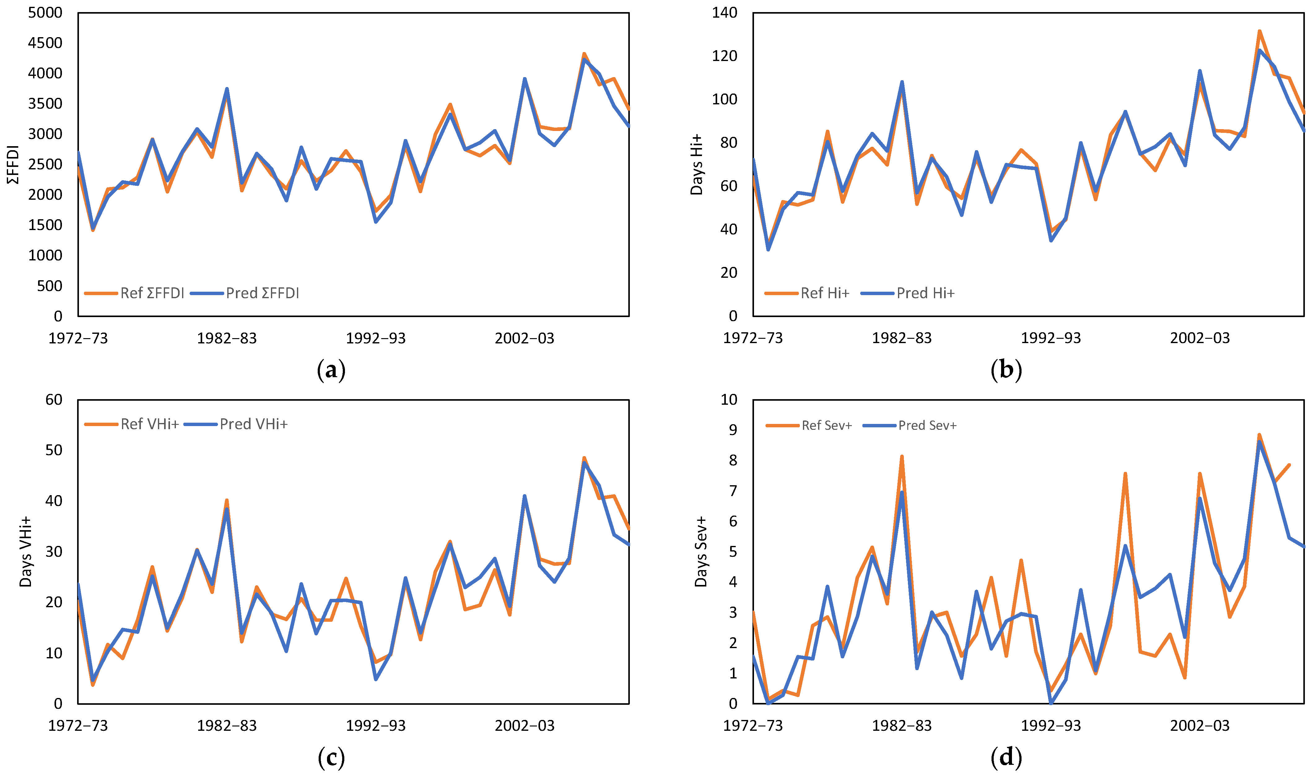
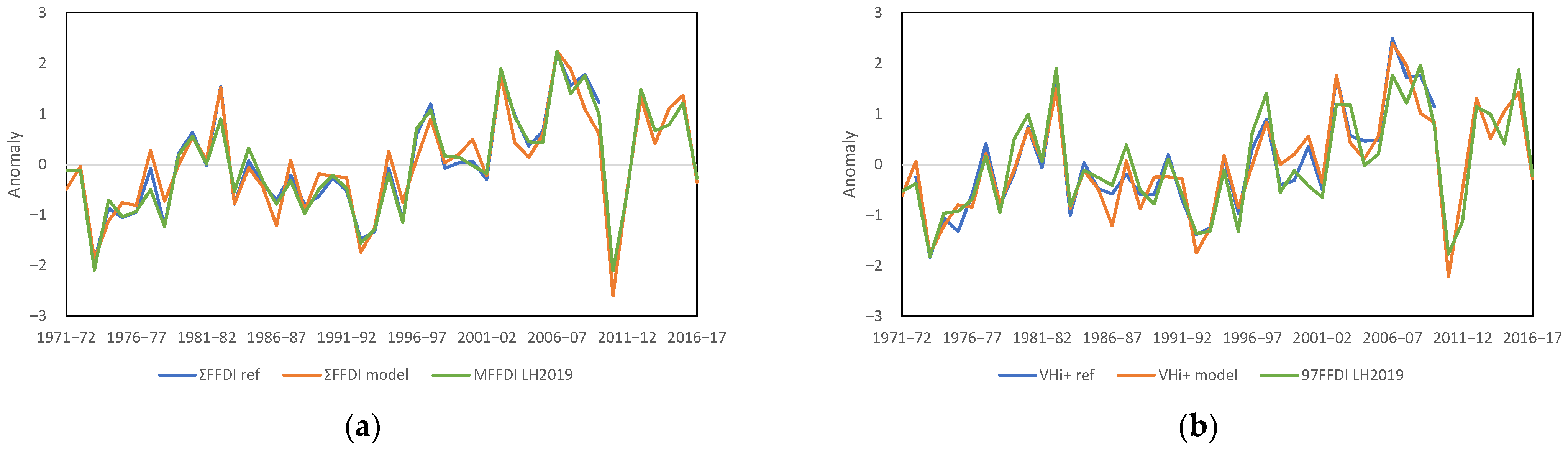
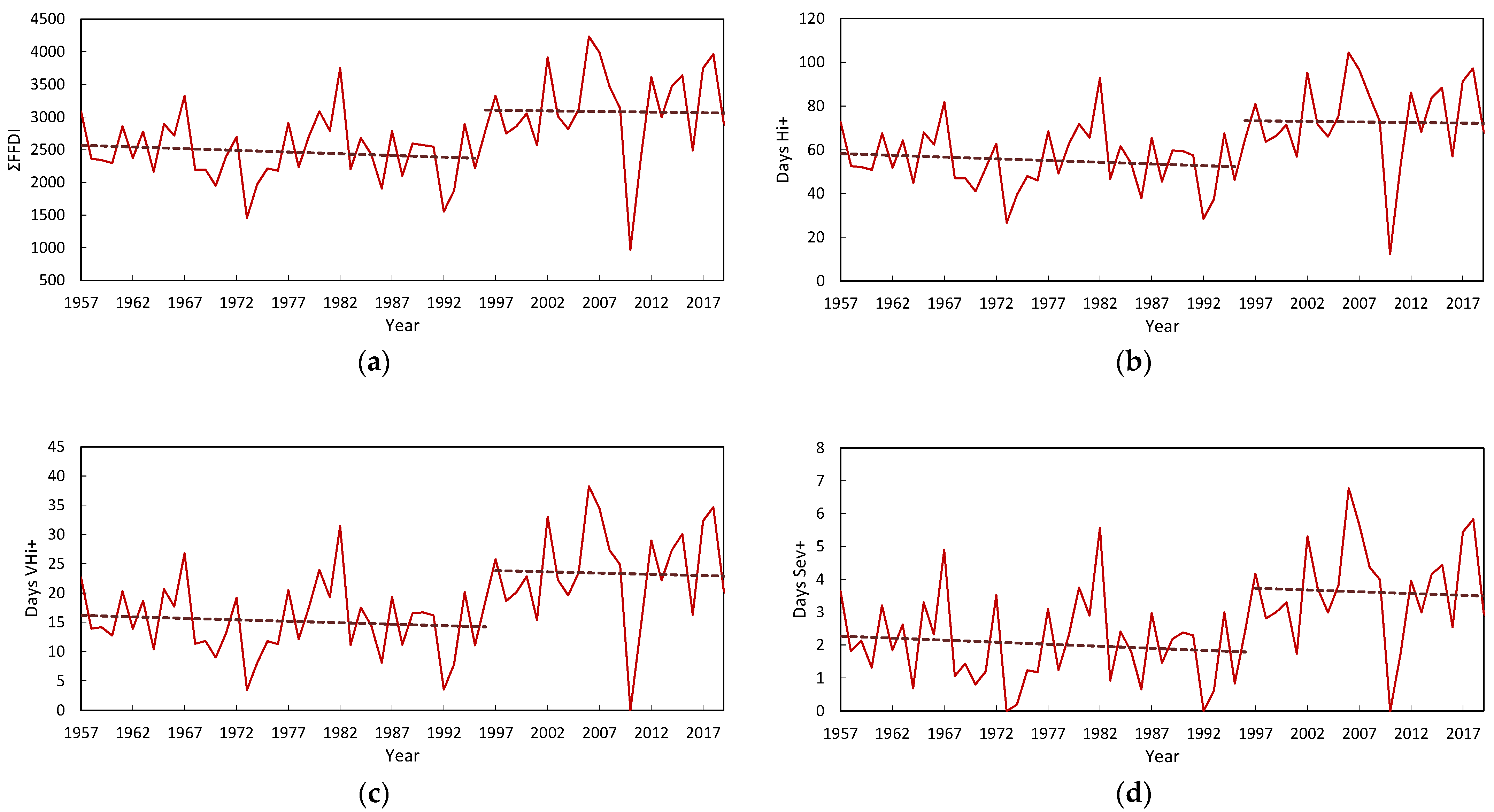
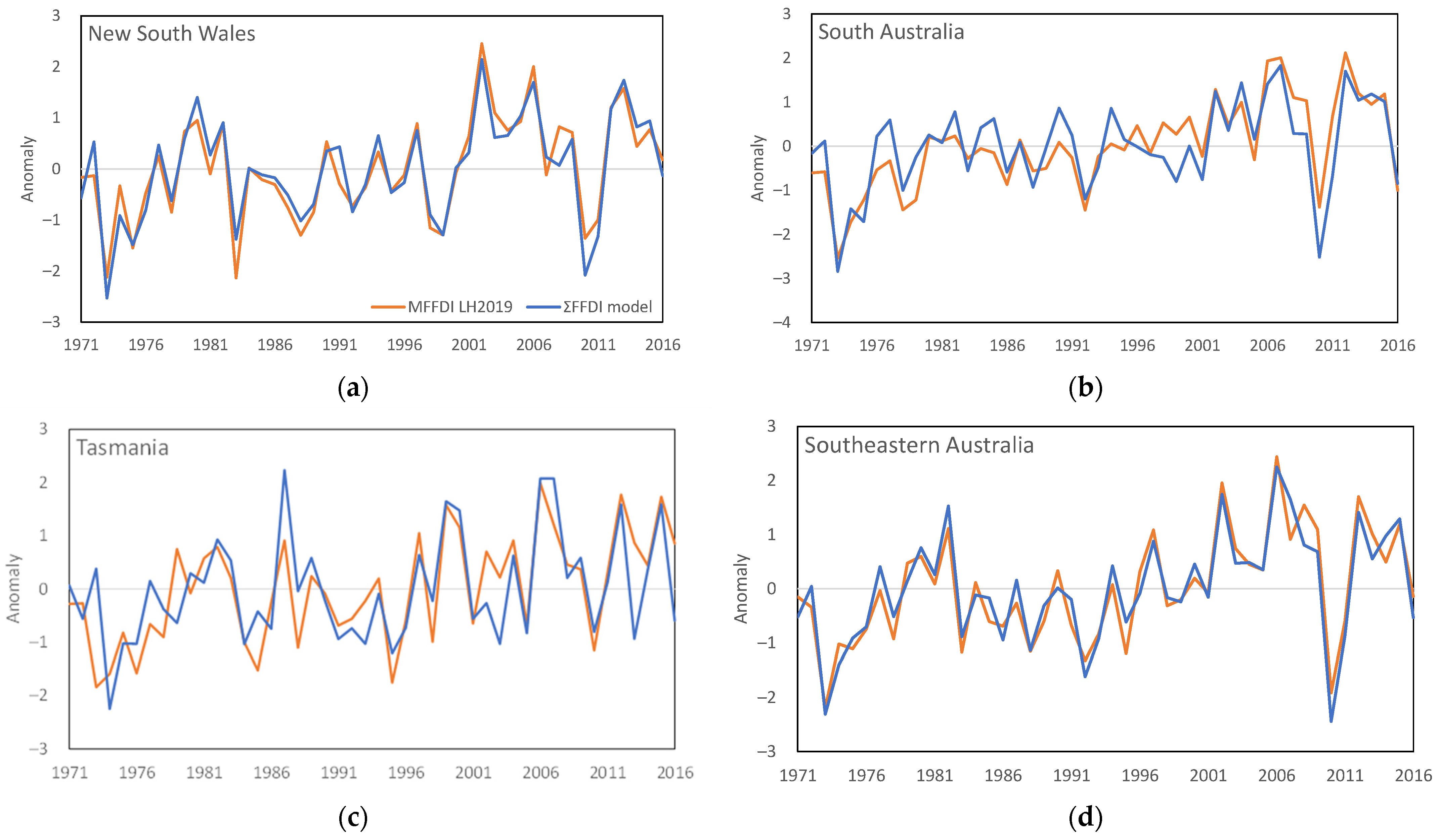
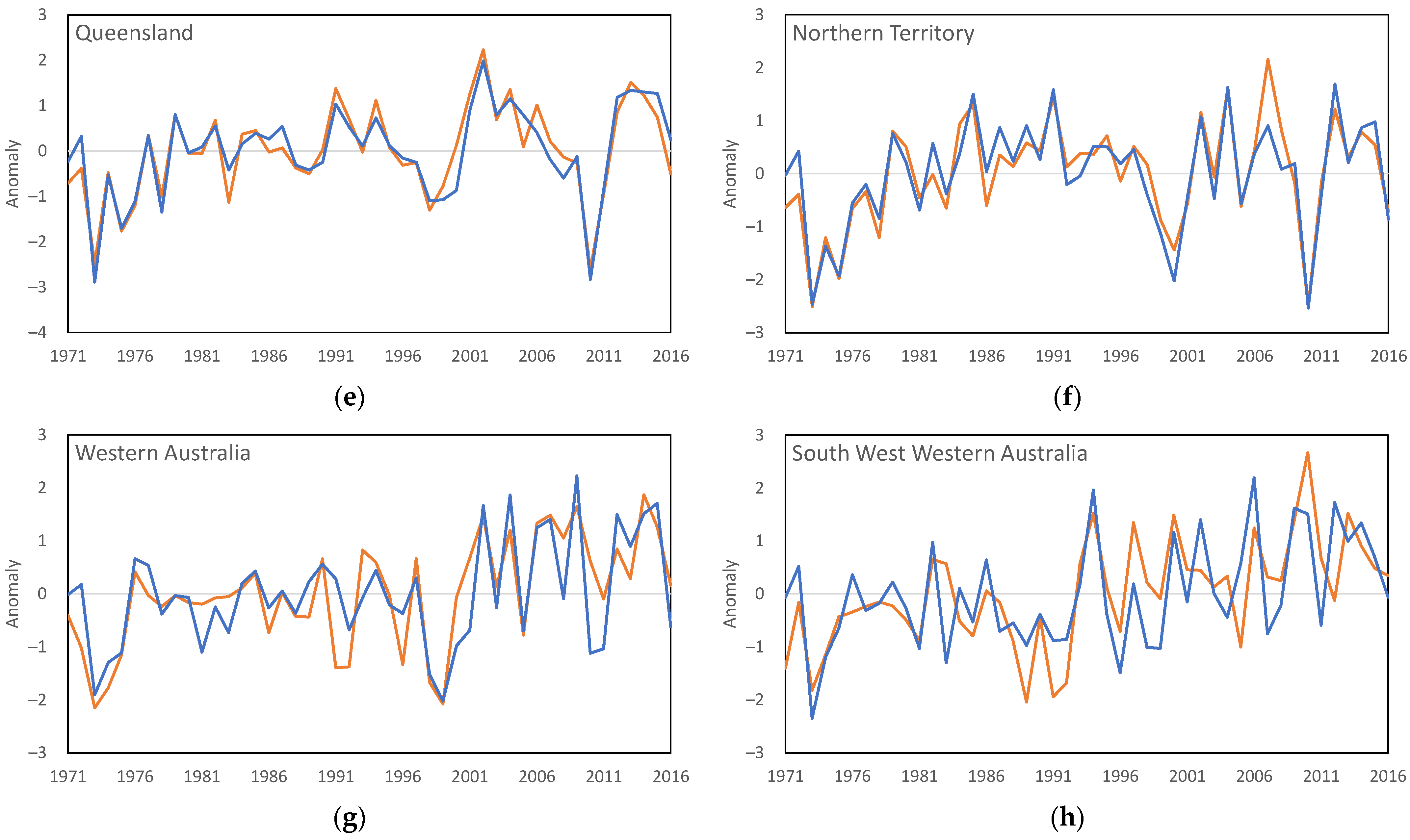
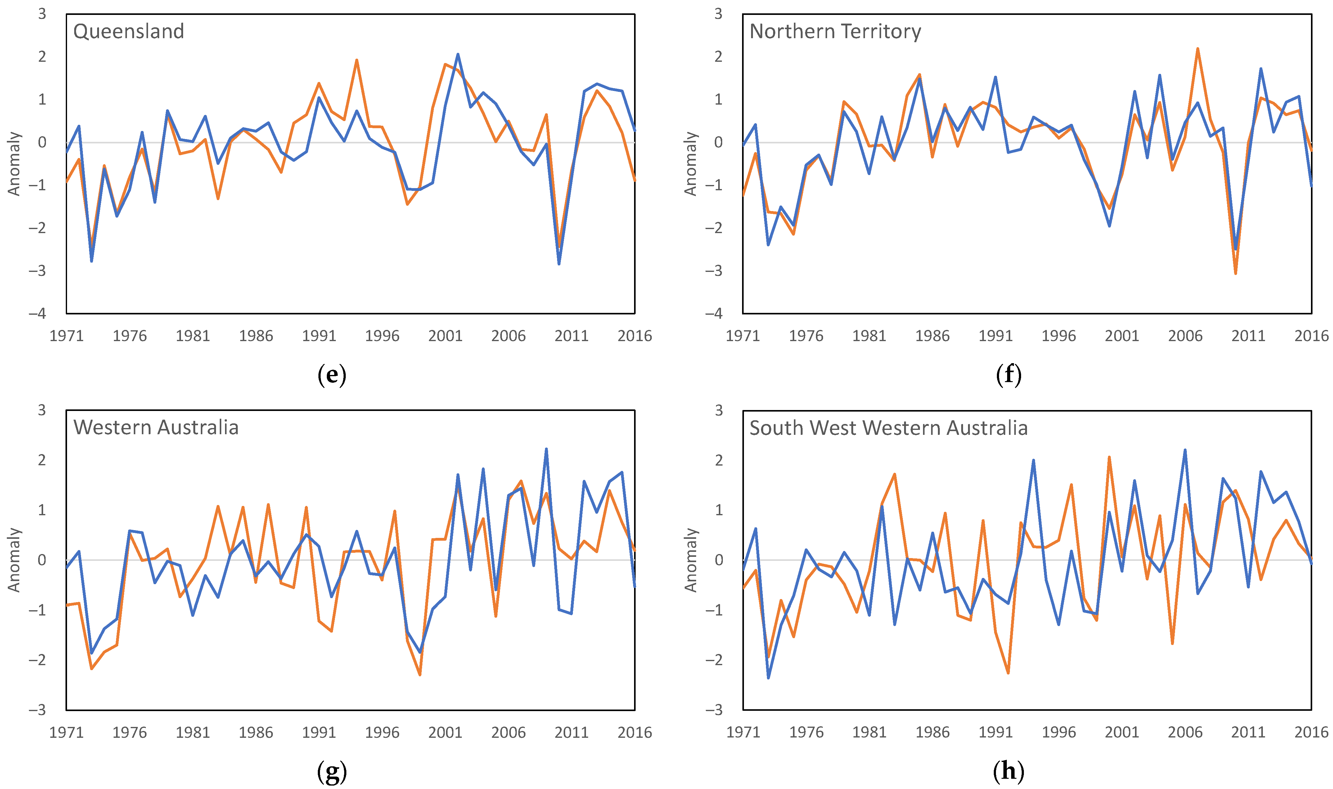
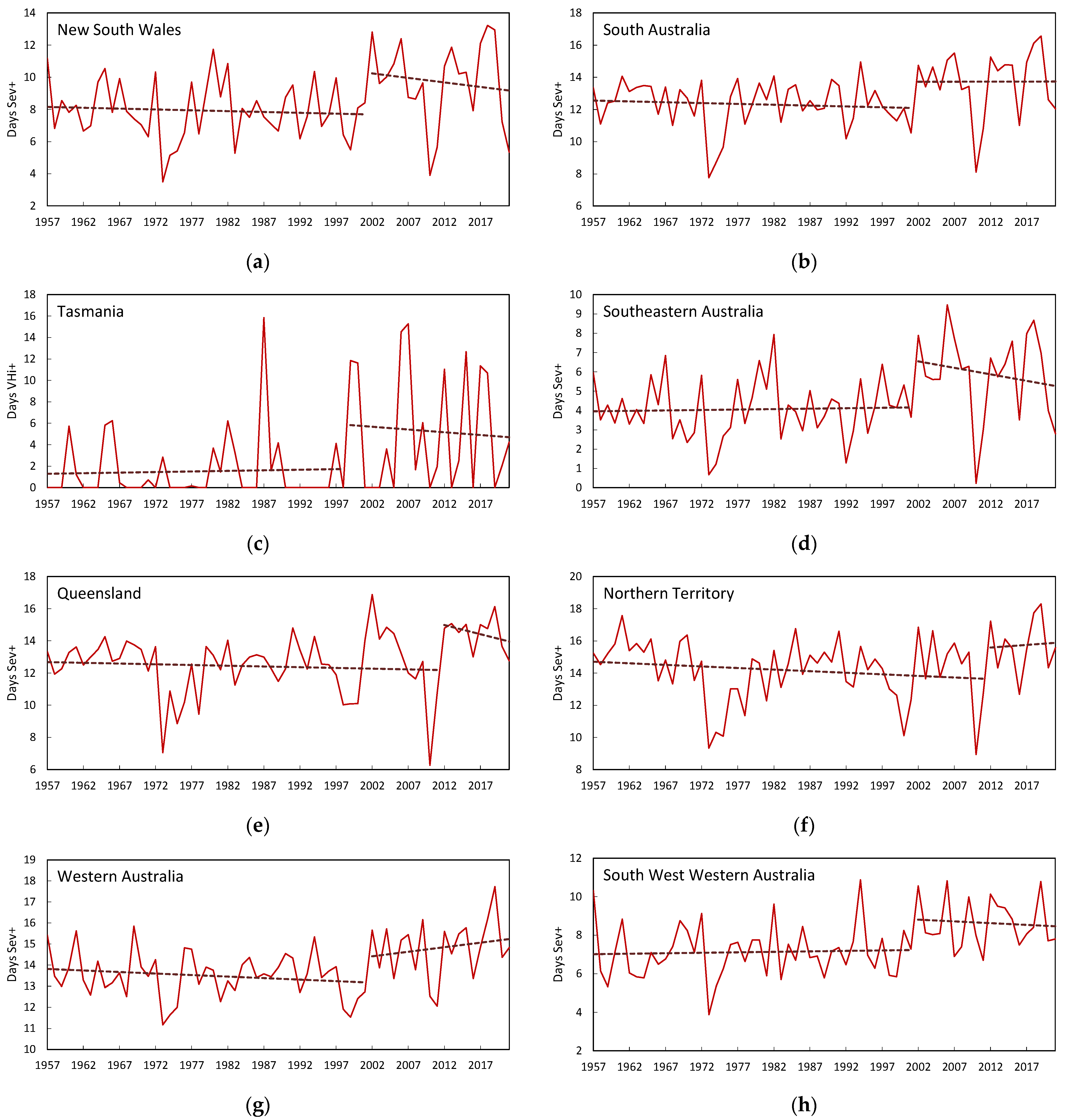
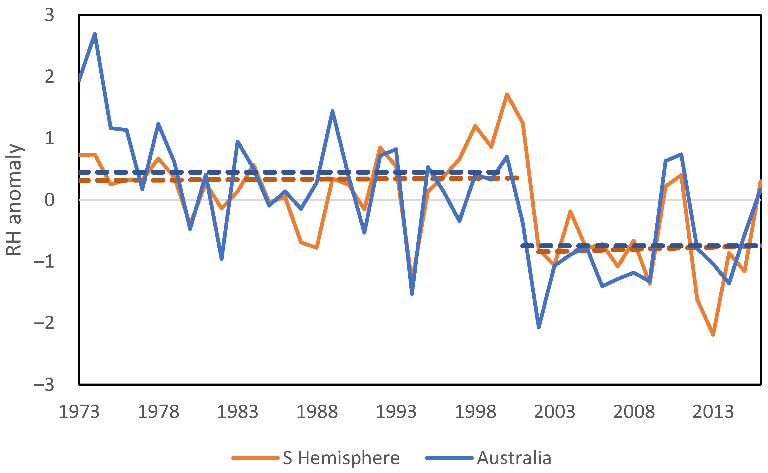
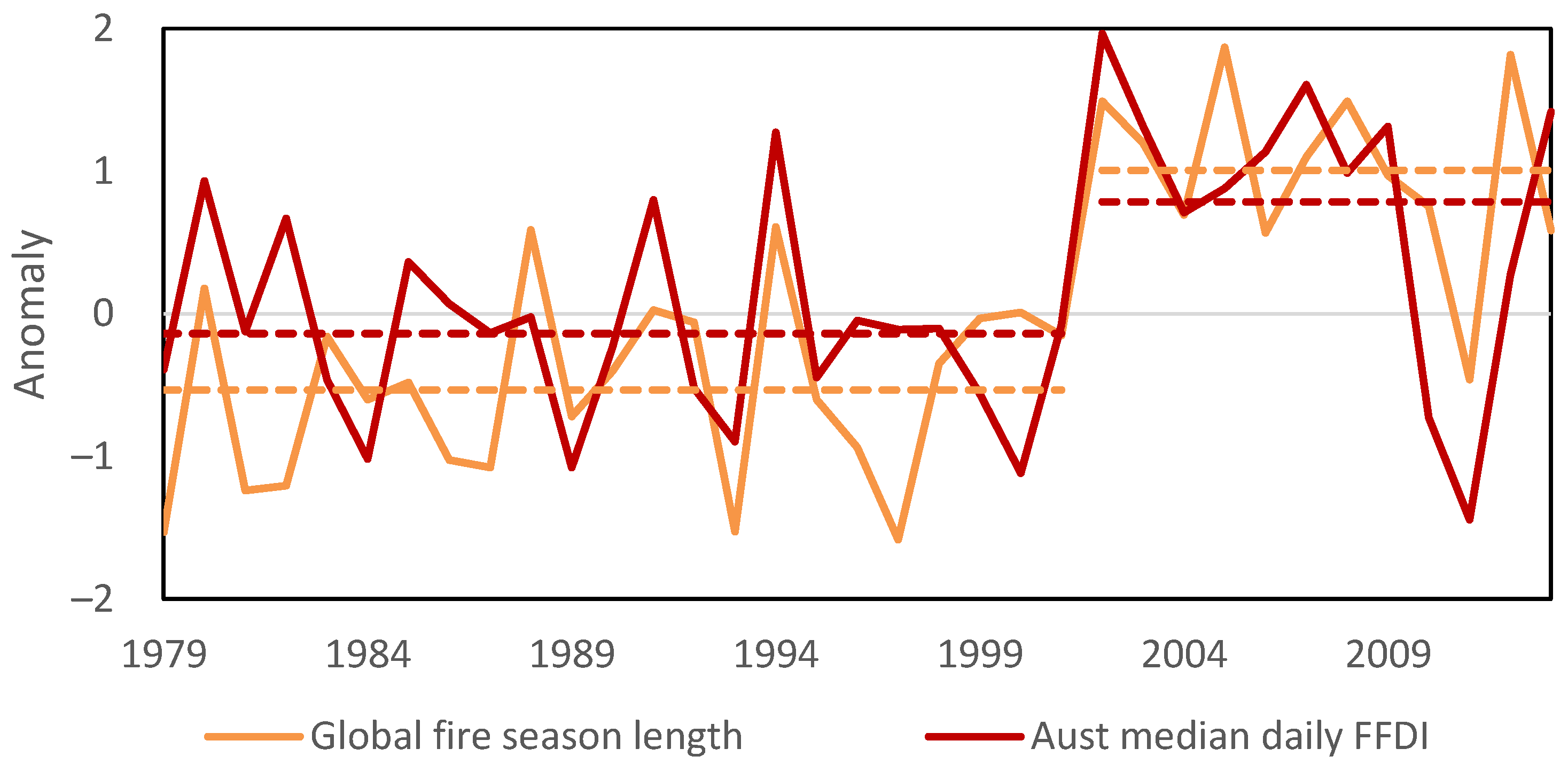
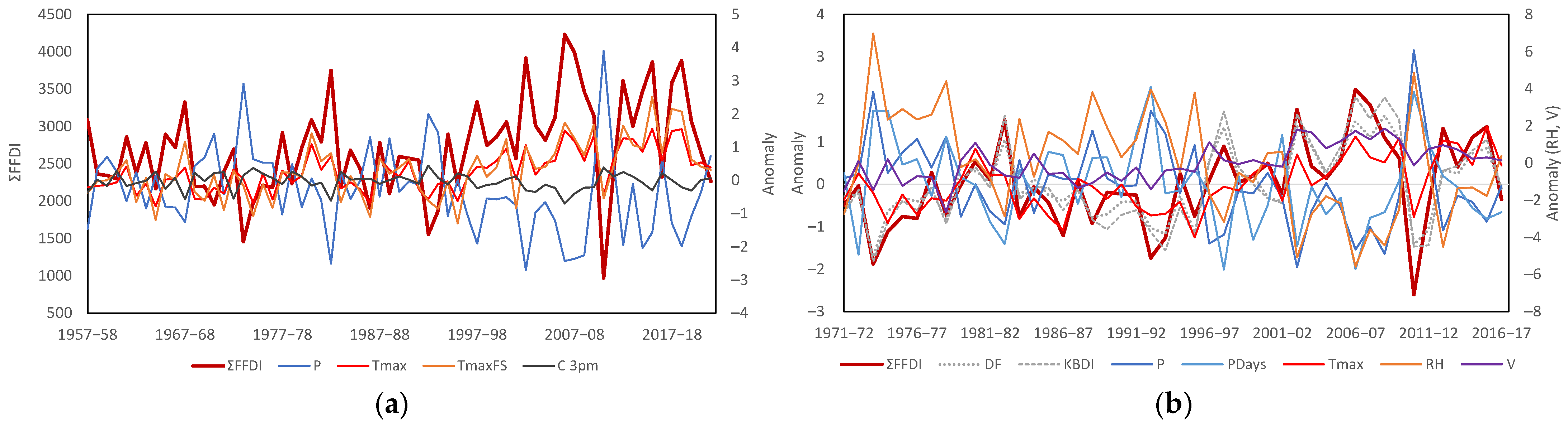
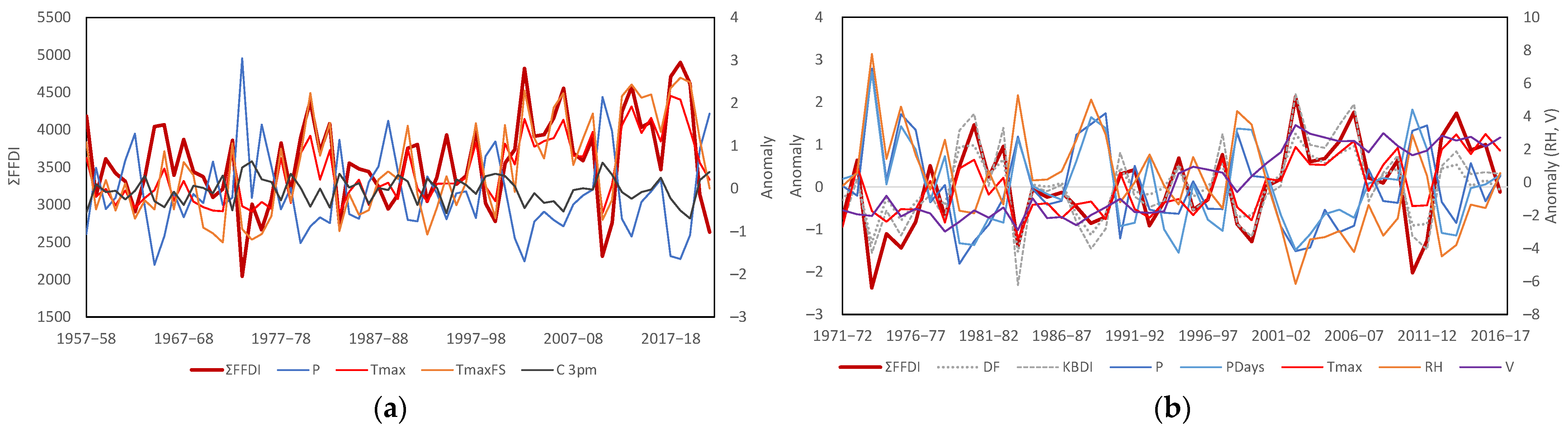
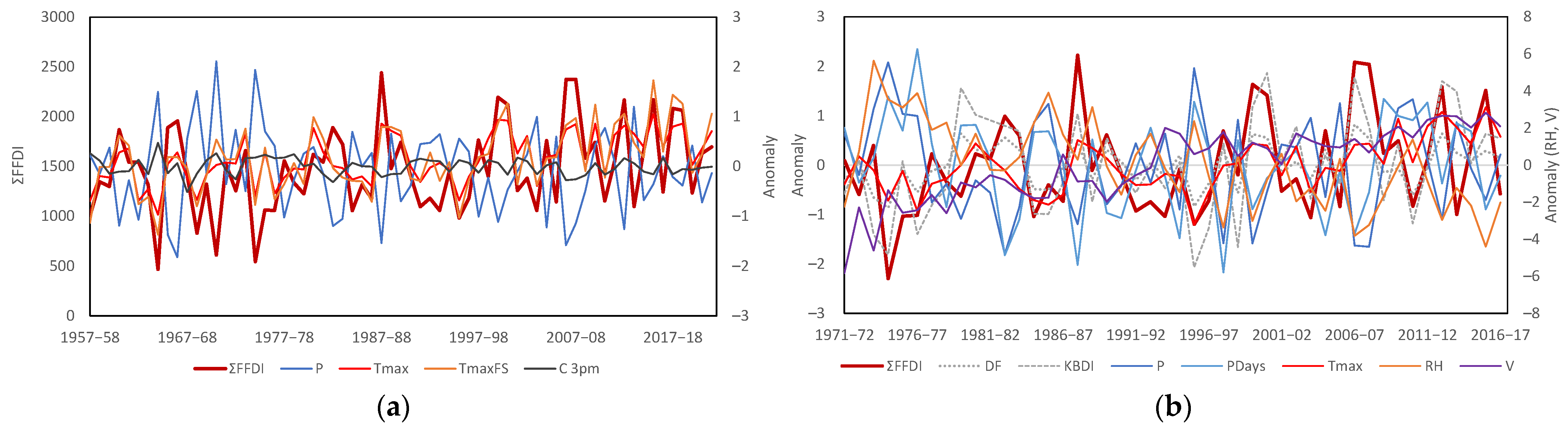
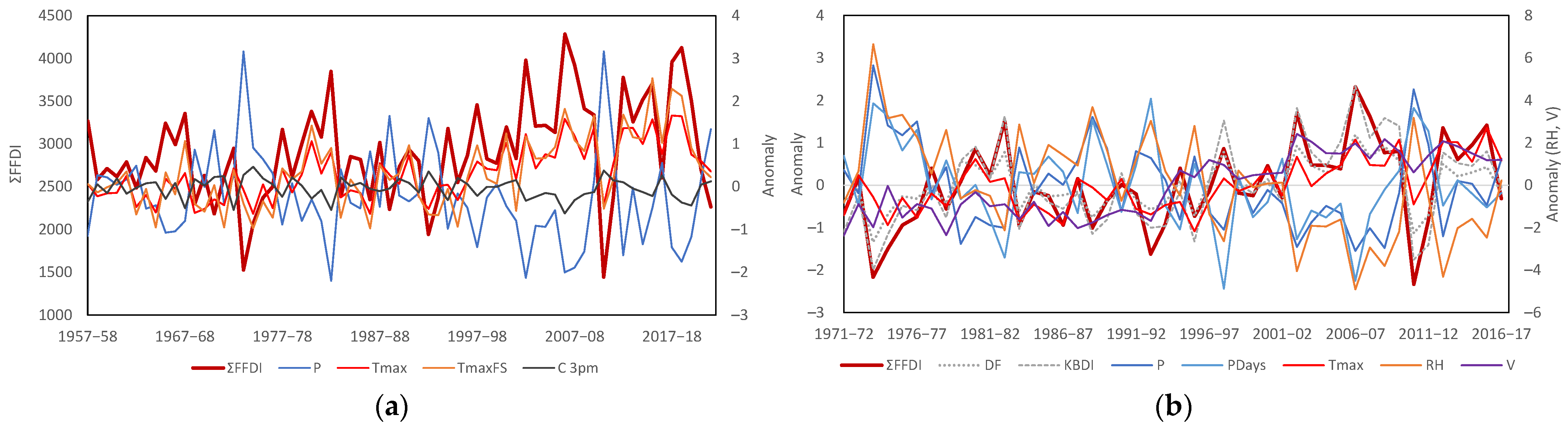
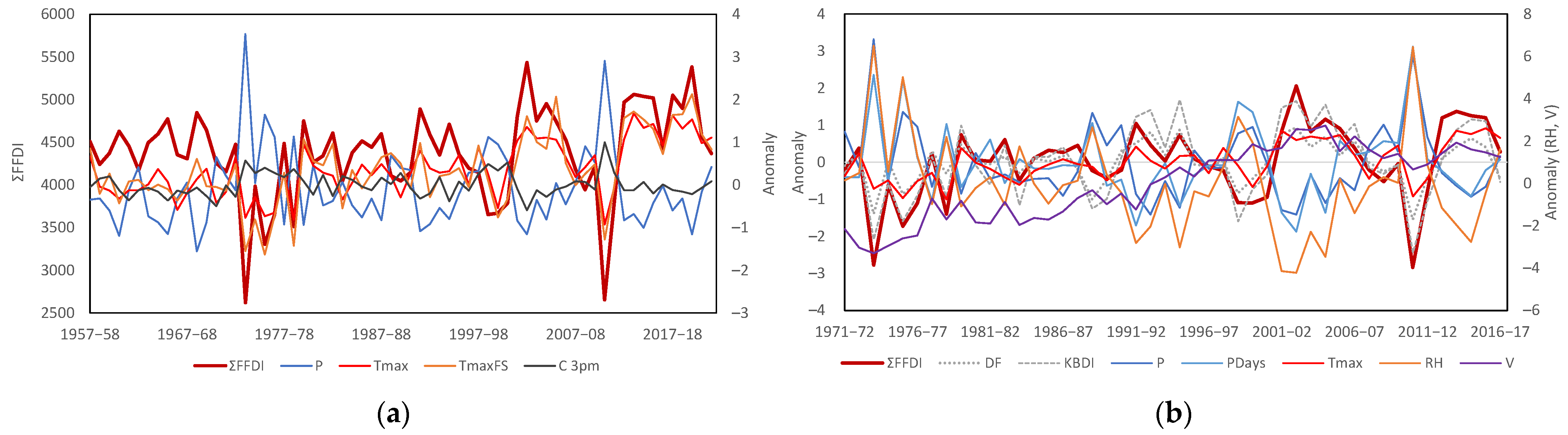
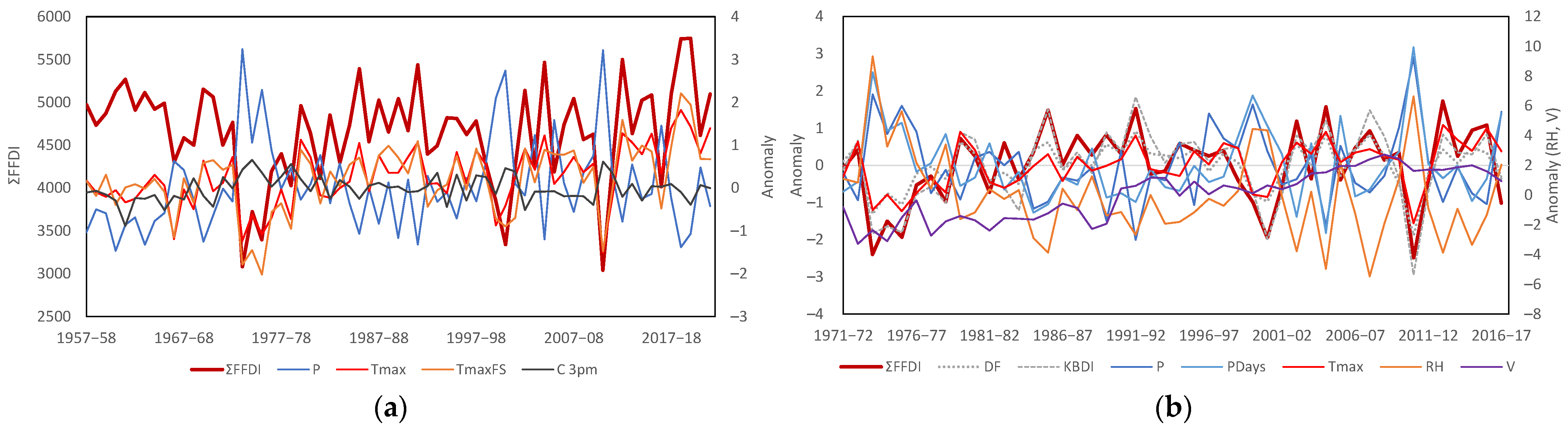
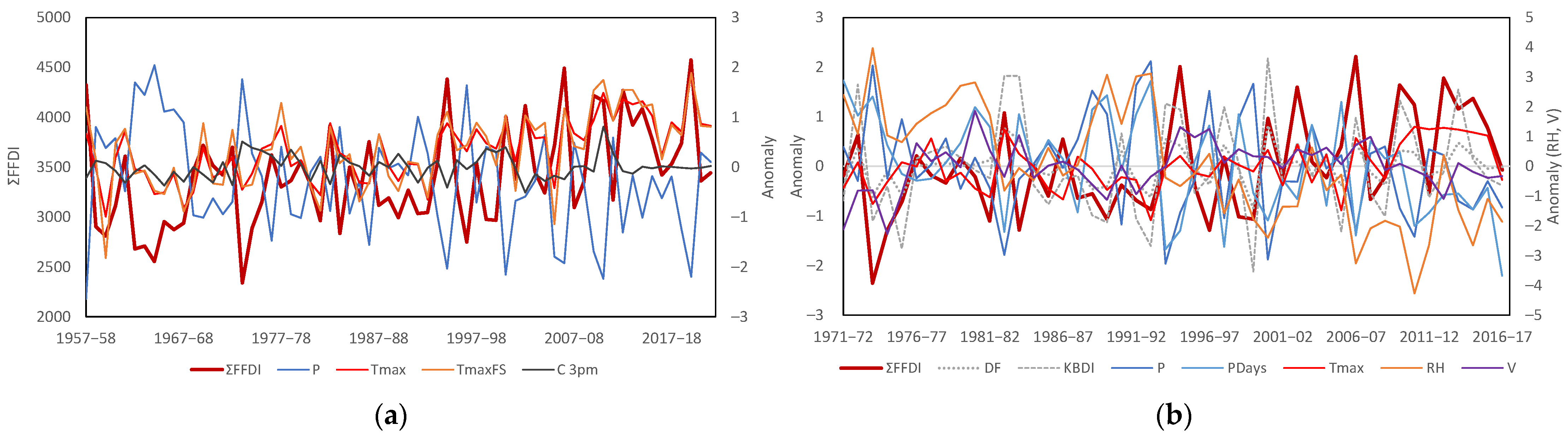
Table A1.
HQD regression model results for Victoria from 1972–2009 for predicted ΣFFDI, Days Hi+, Days VHi+, and Days Sev+, showing p values for each variable and main error statistics.
Table A1.
HQD regression model results for Victoria from 1972–2009 for predicted ΣFFDI, Days Hi+, Days VHi+, and Days Sev+, showing p values for each variable and main error statistics.
| Constants | p Values | |||||||
|---|---|---|---|---|---|---|---|---|
| Variables | ΣFFDI | Days Hi+ | Days VHi+ | Days Sev+ | ΣFFDI | Days Hi+ | Days VHi+ | Days Sev+ |
| Intercept | 1694.376 | 42.277 | 8.112 | 2.808 | 0.416 | 0.530 | 0.830 | 0.852 |
| P | −324.590 | −11.244 | −4.351 | −0.694 | 1.88 × 10⁻¹¹ | 3.37 × 10⁻¹² | 2.20 × 10⁻⁸ | 0.006 |
| TmaxFY | 127.254 | 3.925 | 2.288 | 0.631 | 0.064 | 0.077 | 0.068 | 0.199 |
| Tmax90 | 4.021 | 0.121 | 0.075 | 0.010 | 0.004 | 0.007 | 0.003 | 0.307 |
| C 3pm | −476.881 | −14.835 | −9.293 | −3.246 | 0.012 | 0.015 | 0.007 | 0.017 |
| Error | ||||||||
| Adj r2 | 0.93 | 0.93 | 0.90 | 0.70 | ||||
| SE | 178.5 | 5.78 | 3.26 | 0.13 |
For Table A2, each variable was omitted from the regression and the results tallied. The main outputs show the variation to the mean, shift size and timing, and standard deviation. They show different behavior within and between FFDIs as described in Section 3.1.3. FFDI results have also been allowed to fall below zero in response to the removal of TmaxFS as a sensitivity exercise.
Table A2.
Sensitivity testing using the bivariate test results for the HQD model for Victoria from 1957–2021 showing the result with each input variable removed for predicted ΣFFDI, Days Hi+, Days VHi+, and Days Sev+.
Table A2.
Sensitivity testing using the bivariate test results for the HQD model for Victoria from 1957–2021 showing the result with each input variable removed for predicted ΣFFDI, Days Hi+, Days VHi+, and Days Sev+.
| Variable–Omitted | Mean | Std. Dev. | Ti0 | Year | Shift | Mean Change (%) | Shift Change (%) | Std. Dev. Change (%) | p Value |
|---|---|---|---|---|---|---|---|---|---|
| ΣFFDI | 2715 | 636 | 14.5 | 1996–1997 | 616 | p < 0.01 | |||
| ΣFFDI–p | 2615 | 300 | 20.4 | 2002–2003 | 364 | –4% | –41% | –53% | p < 0.01 |
| ΣFFDI–TmaxFS | –364 | 556 | 12.3 | 1996–1997 | 495 | –113% | –20% | −12.5% | p < 0.01 |
| ΣFFDI–Tmax90 | 2644 | 554 | 11.0 | 1996–1997 | 463 | –3% | –25% | −12.9% | p < 0.05 |
| ΣFFDI–C3pm | 4943 | 558 | 15.9 | 1996–1997 | 563 | 82% | –8% | −12.2% | p < 0.01 |
| Days Hi+ | 62.4 | 18.4 | 14.7 | 1996–1997 | 17.8 | p < 0.01 | |||
| Days Hi+–P | 59.4 | 8.7 | 19.7 | 2002–2003 | 10.3 | –5% | –42% | –53% | p < 0.01 |
| Days Hi+–TmaxFS | −63.7 | 15.0 | 10.9 | 1996–1997 | 12.5 | –202% | −29.7% | –19% | p < 0.05 |
| Days Hi+–Tmax90 | 60.9 | 16.7 | 12.1 | 1996–1997 | 14.6 | –2% | –18% | –9% | p < 0.05 |
| Days Hi+–C3pm | 128.3 | 15.8 | 15.7 | 1996–1997 | 15.8 | 106% | –11% | –14% | p < 0.01 |
| Days VHi+ | 18.3 | 8.0 | 15.9 | 1997–1998 | 8.2 | p < 0.01 | |||
| Days VHi+–P | 17.2 | 4.5 | 19.6 | 2002–2003 | 5.3 | –6% | –35% | –44% | p < 0.01 |
| Days VHi+–TmaxFS | −31.5 | 6.8 | 12.3 | 1997–1998 | 6.0 | –272% | −26.1% | –15% | p < 0.01 |
| Days VHi+–Tmax90 | 17.4 | 7.0 | 11.6 | 1996–1997 | 6.1 | –5% | −25.9% | –12% | p < 0.05 |
| Days VHi+–C3pm | 54.5 | 6.8 | 17.2 | 1996–1997 | 7.1 | 197% | –13% | –15% | p < 0.01 |
| Days Sev+ | 2.6 | 1.6 | 15.6 | 1997–1998 | 1.6 | p < 0.01 | |||
| Days Sev+–P | 2.4 | 1.1 | 15.0 | 2002–2003 | 1.1 | –8% | –29% | –31% | p < 0.01 |
| Days Sev+–TmaxFS | −10.1 | 1.3 | 9.6 | 1997–1998 | 1.0 | –484% | –35% | –17% | p < 0.05 |
| Days Sev+–Tmax90 | 2.5 | 1.5 | 11.5 | 1997–1998 | 1.3 | –5% | –17% | –4% | p < 0.05 |
| Days Sev+–C3pm | 14.9 | 1.1 | 17.7 | 1996–1997 | 1.2 | 466% | –23% | –27% | p < 0.01 |
Table A3 shows the results for changes that are closer to what might be experienced by observed changes. The variables were each varied by 10%, whereas the standard deviations for P from 1957–2021 are 15%, for TmaxFS 3%, Tmax90 is almost 200% due to the highly nonlinear time series, and C3pm is 5%.
Table A3.
Sensitivity testing using the bivariate test results for the HQD model for Victoria from 1957–2021 showing the result with each input variable increased by 10% for predicted ΣFFDI, Days Hi+, Days VHi+, and Days Sev+.
Table A3.
Sensitivity testing using the bivariate test results for the HQD model for Victoria from 1957–2021 showing the result with each input variable increased by 10% for predicted ΣFFDI, Days Hi+, Days VHi+, and Days Sev+.
| Variable–Omitted | Mean | Std. Dev. | Ti0 | Year | Shift | Mean Change (%) | Shift Change (%) | Std. Dev. Change (%) | p Value |
|---|---|---|---|---|---|---|---|---|---|
| ΣFFDI | 2715 | 636 | 14.5 | 1995 | 616 | p < 0.01 | |||
| ΣFFDI 0.1P | 2725 | 674 | 14.4 | 1995 | 644 | 0.4% | 4.6% | 6% | p < 0.01 |
| ΣFFDI 0.1TmaxFS | 3022 | 644 | 14.6 | 1995 | 635 | 11% | 3.1% | 1.3% | p < 0.01 |
| ΣFFDI 0.1Tmax90 | 2722 | 645 | 14.8 | 1996 | 634 | 0.3% | 3.1% | 1.5% | p < 0.01 |
| ΣFFDI 0.1C3pm | 2492 | 644 | 14.4 | 1995 | 622 | −8% | 1.1% | 1.3% | p < 0.01 |
| Days Hi+ | 62.4 | 18.4 | 14.7 | 1995 | 17.8 | p < 0.01 | |||
| Days Hi+0.1P | 62.5 | 19.2 | 13.9 | 1995 | 18.1 | 0.2% | 1.8% | 4% | p < 0.01 |
| Days Hi+0.1TmaxFS | 74.8 | 18.5 | 14.4 | 1995 | 18.0 | 20% | 1.1% | 0.5% | p < 0.01 |
| Days Hi+0.1Tmax90 | 62.3 | 18.3 | 14.5 | 1995 | 17.7 | −0.1% | −0.7% | −0.5% | p < 0.01 |
| Days Hi+0.1C3pm | 55.6 | 18.4 | 14.0 | 1995 | 17.5 | −11% | −1.5% | 0.03% | p < 0.01 |
| Days VHi+ | 18.3 | 8.0 | 15.9 | 1996 | 8.2 | p < 0.01 | |||
| Days VHi+0.1P | 18.4 | 8.5 | 14.9 | 1996 | 8.3 | 0.4% | 1.9% | 6% | p < 0.01 |
| Days VHi+0.1TmaxFS | 23.3 | 8.2 | 15.4 | 1996 | 8.2 | 27% | 0.5% | 3.1% | p < 0.01 |
| Days VHi+0.1Tmax90 | 18.4 | 8.2 | 15.5 | 1996 | 8.2 | 0.3% | 0.8% | 2.9% | p < 0.01 |
| Days VHi+0.1C3pm | 14.7 | 8.2 | 14.9 | 1996 | 8.1 | −20% | −0.9% | 3.1% | p < 0.01 |
| Days Sev+ | 2.6 | 1.6 | 15.6 | 1996 | 1.6 | p < 0.01 | |||
| Days Sev+0.1P | 2.6 | 1.7 | 13.5 | 1996 | 1.6 | 0% | −0.36% | 8% | p < 0.01 |
| Days Sev+0.1TmaxFS | 3.9 | 1.7 | 13.9 | 1996 | 1.6 | 47% | −0.01% | 6% | p < 0.01 |
| Days Sev+0.1Tmax90 | 2.6 | 1.6 | 13.9 | 1996 | 1.6 | −0.7% | −1.6% | 5% | p < 0.01 |
| Days Sev+0.1C3pm | 1.4 | 1.7 | 13.2 | 1996 | 1.6 | −48% | −0.38% | 7% | p < 0.01 |
Appendix B. Nonlinear Attribution Test Results
This Appendix contains results for the paired bivariate tests. Due to their novelty, we have included a comprehensive set of results for each region tested. For each table, the upper part of each panel showing single variables was tested against a random reference time series, which is the standard way of assessing regime shifts. The lower part contains paired shifts where one is the reference and the other is the test, and these are mirrored. The following points will help interpret those results:
- Two time series containing a common shift will show no shift when paired if those shifts are proportional. For example, pairing the different measures of FFDIs for a single region shows no regime change when paired or mirrored (p > 0.10). This may denote a common origin for both variables or direct cause-and-effect where one forces the other (i.e., full attribution).
- Partial attribution may be the case when a pair has similar regime shifts and one shows no shift when paired in one direction, but when mirrored only part of the original shift can be attributed. RH shows this for many regions: the FFDI shows no shift against RH, but RH against the FFDI reproduces only part of its regime change. For example, for Victoria, RH shifted by −3.2 in 1996–1997 which is compatible with the FFDI, but in reverse it showed a relative shift of −1.4 in the same year, so only −1.8 can be accounted for.
- Shifts due to an independent process may show conformity in one direction but none when mirrored. This is consistent with windspeed, which shows a potential attribution of 0.1−0.3 m s−1 for regime shifts in the early to mid-1990s that are in excess of 2.0 m s−1, where we know measurement methods changed over at that time.
- When two variables with shifts in common show no shift at that time, but relative shifts at other times, they are conformal for the regime shift but reflect the presence of other processes that will need a separate interpretation.
- Other results can show nonlinear responses or shifts due to an independent process not directly related to a change in fire climates, including inhomogeneities. Climate variability may also be a factor in short sequences.
Appendix B.1. Victoria
Table A4.
Bivariate test results for the HQD and LH2019 FFDI record for Victoria covering predicted ΣFFDI and Days Sev+ and input variables, along with selected mirrored pairs showing shifts relative to each in variable/reference format.
Table A4.
Bivariate test results for the HQD and LH2019 FFDI record for Victoria covering predicted ΣFFDI and Days Sev+ and input variables, along with selected mirrored pairs showing shifts relative to each in variable/reference format.
| Variable | Average | Std. Dev. | Ti0 | Year | Change | p Value | Variable | Average | Std. Dev. | Ti0 | Year | Change | p Value |
|---|---|---|---|---|---|---|---|---|---|---|---|---|---|
| 1957–2021 HQD inputs | Notes | ||||||||||||
| ΣFFDI | 2715 | 636 | 14.5 | 1996–1997 | 616 | p < 0.01 | ΣFFDI shifted up in 1996–1997, although the inputs show different timing; up relative to P in 2006–2007 and to TmaxFS in 2009–2010. This is due to a sequence of wet and dry years following the Millennium drought. Suppression of Tmax by P in wet years had little effect on mean FFDI, which became far more variable. ΣFFDI shifted up in 1996–1997 relative to cloud, showing the latter had a small influence (175 of 616). Tmax90 also had a limited influence. | ||||||
| Days Sev+ | 2.6 | 1.6 | 15.6 | 1997–1998 | 1.6 | p < 0.01 | |||||||
| P | 641 | 94 | 8.7 | 1994–1995 | –68 | p < 0.10 | |||||||
| TmaxFS | 24.2 | 0.84 | 22 | 2002–2003 | 1.06 | p < 0.01 | |||||||
| C 3pm | 4.67 | 0.25 | 3.6 | 1997–1998 | −0.12 | ||||||||
| Tmax90 | 17.6 | 34.8 | 23.9 | 2006–2007 | 49 | p < 0.01 | |||||||
| ΣFFDI/P | 2715 | 636 | 16.2 | 2006–2007 | 302 | p < 0.01 | P/ΣFFDI | 641 | 94 | 10.6 | 2006–2007 | 38 | p < 0.05 |
| ΣFFDI/Tmax | 2715 | 636 | 7.1 | 2009–2010 | –371 | Tmax/ΣFFDI | 20.2 | 0.6 | 21.9 | 2009–2010 | 0.6 | p < 0.01 | |
| ΣFFDI/TmaxFS | 2715 | 636 | 6.2 | 2009–2010 | –383 | TmaxFS/ΣFFDI | 24.2 | 0.8 | 18.7 | 2009–2010 | 0.7 | p < 0.01 | |
| ΣFFDI/C 3pm | 2715 | 636 | 14.2 | 1996–1997 | 441 | p < 0.01 | C 3pm/ΣFFDI | 4.7 | 0.2 | 7 | 2012–2013 | 0.2 | |
| ΣFFDI/Tmax90 | 2715 | 636 | 2.8 | 1994–1995 | 231 | Tmax90/ΣFFDI | 17.6 | 34.8 | 17.5 | 2006–2007 | 34.3 | p < 0.01 | |
| Tmax/P | 20.2 | 0.6 | 24.1 | 1999–2000 | 0.7 | p < 0.01 | P/Tmax | 641 | 94 | 7 | 2009–2010 | 77 | |
| TmaxFS/P | 24.2 | 0.8 | 20.6 | 2004–2005 | 0.9 | p < 0.01 | P/TmaxFS | 641 | 94 | 7.5 | 2009–2010 | 76 | |
| 1971–2016 LH2019 inputs | Notes | ||||||||||||
| DF | 6.9 | 0.8 | 12.7 | 1996–1997 | 0.8 | p < 0.01 | The direct inputs to FFDIs all contribute to the regime shift. DF and KBDI both had a positive influence. P had a higher influence than rain days. For RH, half of the recorded shift (−1.4 of −3.2) had a strong influence, suggesting the possibility of both a shift and inhomogeneity. The same may be true of windspeed. Days Sev+ shows similar patterns to ΣFFDI. The occluded warmer/wetter events from 2010 onwards also had little effect on FFDI. | ||||||
| KBDI | 60.8 | 21.7 | 13.5 | 1996–1997 | 23.6 | p < 0.01 | |||||||
| P | 476.2 | 101.9 | 7.3 | 1996–1997 | −82.8 | ||||||||
| Pdays | 126.7 | 10.7 | 4.6 | 1993–1994 | −6.8 | ||||||||
| RH | 50.7 | 2.8 | 15.2 | 1996–1997 | −3.2 | p < 0.01 | |||||||
| Tmax | 20.9 | 0.6 | 18.3 | 1999–2000 | 0.8 | p < 0.01 | |||||||
| V | 20.3 | 1 | 21.4 | 1996–1997 | 1.4 | p < 0.01 | |||||||
| ΣFFDI/DF | 2725 | 674 | 3.9 | 2011–2012 | 291 | DF/ΣFFDI | 6.9 | 0.8 | 2.9 | 1996–1997 | 0.2 | ||
| ΣFFDI/KBDI | 2725 | 674 | 4.1 | 2011–2012 | 311 | KBDI/ΣFFDI | 60.8 | 21.7 | 4 | 1996–1997 | 7.6 | ||
| ΣFFDI/P | 2725 | 674 | 7.4 | 1999–2000 | 301 | P/ΣFFDI | 476.2 | 101.9 | 3.3 | 2006–2007 | 35.2 | ||
| ΣFFDI/Pdays | 2725 | 674 | 10.2 | 1999–2000 | 432 | p < 0.05 | Pdays/ΣFFDI | 126.7 | 10.7 | 4 | 1973–1974 | 10.1 | |
| ΣFFDI/RH | 2732 | 680 | 3.1 | 1983–1984 | –213 | RH/ΣFFDI | 50.7 | 2.8 | 9.3 | 1996–1997 | −1.4 | p < 0.05 | |
| ΣFFDI/Tmax | 2725 | 674 | 8 | 2009–2010 | –553 | p < 0.10 | Tmax/ΣFFDI | 20.9 | 0.6 | 15.1 | 2009–2010 | 0.6 | p < 0.01 |
| ΣFFDI/V | 2725 | 674 | 2.1 | 2012–2013 | 374 | V/ΣFFDI | 20.3 | 1 | 14.9 | 2002–2003 | 1.1 | p < 0.01 | |
| Sev+/DF | 2.6 | 1.6 | 2.7 | 1987–1988 | 0.4 | DF/Sev+ | 6.9 | 0.8 | 2 | 1996–1997 | 0.2 | ||
| Sev+/KBDI | 2.6 | 1.6 | 2.5 | 1987–1988 | 0.4 | KBDI/Sev+ | 60.8 | 21.7 | 2.9 | 1996–1997 | 6.2 | ||
| Sev+/P | 2.6 | 1.6 | 9.1 | 2002–2003 | 1 | p < 0.05 | P/Sev+ | 476.2 | 101.9 | 2.6 | 2004–2005 | 36.9 | |
| Sev+/Pdays | 2.6 | 1.6 | 13.5 | 2001–2002 | 1.1 | p < 0.01 | Pdays/Sev+ | 126.7 | 10.7 | 6.1 | 2001–2002 | 5.6 | |
| Sev+/RH | 2.7 | 1.6 | 3.2 | 1983–1984 | −0.5 | RH/Sev+ | 50.7 | 2.8 | 7.8 | 1996–1997 | −1.4 | p < 0.10 | |
| Sev+/Tmax | 2.6 | 1.6 | 8.3 | 2009–2010 | −1.3 | p < 0.10 | Tmax/Sev+ | 20.9 | 0.6 | 15.3 | 2009–2010 | 0.6 | p < 0.01 |
| Sev+/V | 2.6 | 1.6 | 2.1 | 1977–1978 | 0.8 | V/Sev+ | 20.3 | 1 | 13.6 | 1996–1997 | 1 | p < 0.01 | |
Figure A1.
Comparison of predicted ΣFFDI for Victoria with inputs from (a) the BoM high quality data for 1957–2021 fire years; (b) the LH2019 data for the 1971–2016 fire years.
Figure A1.
Comparison of predicted ΣFFDI for Victoria with inputs from (a) the BoM high quality data for 1957–2021 fire years; (b) the LH2019 data for the 1971–2016 fire years.

Appendix B.2. New South Wales
Table A5.
Bivariate test results for the HQD and LH2019 FFDI record for New South Wales covering predicted ΣFFDI and Days Sev+ and input variables, along with selected mirrored pairs showing shifts relative to each in variable/reference format.
Table A5.
Bivariate test results for the HQD and LH2019 FFDI record for New South Wales covering predicted ΣFFDI and Days Sev+ and input variables, along with selected mirrored pairs showing shifts relative to each in variable/reference format.
| Variable | Average | Std. Dev. | Ti0 | Year | Change | p Value | Variable | Average | Std. Dev. | Ti0 | Year | Change | p Value |
|---|---|---|---|---|---|---|---|---|---|---|---|---|---|
| 1957–2021 HQD inputs | Notes | ||||||||||||
| ΣFFDI | 3574 | 601 | 8.9 | 2001–2002 | 474 | p < 0.10 | ΣFFDI shifted up in 2001–2002 and Days Sev+ the following year. The timing of Tmax showed increases coinciding with this. TmaxFS increased further after 2009. P is enhanced after 2005, mainly through wet years being wetter affecting FFDI variability but not the mean. ΣFFDI shifted up in 1996–1996 relative to cloud, showing the latter had a small influence (95 of 474). Tmax90 also had a limited influence. | ||||||
| Days Sev+ | 6.9 | 1.8 | 8.4 | 2002–2003 | 1.4 | p < 0.10 | |||||||
| P | 542 | 118 | 4.9 | 2019–2020 | 188 | ||||||||
| TmaxFS | 28.2 | 1.12 | 23.3 | 2002–2003 | 1.4 | p < 0.01 | |||||||
| C 3pm | 3.8 | 0.3 | 2.8 | 1957–1958 | 0.5 | ||||||||
| Tmax90 | 17.2 | 31.0 | 28.8 | 2002–2003 | 45 | p < 0.01 | |||||||
| ΣFFDI/P | 3574 | 601 | 21.9 | 2002–2003 | 364 | p < 0.01 | P/ΣFFDI | 541.6 | 118.2 | 16.0 | 2004–2005 | 65.6 | p < 0.01 |
| ΣFFDI/Tmax | 3574 | 601 | 14.8 | 1995–1996 | –429 | p < 0.01 | Tmax/ΣFFDI | 24.3 | 0.7 | 32.0 | 1997–1998 | 0.7 | p < 0.01 |
| ΣFFDI/TmaxFS | 3574 | 601 | 9.4 | 2008–2009 | –371 | p < 0.05 | TmaxFS/ΣFFDI | 28.2 | 1.1 | 21.4 | 1997–1998 | 0.8 | p < 0.01 |
| ΣFFDI/C 3pm | 3574 | 601 | 15.0 | 2000–2001 | 379 | p < 0.01 | C 3pm/ΣFFDI | 3.8 | 0.3 | 9.8 | 1995–1996 | 0.2 | p < 0.05 |
| ΣFFDI/Tmax90 | 3574 | 601 | 8.8 | 2009–2010 | –471 | p < 0.10 | Tmax90/ΣFFDI | 17.6 | 34.8 | 17.5 | 2006–2007 | 34.3 | p < 0.01 |
| Tmax/P | 24.3 | 0.7 | 34.7 | 2000–2001 | 1.0 | p < 0.01 | P/Tmax | 541.6 | 118.2 | 13.7 | 2004–2005 | 124.8 | p < 0.01 |
| TmaxFS/P | 28.2 | 1.1 | 27.2 | 2002–2003 | 1.3 | p < 0.01 | P/TmaxFS | 541.6 | 118.2 | 10.7 | 2008–2009 | 112.5 | p < 0.05 |
| 1971–2016 LH2019 inputs | Notes | ||||||||||||
| DF | 6.3 | 0.6 | 5.1 | 2001–2002 | 0.4 | The direct inputs to FFDIs all contributed to the regime shift. DF and KBDI both had a positive minor influence. P had limited influence after 1978. For RH, half of the recorded shift (−1.8 of −3.5) had a strong influence, suggesting the possibility of both a shift and inhomogeneity. Windspeed suggests a large shift in 1994–1995 relative to the FFDI. Days Sev+ shows similar patterns to ΣFFDI. The occluded warmer/wetter events from 2010 onwards also had little effect on the FFDI. | |||||||
| KBDI | 61.9 | 17.6 | 6.3 | 2002–2003 | 14.0 | ||||||||
| P | 855.9 | 162.6 | 6.5 | 1977–1978 | −181.7 | ||||||||
| Pdays | 109.9 | 12.0 | 6.0 | 1977–1978 | −12.7 | ||||||||
| RH | 48.7 | 2.9 | 15.8 | 2001–2002 | −3.5 | p < 0.01 | |||||||
| Tmax | 23.3 | 0.7 | 19.6 | 2000–2001 | 0.9 | p < 0.01 | |||||||
| V | 17.1 | 2.1 | 37.9 | 1994–1995 | 3.8 | p < 0.01 | |||||||
| ΣFFDI/DF | 3547 | 593 | 9.6 | 2012–2013 | 406 | p < 0.05 | DF/ΣFFDI | 6.3 | 0.6 | 6.2 | 2012–2013 | −0.4 | |
| ΣFFDI/KBDI | 3547 | 593 | 6.3 | 2012–2013 | 343 | KBDI/ΣFFDI | 61.9 | 17.6 | 3.5 | 2011–2012 | −7.0 | ||
| ΣFFDI/P | 3547 | 593 | 8.6 | 2012–2013 | 533 | p < 0.10 | P/ΣFFDI | 855.9 | 162.6 | 4.9 | 2011–2012 | 104.4 | |
| ΣFFDI/Pdays | 3547 | 593 | 10.0 | 2002–2003 | 331 | p < 0.05 | Pdays/ΣFFDI | 109.9 | 12.0 | 6.5 | 1998–1999 | 5.3 | |
| ΣFFDI/RH | 3547 | 593 | 4.4 | 2001–2002 | –232 | RH/ΣFFDI | 48.7 | 2.9 | 13.8 | 2001–2002 | −1.8 | p < 0.01 | |
| ΣFFDI/Tmax | 3547 | 593 | 9.9 | 2008–2009 | –487 | p < 0.05 | Tmax/ΣFFDI | 23.3 | 0.7 | 17.7 | 2003–2004 | 0.6 | p < 0.01 |
| ΣFFDI/V | 3547 | 593 | 3.9 | 1995–1996 | –709 | V/ΣFFDI | 17.1 | 2.1 | 37.7 | 1994–1995 | 3.5 | p < 0.01 | |
| Sev+/DF | 6.7 | 1.8 | 5.6 | 2012–2013 | 1.0 | DF/Sev+ | 6.3 | 0.6 | 3.2 | 2011–2012 | −0.3 | ||
| Sev+/KBDI | 6.7 | 1.8 | 3.9 | 2012–2013 | 0.8 | KBDI/Sev+ | 61.9 | 17.6 | 2.1 | 2011–2012 | −5.7 | ||
| Sev+/P | 6.7 | 1.8 | 6.0 | 2002–2003 | 1.0 | P/Sev+ | 855.9 | 162.6 | 2.9 | 2011–2012 | 88.4 | ||
| Sev+/Pdays | 6.7 | 1.8 | 8.1 | 2002–2003 | 1.0 | p < 0.10 | Pdays/Sev+ | 109.9 | 12.0 | 4.4 | 2005–2006 | 5.3 | |
| Sev+/RH | 6.7 | 1.8 | 3.2 | 1992–1993 | −0.56 | RH/Sev+ | 48.7 | 2.9 | 13.1 | 2001–2002 | −2.0 | p < 0.01 | |
| Sev+/Tmax | 6.7 | 1.8 | 11.3 | 2008–2009 | −1.5 | p < 0.05 | Tmax/Sev+ | 23.3 | 0.7 | 19.0 | 2000–2001 | 0.6 | p < 0.01 |
| Sev+/V | 6.7 | 1.8 | 4.2 | 1995–1996 | −2.2 | V/Sev+ | 17.1 | 2.1 | 37.7 | 1994–1995 | 3.6 | p < 0.01 | |
Figure A2.
Comparison of predicted ΣFFDI for New South Wales with inputs from (a) the BoM high quality data for 1957–2021 fire years; (b) the LH2019 data for the 1971–2016 fire years.
Figure A2.
Comparison of predicted ΣFFDI for New South Wales with inputs from (a) the BoM high quality data for 1957–2021 fire years; (b) the LH2019 data for the 1971–2016 fire years.

Appendix B.3. South Australia
Table A6.
Bivariate test results for the HQD and LH2019 FFDI record for South Australia covering predicted ΣFFDI and Days Sev+ and input variables, along with selected mirrored pairs showing shifts relative to each in variable/reference format.
Table A6.
Bivariate test results for the HQD and LH2019 FFDI record for South Australia covering predicted ΣFFDI and Days Sev+ and input variables, along with selected mirrored pairs showing shifts relative to each in variable/reference format.
| Variable | Average | Std. Dev. | Ti0 | Year | Change | p value | Variable | Average | Std. Dev. | Ti0 | Year | Change | p value |
|---|---|---|---|---|---|---|---|---|---|---|---|---|---|
| 1957–2021 HQD inputs | Notes | ||||||||||||
| ΣFFDI | 4306 | 502 | 9.0 | 2002–2003 | 412 | p < 0.05 | ΣFFDI shifted up in 2002–2003, consistent with the shift in TmaxFS. Relative changes in the FFDI show warmer and wetter conditions from the early 1970s with a later shift in Tmax relative to P in the late 1990s and TmaxFS in 2002–2003. ΣFFDI shifted up in 2000–2001 relative to cloud, showing the latter had a small influence (175 of 616). Tmax90 had a limited influence. ΣFFDI and P shift relative to each other in 2002–2003, which indicates that P variability is the main influence, not annual P. | ||||||
| Days Sev+ | 12.8 | 1.8 | 8.9 | 2002–2003 | 1.5 | p < 0.05 | |||||||
| P | 221 | 67 | 5.4 | 1965–1966 | 56 | ||||||||
| TmaxFS | 31.6 | 0.85 | 27.0 | 2002–2003 | 1.2 | p < 0.01 | |||||||
| C 3pm | 3.1 | 0.3 | 1.4 | 1968–1969 | 0.0 | ||||||||
| Tmax90 | 18.3 | 34.3 | 31.2 | 2000–2001 | 50 | p < 0.01 | |||||||
| ΣFFDI/P | 4306 | 502 | 24.1 | 2002–2003 | 355 | p < 0.01 | P/ΣFFDI | 221.2 | 66.7 | 17.8 | 2002–2003 | 43.6 | p < 0.01 |
| ΣFFDI/Tmax | 4306 | 502 | 20.2 | 1972–1973 | –516 | p < 0.01 | Tmax/ΣFFDI | 27.1 | 0.7 | 32.6 | 1995–1996 | 0.8 | p < 0.01 |
| ΣFFDI/TmaxFS | 4306 | 502 | 9.8 | 1972–1973 | –337 | p < 0.05 | TmaxFS/ΣFFDI | 31.6 | 0.9 | 22.8 | 2003–2004 | 0.8 | p < 0.01 |
| ΣFFDI/C 3pm | 4306 | 502 | 13.5 | 2000–2001 | 373 | p < 0.01 | C 3pm/ΣFFDI | 3.1 | 0.3 | 8.2 | 1997–1998 | 0.2 | p < 0.10 |
| ΣFFDI/Tmax90 | 4306 | 502 | 6.2 | 1973–1974 | –289 | Tmax90/ΣFFDI | 18.3 | 34.3 | 28.6 | 2000–2001 | 39.0 | p < 0.01 | |
| Tmax/P | 27.1 | 0.7 | 34.0 | 1996–1997 | 1.0 | p < 0.01 | P/Tmax | 221.2 | 66.7 | 18.7 | 1972–1973 | 87.6 | p < 0.01 |
| TmaxFS/P | 31.6 | 0.9 | 29.3 | 2002–2003 | 1.2 | p < 0.01 | P/TmaxFS | 221.2 | 66.7 | 12.4 | 1972–1973 | 68.0 | p < 0.01 |
| 1971–2016 LH2019 inputs | Notes | ||||||||||||
| DF | 7.6 | 0.4 | 10.5 | 1975–1976 | 0.7 | p < 0.05 | The direct inputs to the FFDI all contribute to the regime shift. DF and KBDI both had a positive influence. P had a higher influence than rain days. For RH, part of the recorded shift (−1.9 of −2.7) had a partial influence. Relative windspeed shifts indicate inhomogeneities, but also a small influence. Days Sev+ shows similar patterns to ΣFFDI. | ||||||
| KBDI | 90.4 | 15.5 | 12.5 | 1975–1976 | 27.8 | p < 0.01 | |||||||
| P | 428.0 | 61.9 | 3.9 | 2016–2017 | 94.8 | ||||||||
| Pdays | 113.7 | 8.6 | 10.0 | 1993–1994 | −8.1 | p < 0.05 | |||||||
| RH | 45.4 | 2.4 | 14.4 | 1996–1997 | −2.7 | p < 0.01 | |||||||
| Tmax | 22.8 | 0.6 | 19.2 | 2002–2003 | 0.8 | p < 0.01 | |||||||
| V | 19.8 | 1.4 | 38.4 | 1991–1992 | 2.6 | p < 0.01 | |||||||
| ΣFFDI/DF | 4243 | 525 | 4.1 | 2012–2013 | 326 | DF/ΣFFDI | 7.6 | 0.4 | 2.3 | 1975–1976 | 0.2 | ||
| ΣFFDI/KBDI | 4245 | 531 | 4.1 | 2012–2013 | 315 | KBDI/ΣFFDI | 91.1 | 14.8 | 5.8 | 1995–1996 | 6.8 | ||
| ΣFFDI/P | 4243 | 525 | 7.1 | 2002–2003 | 316 | P/ΣFFDI | 428.0 | 61.9 | 4.3 | 2016–2017 | 93.5 | ||
| ΣFFDI/Pdays | 4243 | 525 | 5.8 | 1976–1977 | 479 | Pdays/ΣFFDI | 113.7 | 8.6 | 7.0 | 1993–1994 | −5.4 | ||
| ΣFFDI/RH | 4243 | 525 | 3.6 | 2012–2013 | 322 | RH/ΣFFDI | 45.4 | 2.4 | 14.5 | 1996–1997 | −1.9 | p < 0.01 | |
| ΣFFDI/Tmax | 4243 | 525 | 5.0 | 1976–1977 | 466 | Tmax/ΣFFDI | 22.8 | 0.6 | 17.2 | 2006–2007 | 0.7 | p < 0.01 | |
| ΣFFDI/V | 4243 | 525 | 5.3 | 1976–1977 | 574 | V/ΣFFDI | 19.8 | 1.4 | 38.3 | 1991–1992 | 2.5 | p < 0.01 | |
| Sev+/DF | 12.6 | 1.9 | 3.4 | 2012–2013 | 1.1 | DF/Sev+ | 7.6 | 0.4 | 6.5 | 1974–1975 | 0.4 | ||
| Sev+/KBDI | 12.6 | 1.9 | 5.7 | 1973–1974 | −2.1 | KBDI/Sev+ | 90.4 | 15.5 | 8.9 | 1995–1996 | 8.9 | p < 0.05 | |
| Sev+/P | 12.6 | 1.9 | 6.7 | 1977–1978 | 1.6 | P/Sev+ | 428.0 | 61.9 | 3.4 | 2016–2017 | 89.5 | ||
| Sev+/Pdays | 12.6 | 1.9 | 5.9 | 1976–1977 | 1.8 | Pdays/Sev+ | 113.7 | 8.6 | 7.9 | 1993–1994 | −5.9 | p < 0.10 | |
| Sev+/RH | 12.6 | 1.9 | 3.9 | 1976–1977 | 1.4 | RH/Sev+ | 45.4 | 2.4 | 14.5 | 1996–1997 | −2.1 | p < 0.01 | |
| Sev+/Tmax | 12.6 | 1.9 | 5.1 | 1976–1977 | 1.7 | Tmax/Sev+ | 22.8 | 0.6 | 17.9 | 1998–1999 | 0.6 | p < 0.01 | |
| Sev+/Wspd | 12.6 | 1.9 | 5.8 | 1976–1977 | 2.1 | V/Sev+ | 19.8 | 1.4 | 38.3 | 1991–1992 | 2.5 | p < 0.01 | |
Figure A3.
Comparison of predicted ΣFFDI for South Australia with inputs from (a) the BoM high quality data for 1957–2021 fire years; (b) the LH2019 data for the 1971–2016 fire years.
Figure A3.
Comparison of predicted ΣFFDI for South Australia with inputs from (a) the BoM high quality data for 1957–2021 fire years; (b) the LH2019 data for the 1971–2016 fire years.

Appendix B.4. Tasmania
Table A7.
Bivariate test results for the HQD and LH2019 FFDI record for Tasmania covering predicted ΣFFDI and Days VHi+ and input variables, along with selected mirrored pairs showing shifts relative to each in variable/reference format.
Table A7.
Bivariate test results for the HQD and LH2019 FFDI record for Tasmania covering predicted ΣFFDI and Days VHi+ and input variables, along with selected mirrored pairs showing shifts relative to each in variable/reference format.
| Variable | Average | Std. Dev. | Ti0 | Year | Change | p Value | Variable | Average | Std. Dev. | Ti0 | Year | Change | p Value |
|---|---|---|---|---|---|---|---|---|---|---|---|---|---|
| 1957–2021 HQD inputs | Notes | ||||||||||||
| HQD ΣFFDI | 1475 | 433 | 8.8 | 1997–1998 | 327 | p < 0.10 | ΣFFDI shifted up in 1997–1998, earlier than TmaxFS two years later, coinciding with Days VHi+. ΣFFDI also shifted up relative to P in 1999–2000, as did Tmax. ΣFFDI shifted up in 1997–1998 relative to cloud, showing the latter had a minimal influence (58 of 327). ΣFFDI changes were consistent with Tmax90, which shows a partial influence. | ||||||
| HQD VHi+ | 2.8 | 4.5 | 13.0 | 1999–2000 | 4.3 | p < 0.01 | |||||||
| P | 1345.7 | 161 | 2.3 | 1977–1978 | −53.3 | ||||||||
| TmaxFS | 17.6 | 0.66 | 14.9 | 1999–2000 | 0.7 | p < 0.01 | |||||||
| C 3pm | 5.3 | 0.2 | 3.7 | 2006–2007 | −0.1 | ||||||||
| Tmax90 | 18.5 | 35.0 | 15.4 | 1999–2000 | 36 | p < 0.01 | |||||||
| ΣFFDI/P | 1475 | 433 | 14.2 | 1999–2000 | 233 | p < 0.01 | P/ΣFFDI | 1345.7 | 161.0 | 8.4 | 2007–2008 | 78.3 | p < 0.10 |
| ΣFFDI/Tmax | 1475 | 433 | 5.8 | 1968–1969 | –254 | Tmax/ΣFFDI | 14.9 | 0.5 | 14.3 | 1970–1971 | 0.4 | p < 0.01 | |
| ΣFFDI/TmaxFS | 1475 | 433 | 2.7 | 1967–1968 | –182 | TmaxFS/ΣFFDI | 17.6 | 0.7 | 10.6 | 2009–2010 | 0.5 | p < 0.05 | |
| ΣFFDI/C 3pm | 1475 | 433 | 7.7 | 1997–1998 | 269 | p < 0.10 | C 3pm/ΣFFDI | 5.3 | 0.2 | 1.8 | 1959–1960 | −0.1 | |
| ΣFFDI/Tmax90 | 1475 | 433 | 1.3 | 1968–1969 | –126 | Tmax90/ΣFFDI | 18.5 | 35.0 | 8.2 | 1999–2000 | 20.6 | p < 0.10 | |
| Tmax/P | 14.9 | 0.5 | 20.1 | 1998–1999 | 0.5 | p < 0.01 | P/Tmax | 1345.7 | 161.0 | 6.7 | 1967–1968 | 139.2 | |
| TmaxFS/P | 17.6 | 0.7 | 14.0 | 1999–2000 | 0.6 | p < 0.01 | P/TmaxFS | 1345.7 | 161.0 | 4.6 | 1967–1968 | 115.5 | |
| 1971–2016 LH2019 inputs | Notes | ||||||||||||
| DF | 5.4 | 0.4 | 6.4 | 1977–1978 | 0.5 | The direct inputs to the FFDI all contribute to the regime shift. DF and KBDI both had a positive influence. P had a minor influence. RH shows limited influence (−2.6 of −2.9). Relative windspeed shift indicates inhomogeneities (shift unchanged). Days VHi+ shows similar patterns to ΣFFDI. | |||||||
| KBDI | 21.6 | 7.2 | 6.7 | 1999–2000 | 5.8 | ||||||||
| P | 603.2 | 93.6 | 6.2 | 1977–1978 | −101.9 | ||||||||
| Pdays | 145.4 | 11.1 | 5.0 | 1978–1979 | −9.3 | ||||||||
| RH | 56.0 | 2.3 | 18.4 | 1996–1997 | −2.9 | p < 0.01 | |||||||
| Tmax | 17.3 | 0.5 | 19.0 | 2006–2007 | 0.8 | p < 0.01 | |||||||
| V | 18.8 | 2.0 | 30.8 | 1993–1994 | 3.2 | p < 0.01 | |||||||
| ΣFFDI/DF | 1497 | 423 | 2.7 | 1995–1996 | 143 | DF/ΣFFDI | 5.4 | 0.4 | 3.7 | 1975–1976 | 0.3 | ||
| ΣFFDI/KBDI | 1497 | 423 | 2.0 | 1982–1983 | 163 | KBDI/ΣFFDI | 21.6 | 7.2 | 3.5 | 2012–2013 | 5.0 | ||
| ΣFFDI/P | 1497 | 423 | 9.6 | 1998–1999 | 268 | p < 0.05 | P/ΣFFDI | 603.2 | 93.6 | 5.5 | 1998–1999 | 47.3 | |
| ΣFFDI/Pdays | 1497 | 423 | 11.2 | 2006–2007 | 408 | p < 0.05 | Pdays/ΣFFDI | 145.4 | 11.1 | 8.3 | 2007–2008 | 9.7 | p < 0.10 |
| ΣFFDI/RH | 1497 | 423 | 4.4 | 1990–1991 | –281 | RH/ΣFFDI | 56.0 | 2.3 | 19.4 | 1990–1991 | −2.6 | p < 0.01 | |
| ΣFFDI/Tmax | 1497 | 423 | 8.4 | 2009–2010 | –485 | p < 0.10 | Tmax/ΣFFDI | 17.3 | 0.5 | 22.9 | 2009–2010 | 0.8 | p < 0.01 |
| ΣFFDI/V | 1497 | 423 | 4.4 | 1997–1998 | 365 | V/ΣFFDI | 18.8 | 2.0 | 30.1 | 1992–1993 | 3.2 | p < 0.01 | |
| VHi+/DF | 3.0 | 4.8 | 3.5 | 2006–2007 | 2.4 | DF/VHi+ | 5.4 | 0.4 | 5.0 | 1977–1978 | 0.3 | ||
| VHi+/KBDI | 3.0 | 4.8 | 2.7 | 2006–2007 | 2.3 | KBDI/VHi+ | 21.6 | 7.2 | 3.7 | 1978–1979 | 4.7 | ||
| VHi+/P | 3.0 | 4.8 | 8.1 | 1999–2000 | 3.3 | p < 0.10 | P/VHi+ | 603.2 | 93.6 | 4.7 | 1977–1978 | −72.8 | |
| VHi+/Pdays | 3.0 | 4.8 | 10.6 | 2006–2007 | 4.7 | p < 0.05 | Pdays/VHi+ | 145.4 | 11.1 | 6.7 | 2007–2008 | 9.3 | |
| VHi+/RH | 3.0 | 4.8 | 1.9 | 1990–1991 | −2.2 | RH/VHi+ | 56.0 | 2.3 | 17.7 | 1989–1990 | −2.6 | p < 0.01 | |
| VHi+/Tmax | 3.0 | 4.8 | 5.7 | 2008–2009 | −4.4 | Tmax/VHi+ | 17.3 | 0.5 | 21.2 | 2009–2010 | 0.8 | p < 0.01 | |
| VHi+/Wspd | 3.0 | 4.8 | 3.8 | 1999–2000 | 3.7 | V/VHi+ | 18.8 | 2.0 | 29.9 | 1992–1993 | 3.1 | p < 0.01 | |
Figure A4.
Comparison of predicted ΣFFDI for Tasmania with inputs from (a) the BoM high quality data for 1957–2021 fire years; (b) the LH2019 data for the 1971–2016 fire years.
Figure A4.
Comparison of predicted ΣFFDI for Tasmania with inputs from (a) the BoM high quality data for 1957–2021 fire years; (b) the LH2019 data for the 1971–2016 fire years.

Appendix B.5. Southeastern Australia
Table A8.
Bivariate test results for the HQD and LH2019 FFDI record for Southeastern Australia covering predicted ΣFFDI and Days Sev+ and input variables, along with selected mirrored pairs showing shifts relative to each in variable/reference format.
Table A8.
Bivariate test results for the HQD and LH2019 FFDI record for Southeastern Australia covering predicted ΣFFDI and Days Sev+ and input variables, along with selected mirrored pairs showing shifts relative to each in variable/reference format.
| Variable | Average | Std. Dev. | Ti0 | Year | Change | p value | Variable | Average | Std. Dev. | Ti0 | Year | Change | p Value |
|---|---|---|---|---|---|---|---|---|---|---|---|---|---|
| 1957–2021 HQD inputs | Notes | ||||||||||||
| ΣFFDI | 2920 | 584 | 11.9 | 1997–1998 | 520 | p < 0.05 | ΣFFDI shifted up in 1997–1998 and Days Sev+ in 2002–2003, consistent with the shift in TmaxFS. Relative changes in the FFDI show warmer and wetter conditions from the early 1970s with a later shift in Tmax relative to P in the late 1990s. ΣFFDI shifted up in 2000–2001 relative to cloud, showing the latter had a small influence (175 of 616). Tmax90 had a limited influence. P shifts up relative to Tmax in 2009–2010. | ||||||
| Days Sev+ | 4.6 | 2.0 | 12.4 | 2002–2003 | 1.9 | p < 0.01 | |||||||
| P | 624.5 | 86.1 | 4.9 | 1994–1995 | −46.3 | ||||||||
| TmaxFS | 25.0 | 0.8 | 24.2 | 2002–2003 | 1.1 | p < 0.01 | |||||||
| C 3pm | 4.4 | 0.2 | 3.8 | 2002–2003 | −0.1 | ||||||||
| Tmax90 | 17.3 | 32.3 | 26.5 | 2006–2007 | 48 | p < 0.01 | |||||||
| ΣFFDI/P | 2920 | 584 | 20.4 | 2006–07 | 329 | p < 0.01 | P/ΣFFDI | 624.5 | 86.1 | 15.9 | 2009–2010 | 46.6 | p < 0.01 |
| ΣFFDI/Tmax | 2920 | 584 | 11.7 | 2009–2010 | −451 | p < 0.05 | Tmax/ΣFFDI | 20.9 | 0.6 | 26.8 | 1998–1999 | 0.6 | p < 0.01 |
| ΣFFDI/TmaxFS | 2920 | 584 | 9.2 | 2009–2010 | −387 | p < 0.05 | TmaxFS/ΣFFDI | 25.0 | 0.8 | 20.8 | 2009–2010 | 0.7 | p < 0.01 |
| ΣFFDI/C 3pm | 2920 | 584 | 13.4 | 1995–1996 | 351 | p < 0.01 | C 3pm/ΣFFDI | 4.4 | 0.2 | 4.9 | 1995–1996 | 0.1 | |
| ΣFFDI/Tmax90 | 2920 | 584 | 5.5 | 2009–2010 | −379 | Tmax90/ΣFFDI | 17.3 | 32.3 | 22.6 | 2006–2007 | 35.2 | p < 0.01 | |
| Tmax/P | 20.9 | 0.6 | 30.3 | 1999–2000 | 0.8 | p < 0.01 | P/Tmax | 624.5 | 86.1 | 13.1 | 2009–2010 | 95.6 | p < 0.01 |
| TmaxFS/P | 25.0 | 0.8 | 24.4 | 2005–2006 | 1.0 | p < 0.01 | P/TmaxFS | 624.5 | 86.1 | 11.2 | 2009–2010 | 86.4 | p < 0.05 |
| 1971–2016 LH2019 inputs | Notes | ||||||||||||
| DF | 6.2 | 0.6 | 9.4 | 1996–1997 | 0.5 | p < 0.05 | The direct inputs to the FFDI all contribute to the regime shift. DF and KBDI both had a positive influence. For RH, part of the recorded shift (−1.5 of −3.0) had a relative influence. Relative windspeed shift indicates inhomogeneities. Days Sev+ shows similar patterns to ΣFFDI. The occluded warmer/wetter events from 2010 onwards show both FFDI measures reducing compared to Tmax, which increased by 0.7 °C. | ||||||
| KBDI | 49.5 | 14.4 | 10.8 | 1996–1997 | 14.1 | p < 0.05 | |||||||
| P | 637.8 | 96.3 | 9.5 | 1977–1978 | −130.5 | p < 0.05 | |||||||
| Pdays | 131.4 | 8.7 | 6.8 | 1977–1978 | −9.6 | ||||||||
| RH | 52.0 | 2.4 | 17.4 | 1996–1997 | −3.0 | p < 0.01 | |||||||
| Tmax | 20.6 | 0.6 | 21.1 | 2002–2003 | 0.9 | p < 0.01 | |||||||
| V | 19.0 | 1.4 | 36.5 | 1994–1995 | 2.6 | p < 0.01 | |||||||
| ΣFFDI/DF | 2924 | 606 | 4.5 | 2011–2012 | 236 | DF/ΣFFDI | 6.2 | 0.6 | 3.2 | 2011–2012 | −0.2 | ||
| ΣFFDI/KBDI | 2924 | 606 | 3.8 | 2011–2012 | 232 | KBDI/ΣFFDI | 49.5 | 14.4 | 3.3 | 1996–1997 | 3.8 | ||
| ΣFFDI/P | 2924 | 606 | 7.1 | 2006–2007 | 316 | P/ΣFFDI | 637.8 | 96.3 | 4.7 | 2013–2014 | 62.8 | ||
| ΣFFDI/Pdays | 2924 | 606 | 10.6 | 2000–2001 | 365 | p < 0.05 | Pdays/ΣFFDI | 131.4 | 8.7 | 6.9 | 2007–2008 | 5.0 | |
| ΣFFDI/RH | 2924 | 606 | 5.0 | 1990–1991 | −232 | RH/ΣFFDI | 52.0 | 2.4 | 14.0 | 1996–1997 | −1.5 | p < 0.01 | |
| ΣFFDI/Tmax | 2924 | 606 | 10.3 | 2009–2010 | −628 | p < 0.05 | Tmax/ΣFFDI | 20.6 | 0.6 | 19.5 | 2009–2010 | 0.7 | p < 0.01 |
| ΣFFDI/V | 2924 | 606 | 4.6 | 1992–1993 | −583 | V/ΣFFDI | 19.0 | 1.4 | 35.0 | 1994–1995 | 2.3 | p < 0.01 | |
| Sev+/DF | 4.6 | 2.0 | 2.9 | 2011–2012 | 0.7 | DF/Sev+ | 6.2 | 0.6 | 3.2 | 1974–1975 | 0.3 | ||
| Sev+/KBDI | 4.6 | 2.0 | 2.6 | 2011–2012 | 0.6 | KBDI/Sev+ | 49.5 | 14.4 | 4.0 | 1996–1997 | 4.2 | ||
| Sev+/P | 4.6 | 2.0 | 6.9 | 2002–2003 | 1.0 | P/Sev+ | 637.8 | 96.3 | 4.2 | 2009–2010 | 46.1 | ||
| Sev+/Pdays | 4.6 | 2.0 | 10.4 | 2002–2003 | 1.2 | p < 0.05 | Pdays/Sev+ | 131.4 | 8.7 | 6.8 | 2007–2008 | 4.9 | |
| Sev+/RH | 4.6 | 2.0 | 4.8 | 1972–1973 | 2.4 | RH/Sev+ | 52.0 | 2.4 | 14.0 | 1996–1997 | −1.6 | p < 0.01 | |
| Sev+/Tmax | 4.6 | 2.0 | 12.9 | 2009–2010 | −2.2 | p < 0.01 | Tmax/Sev+ | 20.6 | 0.6 | 21.5 | 2009–2010 | 0.7 | p < 0.01 |
| Sev+/V | 4.6 | 2.0 | 5.0 | 1992–1993 | −2.1 | V/Sev+ | 19.0 | 1.4 | 35.3 | 1994–1995 | 2.3 | p < 0.01 | |
Figure A5.
Comparison of predicted ΣFFDI for Southeastern Australia with inputs from (a) the BoM high quality data for 1957–2021 fire years; (b) the LH2019 data for the 1971–2016 fire years.
Figure A5.
Comparison of predicted ΣFFDI for Southeastern Australia with inputs from (a) the BoM high quality data for 1957–2021 fire years; (b) the LH2019 data for the 1971–2016 fire years.

Appendix B.6. Queensland
Table A9.
Bivariate test results for the HQD and LH2019 FFDI record for Queensland covering predicted ΣFFDI and Days VHi+ and input variables, along with selected mirrored pairs showing shifts relative to each in variable/reference format.
Table A9.
Bivariate test results for the HQD and LH2019 FFDI record for Queensland covering predicted ΣFFDI and Days VHi+ and input variables, along with selected mirrored pairs showing shifts relative to each in variable/reference format.
| Variable | Average | Std. Dev. | Ti0 | Year | Change | p Value | Variable | Average | Std. Dev. | Ti0 | Year | Change | p Value |
|---|---|---|---|---|---|---|---|---|---|---|---|---|---|
| 1957–2021 HQD inputs | Notes | ||||||||||||
| ΣFFDI | 4373 | 528 | 10.8 | 2012–2013 | 600 | p < 0.05 | ΣFFDI and Days Sev+ shifted up in 2012–2013, consistent with the shift in TmaxFS and Tmax90. Relative changes in the FFDI show warmer and wetter conditions from the early 1970s with a later shift in Tmax relative to p in the late 1990s, with TmaxFS following in 2002–2003. Relative to cloud, the ΣFFDI shift was two–thirds the full shift in 2012–2013. P and TmaxFS show shifts relative to ΣFFDI over the 2007–2010 period, so the wet period 2010–2012 influenced the timing of the subsequent shift in ΣFFDI. | ||||||
| Days Sev+ | 53.7 | 8.5 | 12.5 | 2012–2013 | 10.3 | p < 0.01 | |||||||
| P | 617.9 | 150.3 | 4.7 | 1970–1971 | 101.6 | ||||||||
| TmaxFS | 33.7 | 0.8 | 15.0 | 2012–2013 | 1.1 | p < 0.01 | |||||||
| C 3pm | 3.5 | 0.3 | 6.8 | 1973–1974 | 0.2 | ||||||||
| Tmax90 | 16.5 | 28.4 | 36.3 | 2012–2013 | 59 | p < 0.01 | |||||||
| ΣFFDI/P | 4373 | 528 | 24.4 | 2002–2003 | 312 | p < 0.01 | P/ΣFFDI | 1345.7 | 161.0 | 8.4 | 2007–2008 | 78.3 | p < 0.10 |
| ΣFFDI/Tmax | 4373 | 528 | 19.3 | 1972–1973 | –470 | p < 0.01 | Tmax/ΣFFDI | 14.9 | 0.5 | 14.3 | 1970–1971 | 0.4 | p < 0.01 |
| ΣFFDI/TmaxFS | 4373 | 528 | 11.7 | 1970–1971 | –342 | p < 0.05 | TmaxFS/ΣFFDI | 17.6 | 0.7 | 10.6 | 2009–2010 | 0.5 | p < 0.05 |
| ΣFFDI/C 3pm | 4373 | 528 | 15.0 | 2012–2013 | 455 | p < 0.01 | C 3pm/ΣFFDI | 5.3 | 0.2 | 1.8 | 1959–1960 | −0.1 | |
| ΣFFDI/Tmax90 | 4373 | 528 | 9.2 | 1973–1974 | –386 | p < 0.05 | Tmax90/ΣFFDI | 18.5 | 35.0 | 8.2 | 1999–2000 | 20.6 | p < 0.10 |
| Tmax/P | 30.3 | 0.6 | 33.9 | 1997–1998 | 0.8 | p < 0.01 | P/Tmax | 1345.7 | 161.0 | 6.7 | 1967–1968 | 139.2 | |
| TmaxFS/P | 33.4 | 0.8 | 25.9 | 2002–2003 | 0.9 | p < 0.01 | P/TmaxFS | 1345.7 | 161.0 | 4.6 | 1967–1968 | 115.5 | |
| 1971–2016 LH2019 inputs | Notes | ||||||||||||
| DF | 7.0 | 0.5 | 4.4 | 1977–1978 | 0.5 | Tmax (2000–2001) and V (inhomogenity 1992–1993) were the only inputs to shift. The direct inputs to the FFDI all had a positive but partial influence on the FFDI in 2012–2013. RH shows an anomalous increase at the end of the record. Relative windspeed shifts indicate inhomogeneities. Days Sev+ show similar patterns to ΣFFDI. | |||||||
| KBDI | 105.3 | 16.4 | 5.1 | 1990–1991 | 11.2 | ||||||||
| P | 1053.1 | 270.0 | 6.5 | 1977–1978 | −302.0 | ||||||||
| Pdays | 101.4 | 13.4 | 2.2 | 1976–1977 | −9.3 | ||||||||
| RH | 49.2 | 2.3 | 7.2 | 1977–1978 | −2.6 | ||||||||
| Tmax | 28.3 | 0.5 | 13.4 | 2001–2002 | 0.6 | p < 0.01 | |||||||
| V | 17.5 | 1.7 | 35.8 | 1992–1993 | 3.0 | p < 0.01 | |||||||
| ΣFFDI/DF | 4290 | 578 | 10.3 | 2012–2013 | 464 | p < 0.05 | DF/ΣFFDI | 7.0 | 0.5 | 5.5 | 2012–2013 | −0.3 | |
| ΣFFDI/KBDI | 4290 | 578 | 8.3 | 2012–13 | 395 | p < 0.10 | KBDI/ΣFFDI | 105.3 | 16.4 | 4.3 | 1990–1991 | 5.2 | |
| ΣFFDI/P | 4290 | 578 | 9.0 | 2012–2013 | 433 | p < 0.05 | P/ΣFFDI | 1053.1 | 270.0 | 6.0 | 2002–2003 | 112.5 | |
| ΣFFDI/Pdays | 4290 | 578 | 10.0 | 2002–2003 | 330 | p < 0.05 | Pdays/ΣFFDI | 101.4 | 13.4 | 8.7 | 2005–2006 | 7.7 | p < 0.10 |
| ΣFFDI/RH | 4290 | 578 | 11.1 | 2012–2013 | 461 | p < 0.05 | RH/ΣFFDI | 49.2 | 2.3 | 6.6 | 2015–2016 | 2.2 | |
| ΣFFDI/Tmax | 4290 | 578 | 7.3 | 1997–1998 | –329 | Tmax/ΣFFDI | 28.3 | 0.5 | 15.3 | 1997–1998 | 0.4 | p < 0.01 | |
| ΣFFDI/V | 4290 | 578 | 7.3 | 1995–1996 | –814 | V/ΣFFDI | 17.5 | 1.7 | 36.8 | 1993–1994 | 2.9 | p < 0.01 | |
| Sev+/DF | 12.4 | 2.1 | 7.6 | 2012–2013 | 1.5 | p < 0.10 | DF/Sev+ | 7.0 | 0.5 | 3.7 | 2016–2017 | −0.6 | |
| Sev+/KBDI | 12.4 | 2.1 | 6.3 | 2012–2013 | 1.3 | KBDI/Sev+ | 105.3 | 16.4 | 4.9 | 1990–1991 | 5.6 | ||
| Sev+/P | 12.4 | 2.1 | 7.9 | 2002–2003 | 1.1 | p < 0.10 | P/Sev+ | 1053.1 | 270.0 | 7.1 | 1974–1975 | −262.7 | |
| Sev + /Pdays | 12.4 | 2.1 | 10.3 | 2002–2003 | 1.3 | p < 0.05 | Pdays/Sev+ | 101.4 | 13.4 | 7.4 | 2005–2006 | 7.4 | |
| Sev+/RH | 12.4 | 2.1 | 8.2 | 2012–2013 | 1.5 | p < 0.10 | RH/Sev+ | 49.2 | 2.3 | 5.7 | 2015–2016 | 2.2 | |
| Sev+/Tmax | 12.4 | 2.1 | 8.5 | 1997–1998 | −1.3 | p < 0.10 | Tmax/Sev+ | 28.3 | 0.5 | 17.8 | 1997–1998 | 0.4 | p < 0.01 |
| Sev+/V | 12.4 | 2.1 | 6.7 | 1995–1996 | −2.8 | V/Sev+ | 17.5 | 1.7 | 36.7 | 1993–1994 | 2.9 | p < 0.01 | |
Figure A6.
Comparison of predicted ΣFFDI for Queensland with inputs from (a) the BoM high quality data for 1957–2021 fire years; (b) the LH2019 data for the 1971–2016 fire years.
Figure A6.
Comparison of predicted ΣFFDI for Queensland with inputs from (a) the BoM high quality data for 1957–2021 fire years; (b) the LH2019 data for the 1971–2016 fire years.

Appendix B.7. Northern Territory
Table A10.
Bivariate test results for the HQD and LH2019 FFDI record for Northern Territory covering predicted ΣFFDI and Days VHi+ and input variables, along with selected mirrored pairs showing shifts relative to each in variable/reference format.
Table A10.
Bivariate test results for the HQD and LH2019 FFDI record for Northern Territory covering predicted ΣFFDI and Days VHi+ and input variables, along with selected mirrored pairs showing shifts relative to each in variable/reference format.
| Variable | Average | Std. Dev. | Ti0 | Year | Change | p Value | Variable | Average | Std. Dev. | Ti0 | Year | Change | p Value |
|---|---|---|---|---|---|---|---|---|---|---|---|---|---|
| 1957–2021 HQD inputs | Notes | ||||||||||||
| ΣFFDI | 4655 | 568 | 6.2 | 2017–2018 | 630 | This is the only region not to show shifts for ΣFFDI and Days Sev+, but the size of the change (if sustained) will register in future. Relative changes are varied, perhaps complicated by arid inland to tropical climates in the Territory. | |||||||
| Days Sev+ | 14.4 | 2.0 | 5.4 | 2012–2013 | 1.5 | ||||||||
| P | 563.6 | 161.9 | 8.1 | 1966–1967 | 159.6 | p < 0.10 | |||||||
| TmaxFS | 35.3 | 0.8 | 12.1 | 1979–1980 | 0.8 | p < 0.01 | |||||||
| C 3pm | 3.3 | 0.3 | 11.0 | 1971–1972 | 0.3 | p < 0.05 | |||||||
| Tmax90 | 18.5 | 31.6 | 29.1 | 2012–2013 | 59 | p < 0.01 | |||||||
| ΣFFDI/P | 4655 | 568 | 23.0 | 2002–2003 | 305 | p < 0.01 | P/ΣFFDI | 563.6 | 161.9 | 23.1 | 1999–2000 | 83.7 | p < 0.01 |
| ΣFFDI/Tmax | 4655 | 568 | 27.5 | 1971–1972 | −628 | p < 0.01 | Tmax/ΣFFDI | 32.2 | 0.7 | 28.5 | 1971–1972 | 0.8 | p < 0.01 |
| ΣFFDI/TmaxFS | 4655 | 568 | 23.4 | 1967–1968 | −543 | p < 0.01 | TmaxFS/ΣFFDI | 35.3 | 0.8 | 24.1 | 1979–1980 | 0.6 | p < 0.01 |
| ΣFFDI/C 3pm | 4655 | 568 | 8.4 | 2017–18 | 589 | p < 0.10 | C 3pm/ΣFFDI | 3.3 | 0.3 | 9.6 | 1968–1969 | 0.2 | p < 0.05 |
| ΣFFDI/Tmax90 | 4655 | 568 | 16.7 | 1973–1974 | −576 | p < 0.01 | Tmax90/ΣFFDI | 18.5 | 31.6 | 26.3 | 2012–2013 | 47.8 | p < 0.01 |
| Tmax/P | 32.2 | 0.7 | 28.5 | 1979–1980 | 0.8 | p < 0.01 | P/Tmax | 563.6 | 161.9 | 26.6 | 1971–1972 | 213.2 | p < 0.01 |
| TmaxFS/P | 35.3 | 0.8 | 26.3 | 1979–1980 | 0.8 | p < 0.01 | P/TmaxFS | 563.6 | 161.9 | 21.9 | 1997–1998 | 152.4 | p < 0.01 |
| 1971–2016 LH2019 inputs | Notes | ||||||||||||
| DF | 7.7 | 0.6 | 4.1 | 1979–1980 | 0.5 | The dates 1979–1980 are possibly related to a potential regime shift in central Australia, but this needs to be followed up. P, Tmax, and RH show strong interannual control over FFDI metrics. | |||||||
| KBDI | 129.8 | 20.3 | 7.6 | 1979–1980 | 21.6 | p < 0.1 | |||||||
| P | 876.6 | 209.4 | 3.3 | 1977–1978 | −129.2 | ||||||||
| Pdays | 71.6 | 12.7 | 2.8 | 1976–1977 | −9.9 | ||||||||
| RH | 34.3 | 3.0 | 11.8 | 1979–1980 | −4.0 | p < 0.05 | |||||||
| Tmax | 31.1 | 0.6 | 8.9 | 1979–1980 | 0.7 | p < 0.05 | |||||||
| V | 16.6 | 1.7 | 35.2 | 1990–1991 | 3.0 | p < 0.01 | |||||||
| ΣFFDI/DF | 4517 | 581 | 5.6 | 2009–2010 | 243 | DF/ΣFFDI | 7.7 | 0.6 | 6.7 | 2009–2010 | −0.3 | ||
| ΣFFDI/KBDI | 4517 | 581 | 2.3 | 2016–2017 | −449 | KBDI/ΣFFDI | 129.8 | 20.3 | 3.3 | 1989–1990 | 5.6 | ||
| ΣFFDI/P | 4517 | 581 | 7.6 | 1979–1980 | 401 | p < 0.10 | P/ΣFFDI | 876.6 | 209.4 | 3.9 | 1994–1995 | 76.4 | |
| ΣFFDI/Pdays | 4517 | 581 | 7.9 | 1985–1986 | 274 | p < 0.10 | Pdays/ΣFFDI | 71.6 | 12.7 | 6.4 | 2009–2010 | 6.5 | |
| ΣFFDI/RH | 4517 | 581 | 4.3 | 1992–1993 | −167 | RH/ΣFFDI | 34.3 | 3.0 | 7.0 | 1974–1975 | −2.2 | ||
| ΣFFDI/Tmax | 4517 | 581 | 8.7 | 1997–1998 | −325 | p < 0.10 | Tmax/ΣFFDI | 31.1 | 0.6 | 12.1 | 1995–1996 | 0.4 | p < 0.01 |
| ΣFFDI/V | 4517 | 581 | 5.9 | 1979–1980 | 650 | V/ΣFFDI | 16.6 | 1.7 | 35.2 | 1990–1991 | 2.9 | p < 0.01 | |
| Sev+/DF | 13.9 | 2.0 | 8.3 | 1982–1983 | 1.1 | p < 0.10 | DF/Sev+ | 7.7 | 0.6 | 1.0 | 2009–2010 | −0.1 | |
| Sev+/KBDI | 13.9 | 2.0 | 4.0 | 1982–1983 | 0.7 | KBDI/Sev+ | 129.8 | 20.3 | 4.9 | 1989–1990 | 6.8 | ||
| Sev+/P | 13.9 | 2.0 | 9.6 | 1979–1980 | 1.8 | p < 0.05 | P/Sev+ | 876.6 | 209.4 | 2.1 | 1994–1995 | 67.1 | |
| Sev+/Pdays | 13.9 | 2.0 | 10.3 | 1985–1986 | 1.2 | p < 0.05 | Pdays/Sev+ | 71.6 | 12.7 | 2.8 | 1994–1995 | 3.5 | |
| Sev+/RH | 13.9 | 2.0 | 2.1 | 1974–1975 | −0.9 | RH/Sev+ | 34.3 | 3.0 | 9.7 | 1974–1975 | −3.1 | p < 0.05 | |
| Sev+/Tmax | 13.9 | 2.0 | 3.4 | 2015–2016 | −1.7 | Tmax/Sev+ | 31.1 | 0.6 | 12.2 | 1997–1998 | 0.4 | p < 0.01 | |
| Sev+/V | 13.9 | 2.0 | 7.0 | 1979–1980 | 2.4 | V/Sev+ | 16.6 | 1.7 | 35.2 | 1990–1991 | 2.9 | p < 0.01 | |
Figure A7.
Comparison of predicted ΣFFDI for Northern Territory with inputs from (a) the BoM high quality data for 1957–2021 fire years; (b) the LH2019 data for the 1971–2016 fire years.
Figure A7.
Comparison of predicted ΣFFDI for Northern Territory with inputs from (a) the BoM high quality data for 1957–2021 fire years; (b) the LH2019 data for the 1971–2016 fire years.

Appendix B.8. Western Australia
Table A11.
Bivariate test results for the HQD and LH2019 FFDI record for Western Australia covering predicted ΣFFDI and Days Sev+ and input variables, along with selected mirrored pairs showing shifts relative to each in variable/reference format.
Table A11.
Bivariate test results for the HQD and LH2019 FFDI record for Western Australia covering predicted ΣFFDI and Days Sev+ and input variables, along with selected mirrored pairs showing shifts relative to each in variable/reference format.
| Variable | Average | Std. Dev. | Ti0 | Year | Change | p Value | Variable | Average | Std. Dev. | Ti0 | Year | Change | p Value |
|---|---|---|---|---|---|---|---|---|---|---|---|---|---|
| 1957–2021 HQD inputs | Notes | ||||||||||||
| ΣFFDI | 4506 | 307 | 16.0 | 2002–2003 | 332 | p < 0.01 | ΣFFDI and Days Sev+ shifted up in 2002–2003, consistent with the shift in TmaxFS. Relative changes in ΣFFDI are consistent with TmaxFS, counter to P, and larger than Tmax and TmaxFS. C 3 pm had a small influence. Most variables shifted independently of ΣFFDI in the mid to late 1990s, where warmer and wetter conditions suppressed ΣFFDI until 2002–2003. | ||||||
| Days Sev+ | 13.9 | 1.3 | 12.5 | 2002–2003 | 1.2 | p < 0.01 | |||||||
| P | 367.2 | 90.4 | 8.3 | 1994–1995 | 64.7 | p < 0.10 | |||||||
| TmaxFS | 33.4 | 0.8 | 20.3 | 2002–2003 | 1.0 | p < 0.01 | |||||||
| C 3pm | 3.1 | 0.2 | 3.3 | 1963–1964 | 0.1 | ||||||||
| Tmax90 | 16.5 | 28.4 | 36.3 | 2012–2013 | 59 | p < 0.01 | |||||||
| ΣFFDI/P | 4511 | 314 | 34.9 | 2002–2003 | 396 | p < 0.01 | P/ΣFFDI | 367.2 | 90.4 | 32.8 | 1994–1995 | 107.1 | p < 0.01 |
| ΣFFDI/Tmax | 4511 | 314 | 17.1 | 1995–1996 | −208 | p < 0.01 | Tmax/ΣFFDI | 29.6 | 0.7 | 30.7 | 1995–1996 | 0.5 | p < 0.01 |
| ΣFFDI/TmaxFS | 4511 | 314 | 5.0 | 1972–1973 | −99 | TmaxFS/ΣFFDI | 33.4 | 0.8 | 8.4 | 1995–1996 | 0.3 | p < 0.10 | |
| ΣFFDI/C 3pm | 4511 | 314 | 18.9 | 1994–1995 | 295 | p < 0.01 | C 3pm/ΣFFDI | 3.1 | 0.2 | 5.9 | 2006–2007 | 0.1 | |
| ΣFFDI/Tmax90 | 4511 | 314 | 11.4 | 1998–1999 | −222 | p < 0.05 | Tmax90/ΣFFDI | 18.4 | 31.3 | 30.7 | 1998–1999 | 29.1 | p < 0.01 |
| Tmax/P | 29.6 | 0.7 | 42.7 | 1994–1995 | 1.1 | p < 0.01 | P/Tmax | 367.2 | 90.4 | 35.9 | 1994–1995 | 153.8 | p < 0.01 |
| TmaxFS/P | 33.4 | 0.8 | 32.4 | 1996–1997 | 1.1 | p < 0.01 | P/TmaxFS | 367.2 | 90.4 | 30.1 | 1996–1997 | 120.5 | p < 0.01 |
| 1971–2016 LH2019 inputs | Notes | ||||||||||||
| DF | 7.7 | 0.4 | 5.3 | 1976–77 | 0.4 | Rh, Tmax and V all show regime shifts, which are consistent with the shift in ΣFFDI. Both ΣFFDI and Days Sev+ shifted up relative to KBDI and P. On the other hand, RH shows a negative shift relative to both FFDI metrics, V shows an independent shift consistent with a measurement of inhomogenity and Tmax shows the 2010–2011 shift related to regional warming. | |||||||
| KBDI | 102.5 | 13.1 | 5.8 | 1976–1977 | 14.7 | ||||||||
| P | 475.4 | 82.9 | 1.7 | 2000–2001 | −32.6 | ||||||||
| Pdays | 83.8 | 7.0 | 7.1 | 1976–1977 | −8.9 | ||||||||
| RH | 45.8 | 1.7 | 20.4 | 2000–2001 | −2.3 | p < 0.01 | |||||||
| Tmax | 26.8 | 0.5 | 17.2 | 2006–2007 | 0.7 | p < 0.01 | |||||||
| V | 21.0 | 1.0 | 37.4 | 1994–1995 | 1.8 | p < 0.01 | |||||||
| ΣFFDI/DF | 4474 | 305 | 8.3 | 2002–2003 | 190 | p < 0.10 | DF/ΣFFDI | 7.7 | 0.4 | 3.2 | 1988–1989 | −0.1 | |
| ΣFFDI/KBDI | 4474 | 305 | 7.9 | 1984–1985 | 181 | p < 0.10 | KBDI/ΣFFDI | 102.5 | 13.1 | 5.1 | 1984–1985 | −6.5 | |
| ΣFFDI/P | 4474 | 305 | 11.5 | 2002–2003 | 249 | p < 0.05 | P/ΣFFDI | 475.4 | 82.9 | 5.3 | 1996–1997 | 43.4 | |
| ΣFFDI/Pdays | 4474 | 305 | 7.4 | 2002–2003 | 231 | p < 0.10 | Pdays/ΣFFDI | 83.8 | 7.0 | 4.9 | 1974–1975 | −7.9 | |
| ΣFFDI/RH | 4474 | 305 | 3.0 | 2012–2013 | 228 | RH/ΣFFDI | 45.8 | 1.7 | 17.4 | 1999–2000 | −2.0 | p < 0.01 | |
| ΣFFDI/Tmax | 4474 | 305 | 3.6 | 2010–2011 | –209 | Tmax/ΣFFDI | 26.8 | 0.5 | 13.8 | 2010–2011 | 0.5 | p < 0.01 | |
| ΣFFDI/V | 4474 | 305 | 7.0 | 2002–2003 | 319 | V/ΣFFDI | 21.0 | 1.0 | 37.1 | 1994–1995 | 1.7 | p < 0.01 | |
| Sev+/DF | 13.7 | 1.2 | 6.9 | 2002–2003 | 0.7 | DF/Sev+ | 7.7 | 0.4 | 3.6 | 1988–1989 | −0.2 | ||
| Sev+/KBDI | 13.7 | 1.2 | 10.0 | 1984–1985 | 0.8 | p < 0.05 | KBDI/Sev+ | 102.5 | 13.1 | 6.8 | 1984–1985 | −7.3 | |
| Sev+/P | 13.7 | 1.2 | 9.4 | 2002–2003 | 1.0 | p < 0.05 | P/Sev+ | 475.4 | 82.9 | 4.2 | 1994–1995 | 41.6 | |
| Sev+/Pdays | 13.7 | 1.2 | 6.6 | 2002–2003 | 0.9 | Pdays/Sev+ | 83.8 | 7.0 | 4.6 | 1974–1975 | −7.9 | ||
| Sev+/RH | 13.7 | 1.2 | 2.5 | 2002–2003 | 0.7 | RH/Sev+ | 45.8 | 1.7 | 17.7 | 1999–2000 | −2.0 | p < 0.01 | |
| Sev+/Tmax | 13.7 | 1.2 | 3.8 | 2010–11 | −0.9 | Tmax/Sev+ | 26.8 | 0.5 | 14.3 | 2010–2011 | 0.6 | p < 0.01 | |
| Sev+/V | 13.7 | 1.2 | 5.6 | 2002–2003 | 1.1 | V/Sev+ | 21.0 | 1.0 | 36.9 | 1994–1995 | 1.7 | p < 0.01 | |
Figure A8.
Comparison of predicted ΣFFDI for Western Australia with inputs from (a) the BoM high quality data for 1957–2021 fire years; (b) the LH2019 data for the 1971–2016 fire years.
Figure A8.
Comparison of predicted ΣFFDI for Western Australia with inputs from (a) the BoM high quality data for 1957–2021 fire years; (b) the LH2019 data for the 1971–2016 fire years.

Appendix B.9. South West Western Australia
Table A12.
Bivariate test results for the HQD and LH2019 FFDI record for South West Western Australia covering predicted ΣFFDI and Days Sev+ and input variables, along with selected mirrored pairs showing shifts relative to each in variable/reference format.
Table A12.
Bivariate test results for the HQD and LH2019 FFDI record for South West Western Australia covering predicted ΣFFDI and Days Sev+ and input variables, along with selected mirrored pairs showing shifts relative to each in variable/reference format.
| Variable | Average | Std. Dev. | Ti0 | Year | Change | p Value | Variable | Average | Std. Dev. | Ti0 | Year | Change | p Value |
|---|---|---|---|---|---|---|---|---|---|---|---|---|---|
| 1957–2021 HQD inputs | Notes | ||||||||||||
| ΣFFDI | 3339 | 416 | 9.6 | 2000–2001 | 339 | p < 0.05 | ΣFFDI shifted up in 2001–2002, Days Sev+ the following year. Both Tmax measures shifted in the late 2000s, but the record of TmaxFS from 1910 shows shifts with a 1-year lag from adjacent sea temperatures in 1969–1970 and 2009–2010. Relative changes are consistent with ΣFFDI for P and Tmax but not for C 3pm and Tmax90. Most variables show relative shifts independent of ΣFFDI, consistent with the above dates for TmaxFS. | ||||||
| Days Sev+ | 7.6 | 1.5 | 14.2 | 2002–2003 | 1.5 | p < 0.01 | |||||||
| P | 627.8 | 80.4 | 9.5 | 1968–1969 | −81.7 | p < 0.05 | |||||||
| TmaxFS | 26.2 | 0.8 | 19.0 | 2006–2007 | 0.9 | p < 0.01 | |||||||
| C 3pm | 3.7 | 0.2 | 6.2 | 1973–1974 | 0.2 | ||||||||
| Tmax90 | 17.6 | 32.8 | 30.5 | 2006–2007 | 54 | p < 0.01 | |||||||
| ΣFFDI/P | 3339 | 416 | 6.3 | 2002–2003 | 111 | P/ΣFFDI | 627.8 | 80.4 | 3.8 | 1968–1969 | −20.8 | ||
| ΣFFDI/Tmax | 3324 | 401 | 5.5 | 1967–1968 | 290 | Tmax/ΣFFDI | 22.5 | 0.6 | 23.3 | 1995–1996 | 0.6 | p < 0.01 | |
| ΣFFDI/TmaxFS | 3324 | 401 | 6.8 | 1967–1968 | 322 | TmaxFS/ΣFFDI | 26.2 | 0.8 | 14.6 | 2009–2010 | 0.8 | p < 0.01 | |
| ΣFFDI/C 3pm | 3339 | 416 | 11.3 | 1968–1969 | 455 | p < 0.05 | C 3pm/ΣFFDI | 3.7 | 0.2 | 9.6 | 1973–1974 | 0.2 | p < 0.05 |
| ΣFFDI/Tmax90 | 3324 | 401 | 9.3 | 1968–1969 | 363 | p < 0.05 | Tmax90/ΣFFDI | 17.6 | 32.8 | 27.8 | 2009–2010 | 48.5 | p < 0.01 |
| Tmax/P | 22.5 | 0.6 | 24.9 | 1993–1994 | 0.7 | p < 0.01 | P/Tmax | 630.6 | 77.8 | 9.9 | 1968–1969 | −81.6 | p < 0.05 |
| TmaxFS/P | 26.2 | 0.8 | 15.9 | 2006–2007 | 0.8 | p < 0.01 | P/TmaxFS | 627.8 | 80.4 | 6.1 | 1968–1969 | −62.0 | |
| 1971–2016 LH2019 inputs | Notes | ||||||||||||
| DF | 6.2 | 0.4 | 3.0 | 1976–1977 | 0.3 | RH shifted by −2.9 in 1993–1994, Tmax in 2009–2010, and V in 1976–1977. ΣFFDI is consistent with all inputs, but RH, Tmax, and V shifted independently. The direct inputs to ΣFFDI all contribute to the regime shift but RH, Tmax, and V shift independently. Days Sev+ shift by more than DF, KBDI, P, and V, while RH, Tmax, and V have the same response as for ΣFFDI. Both RH and V may contain inhomogeneities but overall the station data are consistent with regime shifts in the FFDI. | |||||||
| KBDI | 59.6 | 9.6 | 1.1 | 1976–1977 | 4.8 | ||||||||
| P | 704.2 | 74.0 | 3.9 | 2000–2001 | −44.4 | ||||||||
| Pdays | 140.7 | 9.2 | 10.7 | 1993–1994 | −8.9 | p < 0.05 | |||||||
| RH | 54.8 | 1.9 | 26.0 | 1993–1994 | −2.9 | p < 0.01 | |||||||
| Tmax | 22.3 | 0.5 | 13.9 | 2009–2010 | 0.7 | p < 0.01 | |||||||
| V | 21.9 | 0.8 | 16.6 | 1976–1977 | 1.5 | p < 0.01 | |||||||
| ΣFFDI/DF | 3452 | 473 | 12.1 | 2002–2003 | 426 | p < 0.01 | DF/ΣFFDI | 6.2 | 0.4 | 3.1 | 2002–2003 | −0.2 | |
| ΣFFDI/KBDI | 3452 | 473 | 12.3 | 2002–2003 | 445 | p < 0.01 | KBDI/ΣFFDI | 59.6 | 9.6 | 3.8 | 1984–1985 | −5.4 | |
| ΣFFDI/P | 3452 | 473 | 9.2 | 2002–2003 | 348 | p < 0.05 | P/ΣFFDI | 704.2 | 74.0 | 1.8 | 1984–1985 | 25.7 | |
| ΣFFDI/Pdays | 3452 | 473 | 6.9 | 2000–2001 | 347 | Pdays/ΣFFDI | 140.7 | 9.2 | 7.1 | 2016–2017 | −21.2 | ||
| ΣFFDI/RH | 3452 | 473 | 2.7 | 2012–2013 | 320 | RH/ΣFFDI | 54.8 | 1.9 | 22.2 | 1995–1996 | −2.4 | p < 0.01 | |
| ΣFFDI/Tmax | 3452 | 473 | 5.6 | 2000–2001 | 314 | Tmax/ΣFFDI | 22.3 | 0.5 | 8.4 | 2010–2011 | 0.5 | p < 0.10 | |
| ΣFFDI/V | 3452 | 473 | 2.3 | 2000–2001 | 207 | V/ΣFFDI | 21.9 | 0.8 | 16.3 | 1976–1977 | 1.6 | p < 0.01 | |
| Sev+/DF | 7.6 | 1.5 | 12.8 | 2002–2003 | 1.4 | p < 0.01 | DF/Sev+ | 6.2 | 0.4 | 3.1 | 2002–2003 | −0.2 | |
| Sev+/KBDI | 7.6 | 1.5 | 13.3 | 2002–2003 | 1.5 | p < 0.01 | KBDI/Sev+ | 59.6 | 9.6 | 4.3 | 1984–1985 | −5.8 | |
| Sev+/P | 7.6 | 1.5 | 9.5 | 2002–2003 | 1.2 | p < 0.05 | P/Sev+ | 704.2 | 74.0 | 1.4 | 1984–1985 | 24.4 | |
| Sev+/Pdays | 7.6 | 1.5 | 7.4 | 2002–2003 | 1.2 | p < 0.10 | Pdays/Sev+ | 140.7 | 9.2 | 6.6 | 2016–2017 | −21.2 | |
| Sev+/RH | 7.6 | 1.5 | 4.0 | 2002–2003 | 1.1 | RH/Sev+ | 54.8 | 1.9 | 22.3 | 1993–1994 | −2.6 | p < 0.01 | |
| Sev+/Tmax | 7.6 | 1.5 | 4.9 | 2000–2001 | 0.9 | Tmax/Sev+ | 22.3 | 0.5 | 9.9 | 2010–2011 | 0.5 | p < 0.05 | |
| Sev+/V | 7.6 | 1.5 | 10.6 | 2002–2003 | 1.5 | p < 0.05 | V/Sev+ | 21.9 | 0.8 | 15.5 | 1976–1977 | 1.5 | p < 0.01 |
Figure A9.
Comparison of predicted ΣFFDI for South West Western Australia with inputs from (a) the BoM high quality data for 1957–2021 fire years; (b) the LH2019 data for the 1971–2016 fire years.
Figure A9.
Comparison of predicted ΣFFDI for South West Western Australia with inputs from (a) the BoM high quality data for 1957–2021 fire years; (b) the LH2019 data for the 1971–2016 fire years.

References
- Abram, N.J.; Henley, B.J.; Sen Gupta, A.; Lippmann, T.J.R.; Clarke, H.; Dowdy, A.J.; Sharples, J.J.; Nolan, R.H.; Zhang, T.; Wooster, M.J.; et al. Connections of climate change and variability to large and extreme forest fires in southeast Australia. Commun. Earth Environ. 2021, 2, 8. [Google Scholar] [CrossRef]
- Hughes, L.; Steffen, W.; Mullins, G.; Dean, A.; Weisbrot, E.; Rice, M. Summer of Crisis; 1922404004; Climate Council: Canberra, Australia, 2020; p. 27. [Google Scholar]
- Bradstock, R.A. A biogeographic model of fire regimes in Australia: Current and future implications. Global Ecol. Biogeogr. 2010, 19, 145–158. [Google Scholar] [CrossRef]
- Krebs, P.; Pezzatti, G.B.; Mazzoleni, S.; Talbot, L.M.; Conedera, M. Fire regime: History and definition of a key concept in disturbance ecology. Theory Biosci. 2010, 129, 53–69. [Google Scholar] [CrossRef] [PubMed]
- Jones, R.; Chiew, F.; Boughton, W.; Zhang, L. Estimating the sensitivity of mean annual runoff to climate change using selected hydrological models. Adv. Water Resour. 2006, 29, 1419–1429. [Google Scholar] [CrossRef]
- Zhang, L.; Potter, N.; Hickel, K.; Zhang, Y.; Shao, Q. Water balance modeling over variable time scales based on the Budyko framework–Model development and testing. J. Hydrol. 2008, 360, 117–131. [Google Scholar] [CrossRef]
- Leith, C. Predictability of climate. Nature 1978, 276, 352–355. [Google Scholar] [CrossRef]
- McBean, G.; Golitsyn, G.; Sanhueza, E. Atmosphere and climate. In Proceedings of the An Agenda of Science for Environment and Development into the 21st Century, Vienna, Austria, 25–29 November 1991; p. 141. [Google Scholar]
- IPCC. Climate Change 2021: The Physical Science Basis. Contribution of Working Group I to the Sixth Assessment Report of the Intergovernmental Panel on Climate Change; Masson-Delmotte, V., Zhai, P., Priani, A., Connors, S., Péan, C., Berger, S., Eds.; Cambridge University Press: Cambridge, UK, 2021. [Google Scholar]
- Hulme, M. Climate and its changes: A cultural appraisal. Geo Geogr. Environ. 2015, 2, 1–11. [Google Scholar] [CrossRef]
- McArthur, A.G. Fire Behaviour in Eucalypt Forests; Forestry and Timber Bureau: Canberra, Australia, 1967; p. 36. [Google Scholar]
- Luke, R.H.; McArthur, A.G. Bushfires in Australia; Australian Government Publishing Service: Canberra, Australia, 1978; p. 359.
- Noble, I.; Gill, A.; Bary, G. McArthur’s fire-danger meters expressed as equations. Aust. J. Ecol. 1980, 5, 201–203. [Google Scholar] [CrossRef]
- Lucas, C.; Hennessy, K.; Mills, G.; Bathols, J. Bushfire Weather in Southeast Australia: Recent Trends and Projected Climate Change Impacts; Bushfire Cooperative Research Centre, Bureau of Meteorology, CSIRO: Melbourne, Australia, 2007; p. 80. [Google Scholar]
- Harris, S.; Lucas, C. Understanding the variability of Australian fire weather between 1973 and 2017. PLoS ONE 2019, 14, e0222328. [Google Scholar] [CrossRef]
- Lucas, C.; Harris, S. Seasonal McArthur Forest Fire Danger Index (FFDI) Data for Australia: 1973–2017, 2; Mendeley Data. 2019. Available online: https://data.mendeley.com/datasets/xf5bv3hcvw/2 (accessed on 7 February 2020).
- Lucas, C. On developing a historical fire weather data-set for Australia. Aust. Meteorol. Oceanogr. J. 2010, 60, 1–14. [Google Scholar] [CrossRef]
- Della-Marta, P.M.; Collins, D.A.; Braganza, K. Updating Australia’s high-quality annual temperature dataset. Aust. Meteorol. Mag. 2004, 53, 75–93. [Google Scholar]
- Lucas, C. A high-quality humidity dataset for Australia. In Proceedings of the 17th Australia New Zealand Climate Forum, Canberra, Australia, 5–7 September 2006; p. 33. [Google Scholar]
- Miller, C.; Holmes, J.; Henderson, D.; Ginger, J.; Morrison, M. The response of the Dines anemometer to gusts and comparisons with cup anemometers. J. Atmos. Oceanic Technol. 2013, 30, 1320–1336. [Google Scholar] [CrossRef]
- Jakob, D. Challenges in developing a high-quality surface wind-speed data-set for Australia. Aust. Meteorol. Oceanogr. J. 2010, 60, 227–236. [Google Scholar] [CrossRef]
- Maronna, R.; Yohai, V.J. A bivariate test for the detection of a systematic change in mean. J. Am. Stat. Assoc. 1978, 73, 640–645. [Google Scholar] [CrossRef]
- Trewin, B. A daily homogenized temperature data set for Australia. Int. J. Climatol. 2013, 33, 1510–1529. [Google Scholar] [CrossRef]
- Trewin, B. The Australian Climate Observations Reference Network—Surface Air Temperature (ACORN-SAT) Version 2; 9781925315981; Bureau of Meteorology: Melbourne, Australia, 2018; p. 57.
- Jones, D.A.; Wang, W.; Fawcett, R. High-quality spatial climate data-sets for Australia. Aust. Meteorol. Oceanogr. J. 2009, 58, 233–248. [Google Scholar] [CrossRef]
- Jovanovic, B.; Collins, D.; Braganza, K.; Jakob, D.; Jones, D.A. A high-quality monthly total cloud amount dataset for Australia. Clim. Chang. 2011, 108, 485–517. [Google Scholar] [CrossRef]
- Budyko, M. Climate and Life; Academic Press: New York, NY, USA, 1974. [Google Scholar]
- Brutsaert, W. Evaporation into the Atmosphere: Theory, History and Applications; Springer: Dordrecht, The Netherlands, 1982; Volume 1, p. 302. [Google Scholar]
- Granger, R.J. A complementary relationship approach for evaporation from nonsaturated surfaces. J. Hydrol. 1989, 111, 31–38. [Google Scholar] [CrossRef]
- Morton, F.I. Operational estimates of areal evapotranspiration and their significance to the science and practice of hydrology. J. Hydrol. 1983, 66, 1–76. [Google Scholar] [CrossRef]
- Yang, D.; Sun, F.; Liu, Z.; Cong, Z.; Lei, Z. Interpreting the complementary relationship in non-humid environments based on the Budyko and Penman hypotheses. Geophys Res. Lett. 2006, 33, L18402. [Google Scholar] [CrossRef]
- Clarke, H.; Lucas, C.; Smith, P. Changes in Australian fire weather between 1973 and 2010. Int. J. Climatol. 2013, 33, 931–944. [Google Scholar] [CrossRef]
- Nash, J.E.; Sutcliffe, J.V. River flow forecasting through conceptual models part I—A discussion of principles. J. Hydrol. 1970, 10, 282–290. [Google Scholar] [CrossRef]
- Moriasi, D.N.; Gitau, M.W.; Pai, N.; Daggupati, P. Hydrologic and water quality models: Performance measures and evaluation criteria. Trans. ASABE 2015, 58, 1763–1785. [Google Scholar]
- CSIRO; Bureau of Meteorology. Climate Change in Australia; Information for Australia’s Natural Resource Management Regions: Technical Report; CSIRO and Bureau of Meteorology: Melbourne, Australia, 2015.
- Potter, K. Illustration of a new test for detecting a shift in mean in precipitation series. Mon. Weather Rev. 1981, 109, 2040–2045. [Google Scholar] [CrossRef]
- Bücher, A.; Dessens, J. Secular trend of surface temperature at an elevated observatory in the Pyrenees. J. Clim. 1991, 4, 859–868. [Google Scholar] [CrossRef]
- Kirono, D.; Jones, R. A bivariate test for detecting inhomogeneities in pan evaporation time series. Aust. Meteorol. Mag. 2007, 56, 93–103. [Google Scholar]
- Sahin, S.; Cigizoglu, H.K. Homogeneity analysis of Turkish meteorological data set. Hydrol. Process. 2010, 24, 981–992. [Google Scholar] [CrossRef]
- Jones, R.N.; Young, C.K.; Handmer, J.; Keating, A.; Mekala, G.D.; Sheehan, P. Valuing Adaptation under Rapid Change; National Climate Change Adaptation Research Facility: Gold Coast, Australia, 2013; p. 182. [Google Scholar]
- Vivès, B.; Jones, R.N. Detection of Abrupt Changes in Australian Decadal Rainfall (1890–1989); CSIRO Atmospheric Research: Melbourne, Australia, 2005; p. 54. [Google Scholar]
- Jones, R.N. Detecting and attributing nonlinear anthropogenic regional warming in southeastern Australia. J. Geophys. Res. 2012, 117, D04105. [Google Scholar] [CrossRef]
- Buishand, T. Tests for detecting a shift in the mean of hydrological time series. J. Hydrol. 1984, 73, 51–69. [Google Scholar] [CrossRef]
- Boucharel, J.; Dewitte, B.; Penhoat, Y.; Garel, B.; Yeh, S.-W.; Kug, J.-S. ENSO nonlinearity in a warming climate. Clim. Dyn. 2011, 37, 2045–2065. [Google Scholar] [CrossRef]
- Jones, R.N.; Ricketts, J.H. Reconciling the signal and noise of atmospheric warming on decadal timescales. Earth Syst. Dyn. 2017, 8, 177–210. [Google Scholar] [CrossRef]
- Jones, R.N.; Ricketts, J.H. The Pacific Ocean heat engine. Earth Syst. Dyn. Discuss. 2021, 2021, 1–47. [Google Scholar] [CrossRef]
- Jones, R.N.; Ricketts, J.H. Regime changes in atmospheric moisture under climate change. Atmosphere 2022, 13, 1577. [Google Scholar] [CrossRef]
- Zaiontz, C. Real Statistics Resource Pack, v6.0; Charles Zaiontz. 2018. Available online: www.real-statistics.com (accessed on 29 September 2019).
- Cohen, J. Statistical Power Analysis for the Behavioral Sciences; Taylor & Francis: Abingdon, UK, 2013. [Google Scholar]
- Troccoli, A.; Muller, K.; Coppin, P.; Davy, R.; Russell, C.; Hirsch, A.L. Long-term wind speed trends over Australia. J. Clim. 2012, 25, 170–183. [Google Scholar] [CrossRef]
- McVicar, T.R.; Van Niel, T.G.; Li, L.T.; Roderick, M.L.; Rayner, D.P.; Ricciardulli, L.; Donohue, R.J. Wind speed climatology and trends for Australia, 1975–2006: Capturing the stilling phenomenon and comparison with near-surface reanalysis output. Geophys Res. Lett. 2008, 35, L20403. [Google Scholar] [CrossRef]
- Azorin-Molina, C.; Guijarro, J.A.; McVicar, T.R.; Trewin, B.C.; Frost, A.J.; Chen, D. An approach to homogenize daily peak wind gusts: An application to the Australian series. Int. J. Climatol. 2019, 39, 2260–2277. [Google Scholar] [CrossRef]
- Bureau of Meteorology. An Exceptionally Dry Decade in Parts of Southern and Eastern Australia: October 1996-September 2006; Bureau of Meteorology: Melbourne, Australia, 2006; p. 9.
- Willett, K.; Dunn, R.; Thorne, P.; Bell, S.; De Podesta, M.; Parker, D.; Jones, P.; Williams, C., Jr. HadISDH land surface multi-variable humidity and temperature record for climate monitoring. Clim. Past 2014, 10, 1983–2006. [Google Scholar] [CrossRef]
- Holgate, C.M.; van Dijk, A.I.; Cary, G.J.; Yebra, M. Using alternative soil moisture estimates in the McArthur Forest Fire Danger Index. Int. J. Wildland Fire 2017, 26, 806–819. [Google Scholar] [CrossRef]
- Vinodkumar; Dharssi, I. Evaluation and calibration of a high-resolution soil moisture product for wildfire prediction and management. Agric. For. Meteorol. 2019, 264, 27–39. [Google Scholar] [CrossRef]
- Krueger, E.S.; Levi, M.R.; Achieng, K.O.; Bolten, J.D.; Carlson, J.; Coops, N.C.; Holden, Z.A.; Magi, B.I.; Rigden, A.J.; Ochsner, T.E. Using soil moisture information to better understand and predict wildfire danger: A review of recent developments and outstanding questions. Int. J. Wildland Fire 2022, 32, 111–132. [Google Scholar] [CrossRef]
- Jones, R.N.; Ricketts, J.H. Constructing and Assessing Fire Climates for Australia; Victoria University: Melbourne, Australia, 2021; p. 65. [Google Scholar]
- Williams, R.J.; Bradstock, R.A.; Cary, G.J.; Dovey, L.; Enright, N.J.; Gill, A.M.; Handmer, J.; Hennessy, K.J.; Liedloff, A.C.; Lucas, C. Current Fire Regimes, Impacts and the Likely Changes–VII: Australian Fire Regimes under Climate Change: Impacts, Risks and Mitigation. In Vegetation Fires and Global Change; Goldammer, J.G., Ed.; Kessel Publishing House: Eifelweg, Germany, 2013; pp. 133–142. [Google Scholar]
- Dowdy, A.J. Climatological Variability of Fire Weather in Australia. J. Appl. Meteorol. Climatol. 2018, 57, 221–234. [Google Scholar] [CrossRef]
- Harris, S.; Mills, G.; Brown, T. Victorian fire weather trends and variability. In Proceedings of the MODSIM2019, 23rd International Congress on Modelling and Simulation, Canberra, Australia, 1–6 December 2019; pp. 747–753. [Google Scholar]
- Harris, S.; Nicholls, N.; Tapper, N.; Mills, G. The sensitivity of fire activity to interannual climate variability in Victoria, Australia. J. South. Hemisph. Earth Syst. Sci. 2019, 69, 146–160. [Google Scholar] [CrossRef]
- Sharples, J.J.; Cary, G.J.; Fox-Hughes, P.; Mooney, S.; Evans, J.P.; Fletcher, M.-S.; Fromm, M.; Grierson, P.F.; McRae, R.; Baker, P. Natural hazards in Australia: Extreme bushfire. Clim. Chang. 2016, 139, 85–99. [Google Scholar] [CrossRef]
- Sanabria, L.; Qin, X.; Li, J.; Cechet, R.; Lucas, C. Spatial interpolation of McArthur’s forest fire danger index across Australia: Observational study. Environ. Model. Softw. 2013, 50, 37–50. [Google Scholar] [CrossRef]
- Williamson, G.J.; Prior, L.D.; Jolly, W.M.; Cochrane, M.A.; Murphy, B.P.; Bowman, D.M.J.S. Measurement of inter- and intra-annual variability of landscape fire activity at a continental scale: The Australian case. Environ. Res. Lett. 2016, 11, 035003. [Google Scholar] [CrossRef]
- Jeffrey, S.J.; Carter, J.O.; Moodie, K.B.; Beswick, A.R. Using spatial interpolation to construct a comprehensive archive of Australian climate data. Environ. Model. Softw. 2001, 16, 309–330. [Google Scholar] [CrossRef]
- Jolly, W.M.; Cochrane, M.A.; Freeborn, P.H.; Holden, Z.A.; Brown, T.J.; Williamson, G.J.; Bowman, D.M.J.S. Climate-induced variations in global wildfire danger from 1979 to 2013. Nat. Commun. 2015, 6, 7537. [Google Scholar] [CrossRef]
- National Partnership for Climate Projections. Climate Projections Roadmap for Australia; Department of Climate Change, Energy, the Environment and Water: Canberra, Australia, 2023; p. 33.
- Amirthanathan, G.E.; Bari, M.A.; Woldemeskel, F.M.; Tuteja, N.K.; Feikema, P.M. Regional significance of historical trends and step changes in Australian streamflow. Hydrol. Earth Syst. Sci. 2023, 27, 229–254. [Google Scholar] [CrossRef]
Figure 1.
Comparison of reference and predicted measures of the FFDI from 1972–73 to 2009–2010 for: (a) ΣFFDI, (b) Days Hi+, (c) Days VHi+, and (d) Days Sev+.
Figure 1.
Comparison of reference and predicted measures of the FFDI from 1972–73 to 2009–2010 for: (a) ΣFFDI, (b) Days Hi+, (c) Days VHi+, and (d) Days Sev+.

Figure 2.
Comparison of reference and predicted measures of FFDI 1971–1972 to 2016–2017 in Victoria for: (a) ΣFFDI from the reference station average as estimated by the regression model and median ΣFFDI from the LH2019 data: (b) as for (a) with Days VHi+ from the reference data and model compared with the average annual 97th percentile FFDI from LH2019.

Figure 3.
Predicted measures of FFDIs from 1957–58 to 2021–2022 showing breakpoints and internal trends for: (a) ΣFFDI, (b) Days Hi+, (c) Days VHi+, and (d) Days Sev+.
Figure 3.
Predicted measures of FFDIs from 1957–58 to 2021–2022 showing breakpoints and internal trends for: (a) ΣFFDI, (b) Days Hi+, (c) Days VHi+, and (d) Days Sev+.

Figure 4.
Comparison of predicted ΣFFDIs with median daily ΣFFDIs from 1971–1972 to 2016–2017 for: (a) New South Wales, (b) South Australia, (c) Tasmania, (d) Southeastern Australia, (e) Queensland, (f) Northern Territory, (g) Western Australia, and (h) South West Western Australia.
Figure 4.
Comparison of predicted ΣFFDIs with median daily ΣFFDIs from 1971–1972 to 2016–2017 for: (a) New South Wales, (b) South Australia, (c) Tasmania, (d) Southeastern Australia, (e) Queensland, (f) Northern Territory, (g) Western Australia, and (h) South West Western Australia.


Figure 5.
Comparison of predicted Days VHi+ with the 97th percentile annual FFDI from 1971–1972 to 2016–2017 for: (a) New South Wales, (b) South Australia, (c) Tasmania, (d) Southeastern Australia, (e) Queensland, (f) Northern Territory, (g) Western Australia, and (h) South West Western Australia.
Figure 5.
Comparison of predicted Days VHi+ with the 97th percentile annual FFDI from 1971–1972 to 2016–2017 for: (a) New South Wales, (b) South Australia, (c) Tasmania, (d) Southeastern Australia, (e) Queensland, (f) Northern Territory, (g) Western Australia, and (h) South West Western Australia.


Figure 6.
Regimes detected in predicted ΣFFDIs 1957–1958 to 2021–2022 showing breakpoints and internal trends for: (a) New South Wales, (b) South Australia, (c) Tasmania, (d) Southeastern Australia, (e) Queensland, (f) Northern Territory, (g) Western Australia, and (h) South West Western Australia.
Figure 6.
Regimes detected in predicted ΣFFDIs 1957–1958 to 2021–2022 showing breakpoints and internal trends for: (a) New South Wales, (b) South Australia, (c) Tasmania, (d) Southeastern Australia, (e) Queensland, (f) Northern Territory, (g) Western Australia, and (h) South West Western Australia.

Figure 7.
Regimes detected in predicted Days Sev+ 1957–1958 to 2021–2022 showing breakpoints and internal trends for: (a) New South Wales, (b) South Australia, (c) Tasmania (Days VHi+), (d) Southeastern Australia, (e) Queensland, (f) Northern Territory, (g) Western Australia, and (h) South West Western Australia.

Figure 8.
Mean daily average anomalies for RH from the Southern Hemisphere (HadISDH) and Australia (LH2019), the latter as standard anomalies.
Figure 8.
Mean daily average anomalies for RH from the Southern Hemisphere (HadISDH) and Australia (LH2019), the latter as standard anomalies.

Figure 9.
Global fire season length (the number of days when fire danger was above its median value) [67] compared with the Australian median daily average FFDI [16] for 1979–2013 calendar years.

Figure 10.
Modelled Days VHi+ from 1957–2021 for Victoria shown with Regime 1 and 2 means for 1957–1996 and 1997–2021 overlain by trends starting in 1957 and ending in five-year intervals from 1991 to 2021.
Figure 10.
Modelled Days VHi+ from 1957–2021 for Victoria shown with Regime 1 and 2 means for 1957–1996 and 1997–2021 overlain by trends starting in 1957 and ending in five-year intervals from 1991 to 2021.

Figure 11.
Summary of regime shifts, with dates of change and difference in mean and p values from the bivariate test. Base map: Australian Bureau of Meteorology.
Figure 11.
Summary of regime shifts, with dates of change and difference in mean and p values from the bivariate test. Base map: Australian Bureau of Meteorology.

Table 1.
Regression model results for four FFDIs for Victoria (Equation (3)) showing the multiple correlation, adjusted r2, and the Nash–Sutcliffe efficiency coefficients followed by standard error in base units and percentage of the average.
Table 1.
Regression model results for four FFDIs for Victoria (Equation (3)) showing the multiple correlation, adjusted r2, and the Nash–Sutcliffe efficiency coefficients followed by standard error in base units and percentage of the average.
| Variable | Multiple r | Adjusted r2 | N-S Efficiency | Standard Error | SE (%) |
|---|---|---|---|---|---|
| ΣFFDI | 0.97 | 0.93 | 0.93 | 178.5 | 0.07 |
| Days Hi+ | 0.97 | 0.93 | 0.94 | 5.2 | 0.08 |
| Days VHi+ | 0.95 | 0.90 | 0.91 | 2.7 | 0.15 |
| Days Sev+ | 0.85 | 0.71 | 0.74 | 1.0 | 0.39 |
Table 2.
Nash–Sutcliffe efficiency coefficients for the pairs of MFFDI and ΣFFDI, and 97FFDI and Days VHi+, along with fire year total P and average Tmax for the regression model with the LH2019 average for Victoria.
Table 2.
Nash–Sutcliffe efficiency coefficients for the pairs of MFFDI and ΣFFDI, and 97FFDI and Days VHi+, along with fire year total P and average Tmax for the regression model with the LH2019 average for Victoria.
| Period | MFFDI/ΣFFDI | 97FFDI/Days VHi+ | P | Tmax |
|---|---|---|---|---|
| 1971–2016 | 0.88 | 0.79 | 0.82 | 0.93 |
| 2011–2016 | 0.95 | 0.85 | 0.88 | 0.97 |
Table 3.
Bivariate test results for four FFDIs for Victoria (Equation (3)) showing the multiple key statistics, year of shift, shift amount given by the test, its percentage of the mean, period of record, and p value against the null (no shift).
Table 3.
Bivariate test results for four FFDIs for Victoria (Equation (3)) showing the multiple key statistics, year of shift, shift amount given by the test, its percentage of the mean, period of record, and p value against the null (no shift).
| Variable | Mean | Std. Dev. | Ti0 | Year | Shift | Shift % | Period | p Value |
|---|---|---|---|---|---|---|---|---|
| Ref ΣFFDI | 2721 | 655 | 17.60 | 2002–2003 | 1081 | 40% | 1972–2009 | p < 0.01 |
| Pred ΣFFDI | 2721 | 633 | 13.98 | 2002–2003 | 888 | 33% | 1972–2009 | p < 0.01 |
| LH2019 MFFDI | 2253 | 513 | 15.17 | 1996–1997 | 591 | 26% | 1971–2016 | p < 0.01 |
| Pred ΣFFDI | 2715 | 636 | 14.51 | 1996–1997 | 616 | 23% | 1957–2021 | p < 0.01 |
| Blended ΣFFDI | 2718 | 648 | 16.40 | 1996–1997 | 664 | 24% | 1957–2021 | p < 0.01 |
| Ref Hi+ | 62.4 | 18.8 | 14.75 | 2002–2003 | 29.1 | 47% | 1972–2009 | p < 0.01 |
| Pred Hi+ | 62.4 | 18.2 | 13.69 | 2002–2003 | 25.2 | 40% | 1972–2009 | p < 0.01 |
| Pred Hi+ | 62.4 | 18.4 | 14.70 | 1996–1997 | 17.8 | 29% | 1957–2021 | p < 0.01 |
| Blended Hi+ | 62.2 | 18.2 | 13.51 | 1996–1997 | 16.9 | 27% | 1957–2021 | p < 0.01 |
| Ref VHi+ | 18.3 | 8.5 | 16.52 | 2002–2003 | 13.6 | 74% | 1972–2009 | p < 0.01 |
| Pred VHi+ | 18.3 | 8.1 | 14.33 | 2002–2003 | 11.7 | 64% | 1972–2009 | p < 0.01 |
| LH2019 97FFDI | 24.1 | 5.6 | 9.10 | 2002–2003 | 5.2 | 22% | 1971–2016 | p < 0.05 |
| Pred VHi+ | 18.3 | 8.0 | 15.91 | 1997–1998 | 8.2 | 45% | 1957–2021 | p < 0.01 |
| Blended VHi+ | 18.3 | 8.0 | 15.10 | 1997–1998 | 7.9 | 43% | 1957–2021 | p < 0.01 |
| Ref Sev+ | 2.6 | 1.9 | 12.76 | 2002–2003 | 2.8 | 108% | 1972–2009 | p < 0.01 |
| Pred Sev+ | 2.6 | 1.6 | 14.96 | 2002–2003 | 2.5 | 97% | 1972–2009 | p < 0.01 |
| Pred Sev+ | 2.6 | 1.6 | 15.62 | 2002–2003 | 1.6 | 60% | 1957–2021 | p < 0.01 |
| Blended Sev+ | 2.6 | 1.7 | 13.64 | 1996–1997 | 1.7 | 66% | 1957–2021 | p < 0.01 |
Table 4.
Bivariate test results for the four input variables for the FFDI model for Victoria (Equation (3)) from 1957–2021 showing the mean, standard deviation, year of shift, shift amount given by the test, its percentage of the average, period of record, and p value against the null (no shift).
Table 4.
Bivariate test results for the four input variables for the FFDI model for Victoria (Equation (3)) from 1957–2021 showing the mean, standard deviation, year of shift, shift amount given by the test, its percentage of the average, period of record, and p value against the null (no shift).
| Variable | Mean | Std. Dev. | Ti0 | Year | Shift | p Value |
|---|---|---|---|---|---|---|
| Rain | 641 | 94 | 8.7 | 1994 | −68 | p < 0.10 |
| TmaxFS | 24.2 | 0.84 | 22.0 | 2002 | 1.06 | p < 0.01 |
| C 3pm | 4.67 | 0.25 | 3.58 | 1997 | −0.12 | |
| Tmax90 | 17.6 | 34.8 | 23.9 | 2006 | 49 | p < 0.01 |
Table 5.
Comparison between the HQD FFDI and the 39 stations’ LH2019 data (1971–1972 to 2015–2016), pairing regional average ΣFFDIs with MFFDIs, and days VHi+ and days Sev+ with 97th percentile FFDIs. Results are shown as the Nash–Sutcliffe efficiency.
Table 5.
Comparison between the HQD FFDI and the 39 stations’ LH2019 data (1971–1972 to 2015–2016), pairing regional average ΣFFDIs with MFFDIs, and days VHi+ and days Sev+ with 97th percentile FFDIs. Results are shown as the Nash–Sutcliffe efficiency.
| Region | Stations | MFFDI and ΣFFDI | 97FFDI and Days VHi+ | 97FFDI Days Sev+ | Notes |
|---|---|---|---|---|---|
| Victoria | 4 | 0.88 | 0.79 | 0.70 | Moderate station coverage; state wetter, cooler |
| New South Wales | 9 | 0.88 | 0.84 | 0.71 | Good station coverage; state drier, hotter |
| South Australia | 4 | 0.66 | 0.63 | 0.53 | Biased station coverage; state drier, hotter |
| Tasmania | 2 | 0.45 | 0.28 | NA | Biased station coverage; state wetter, cooler |
| SE Australia | 12 | 0.88 | 0.86 | 0.77 | Good station coverage; climates similar |
| Queensland | 8 | 0.87 | 0.64 | 0.58 | Broad station coverage; state drier, hotter |
| Northern Territory | 3 | 0.84 | 0.74 | 0.61 | Even station coverage |
| Western Australia | 9 | 0.55 | 0.42 | 0.44 | Biased station coverage (coastal) |
| SW Western Australia | 3 | 0.34 | −0.03 | 0.03 | Two of three stations differ from regional climate |
| Southern Australia | 39 | 0.77 | 0.74 | 0.70 | Large station sample with some areal bias |
Table 6.
Mean regime shifts for the four input variables for the FFDI model for all regions (Equation (3)) 1957–2021, showing the year of shift, mean values for the two regimes, the change between those means, and the p value against the null (no shift) from the bivariate test. Vic blend combines the baseline and model data.
| Region | Shift Year | Regime 1 | Regime 2 | Change | Change (%) | p Value |
|---|---|---|---|---|---|---|
| ΣFFDI | ||||||
| Vic model | 1996–1997 | 2469 | 3082 | 611 | 25% | p < 0.01 |
| Vic blend | 1996–1997 | 2447 | 3144 | 667 | 27% | p < 0.01 |
| NSW | 2001–2002 | 3422 | 3894 | 473 | 14% | p < 0.10 |
| SA | 2002–2003 | 4183 | 4584 | 402 | 10% | p < 0.05 |
| Tas | 1997–1998 | 1350 | 1676 | 326 | 24% | p < 0.10 |
| SEA | 1997–1998 | 2723 | 3235 | 512 | 19% | p < 0.01 |
| Qld | 2012–2013 | 4281 | 4879 | 598 | 14% | p < 0.05 |
| NT | 2012–2013 | 4605 | 5260 | 656 | 14% | p < 0.25 |
| WA | 2002–2003 | 4404 | 4752 | 348 | 8% | p < 0.01 |
| SWWA | 2000–2001 | 3235 | 3752 | 339 | 16% | p < 0.01 |
| Days Hi+ | ||||||
| Vic model | 1996–1997 | 65.5 | 85.4 | 19.9 | 30% | p < 0.01 |
| Vic blend | 1996–1997 | 64.9 | 86.3 | 21.3 | 33% | p < 0.01 |
| NSW | 2001–2002 | 95.1 | 109.9 | 14.8 | 16% | p < 0.10 |
| SA | 2002–2003 | 118.6 | 131.0 | 12.4 | 10% | p < 0.10 |
| Tas | 1997–1998 | 32.2 | 43.1 | 10.9 | 34% | p < 0.10 |
| SEA | 1997–1998 | 73.4 | 89.8 | 16.4 | 22% | p < 0.05 |
| Qld | 2012–2013 | 121.6 | 140.5 | 18.8 | 15% | p < 0.05 |
| NT | 2017–2018 | 131.5 | 152.3 | 20.8 | 16% | p~0.25 |
| WA | 2002–2003 | 125.4 | 135.9 | 10.5 | 8% | p < 0.01 |
| SWWA | 2000–2001 | 89.3 | 106.1 | 16.7 | 19% | p < 0.01 |
| Days VHi+ | ||||||
| Vic model | 1997–1998 | 18.8 | 28.9 | 10.1 | 54% | p < 0.01 |
| Vic blend | 1997–1998 | 19.3 | 30.4 | 11.1 | 58% | p < 0.01 |
| NSW | 2002–2003 | 36.4 | 44.9 | 8.4 | 23% | p < 0.05 |
| SA | 2002–2003 | 50.6 | 57.8 | 7.3 | 14% | p < 0.05 |
| Tas | 1999–2000 | 1.5 | 5.3 | 3.8 | 248% | p < 0.01 |
| SEA | 2002–2003 | 23.9 | 33.0 | 9.1 | 38% | p < 0.05 |
| Qld | 2012–2013 | 52.1 | 62.4 | 10.3 | 20% | p < 0.05 |
| NT | 2017–2018 | 57.8 | 66.1 | 8.3 | 14% | p < 0.25 |
| WA | 2002–2003 | 54.7 | 61.2 | 6.6 | 12% | p < 0.01 |
| SWWA | 2000–2001 | 33.1 | 41.5 | 8.4 | 25% | p < 0.01 |
| Days Sev+ | ||||||
| Vic model | 1997–1998 | 2.7 | 4.7 | 2.1 | 77% | p < 0.01 |
| Vic blend | 2002–2003 | 2.6 | 4.9 | 2.3 | 87% | p < 0.01 |
| NSW | 2002–2003 | 7.9 | 9.7 | 1.8 | 23% | p < 0.10 |
| SA | 2002–2003 | 12.3 | 13.7 | 1.4 | 11% | p < 0.05 |
| Tas | na | na | na | na | na | na |
| SEA | 2002–2003 | 4.1 | 5.9 | 1.9 | 46% | p < 0.05 |
| Qld | 2012–2013 | 12.4 | 14.5 | 2.0 | 16% | p < 0.01 |
| NT | 2012–2013 | 14.2 | 15.7 | 1.6 | 11% | p > 0.25 |
| WA | 2002–2003 | 13.5 | 14.8 | 1.3 | 10% | p < 0.01 |
| SWWA | 2002–2003 | 7.1 | 8.6 | 1.5 | 21% | p < 0.01 |
Table 7.
Regression results for spatial correlations of average station FFDI measures from 1981–2010 for LH2019 data (n = 39) and CCIA2015 data (n = 36) applying Tmax, RH, and V as inputs, showing the correlation, adjusted r2 values, and standard errors.
Table 7.
Regression results for spatial correlations of average station FFDI measures from 1981–2010 for LH2019 data (n = 39) and CCIA2015 data (n = 36) applying Tmax, RH, and V as inputs, showing the correlation, adjusted r2 values, and standard errors.
| Variable | Stations | r2 | SE (%) | Tmax | RH | V |
|---|---|---|---|---|---|---|
| MFFDI | 39 | 0.95 | 16.3% | 0.65 | −0.94 | −0.48 |
| ΣFFDI | 36 | 0.96 | 12.1% | 0.57 | −0.92 | −0.33 |
| 97FFDI | 39 | 0.91 | 14.2% | 0.53 | −0.83 | −0.29 |
| Days Sev+ | 36 | 0.73 | 75.5% | 0.34 | −0.79 | −0.18 |
Table 8.
Bivariate test results for the inputs to the LH2019 FFDI record showing the year of the shift, shift size, and p values against the null hypothesis (no shift). Above p = 0.1 no result (nr) is given. HQD denotes high-quality data from the Bureau of Meteorology 1910–2021, and the full record is substituted for P, TmaxFY, and TmaxFS.
| Region | DF | KDBI | P (HQD) | Days P | ||||||||
| Date | Change | p Value | Date | Change | p Value | Date | Change | p Value | Date | Change | p Value | |
| Vic | 1996–1997 | 0.8 | <0.01 | 1996–1997 | 23.6 | <0.01 | 1994–1995 | −68 | <0.10 | nr | nr | nr |
| NSW | nr | nr | nr | nr | nr | nr | nr | nr | nr | nr | nr | nr |
| SA | 1974–1975 | 0.7 | <0.05 | 1974–1975 | 27.8 | <0.01 | nr | nr | nr | 1993–1994 | −8.1 | <0.05 |
| Tas | nr | nr | nr | nr | nr | nr | nr | nr | nr | nr | nr | nr |
| SE Aust | 1996–1997 | 0.5 | <0.05 | 1996–1997 | 14.1 | <0.05 | nr | nr | nr | nr | nr | nr |
| Qld | nr | nr | nr | nr | nr | nr | nr | nr | nr | nr | nr | nr |
| NT | nr | nr | nr | 1976–1977 | 21.6 | <0.10 | 1973–1974 | 107 | <0.01 | nr | nr | nr |
| WA | nr | nr | nr | nr | nr | nr | 1994–1995 | 75.7 | <0.01 | nr | nr | nr |
| SWWA | nr | nr | nr | nr | nr | nr | 1968–1969 | −91 | <0.01 | 1993–1994 | −8.9 | <0.05 |
| Region | RH | V | TmaxFY (HQD) | TmaxFS (HQD) | ||||||||
| Date | Change | p value | Date | Change | p value | Date | Change | p value | Date | Change | p value | |
| Vic | 1996–1997 | −3.2 | <0.01 | 1996–1997 | 1.4 | <0.01 | 1997–1998 | 1.0 | <0.01 | 2002–2003 | 1.2 | <0.01 |
| NSW | 2001–2002 | −3.5 | <0.01 | 1994–1995 | 3.8 | <0.01 | 2000–2001 | 1.1 | <0.01 | 2002–2003 | 1.4 | <0.01 |
| SA | 1996–1997 | −2.7 | <0.01 | 1991–1992 | 2.6 | <0.01 | 1977–1978 2002–2003 | 0.7 0.8 | <0.01 <0.01 | 2002–2003 | 1.2 | <0.01 |
| Tas | 1996–1997 | −2.9 | <0.01 | 1993–1994 | 3.2 | <0.01 | 1999–2000 | 0.6 | <0.01 | 1965–1966, 1998–1999 | 0.4 0.5 | <0.01 <0.01 |
| SE Aust | 1996–1997 | −3.0 | <0.01 | 1994–1995 | 2.6 | <0.01 | 1997–1998 | 1.0 | <0.01 | 2002–2003 | 1.3 | <0.01 |
| Qld | nr | nr | nr | 1992–1993 | 3.0 | <0.01 | 1979–1980, 2012–2013 | 0.5 0.9 | <0.01 | 1979–1980, 2011–2012 | 0.6 1.1 | <0.05, <0.01 |
| NT | 1979–1980 | −4.0 | <0.05 | 1990–1991 | 3.0 | <0.01 | 1979–1980 | 0.9 | <0.01 | 1979–1980 | 1.1 | <0.01 |
| WA | 2001–2002 | −2.3 | <0.01 | 1994–1995 | 1.8 | <0.01 | 2001–2002 | 1.1 | <0.01 | 1976–1977 2002–2003 | 0.4 0.9 | <0.01 <0.01 |
| SWWA | 1993–1994 | −2.9 | <0.01 | 1976–1977 | 1.5 | <0.01 | 1993–1994 | 1.0 | <0.01 | 1993–1994 | 1.0 | <0.01 |
Table 9.
Summary of bivariate test results for the inputs to Equations (1) and (3) distilled from Table A1, Table A2, Table A3, Table A4, Table A5, Table A6, Table A7, Table A8 and Table A9.
| Variable | Summary |
|---|---|
| Tmax | In most cases, Tmax contributed to shifts in the FFDI, fully or partially, usually shifting just before or with the FFDI. Shifts generally occurred in from 1979–1980 in northern Aust, from 1996–1997 or shortly after in most regions, and from 1993–1994 in the west. Reverse shifts relative to the FFDI and P occured around 2009–2010 in many regions where Tmax increased independently. |
| TmaxFS | TmaxFS behaves similarly to Tmax, but the timing is more in line with FFDI shifts. Shifts relative to the FFDI and P also occured around 2009–2010. For both Tmax and TmaxFS, the long-term shifts and 1957–2021 time periods give different dates. TmaxFS shifted in Qld and NT in 1979–1980. The next shift in Qld coincided with the FFDI in 2011–2012. |
| C3pm | C 3pm has a modest influence in the SE states and Qld but is negligible in the north and west. It has less influence than the sensitivity tests suggest. |
| DF/KBDI | DF and KBDI shift in Vic and SE Aust but have a strong influence on the FFDI in the SE states and Qld. This influence cannot be assessed for NT, is present in WA, and is weakest in SWWA. In the eastern states, both shift downwards relative to the FFDI in 2011–2013 but not strongly, showing that the recent wetter years show less drought relative to the FFDI. |
| P | Shifts were detected for SWWA in 1968–1969 and NT in 1973–1974. WA shifted up in 1994–1995 and Vic shifted down (P < 0.1) at the same time. These earlier shifts were not associated with the FFDI, but the Vic shift and changes in SE Aust are consistent with the FFDI. The effect was strongest in Vic and present in most other places. |
| Pdays | Rain days showed reductions everywhere but notably only in SA and WA. They showed a similar pattern to P, but less consistently, having limited influence. |
| RH | RH shifted down in 1996–1997 in Vic, SA, and Tas and in 2001–2002 in NSW and WA. It shifted earlier in 1977–1978 in Qld, 1979–1980 in the NT, and 1993–1994 in SWWA. All shifts in the FFDI were consistent with those in RH but in many cases RH shifted relative to the FFDI by up to 50%, showing the change was not full utilized. |
| V | Windspeed shifted in all regions from 1990–1991 in the NT to 1996–1997 in Victoria, with the exception of SWWA in 1976–1977. In all cases, shifts in the FFDI were consistent with those in V, but the reverse shifts showed almost no change in V from the standard shift against random data. This is interpreted as being due the observer–instrument change-over just preceding the regime shifts in the FFDI. |
Table 10.
Changes from Regime 1 to Regime 2 for 10 regions across Australia showing the mean change (R2−R1), the percentile of the Regime 2 mean in the Regime 1 distribution (R2/%R1), the number of times the 1:10 event in Regime 1 is exceeded in Regime 2, and the equivalent factor for the 1:20 event.
| Variable | Victoria | New South Wales | South Australia | Tasmania | SE Australia | |||||||||||||||
| R2 − R1 | R2/ %R1 | ×1:10 | ×1:20 | R2 − R1 | R2/ %R1 | ×1:10 | ×1:20 | R2 − R1 | R2/ %R1 | ×1:10 | ×1:20 | R2 − R1 | R2/ %R1 | ×1:10 | ×1:20 | R2 − R1 | R2/ %R1 | ×1:10 | ×1:20 | |
| ΣFFDI | 612.8 | 0.92 | 4.6 | 7.7 | 472.6 | 0.83 | 4.3 | 7.6 | 401.6 | 0.89 | 5.5 | 11.0 | 325.9 | 0.83 | 3.2 | 6.4 | 511.9 | 0.89 | 4.8 | 8.8 |
| Days Hi+ | 19.9 | 0.93 | 4.6 | 7.7 | 14.8 | 0.82 | 3.8 | 6.7 | 12.4 | 0.85 | 5.5 | 11.0 | 10.9 | 0.79 | 3.8 | 3.8 | 16.4 | 0.88 | 4.8 | 8.8 |
| Days VHi+ | 10.1 | 0.93 | 5.6 | 7.2 | 8.4 | 0.86 | 5.0 | 9.0 | 7.3 | 0.94 | 5.5 | 11.0 | 3.8 | 0.90 | 3.9 | 7.0 | 9.1 | 0.92 | 6.0 | 10.0 |
| Days Sev+ | 2.0 | 0.92 | 5.2 | 4.0 | 1.8 | 0.82 | 4.0 | 6.0 | 1.4 | 0.88 | 5.5 | 11.0 | 1.9 | 0.90 | 5.5 | 7.0 | ||||
| Variable | Queensland | Northern Territory | Western Australia | SW Western Australia | Southern Australia | |||||||||||||||
| R2 − R1 | R2/ %R1 | ×1:10 | ×1:20 | R2 − R1 | R2/ %R1 | ×1:10 | ×1:20 | R2 − R1 | R2/ %R1 | ×1:10 | ×1:20 | R2 − R1 | R2/ %R1 | ×1:10 | ×1:20 | R2 − R1 | R2/ %R1 | ×1:10 | ×1:20 | |
| ΣFFDI | 597.7 | 0.96 | 7.0 | 12.0 | 655.6 | 0.93 | 4.0 | 8.0 | 347.8 | 0.95 | 6.5 | 11.0 | 517.3 | 0.93 | 4.5 | 2.7 | 445.7 | 0.92 | 6.0 | 12.0 |
| Days Hi+ | 18.8 | 0.94 | 7.0 | 12.0 | 20.8 | 0.93 | 4.0 | 8.0 | 10.5 | 0.94 | 6.5 | 11.0 | 16.7 | 0.91 | 4.5 | 1.8 | 13.9 | 0.91 | 6.0 | 11.0 |
| Days VHi+ | 10.3 | 0.97 | 7.0 | 14.0 | 8.3 | 0.91 | 3.0 | 6.0 | 6.6 | 0.95 | 6.5 | 11.0 | 8.4 | 0.93 | 4.5 | 4.5 | 7.9 | 0.98 | 6.0 | 12.0 |
| Days Sev+ | 2.0 | 0.95 | 7.0 | 8.0 | 1.6 | 0.80 | 3.0 | 6.0 | 1.3 | 0.91 | 5.0 | 7.0 | 1.5 | 0.88 | 3.5 | 4.0 | 1.6 | 0.91 | 6.0 | 10.0 |
Disclaimer/Publisher’s Note: The statements, opinions and data contained in all publications are solely those of the individual author(s) and contributor(s) and not of MDPI and/or the editor(s). MDPI and/or the editor(s) disclaim responsibility for any injury to people or property resulting from any ideas, methods, instructions or products referred to in the content. |
© 2023 by the authors. Licensee MDPI, Basel, Switzerland. This article is an open access article distributed under the terms and conditions of the Creative Commons Attribution (CC BY) license (https://creativecommons.org/licenses/by/4.0/).
Share and Cite
MDPI and ACS Style
Jones, R.N.; Ricketts, J.H. Identifying and Attributing Regime Shifts in Australian Fire Climates. Climate 2023, 11, 121. https://doi.org/10.3390/cli11060121
AMA Style
Jones RN, Ricketts JH. Identifying and Attributing Regime Shifts in Australian Fire Climates. Climate. 2023; 11(6):121. https://doi.org/10.3390/cli11060121
Chicago/Turabian StyleJones, Roger N., and James H. Ricketts. 2023. "Identifying and Attributing Regime Shifts in Australian Fire Climates" Climate 11, no. 6: 121. https://doi.org/10.3390/cli11060121
Note that from the first issue of 2016, this journal uses article numbers instead of page numbers. See further details here.