Article

Performance Evaluation of TerraClimate Monthly Rainfall Data after Bias Correction in the Fes-Meknes Region (Morocco)

1
Department of Geography, Laboratory Territory Heritage History, FLSH Dhar El-Mehraz, Sidi Mohamed Ben Abdellah University, Fez 30050, Morocco
2
Department of Civil Engineering, The City College of New York, New York, NY 10031, USA
3
Earth and Environmental Sciences, City University of New York Graduate Center, New York, NY 10016, USA
4
Department of Geography, FLSH Sais, Sidi Mohamed Ben Abdellah University, Fez 30000, Morocco
*
Author to whom correspondence should be addressed.
Climate 2023, 11(6), 120; https://doi.org/10.3390/cli11060120
Submission received: 18 April 2023 / Revised: 21 May 2023 / Accepted: 24 May 2023 / Published: 27 May 2023
(This article belongs to the Special Issue Climate Variability in the Mediterranean Region)

Abstract

:
Morocco’s meteorological observation network is quite old, but the spatial coverage is insufficient to conduct studies over large areas, especially in mountainous regions, such as the Fez-Meknes region, where spatio-temporal variability in precipitation depends on altitude and exposure. The lack of station data is the main reason that led us to look for alternative solutions. TerraClimate (TC) reanalysis data were used to remedy this situation. However, reanalysis data are usually affected by a bias in the raw values. Bias correction methods generally involve a procedure in which a “transfer function” between the simulated and corrected variable is derived from the cumulative distribution functions (CDFs) of these variables. We explore the possibilities of using TC precipitation data for the Fez-Meknes administrative region (Morocco). This examination is of great interest for the region whose mountain peaks constitute the most important reservoir of water in the country, where TC data can overcome the difficulty of estimating precipitation in mountainous regions where the spatio-temporal variability is very high. Thus, we carried out the validation of TC data on stations belonging to plain and mountain topographic units and having different bioclimatic and topographic characteristics. Overall, the results demonstrate that the TC data capture the altitudinal gradient of precipitation and the average rainfall pattern, with a maximum in November and a minimum in July, which is a characteristic of the Mediterranean climate. However, we identified quasi-systematic biases, negative in mountainous regions and positive in lowland stations. In addition, summer precipitation is overestimated in mountain regions. It is considered that this bias comes from the imperfect representation of the physical processes of rainfall formation by the models. To reduce this bias, we applied the quantile mapping (QM) method. After correction using five QM variants, a significant improvement was observed for all stations and most months, except for May. Validation statistics for the five bias correction variants do not indicate the superiority of any particular method in terms of robustness. Indeed, results indicate that most QM methods lead to a significant improvement in TC data after monthly bias corrections.

1. Introduction

Rainfall (or, more generally, precipitation) is a phenomenon that varies erratically in space and time [1]. It is also the most critical variable for the hydrological and climatic study of a region. Knowledge of its spatio-temporal variability determines the ability of crops to adapt to cultivated land, irrigation water requirements, sensitivity to hazards, such as floods and droughts, and the design of hydraulic structures [2]. It is also considered the most critical factor for socio-economic development and strategic planning in Morocco. Assessing its spatio-temporal variability requires reliable long-term data. The absence of these records, particularly in the Mediterranean climatic context with high rainfall variability [3], strongly hampers hydro-climatic studies, which aim to assess the prospects of a region in terms of agricultural, hydraulic, and economic development.
Morocco has a fairly old meteorological observation network. However, the spatial coverage remains insufficient to conduct studies over a large spatial extent, especially in areas dominated by mountain peaks, as is the case of the Fez-Meknes region, where spatio-temporal variability depends on altitude and exposure of slopes to atmospheric disturbances. There is a lack of weather data over large parts of the Fez-Meknes region due to the deterioration of the measurement network over the years, especially in mountainous areas (such as Middle Atlas and Rif Highlands) and the arid region (the upper Moulouya). This results in an incomplete precipitation sequence that hampers drought monitoring and trend analysis. The lack of station data is the main reason pushing us to search for alternatives. Reanalysis data from TerraClimate (TC) were mobilized to overcome this situation. TerraClimate uses a multisource interpolation method that combines the features of the high spatial resolution of WorldClim and the high temporal resolution of CRU Ts4.0 and the 55-year Japanese reanalysis (JRA55) [4]. This dataset has been employed by several researchers. Some of its applications have included tracking the changing water budgets across the Bahamian archipelago [5] and climate-triggered insect defoliation and forest fires in northern Iran [6]. Ref. [7] studied agricultural drought indices derived from the changes in drought characteristics in the northern China provinces. Based on ERA5 reanalysis and TC dataset, ref. [8] presented maps of a new global database of meteorological drought events from 1951 to 2016. Droughts and waterlogging events in Midwestern Jilin Province, China, were analyzed based on the TC-derived Palmer Drought Severity Index (PDSI) [9]. Others synthesized an evapotranspiration product at 1 km spatial resolution and monthly temporal resolution from 1982 to 2019 based on TerraClimate [10] and used its temperature, precipitation, and wind speed fields to assess desertification in Kazakhstan [11]. Ref. [5] concluded that CRU and TC were among the best-gridded precipitation datasets for SPI computation. Ref. [12] used TC to study drought fluctuations in Pakistan. Closer to our study area, the TC database was used to study the distribution and trends of daily rainfall in northern Morocco [13]. TC data has been assessed by some studies. Ref. [14] validated them in India, ref. [15] evaluated them in the Iberian Peninsula and north-west Morocco, and [2] verified them in Egypt. In general, the availability of climate data from reanalyses offers advantages in terms of climate analysis at an efficient spatial and temporal resolution.
However, data from reanalyses are generally affected by a bias in the raw values that can affect both the mean and the standard deviation (variability), and often they do not adequately reproduce extreme events [16]. These systematic biases result, among other things, from the imperfect representation of physical processes [15].
Bias correction methods generally involve a procedure in which a “transfer function”, between the simulated and corrected variable, is derived from the cumulative distribution functions (CDF) of these variables where both modeled and observed values are available [15,17,18,19]. These methods are sometimes called statistical downscaling, quantile mapping, or histogram equalization or matching [20]. They are commonly applied to correct for biases in regional climate model simulations against observational data. Refs. [21,22,23,24,25] specify that the quantile mapping method leads to better performance in reproducing the statistical characteristics of observed precipitation.
We discuss in this article the possibilities of using TC rainfall data for the Fez-Meknes administrative region (Morocco). This examination is of great interest for the region whose mountain peaks constitute the most important landscape of the Fez-Meknes region. Thus, we carried out the validation of TC data on a selection of stations belonging to plain and mountain topographic units and having different bioclimatic and topographic characteristics. This validation will open up prospects for the application of TC data for the entire Fez-Meknes region, especially for places where rainfall records are lacking.
The choice of a Moroccan region dominated by a mountainous relief, such as that of Fez-Meknes, is judicious to examine the robustness of TC data at a monthly scale. This examination is of great interest for the region whose mountain peaks constitute the most important reservoir of water in the country. On the other hand, this validation will make it possible to know to what extent TC data can overcome the difficulty of modeling rainfall in mountainous regions where the spatio-temporal variability is very high.
Earlier, the quality of the station observations in this region was checked, and their inhomogeneities were corrected using the CLIMATOL R package [26]. The validation of TC data was completed on a subset of stations belonging to plain and mountain topographic units and having different bioclimatic and topographic characteristics, with the idea that based on the initial findings, TC data may be applied at other locations also.

2. Materials and Methods

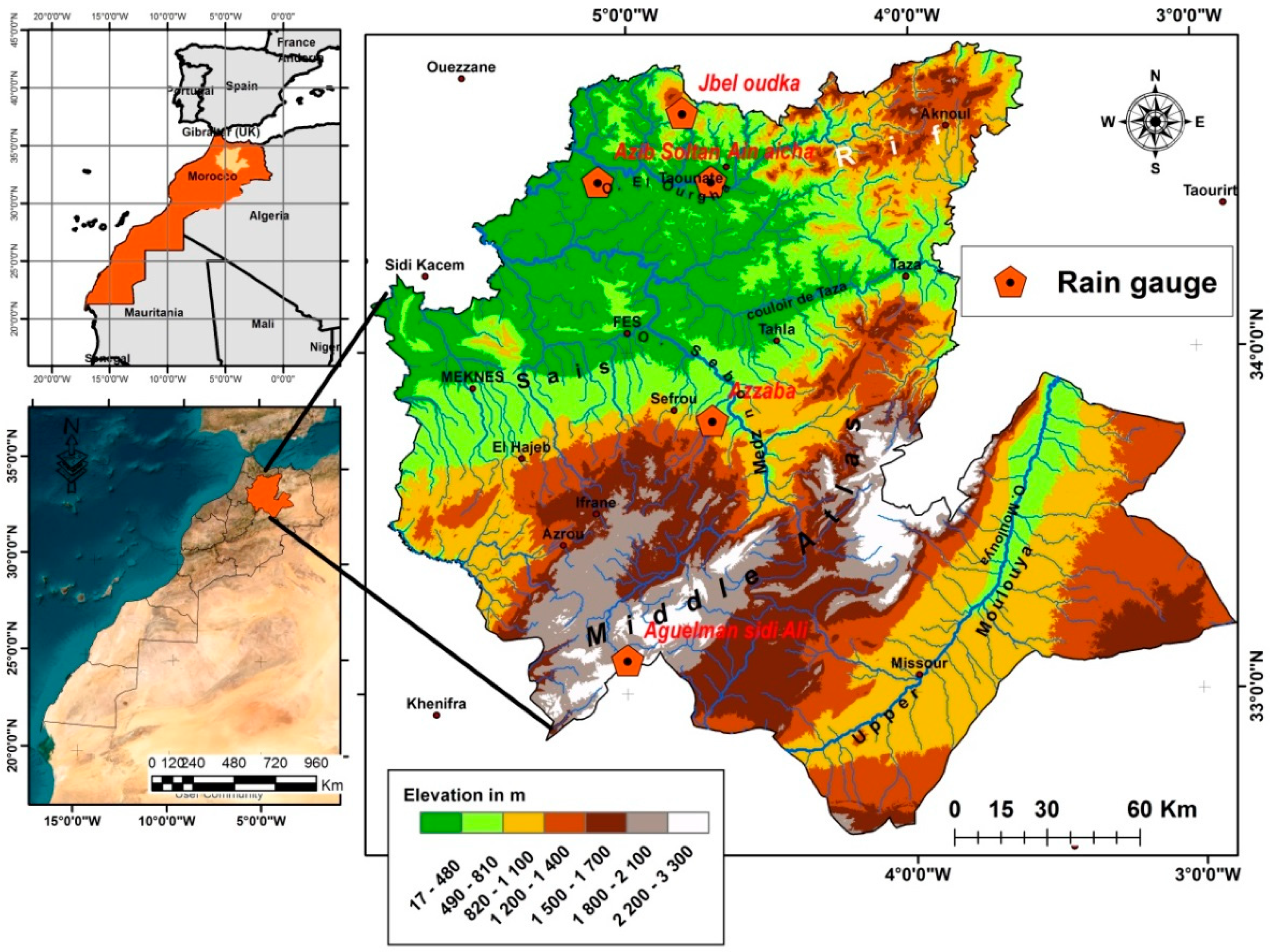
2.1. Presentation of the Study Area

The Fez-Meknes region is one of Morocco’s twelve regions established under the 2015 territorial division. Covering an area of 40,075 km2 and a population of 4.23 million [27], the Fez-Meknes region ranks fourth in terms of both demographic weight and GDP contribution, accounting for 9.39% of the national GDP. The region holds around 15% of the national useful agricultural area, 15% of the national production of cereals, and 14% of the national forests [28].

2.2. Station Rain Gauge Data

Precipitation data were obtained from five weather stations in the region; three of them are located in the north of the region, while the other two are located in the center and south (Figure 1 and Table 1). Two of them are located in a mountainous area, and the other three stations are located in the lowland or foothills. The data on rainfall used in this work were provided by the Hydraulic Basin Agency of Sebou (ABHS), which is the authority in charge of water resources monitoring and management in the watershed of Sebou, Fez, Morocco. They cover monthly precipitation totals from 36 years of measurements from 1982 to 2017 at the five rain gauge stations.

2.3. TerraClimate Data

The TerraClimate dataset (http://www.climatologylab.org/terraclimate.html, accessed on 8 March 2022), developed by scientists at the University of Idaho, has been presented in detail by Abatzoglou et al. [4]. TC is a high spatial and temporal resolution dataset, about 4 km, with monthly data. These are perfectly in line with our objective to compare the precision of precipitation based on downscaled reanalysis data with those obtained from the rain gauge station network. They are obtained from the coarser resolution temporal anomaly downscaling procedures from Climate Research Unit Time Series Data Version 4.0 (CRU Ts4.0) and Japanese reanalysis over 55 years (JRA-55) from 1958 to 2015 with high-resolution climatological fields from WorldClim [29]. The choice of TerraClimate data is motivated by the fact that these data have shown their performance on a global scale. However, ref. [4] clarifies that lower-than-normal correlations for annual precipitation were often found next to stations with a high correlation, suggesting that precipitation can vary on relatively small spatial scales, especially when convective or orographic features are involved that influence the spatial variability of precipitation anomalies at finer scales than those resolved by CRU Ts4.0. Alternatively, subnormal correlations can also arise from potential inhomogeneities or errors in station-based precipitation records.
TC data was extracted from grid cells where the observing stations are located. Since global products, such as TC, are usually affected by bias, TC will be validated, and biases will be corrected using the quantile mapping method.

3. Bias Validation and Correction Methodology

3.1. Validation of Monthly Rainfall Data from TerraClimate

Validation consists of comparing observed and estimated monthly data. In addition to the graphical method, three categories of statistical criteria, often recommended in the literature [30,31], were chosen to measure the robustness of the TerraClimate monthly precipitation data (Table 2).

3.1.1. Correlation Coefficient

As the square of the correlation coefficient R which measures the degree of collinearity between the observed and estimated data, the coefficient of determination R2 expresses the variance of the observed data explained by the TerraClimate data. R2 ranges from 0 to 1; higher values indicate less error variance, and generally, values greater than 0.5 are considered acceptable [32]. Although this coefficient is widely used to evaluate models, it is very sensitive to high extreme values (some of which may be outliers) and insensitive to additive and proportional differences between the estimated values and the measured data [30].
Table 2. Methods for validating monthly TerraClimate rainfall data (E: Monthly rainfall data estimated by TC; O: Monthly rainfall data observed; N: Number of years of observed monthly rainfall data).
CriteriaDefinitionUnit
ME = 1 N i = 1 N E i O i Mean error between estimated (E) and observed (O).(mm)
M A E = 1 N i = 1 N E i O i Mean absolute error between estimated (E) and observed (O).(mm)
MSE = 1 N i = 1 N E i O i 2 Mean squared error between estimated (E) and observed (O).(mm2)
RMSE = 1 N i = 1 N E i O i 2 Root Mean Square Error (RMSE) between estimated (E) and observed (O). RMSE gives the standard deviation of the model prediction error. A smaller value indicates better model performance.(mm)
PBIAS = 100 i = 1 N E i O i i = 1 N O i Percent bias (PBIAS) measures the average tendency of the estimated values to be larger or smaller than their observed ones. The optimal value of PBIAS is 0.0, with low-magnitude values indicating accurate TerraClimate data. Positive values indicate overestimation bias, whereas negative values indicate underestimation bias.(%)
R 2 Coefficient of Determination.(-)
d = 1 i = 1 N O i E i 2 i = 1 N E i O ´ + O i O ´ 2 The Index of Agreement (d) developed by [33] as a standardized measure of the degree of TerraClimate prediction error and varies between 0 and 1. A value of 1 indicates a perfect match, and 0 indicates no agreement at all [33]. The index of agreement can detect additive and proportional differences in the observed and estimated means and variances; however, it is overly sensitive to extreme values due to the squared differences [30].(-)

3.1.2. Index of Agreement

The index of agreement (d) represents the ratio of mean square error to “potential error” [33]. The potential error is the sum of the squared absolute values of the distances between the predicted values and the mean observed value and of the distances between the observed values and the mean observed value. However, d is too sensitive to extreme values due to the use of squared differences [30]. These authors suggested a modified concordance index that is less sensitive to large extreme values because errors and differences are given appropriate weight by using the absolute value of the difference instead of using the squared differences.

3.1.3. Measures of Error

Several error indices are commonly used in model evaluation. They include Mean Error (ME), Mean Absolute Error (MAE), and Root Mean Square Error (RMSE). These indices are valuable because they indicate an error in the units of the data used (or units squared), which facilitates the analysis of the results. Values close to 0 indicate a perfect fit. Ref. [34] indicate that RMSE and MAE values less than half the standard deviation of the measured data can be considered low and that either is appropriate for model evaluation.
Percentage bias (PBIAS) measures the average tendency of estimated data to be larger or smaller than observed data [35]. The optimal value of PBIAS is 0, with low magnitude values indicating an accurate estimate by TerraClimate data. Positive values indicate model underestimation bias, and negative values indicate model overestimation bias [35].

3.1.4. Graphical Comparison

These statistical methods are accompanied by the graphical method, which consists of superimposing the curves of the observed and estimated values of TC. Graphical techniques provide a visual comparison of estimated and measured data [36] and insight into the performance of TerraClimate data. According to [30], graphical techniques are essential for the proper evaluation of models.

3.2. Quantile Mapping Bias-Correction Methods

The qmap (Statistical Transformations for Post-Processing Climate Model Output) package, developed in R [37], was used for bias correction of TC rainfall data. Five variant quantile mapping methods were chosen (Table 3) and are compared with each other using the Taylor diagram [38]. The latter provides a means of graphically summarizing how much TC data differs from observed data and the robustness of the five methods of correcting for this bias. The similarity between the observed data and those estimated by TC, on the one hand, and the data corrected for their biases, on the other hand, is quantified according to their correlation, their centered root mean square difference, and the amplitude of their variations (represented by their standard deviations).

4. Results

4.1. Validation of TC Monthly Rainfall before Bias Correction

According to the values of the coefficient of determination R2, the variance of the station observations explained by the TC data is substantial during the September–June period, during which it exceeds 50% for almost all the stations. It decreases for the months of September in Aguelmane Sidi Ali and Jbel Outhka and May in Azib Soltan. During the dry season (JJA) and with the exception of the Aguelmane Sidi Ali station, there is a high explained variance (above 70%) during the month of June for all the stations, while the variance explained is almost insignificant for July and August. Thus, the TC data capture the inter-annual variability of the monthly rains of the rainy season resulting from the disturbances linked to the passage of the polar front of the winter season. On the other hand, the interannual variability of the convective rains of the hot season (which typically are only a small percentage of annual precipitation and water resources) are less taken into account in the TC data. In addition, the accuracy of monthly rainfall estimates by TC, expressed by the “d” index of [33], is high for the same September–June period.
The absolute error index MAE shows mostly positive values in the Aïn Aïcha and Azzaba stations and mostly negative for the other three stations. It decreases for the months of September in Aguelmane Sidi Ali and Jbel Outhka and May in Azib Soltan. Thus, the TC data captures the inter-annual variability of the months of the rainy season resulting from the disturbances linked to the passage of the polar front of the winter season. On the other hand, the interannual variability of the convective rains of the hot season are less taken into account in the TC data. In addition, the accuracy of monthly rainfall estimates by TC, expressed by the “d” index of [33], is high for the same September–June period. Aguelmane Sidi Ali, Azib Soltane, and Jbel Outhka. Positive MAE values mean that the TerraClimate data overestimates the observed monthly precipitation and vice versa. This over-estimation (or under-estimation) by the TC data remains, on the whole, acceptable for all the stations. Indeed, the TC estimation errors are specified using the values of the MAE and RMSE indices which are compared to half the standard deviation of the observed data, as recommended by [42]. The latter considers that the estimation errors are low when the RMSE and MAE values are less than half the standard deviation of the measured data. According to the criterion based on the MAE values, the error in estimating monthly precipitation by TC is acceptable for the majority of the months and for all the stations, whereas January is the only month of the year during which the estimate is accepted for all stations. However, the examination of the RMSE values, according to the same criterion of [42], attests to the inaccuracy of rainfall estimates for the majority of months at all stations.
PBIAS (in %) measures the average tendency of estimated data to be larger or smaller than their observed data [35]. The sign, positive or negative, shows, respectively, the bias of overestimation or underestimation by the TC data. At high altitude stations (i.e., Aguelmane Sidi Ali, and Jbel Outhka), rainfall is underestimated for all months of the year. This result confirms the difficulty of TC data to take into account the orographic effect in the genesis of rainfall. On the other hand, the estimates of the monthly precipitations at the level of the stations Aïn Aïcha and Azib Soltane, which are marked by their latitudinal and topographical similarities, are divergent: monthly rainfall is generally over-estimated in Aïn Aïcha and under-estimated in Azib Soltane. The Azzaba station, located in the foothills of the Middle Atlas, shows a great similarity in these PBIAIS results with the Aïn Aïcha station. The hot season rains from June to July are underestimated. Thus, the convective processes responsible for summer rains, especially in the mountains, are not sufficiently well taken into account in the TC data.

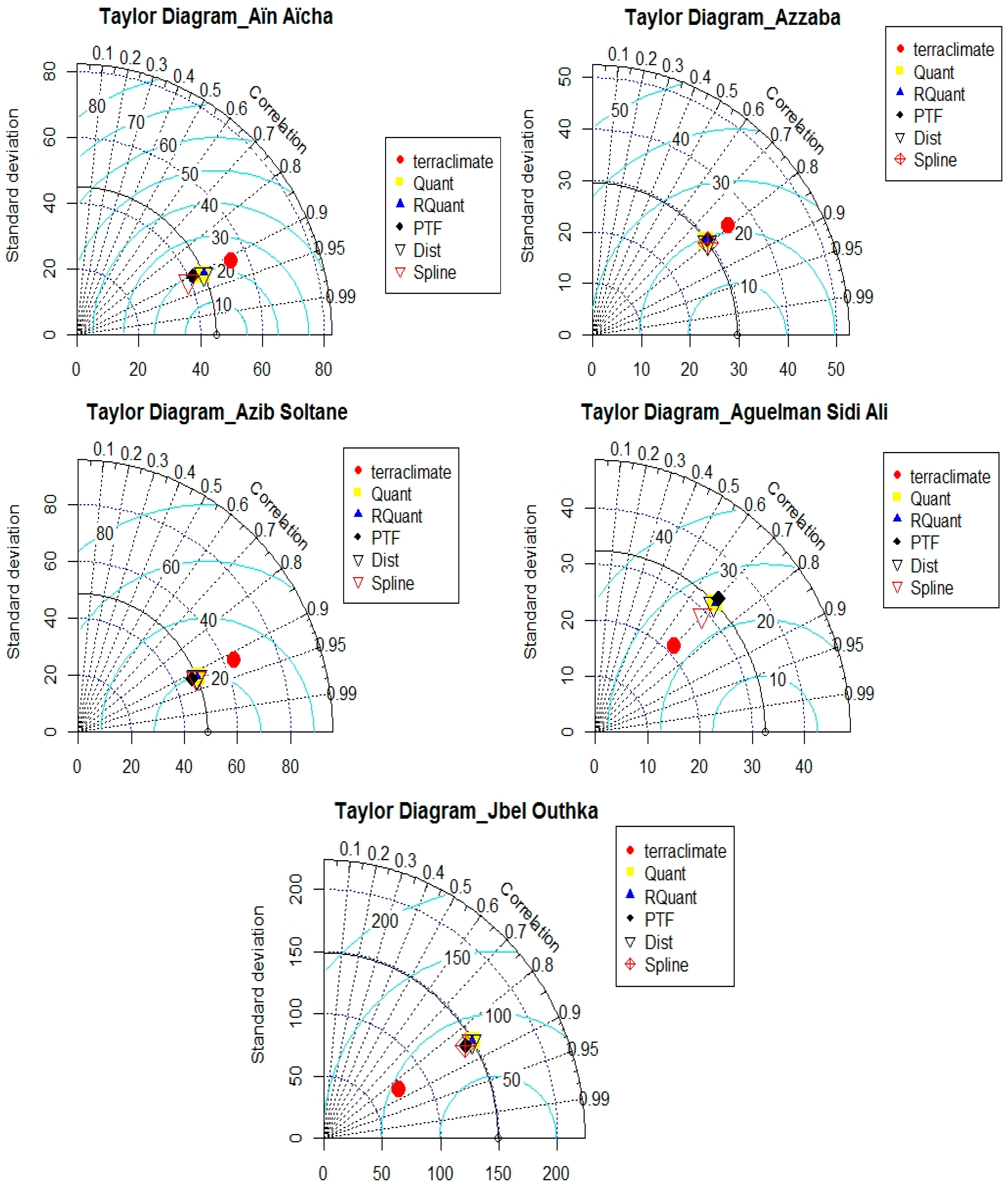
4.2. Validation of Bias Correction Methods for TC Rainfall Data Using the Taylor Diagram

To correct the biases in the precipitation estimated by TC compared to the observed data, the quantile mapping method is used by the station and for the monthly data set. To do this, we used the “qmap” package developed in R [37]. The robustness of the five bias correction methods (Table 2) was evaluated using the Taylor diagram (Figure 2).
The statistics of TC rainfall data observed data and TC corrected by the five methods were calculated, and a symbol was assigned to each type of data. The position of each letter, appearing on the Taylor chart, quantifies how well the TC data and the corrected data match the observed rainfall data. The centered root mean square (RMS) difference between the estimated/corrected and observed data is proportional to the distance to the point on the horizontal axis identified as “observed”. The standard deviation of the estimated/corrected data is proportional to the radial distance from the origin. The standard deviation of the observed data is indicated by the solid line arc. The robustness of the different methods can be deduced from the different figures above. Methods that agree well with observations lie near the “observed” point on the x-axis. This position on the Taylor chart means that the estimated data has a relatively high correlation and low RMS errors. Methods located on the solid line arc have a standard deviation that is equal to the observed data; this means that the observed and estimated data have the same amplitude of variation.
The results obtained do not show a clear improvement in the values of the correlation coefficients between the rainfall data observed and estimated after the correction of the bias by the five methods. All the same, these correlation coefficients remain high and statistically significant at the threshold α = 0.05 for all the TC data and the data corrected by the five bias correction methods.
Furthermore, the five methods showed improvement in the agreement between observed and estimated data, particularly in terms of variability expressed by the standard deviation (SD) values. The five methods clearly improve the values of the SD, which become equal to those of the observed data. This is observed especially for the stations of Azib Soltane and Azzaba. This perfect agreement of the SD values between the observed and estimated data is observed for the four methods (Quant, RQuant, Spline, and PTF) at the Aguelmane Sidi Ali station and for three methods at the Aïn Aïcha station (Quant, RQuant and PTF) and Jbel Outhka (Quant, RQuant, and Spline). We note that the SD values of the TerraClimate data are significantly lower than those of the data observed for the stations of Jbel Outhka and Aguelmane Sidi Ali. The opposite is observed for the other three stations. This result confirms the robustness of bias correction by the five methods that are observed in the TerraClimate data.
The bias correction methods for the TerraClimate data have made it possible to bring a slight improvement to the RMS error values by minimizing the error in estimating the rainfall data, except for the Aguelmane Sidi Ali station where the RMS has slightly increased (RMSterraclimate = 23 mm versus RMSunbiased = 25 mm). This estimation error is of the same order of magnitude for all the methods at the stations of Aïn Aïcha, Azzaba, and Azib Soltane (RMS = 20 mm) and Aguelmane Sidi Ali (RMS = 23 mm), with the exception of the of Jbel Outhka station where it is significantly high (RMS = 80 mm).

4.3. Validation of TC Monthly Rainfall Data after Bias Correction

As for the TC-biased data (Table 4), the values of the coefficient of determination R2 also remain significant for the TC-unbiased data. This has also been shown in Taylor diagrams. Similarly, the accuracy of the estimates, expressed by the “d” index of [33], remains quite high for monthly rainfall TC with or without bias. All the same, there is a slight improvement in the values of R2 and the “d” index during the October-April rainy season, especially at the Jbel Outhka station. Therefore, it seems that the bias correction methods significantly improve the correlations and the accuracy of the estimation of monthly rainfall in mountainous regions. However, we note a clear deterioration in the values of the R2 coefficient and the “d” index in May for all the stations after the correction of the TC data bias.
After the correction of the TC data bias, there is a marked improvement in the estimates of the monthly rainfall data. Indeed, according to the different values of ME, MAE, MSE, and PBIAIS, the estimated reduction in monthly rainfall, with a few exceptions, is significantly improved, especially during the October–pril rainy season. According to the criterion of [34], the MAE values indicate that the error of estimation of monthly precipitation by TC-unbiased is significantly improved for the majority of months and for almost all stations. However, the examination of the RMSE values, according to the same criterion of [34], once again attests to the inaccuracy of the rainfall estimate for the majority of the months at all the stations.

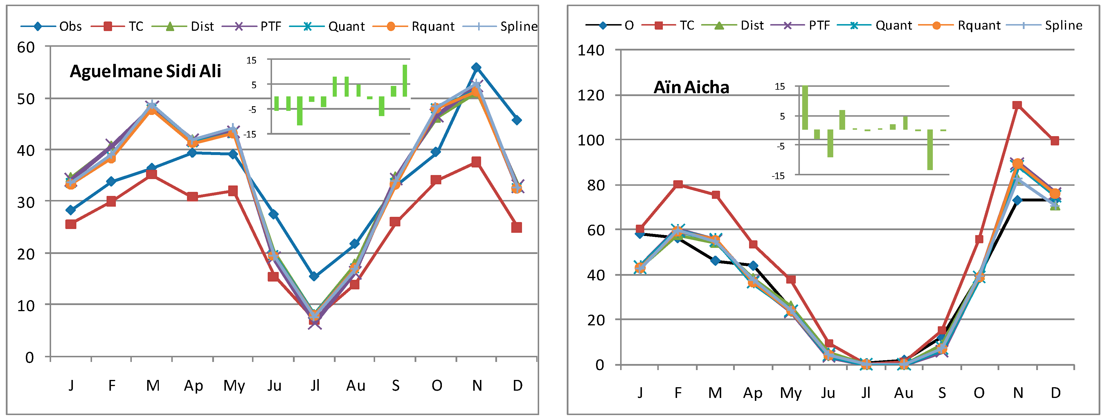
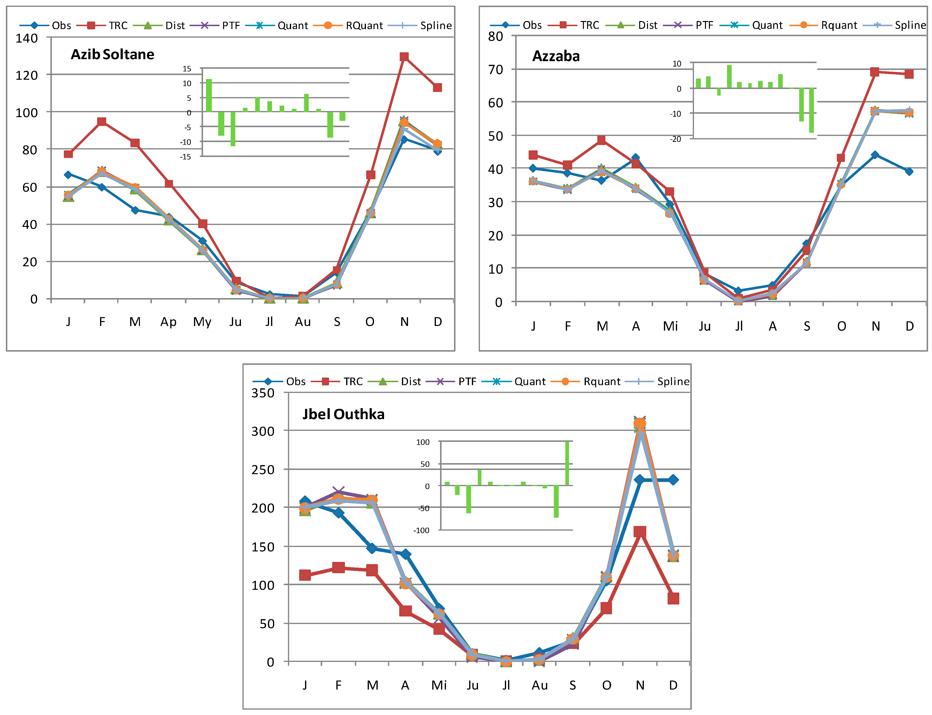
4.4. Comparisons of Average Monthly Rainfall Patterns Observed and Estimated by TerraClimate

4.4.1. Comparisons of Rainfall Patterns before Bias Correction

The monthly rainfall pattern is a crucial indicator for describing the yearly distribution of rainfall, as it affects forest and agricultural ecosystems.
The results of the figures below show a large overestimation of monthly rainfall data by TerraClimate data for two stations (Aïn Aicha and Azib Soltane) and a moderate overestimation at the Azzaba station. However, there is a high underestimation at Aguelman Sidi Ali and Jbel Outhka stations. Therefore, we find two main types of error of under- and over-estimation in mountainous and plain regions, respectively. These errors mark the season going from September to May, while the rhythm of the rain regimes is well respected for all the stations, with a maximum in November and a minimum in July. This is one of the main characteristics of the average Mediterranean rainfall regime in Morocco, which is captured by the TC data.
According to the ME values, the overestimates and underestimates observed before the bias correction were improved in the stations of Aïn Aïcha-Azzaba and Azib Soltane-Aguelmane Sidi Ali-Jbel Outhka, respectively.

4.4.2. Comparisons of Rainfall Patterns after Bias Correction

After the correction of the bias by the five quantile methods, we note their significant correction efficiency, which, however, varies across the stations, with no one method being clearly better than the others. Thus, we calculated the average of the monthly precipitations estimated by the five methods that we compared with the observed values. The results are presented in the form of histograms inside the figures (Figure 3). Negative deviations indicate underestimation by bias correction methods, while positive deviations show the opposite. For the first four stations, the maximum deviations are +/−15 mm, while they are between -70 and +100 mm for the Jbel Outhka station. This large difference is explained by the smaller scale pluviometric contributions that this mountain station receives compared to the others.
By observing the differences between TC and observations per station and per month, we deduce the following remarks:
  • All stations show an overestimation of March rainfall;
  • Unlike the Aguelman Sidi Ali station, the other stations show an underestimation of January and April rainfall and an overestimation of January rainfall;
  • The Azzaba station is unique in its underestimation of April rainfall, unlike the other stations;
  • September rainfall is underestimated at Azib Soltane, Azzaba, and Aïn Aicha stations;
  • Except for Aïn Aicha and Azib Soltane stations, October rainfall is overestimated at the other three stations;
  • Rainfall in December is significantly underestimated at mountain stations (Aguelman Sidi Ali and Jbel Outka) compared to the three low-altitude stations;
  • Summer rainfall is substantially underestimated at the Aguelman Sidi Ali station;
  • May rainfall estimation is relatively accurate across all stations when compared to the other months.

4.4.3. Effectiveness of Bias Correction by Quantile Methods

The degree of effectiveness of the bias correction methods is assessed by comparing both the deviations between the observed data and the data estimated by TerraClimate and the observed data and the corrected TerraClimate data. Given that the results of the correction of the bias by the five methods are almost identical and that the nuances are difficult to distinguish between them, we calculated their average value, which we compared with the monthly values (Figure 4).
According to the results obtained, we notice a clear reduction in the error of estimation of the rains of October–December and March after correction of the bias for the low altitude stations (Aïn Aicha, Azib Soltane, and Azzaba). This marked improvement in rainfall is noted for the month of December in all the stations and the month of November for the four stations, except Jbel Outhka. For this last high mountain station of the Rif, a marked improvement in the estimate of precipitation after correction of the bias is observed for all the months of the year except for the months of March and November. As for the second high mountain station, located in the Middle Atlas, there is a marked improvement in the estimation of rainfall in the hot season (April to September). This station is distinguished by relatively large rainfall events during the hot season. On the other hand, during the period January–March and October, rainfall is overestimated after bias correction; this is observed much more in the month of March.

5. Discussion

Generally, the TC data are able to capture the altitudinal precipitation gradient and the average rainfall regime, with a maximum in November and a minimum in July which is a characteristic of the Mediterranean climate. However, summer precipitation is quite overestimated in mountain regions (case of the Aguelmane Sidi Ali station). These findings agree with those of [15]. TC data have been shown to be in good agreement with ERA/MRCM data, especially over northwestern Morocco, although the latter does not fully capture the bimodal distribution with two peaks in December and March, as evidenced by TC [15]. Furthermore, the validation statistic for TerraClimate was observed to be better than its parent Climate Research Unit (CRU Ts4.0) dataset due to improved spatial realism [14].
Precipitation statistics estimated by models are generally affected by a positive bias in the number of rainy days [16]. Dubey et al., 2021 [14] point out that the estimates of monthly average precipitation by many models, including TC, are also biased. Ref. [15] specify that this bias comes from the imperfect representation of physical processes by the models. Nevertheless, as mentioned above, all model data represent climatological characteristics quite well [14].
However, as reported by [15,16], we found systematic biases, negative in mountainous regions and positive in lowland stations. Ref. [43] Associated model data error with complex topography or atmosphere-biosphere transition with large water bodies. In another study, Allen and Stott (2003) [44] consider climate model errors as an indication of the existence of underrepresented amplification or dampening mechanisms in the model.
Indeed, TC underestimated the orographic effect, which, in reality, performs a role in the intensification of the rains. This underestimation in mountainous regions is systematically observed in all general circulation model (GCM) simulations in the Moroccan Middle Atlas by Tuel et al., 2021 [15], which can be partly explained by the limitations of model grids in resolving orographic precipitation gradients. TC overestimates rainfall in the plains. This was also observed for the TC precipitation of the DJF months on the Moroccan coasts [15]. Moreover, according to the values of the standard deviation, the variability of the monthly rainfall of the TC data, in comparison with the observed data, is high in the plains, while it is very low in the mountainous regions. This bias in the values of the standard deviation has also been observed by [16].
To reduce this bias, different methods can be used [45]. In this study, we applied the method of quantile mapping (QM), which consists of correcting the CDF (Cumulative Distribution Function) of the model output so that it corresponds to the observed one. The usefulness of the method has been highlighted by many authors [23,24,25,45]. Although this technique has its limits, the conclusions drawn from numerous studies, cited by [45], suggest that the QM method outperformed the different methods. Indeed, it leads to the good performance of precipitation data obtained by models [25]. Biases in the simulation of climate models are usually detected by validation (i.e., comparison with observation) according to statistical methods [45]. Validation results were performed using various criteria recommended by several authors [30,31,46].
Although the QM method shows variable performance on spatial and temporal scales, it does not consistently improve after corrections on seasonal and annual time scales [45]. For the case of Morocco, ref. [15] showed that bias-corrected precipitation is slightly lower than observations over the High Atlas and Anti-Atlas. According to our results in the Rif and the Middle Atlas (Jbel Outhka and Aguelman Sidi Ali), this finding cannot be generalized to all months. Prior to bias correction, the TC data is arguably less robust in this region. Indeed, a clear improvement is noted after correction according to the QM method for all the stations and for the majority of the months, with the exception of May. The validation statistics associated with the five QM bias correction methods do not show the robustness of any particular method. Indeed, the results show that most of the QM methods present a reasonable improvement of the TC data after bias corrections on the monthly scale. As pointed out by [23], the QM method, as applied here corrects the full distribution, independent of months, but does not correct all errors in the annual cycle. This correction mainly concerns the improvement of the interannual variability, which is expressed by the standard deviation. Moreover, the robustness of the QM method is observed for the majority of the months of the rainy season. Bias correction significantly improves the average monthly rainfall regime, accurately capturing the wet and dry seasons typical of the Mediterranean climate.

6. Conclusions

The existence of uncertainties, even after corrections of the bias of the TC data, leads us to propose the use of other reanalysis data in order to be able to compare the performance of the model data in our region. This has not been the subject of in-depth studies on this question, with the exception of that of Tuel et al. (2021) [15]. The latter specifies that in the regions of the Middle Atlas, the GCM data underestimate the rainfall in mountainous regions and concludes that the problem of topography is not always resolved. However, our results show that the correction of the TC data bias by the QM method significantly improved the rainfall on the mountain peak of Jbel Outhka. This result must be verified for other high mountain locations. However, given the very weak network of meteorological observations in mountainous regions in Morocco, the TC data with bias correction based on the available stations have good potential. Bias correction is also necessary for stations located on plains and foothills. If improvement remains unsatisfactory after using bias correction approaches, this suggests the existence of complex dynamic processes that cannot be resolved in the global data set.
The rainfall observation network in Morocco is weak, resulting in data containing gaps and being difficult to access. Data from reanalyses can resolve its constraints and gaps. The use of this data in Morocco is very limited. Thus, the assessment of precipitation from TC (this study) or other products is an important research perspective for researchers and policymakers. It allows them to select the most accurate reanalysis data for various applications and to inform users about the various uncertainties in the bases and specifications of these data. The results presented here suggest that the outputs of these models should be cautiously generalized by water resource planners and managers.

Author Contributions

Conceptualization, M.H. and R.K.; methodology, M.H.; software, M.H.; validation, N.Y.K., M.H. and R.K.; formal analysis, M.H.; investigation, R.K. and J.E.K.; resources, A.S.; data curation, M.H.; writing—original draft preparation, R.K.; writing—review and editing, N.Y.K.; visualization, M.H. and I.A.; supervision, M.H. All authors have read and agreed to the published version of the manuscript.

Funding

This research received no external funding.

Data Availability Statement

The data presented in this study are available on request from the corresponding authors.

Acknowledgments

We thank the ABHS staff for providing data.

Conflicts of Interest

The authors declare no conflict of interest.

References

  1. Rodriguez-Iturbe, I.; De Power, B.F.; Sharifi, M.B.; Georgakakos, K.P. Chaos in rainfall. Water Resour. Res. 1989, 25, 1667–1675. [Google Scholar] [CrossRef]
  2. Hamed, M.M.; Nashwan, M.S.; Shahid, S. Performance evaluation of reanalysis precipitation products in Egypt using fuzzy entropy time series similarity analysis. Int. J. Climatol. 2021, 41, 5431–5446. [Google Scholar] [CrossRef]
  3. Tramblay, Y.; Koutroulis, A.; Samaniego, L.; Vicente-Serrano, S.M.; Volaire, F.; Boone, A.; Le Page, M.; Llasat, M.C.; Albergel, C.; Burak, S.; et al. Challenges for drought assessment in the Mediterranean region under future climate scenarios. Earth-Sci. Rev. 2020, 210, 103348. [Google Scholar] [CrossRef]
  4. Abatzoglou, J.T.; Dobrowski, S.Z.; Parks, S.A.; Hegewisch, K.C. TerraClimate, a high-resolution global dataset of monthly climate and climatic water balance from 1958-2015. Sci. Data 2018, 5, 170191. [Google Scholar] [CrossRef] [PubMed]
  5. Centella-Artola, A.; Bezanilla-Morlot, A.; Taylor, M.A.; Herrera, D.A.; Martinez-Castro, D.; Gouirand, I.; Sierra-Lorenzo, M.; Vichot-Llano, A.; Stephenson, T.; Fonseca, C.; et al. Evaluation of Sixteen Gridded Precipitation Datasets over the Caribbean Region Using Gauge Observations. Atmosphere 2020, 11, 1334. [Google Scholar] [CrossRef]
  6. Abdi, O. Climate-Triggered Insect Defoliators and Forest Fires Using Multitemporal Landsat and TerraClimate Data in NE Iran: An Application of GEOBIA TreeNet and Panel Data Analysis. Sensors 2019, 19, 3965. [Google Scholar] [CrossRef]
  7. Wu, B.; Ma, Z.; Yan, N. Agricultural drought mitigating indices derived from the changes in drought characteristics. Remote Sens. Environ. 2020, 244, 111813. [Google Scholar] [CrossRef]
  8. Spinoni, J.; Barbosa, P.; De Jager, A.; McCormick, N.; Naumann, G.; Vogt, J.V.; Magni, D.; Masante, D.; Mazzeschi, M. A new global database of meteorological drought events from 1951 to 2016. J. Hydrol. Reg. Stud. 2019, 22, 100593. [Google Scholar] [CrossRef] [PubMed]
  9. Wang, R.; Zhang, J.; Wang, C.; Guo, E. Characteristic Analysis of Droughts and Waterlogging Events for Maize Based on a New Comprehensive Index through Coupling of Multisource Data in Midwestern Jilin Province, China. Remote Sens. 2019, 12, 60. [Google Scholar] [CrossRef]
  10. Elnashar, A.; Wang, L.; Wu, B.; Zhu, W.; Zeng, H. Synthesis of global actual evapotranspiration from 1982 to 2019. Earth Syst. Sci. Data 2021, 13, 447–480. [Google Scholar] [CrossRef]
  11. Hu, Y.; Han, Y.; Zhang, Y. Land desertification and its influencing factors in Kazakhstan. J. Arid Environ. 2020, 180, 104203. [Google Scholar] [CrossRef]
  12. Khan, R.; Gilani, H.; Iqbal, N.; Shahid, I. Satellite-based (2000–2015) drought hazard assessment with indices, mapping, and monitoring of Potohar plateau, Punjab, Pakistan. Environ. Earth Sci. 2019, 79, 23. [Google Scholar] [CrossRef]
  13. Salhi, A.; Martin-Vide, J.; Benhamrouche, A.; Benabdelouahab, S.; Himi, M.; Benabdelouahab, T.; Casas Ponsati, A. Rainfall distribution and trends of the daily precipitation concentration index in northern Morocco: A need for an adaptive environmental policy. SN Appl. Sci. 2019, 1, 277. [Google Scholar] [CrossRef]
  14. Dubey, S.; Gupta, H.; Goyal, M.K.; Joshi, N. Evaluation of precipitation datasets available on Google earth engine over India. Int. J. Climatol. 2021, 41, 4844–4863. [Google Scholar] [CrossRef]
  15. Tuel, A.; Kang, S.; Eltahir, E.A.B. Understanding climate change over the southwestern Mediterranean using high-resolution simulations. Clim. Dyn. 2021, 56, 985–1001. [Google Scholar] [CrossRef]
  16. Piani, C.; Haerter, J.O.; Coppola, E. Statistical bias correction for daily precipitation in regional climate models over Europe. Theor. Appl. Climatol. 2010, 99, 187–192. [Google Scholar] [CrossRef]
  17. Ines, A.V.M.; Hansen, J.W. Bias correction of daily GCM rainfall for crop simulation studies. Agric. For. Meteorol. 2006, 138, 44–53. [Google Scholar] [CrossRef]
  18. Sapountzis, M.; Kastridis, A.; Kazamias, A.P.; Karagiannidis, A.; Nikopoulos, P.; Lagouvardos, K. Utilization and uncertainties of satellite precipitation data in flash flood hydrological analysis in ungauged watersheds. Glob. Nest J. 2021, 23, 388–399. [Google Scholar] [CrossRef]
  19. Maghsood, F.F.; Hashemi, H.; Hosseini, S.H.; Berndtsson, R. Ground Validation of GPM IMERG Precipitation Products over Iran. Remote Sens. 2020, 12, 48. [Google Scholar] [CrossRef]
  20. Piani, C.; Weedon, G.P.; Best, M.; Gomes, S.M.; Viterbo, P.; Hagemann, S.; Haerter, J.O. Statistical bias correction of global simulated daily precipitation and temperature for the application of hydrological models. J. Hydrol. 2010, 395, 199–215. [Google Scholar] [CrossRef]
  21. Maraun, D. Bias Correction, Quantile Mapping, and Downscaling: Revisiting the Inflation Issue. J. Clim. 2013, 26, 2137–2143. [Google Scholar] [CrossRef]
  22. Cannon, A.J.; Sobie, S.R.; Murdock, T.Q. Bias Correction of GCM Precipitation by Quantile Mapping: How Well Do Methods Preserve Changes in Quantiles and Extremes? J. Clim. 2015, 28, 6938–6959. [Google Scholar] [CrossRef]
  23. Reiter, P.; Gutjahr, O.; Schefczyk, L.; Heinemann, G.; Casper, M. Does applying quantile mapping to subsamples improve the bias correction of daily precipitation? Int. J. Climatol. 2018, 38, 1623–1633. [Google Scholar] [CrossRef]
  24. Vigna, I.; Bigi, V.; Pezzoli, A.; Besana, A. Comparison and Bias-Correction of Satellite-Derived Precipitation Datasets at Local Level in Northern Kenya. Sustainability 2020, 12, 2896. [Google Scholar] [CrossRef]
  25. Heo, J.-H.; Ahn, H.; Shin, J.-Y.; Kjeldsen, T.R.; Jeong, C. Probability Distributions for a Quantile Mapping Technique for a Bias Correction of Precipitation Data: A Case Study to Precipitation Data Under Climate Change. Water 2019, 11, 1475. [Google Scholar] [CrossRef]
  26. Kessabi, R.; Hanchane, M.; Guijarro, J.A.; Krakauer, N.Y.; Addou, R.; Sadiki, A.; Belmahi, M. Homogenization and Trends Analysis of Monthly Precipitation Series in the Fez-Meknes Region, Morocco. Climate 2022, 10, 64. [Google Scholar] [CrossRef]
  27. HCP. Recensement Général de la Populatiion et de l’Habitat; Monographie Générale; Région de Fès-Meknès. 2014; p. 171. Rabat, Morocco. Available online: https://www.hcp.ma/ (accessed on 23 May 2023).
  28. DGCL. Monographie Générale; Région de Fès-Meknè. 2015; p. 62. Rabat, Morocco. Available online: https://collectivites-territoriales.gov.ma/fr/node/738 (accessed on 23 May 2023).
  29. Ebita, A.; Kobayashi, S.; Ota, Y.; Moriya, M.; Kumabe, R.; Onogi, K.; Harada, Y.; Yasui, S.; Miyaoka, K.; Takahashi, K.; et al. The Japanese 55-year Reanalysis “JRA-55”: An interim report. SOLA 2011, 7, 149–152. [Google Scholar] [CrossRef]
  30. Legates, D.R.; McCabe, G.J., Jr. Evaluating the use of “goodness-of-fit” Measures in hydrologic and hydroclimatic model validation. Water Resour. Res. 1999, 35, 233–241. [Google Scholar] [CrossRef]
  31. Moriasi, D.N.; Arnold, J.G.; van Liew, M.W.; Bingner, R.L.; Harmel, R.D.; Veith, T.L. Model Evaluation Guidelines for Systematic Quantification of Accuracy in Watershed Simulations. Trans. ASABE 2007, 50, 885–900. [Google Scholar] [CrossRef]
  32. Santhi, C.; Arnold, J.G.; Williams, J.R.; Dugas, W.A.; Srinivasan, R.; Hauck, L.M. Validation of the swat model on a large rwer basin with point and nonpoint sources. JAWRA J. Am. Water Resour. Assoc. 2001, 37, 1169–1188. [Google Scholar] [CrossRef]
  33. Willmott, C.J. On the Evaluation of Model Performance in Physical Geography BT—Spatial Statistics and Models; Gaile, G.L., Willmott, C.J., Eds.; Springer: Dordrecht, The Netherlands, 1984; pp. 443–460. ISBN 978-94-017-3048-8. [Google Scholar]
  34. Singh, U.; Agarwal, P.; Sharma, P.K. Meteorological drought analysis with different indices for the Betwa River basin, India. Theor. Appl. Climatol. 2022, 148, 1741–1754. [Google Scholar] [CrossRef]
  35. Gupta, H.V.; Sorooshian, S.; Yapo, P.O. Status of automatic calibration for hydrologic models: Comparison with multilevel expert calibration. J. Hydrol. Eng. ASCE 1999, 4, 135–143. [Google Scholar] [CrossRef]
  36. ASCE Criteria for Evaluation of Watershed Models. J. Irrig. Drain. Eng. 1993, 119, 429–442. [CrossRef]
  37. Gudmundsson, L.; Bremnes, J.B.; Haugen, J.E.; Engen-Skaugen, T. Technical Note: Downscaling RCM precipitation to the station scale using statistical transformations—A comparison of methods. Hydrol. Earth Syst. Sci. 2012, 16, 3383–3390. [Google Scholar] [CrossRef]
  38. Taylor, K.E. Summarizing multiple aspects of model performance in a single diagram. J. Geophys. Res. Atmos. 2001, 106, 7183–7192. [Google Scholar] [CrossRef]
  39. Manatsa, D.; Chingombe, W.; Matarira, C.H. The impact of the positive Indian Ocean dipole on Zimbabwe droughts. Int. J. Climatol. 2008, 28, 2011–2029. [Google Scholar] [CrossRef]
  40. Li, H.; Sheffield, J.; Wood, E.F. Bias correction of monthly precipitation and temperature fields from Intergovernmental Panel on Climate Change AR4 models using equidistant quantile matching. J. Geophys. Res. Atmos. 2010, 115, 520. [Google Scholar] [CrossRef]
  41. Dosio, A.; Paruolo, P. Bias correction of the ENSEMBLES high-resolution climate change projections for use by impact models: Evaluation on the present climate. J. Geophys. Res. Atmos. 2011, 116, 161. [Google Scholar] [CrossRef]
  42. Singh, J.; Knapp, H.V.; Arnold, J.G.; Demissie, M. Hydrological modeling of the Iroquois River watershed using HSPF and SWAT. J. Am. Water Resour. Assoc. 2005, 41, 343–360. [Google Scholar] [CrossRef]
  43. Cardell, M.F.; Amengual, A.; Romero, R.; Ramis, C. Future extremes of temperature and precipitation in Europe derived from a combination of dynamical and statistical approaches. Int. J. Climatol. 2020, 40, 4800–4827. [Google Scholar] [CrossRef]
  44. Allen, M.R.; Stott, P.A. Estimating signal amplitudes in optimal fingerprinting, part I: Theory. Clim. Dyn. 2003, 21, 477–491. [Google Scholar] [CrossRef]
  45. Ayugi, B.; Tan, G.; Ruoyun, N.; Babaousmail, H.; Ojara, M.; Wido, H.; Mumo, L.; Ngoma, N.H.; Nooni, I.K.; Ongoma, V. Quantile Mapping Bias Correction on Rossby Centre Regional Climate Models for Precipitation Analysis over Kenya, East Africa. Water 2020, 12, 801. [Google Scholar] [CrossRef]
  46. Darand, M.; Khandu, K. Statistical evaluation of gridded precipitation datasets using rain gauge observations over Iran. J. Arid Environ. 2020, 178, 104172. [Google Scholar] [CrossRef]
Figure 1. Geographical location of the Fez-Meknes region.
Climate 11 00120 g001
Figure 2. Taylor diagram displaying a statistical comparison of monthly rainfall data observed each year with TC data before and after bias corrections according to five methods.
Climate 11 00120 g002
Figure 3. Comparison of average rainfall patterns observed with TCs before and after bias correction according to five methods (the green bar chart inset inside each graph shows the average deviation between the corrected TCs and the observed data).
Climate 11 00120 g003aClimate 11 00120 g003b
Figure 4. Differences between monthly rainfall data observed and TC before (brown bars) and after bias correction (blue bars).
Climate 11 00120 g004
Table 1. Characteristics of the five rain gauge stations.
Rain Gauge StationLatitude °Longitude °Elevation in (Meters)Mean Annual Precipitation in (mm)T Average in (°C)The de Martonne Aridity IndexClimate
Rain Gauge DataTerra
Climate
Aguelman Sidi Ali33.1−5.02089423.9329.210.021Sub humid
Ain Aicha34.5−4.7236500.4602.818.917Semi-arid
Azib Soltane34.5−5.1298488.9692.419.117Semi-arid
Azzaba33.8−4.7373339.9416.817.712Semi-arid
Jbel Outhka34.7−4.815891515.2817.014.562Humid
Table 3. Characteristics of bias correction methods (source: ‘qmap’ package under R, [37]).
MethodDescriptionReferences
fitQmapQUANT: Non-parametric quantile mapping using empirical quantiles.Estimates values of the empirical cumulative distribution function of observed and modeled time series for regularly spaced quantiles. doQmapQUANT uses these estimates to perform quantile mapping.[37,39]
fitQmapRQUANT: Non-parametric quantile mapping using robust empirical quantilesEstimates the values of the quantile-quantile relation of observed and modeled time series for regularly spaced quantiles using local linear least square regression. doQmapRQUANT performs quantile mapping by interpolating the empirical quantiles.[39]
fitQmapSSPLIN: Quantile mapping using a smoothing splinefitQmapSSPLIN fits a smoothing spline to the quantile-quantile plot of observed and modeled time.
doQmapSSPLIN uses the spline function to adjust the distribution of the modeled data to match the distribution of the observations.
[37]
fitQmapDIST: Quantile mapping using distribution-derived transformationsfitQmapDIST fits a theoretical distribution to observed and to modeled time series and returns these parameters and a transfer function derived from the distribution. doQmapDIST uses the transfer function to transform the distribution of the modeled data to match the distribution of the observations.[16,17,37,40]
fitQmapPTF: Quantile mapping using parametric transformationsfitQmapPTF fits parametric transformations to the quantile-quantile relation of observed and modeled values. doQmapPTF uses the transformation to adjust the distribution of the modeled data to match the distribution of the observations.[20,37,41]
Table 4. Validation results of TC before and after bias correction (values in bold indicate improved estimates (before or after bias correction); underlined values indicate the acceptability of MAE and RMSE values) (SD: Standard Deviation of observed monthly rainfall).
Aïn Aicha_ before bias correctionAïn Aïcha_ after bias correction
MonthME
(mm)
MAE
(mm)
MSE
(mm2)
RMSE
(mm)
PBias
(%)
R2dME
(mm)
MAE
(mm)
MSE
(mm2)
RMSE
(mm)
PBias
(%)
R2dSD
S3.048.43131.811.525.60.50.81−4.217.6149.712.2−35.40.520.7115.92
O16.5820.64667.225.842.20.70.86−0.1512.131217.7−0.40.710.933.29
N42.3544.89273152.3580.80.8113.622.781728.618.60.780.950.39
D26.1932.641699.241.235.80.830.920.5918.873327.10.80.84169.4
J2.3112.427616.640.891−1518.37611.124.7−25.80.90.9250.49
F23.827.1101233.342.40.80.872.6515.749322.24.70.80.945.48
M29.1730.51136336.963.20.780.858.8316.547221.719.10.770.942.05
A29.1730.511363.136.963.20.80.85−6.7813.725919−15.40.660.930.95
M12.715.5347.618.6510.70.9−21.531.48242449.2−46.70.010.4126.22
J5.515.6896.49.82143.10.70.780.632.9425.75.0716.40.670.97.48
J−0.460.462.041.43−100NA0.3−0.460.4621.43−100NA0.261.37
A−0.722.1523.64.86−38.30.10.3−1.851.8528.65.35−980.070.265.14
Azib Soltan_ before bias correctionAzib Soltan_ after bias correction
MonthME
(mm)
MAE
(mm)
MSE
(mm2)
RMSE
(mm)
PBias
(%)
R2dME
(mm)
MAE
(mm)
MSE
(mm2)
RMSE
(mm)
PBias
(%)
R2dSD
S1.467.89106.310.3110.50.740.9−6.378.66207.414.4−45.80.770.718.95
O−3.7415.62427.620.68−80.670.89−1.2813.88397.919.182.70.710.9235.87
N−16.523.541005.531.71−19.30.780.898.6217.98555.223.5910.10.860.9655.63
D−10.820.01885.729.76−13.70.870.933.0718.5273127.043.90.860.9668.69
J−22.525.11777.742.16−33.90.840.8−11.417.25747.327.34−17.20.890.9363.04
F−18.726.081358.436.86−31.30.70.758.0619.65656.925.6313.50.750.9249.45
M0.9416.1409.520.2420.70.911.7218.46564.523.7624.70.750.9137.58
A−2.3211.81266.816.33−5.30.680.9−1.4310.5122715.07−3.30.730.9228.99
M2.1518.6610.524.7170.470.8−21.631.86209245.74−45.50.030.4934.19
J0.394.53446.74.70.730.9−3.74.4363.87.99−44.40.720.8713.08
J−1.292.33255.06−59.10.060.29−2.172.17305.48−100NA0.335.1
A2.272.74123.471880.30.6−1.131.166.82.6−93.50.390.392.55
Azzaba_ before bias correctionAzzaba_ after bias correction
MonthME
(mm)
MAE
(mm)
MSE
(mm2)
RMSE
(mm)
PBias
(%)
R2dME
(mm)
MAE
(mm)
MSE
(mm2)
RMSE
(mm)
PBias
(%)
R2dSD
S−1.949.12208.714.5−11.20.570.8−5.499.24258.816.1−31.70.570.7221.52
O8.1314.23327.518.123.20.790.920.3313.231417.70.90.770.9135.24
N24.9426.91334.836.556.60.580.7213.318.568426.130.10.580.8126
D29.1629.311785.342.274.70.690.7417.819.8100831.745.60.660.8129.18
J3.9412.02288.3179.80.720.91−3.7810.822014.8−9.40.740.9228.2
F2.5110.81179.413.46.50.730.9−4.7910.4194.613.9−12.40.720.925.18
M12.0316.62496.322.333.10.60.813.1412.825115.88.60.610.8721.84
A−1.7917.4981.831.3−4.10.510.8−9.2317.89113033.6−21.40.50.7144.38
M3.9212.4231.615.213.50.670.9−9.5825.43889.229.8−26.400.4325.98
J0.44.3140.76.44.80.770.9−1.713.9145.36.7−21.10.80.9113.42
J−2.232.9242.16.5−71.50.190.33−2.93347.36.9−94.10.220.356.51
A−1.273.6848.97−26.80.530.6−2.553.658.47.6−53.80.480.548.84
Aguelman Sidi Ali_ before bias correctionAguelman Sidi Ali_ after bias correction
MonthME
(mm)
MAE
(mm)
MSE
(mm2)
RMSE
(mm)
PBias
(%)
R2dME
(mm)
MAE
(mm)
MSE
(mm2)
RMSE
(mm)
PBias
(%)
R2dSD
S−7.9117.02531.823−21.30.430.770.8316.47584.624.182.50.440.829.34
O−5.4315.4438.621−13.50.650.867.6617.43495.622.26190.680.934.17
N−10.319.9910.530.2−180.580.8−4.6929.18178142.2−8.20.230.7144.06
D−21.223.841510.738.9−45.40.680.67−13.320.398931.45−28.50.680.8146.9
J−2.668.64143.112−9.20.810.935.659.86177.313.3119.40.820.9426.39
F−3.8913.2340.518. 5−11.20.570.825.7713.79367.319.1716.60.580.8627.63
M−1.1612.1275.616.6−3.10.590.911.617.0652322.87310.60.8426.19
A−8.615.71546.123.4−21.30.60.812.1215.351622.75.20.570.8733.84
M−7.1213.3350.518.7−17.80.660.96.8333.49181242.5718.300.3330.06
J−12.316.951022.6−43.70.370.7−8.1617.42510.322.59−29.10.360.7524.04
J−8.5112.18434.120.9−54.20.020.4−7.8812.54443.221.05−50.20.010.419.2
A−7.991438619. 7−36.10.070.52−4.7915.14402.820.07−21.60.070.5417.78
Jbel Outhka_ before bias correctionJbel Outhka_ after bias correction
MonthME
(mm)
MAE
(mm)
MSE
(mm2)
RMSE
(mm)
PBias
(%)
R2dME
(mm)
MAE
(mm)
MSE
(mm2)
RMSE
(mm)
PBias
(%)
R2dSD
S−3.2316.1674.826−120.450.71.8316.81621.424.96.80.470.8135.67
O−36.242473404.858.3−34.40.620.765.1240.8275552.54.90.60.8773.67
N−67.975.912,390111.3−28.70.760.8171.1189.6214,800121.730.10.750.88165.93
D−14615550,199224.1−65.30.790.6−90.110723,897154.6−41.50.790.81234.33
J−95.7104.521,474146.5−460.890.76−9.0847.2399663.2−4.40.890.97219.64
F−71.388.1119,047138−36.90.610.6820.26910,732103.610.50.620.87177.85
M−28.961.1940997−19.60.640.7991.3985.0612,048109.841.70.670.86146.54
A−7474.41982394.4−530.540.61−36.658.8499570.7−26.20.520.7894.89
M−27.135.113162.756.2−39.20.760.7−86105.629,407171.5−58.40.010.480.11
J−1.665.5275.18.7−16.20.740.9−1.746.0293.19.65−170.740.9217.96
J−0.691.3962.44−44.60.140.5−1.381.467.852.8−88.60.10.42.77
A−8.1210.61172941.6−69.70.210.16−9.6710.51775.742.1−830.190.178.7
Disclaimer/Publisher’s Note: The statements, opinions and data contained in all publications are solely those of the individual author(s) and contributor(s) and not of MDPI and/or the editor(s). MDPI and/or the editor(s) disclaim responsibility for any injury to people or property resulting from any ideas, methods, instructions or products referred to in the content.

