Article

Evaluating the Efficacy of Different DEMs for Application in Flood Frequency and Risk Mapping of the Indian Coastal River Basin

1
Department of Civil Engineering, Dr. S. & S. S. Ghandhy Government Engineering College, Surat 395008, Gujarat, India
2
Department of Hydrology, Indian Institute of Technology Roorkee, Roorkee 247667, Uttarakhand, India
3
Institute for Sustainable Industries & Liveable Cities, Victoria University, Melbourne, VIC 8001, Australia
4
College of Sport, Health and Engineering, Victoria University, Melbourne, VIC 8001, Australia
5
Department of Civil Engineering and Construction, Faculty of Engineering and Design, Atlantic Technological University, F91 YW50 Sligo, Ireland
*
Author to whom correspondence should be addressed.
Climate 2023, 11(5), 114; https://doi.org/10.3390/cli11050114
Submission received: 10 April 2023 / Revised: 13 May 2023 / Accepted: 18 May 2023 / Published: 22 May 2023

Abstract

:
Floods are among the most occurring natural hazards that cause severe damage to infrastructure and loss of life. In India, southern Gujarat is affected during the monsoon season, facing multiple flood events in the Damanganga basin. As the basin is one of the data-scarce regions, evaluating the globally available dataset for flood risk mitigation studies in the Damanganga basin is crucial. In the present study, we compared four open-source digital elevation models (DEMs) (SRTM, Cartosat-1, ALOS-PALSAR, and TanDEMX) for hydrodynamic (HD) modeling and flood risk mapping. The simulated HD models for multiple flood events using HEC-RAS v6.3 were calibrated by adopting different roughness coefficients based on land-use land cover, observed water levels at gauge sites, and peak flood depths in the flood plain. In contrast to the previous studies on the Purna river basin (the neighboring basin of Damanganga), the present study shows that Cartosat-1 DEM provides reliable results with the observed flood depth. Furthermore, the calibrated HD model was used to determine the flood risk corresponding to 10, 25, 50, and 100-year return period floods calculated using Gumbel’s extreme value (GEV) and log-Pearson type III (LP-III) distribution techniques. Comparing the obtained peak floods corresponding to different return periods with the observed peak floods revealed that the LP-III method gives more reliable estimates of flood peaks for lower return periods, while the GEV method gives comparatively more reliable estimates for higher return period floods. The study shows that evaluating different open-source data and techniques is crucial for developing reliable flood mitigation plans with practical implications.

1. Introduction

Floods are one of the most common natural hazards causing devastating impacts worldwide [1,2]. Furthermore, the impacts of floods are increasing due to the encroachment of rivers, settlement in floodplains, changing land-use land cover, and climate change [3,4]. India is frequently affected by floods of different magnitudes every year and suffers enormous economic losses and loss of human lives [5,6,7,8]. Wide variations in rainfall, both in time and space, with frequent departures from the normal pattern, rivers with insufficient carrying capacity, river bank erosion, degradation of hilly catchments and silting of river beds, landslides, poor natural drainage in flood-prone areas, glacial lake outbursts, cloud bursts, and other factors all contribute to frequently occurring floods in India [9,10,11,12].
To prepare reliable flood mitigation plans, understanding flood regimes and causative factors, such as geomorphology, climate, and anthropogenic activities, is essential [13,14]. The information on water levels and flood inundation extent is crucial for preparing flood risk, hazards, and vulnerability maps [15]. In practice, the water level can be measured by river gauge during the flood event and can be used to simulate the flood inundation extent using hydrodynamic (HD) models [16,17]. However, the reliability of the simulated results depends on the model used, its assumption, and its input parameters [13,18]. For quick simulation of water level and flow along the river channel, the one-dimensional (1D) models are preferred, and for simulating the flood inundation extent in the floodplain, the two-dimensional (2D) models are utilized [19,20,21,22]. With the availability of freely available flood models and hydrologic datasets, flood inundation mapping has been eased for different rivers of the world. Despite this, various studies have demonstrated and quantified the uncertainty in the results caused by input data, model parameters, and boundary conditions [23,24]. Among all factors, the roughness coefficient (for channels and floodplains) and digital elevation data (source and resolution) are recognized as highly sensitive factors by many researchers [25,26,27,28,29,30]. For example, the digital elevation model (DEM) includes the elevation of objects and buildings instead of the bathymetry [31], and for the calibration in both 1D and 2D flood models [32], Manning’s roughness coefficient is subsequently optimized to obtain simulated results as close to observed data [16,22]. Nevertheless, river bathymetry plays an important role in the accuracy of flood modeling. Modeling irregular river bathymetry in hydrological models is tricky and causes uncertainty in results [32]. Therefore, 2D models may produce better results compared to 1D models.
Hydrodynamic models are reliable tools for managing urban stormwater. Planning and designing urban drainage systems scientifically, as well as developing effective urban flood disaster control and management strategies, depend on numerical simulations of urban floods. The high-resolution DEMs generated using Light Detection and Ranging (LiDAR) are proven to be the most accurate for hydraulic models [13,33]. As identified by many researchers, these DEMs are not error-free when using it to generate flood inundation and risk maps, especially in low-lying and urban areas [34,35]. Although DEMs are frequently used in hydrologic studies, individuals rarely take into consideration the inaccuracy in the DEM representation of the terrain through elevation and derived topographic parameters [36]. Furthermore, ignoring these errors would generate the wrong prediction while using such models in flood frequency analysis and risk mapping of future flood events. Therefore, there is still a need to investigate the efficacy of the freely available DEMs for flood modeling and inundation mapping, particularly in developing countries where surveyed topography datasets are unavailable.
In the present study, we investigated the efficacy of four different DEMs (SRTM, ALOS-PALSAR, TanDEM-X, and Cartosat-1) for flood inundation and risk mapping in the Damanganga river basin, which is in the flat Indian coastal terrain of Gujarat state. The Hydrologic Engineering Center’s River Analysis System (HEC-RAS v6.3) [37] was utilized to simulate 1D and 2D flood models. Based on the data availability, we calibrated and validated the flood model for three different flood events by comparing the simulated water levels with the observed water levels for different Manning’s roughness coefficients. Furthermore, flood frequency analysis (FFA) was carried out using Gumbel’s extreme value (GEV) [38] and log-Pearson type III (LP-III) [39,40] to determine the probable magnitude of 10, 25, 50, and 100-year return period flood. The present study aims (1) to evaluate the efficacy of different DEMs for flood modeling in low-lying Indian coastal river basins and (2) to generate reliable flood inundation and risk maps of different return periods. The present study will be helpful for the selection of flood model inputs and the development of flood inundation and risk maps in the region where surveyed topographic datasets are unavailable.

2. Study Area and Data Collection
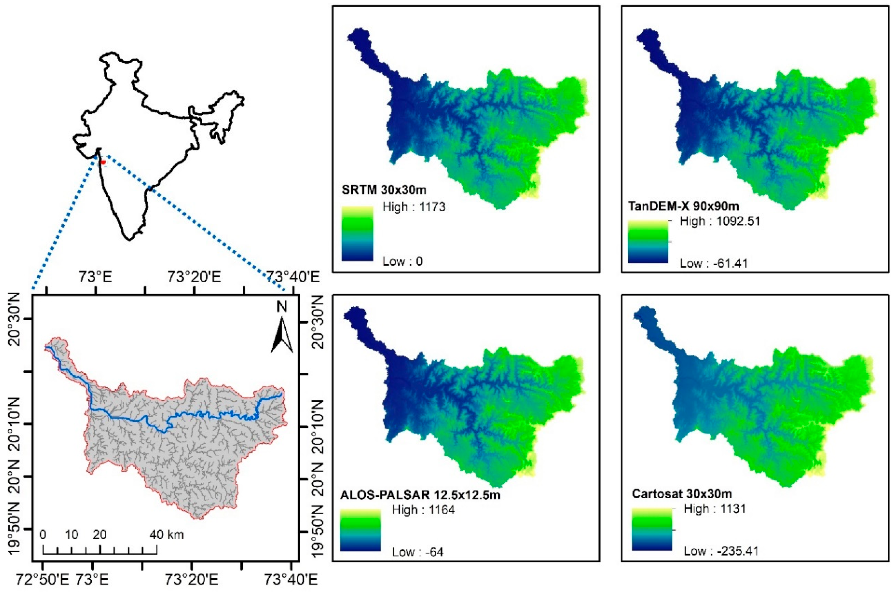
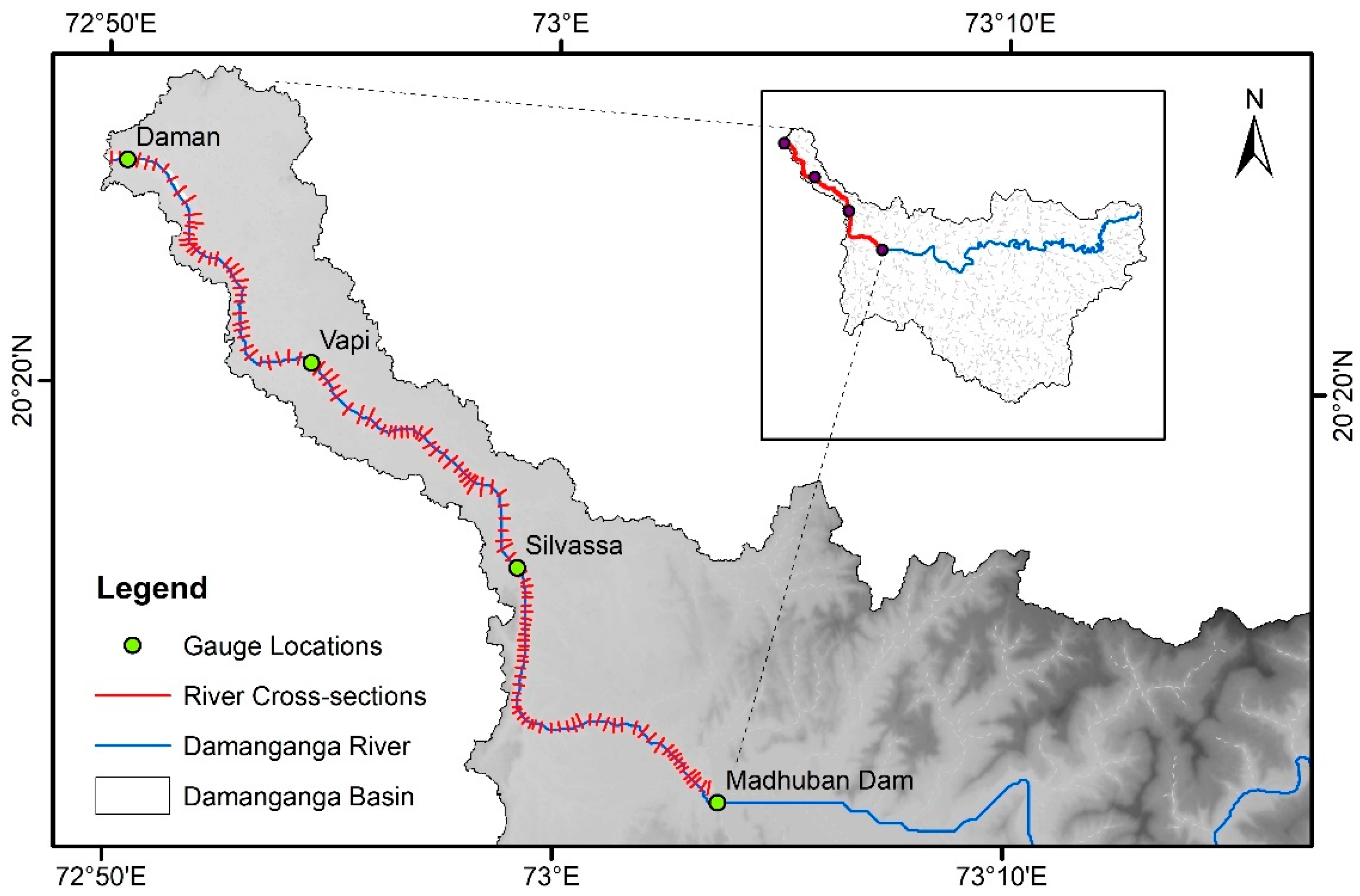
2.1. Study Area

The Damanganga is a western-flowing river that flows north of Mumbai and south of the Tapi River, located between the north latitude of 19°52′–20°26′ and east longitude of 72°50′–73°39′. It has a length of 131.30 km and a basin size of 2318 km2. The river rises near the village Ambegaon in the Dindori taluka of Maharashtra’s Nasik district at an elevation of 950 m above mean sea level and drains into the Arabian Sea near Daman city. The entire Damanganga basin lies in the Western Ghats region between the Arabian Sea in the west and the Sahyadri hills in the east. The southwest monsoon brings the most rain (98% of annual rainfall) to the basin from June to October. The temperature reaches its highest point in May and its lowest point in December and January. The average wind speed in the Damanganga basin ranges from 0.7 to 4.3 km/h, and the relative humidity ranges from 65.5 to 91.9%. Figure 1 shows the location map of the Damanganga river basin, along with the topography obtained from the four DEMs. The highest and lowest elevation of the basin across different DEMs varies from 1092.51 to 1173 m and −235.41 to 0 m, respectively.

2.2. Data Collection
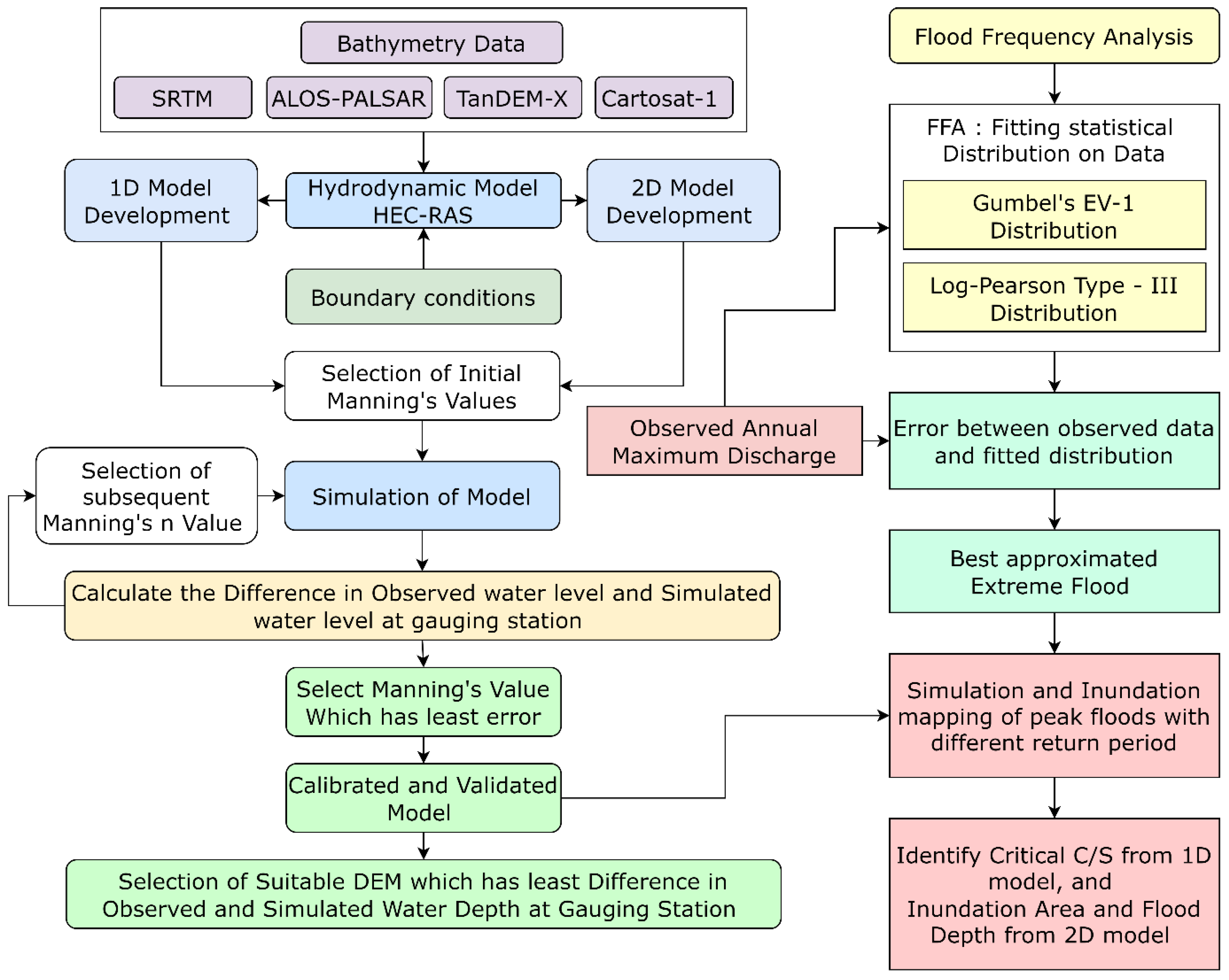
The required data for the present study, including DEMs, gauge and discharge data, and the Land-Use Land-Cover (LULC) map, were collected from various government organizations. The downstream stretch of the river, bounded by the Madhuban dam upstream and the Arabian Sea downstream, were considered the study area with four gauge stations, namely, Madhuban Dam, Silvassa, Vapi, and Daman (as shown in Figure 2). The hourly gauge and discharge data for the gauging station and dam site were obtained from the Central Water Commission (CWC, Surat) and Damanganga Project Circle (GPC, Valsad). The LULC map of the study region with a 30 m spatial resolution was developed from Landsat 8 satellite imagery using the maximum likelihood classification of ArcGIS v10.8. Four freely available DEMs were utilized for the present study, viz. SRTM DEM [31] of 30 m spatial resolution obtained from https://earthexplorer.usgs.gov/ (accessed on 15 March 2023), ALOS-PALSAR DEM [41] of 12.5 m spatial resolution obtained from https://asf.alaska.edu/ (accessed on 18 March 2023), TanDEM-X [42] of 90 m spatial resolution obtained from https://tandemx-science.dlr.de/ (accessed on 1 March 2023), and Cartosat-1 DEM [43] of 30 m spatial resolution obtained from https://bhuvan.nrsc.gov.in (accessed on 15 March 2023).

3. Methodology

The methodology includes data collection, pre-processing the datasets for flood modeling, flood frequency analysis using statistical methods, and developing hydrodynamic models for simulating flows along the river channel (1D HD model) and floodplains (2D HD model). The flow chart for the adopted methodology in the present study is shown in Figure 3.

3.1. One-Dimensional–Two-Dimensional Hydrodynamic Models Using HEC-RAS

In 1D HD modeling, it is presumable that the flow only changes direction longitudinally towards the downstream side. The study aimed to estimate the water depth, water surface elevation, and velocity profile at each 1D model cross-section. The longitudinal and lateral flows occur simultaneously in the 2D model. HEC-RAS software is used for 1D and 2D modeling. This software was developed by U. S. Army Corps of Engineers. HEC-RAS uses a four-point implicit finite difference scheme to determine the water surface profiles for a steady and gradually changing flow.
In the present study, HEC-RAS v6.3 was used to develop a 1D and 2D HD model for simulating the flood flows along the river and floodplains in the Damanganga basin. Using ArcGIS v10.8, the DEMs with different spatial resolutions were pre-processed to fill the sinks and eliminate peaks. Systematic errors occur when developing DEMs because the sinks and peaks have lower and higher cell values than the surrounding cells. In the 1D model, cross-sections were extracted from various DEMs, and for 2D modeling, the DEM, which produced the least error in the 1D model, was used as terrain data. For the 1D and 2D HD models, the four days of releases from the Madhuban dam for the flood events of 2016, 2011, and 2008 were considered the upstream boundary condition, and normal depth was considered the downstream boundary condition since there were no other tributaries that might influence the peak flows (as shown in Figure 2). Calibration and validation of the model were also carried out from the results obtained and subsequently by changing Manning’s and n values of the river channel (for 1D HD model) and different classes of LULC (for 2D HD model). For calibrating the 1D HD model, the global roughness coefficient was used, i.e., considering the single roughness value for the entire stretch of the riverbed. In reality, the riverbed characteristics may not be exactly the same for the entire length of riverbed. However, the changes in riverbed characteristics for the Damanganga River are not significant enough to require different Manning’s coefficients for different sections of the river. Furthermore, detailed riverbed survey data are not available for most of the Indian River basin, leading to data scarcity issues. Therefore, in the absence of detailed riverbed survey data, various studies have used a single Manning’s coefficient for the Indian River basin, including nearby basins [44,45]. The calibrated and validated model with the DEM that produced the least error was then used to simulate the peak floods corresponding to 10, 25, 50, and 100-years of return periods. The flood inundation maps were prepared by exporting the water depth layer from the RAS Mapper of HEC-RAS to ArcGIS v10.8.

3.2. Frequency Analysis of the Flood Flow

The GEV and LP-III statistical distribution were fitted to the maximum flow data of the Madhuban dam for the flood frequency analysis (FFA). In total, 30 years of data were used from 1990 to 2019 for the FFA.

3.2.1. Gumbel’s Extreme Value (GEV) Method

The peak annual flow data (x) were collected from 1990 to 2019 to fit the flow data distribution. Then, the mean ( x ¯ ) and standard deviation ( σ x) were calculated from the Peak discharge data for N years using the following formulas: x ¯ = i = 1 n x N and σ x = X X ¯ 2 N 1 . The reduced mean (Yn) and reduced standard deviation (Sn) were selected from Gumbel’s extreme value distribution table [46]. Then, the return periods (T) were calculated using the Weibull equation (Equation (1)) for each annual peak flood.
T = N + 1 m
where N is the number of years, and m is the rank assigned to the data after arranging them in descending order of magnitude. After, the flood magnitudes (XT) with different return periods were computed using Gumbel’s EV Distribution Equation (Equation (2)).
X T = X + K T σ x
where KT is the frequency factor which is expressed as Y T Y n S n , in which YT is the reduced variate calculated as Y T = ln ln T T 1 .

3.2.2. Log-Pearson Type III (LP-III) Method

The U.S. Water Resources Council adopted the LP-III distribution in 1967. First, the time series of logarithmic discharge value (x) was prepared. Then mean ( Z ¯ ) and standard deviation ( σ z) of the logarithmic discharge value was calculated using Z ¯ = l o g x N and σ z = Z Z ¯ 2 N 1 . Here, N is the number of years. The coefficient of skewness (Cs) was then calculated using Equation (3).
C s = N Z Z ¯ 3 N 1 N 2 σ z 3
The frequency factor for different return periods was obtained using the value of the coefficient of skewness from the frequency factor (Kz) table of the log-Pearson type III distribution [46]. Finally, the extreme values (ZT) were calculated for different return periods using Equation (4) and antilogarithmic ZT was used to obtain the peak discharge value for different return periods.
Z T = Z ¯ + K z σ z

4. Results and Discussion

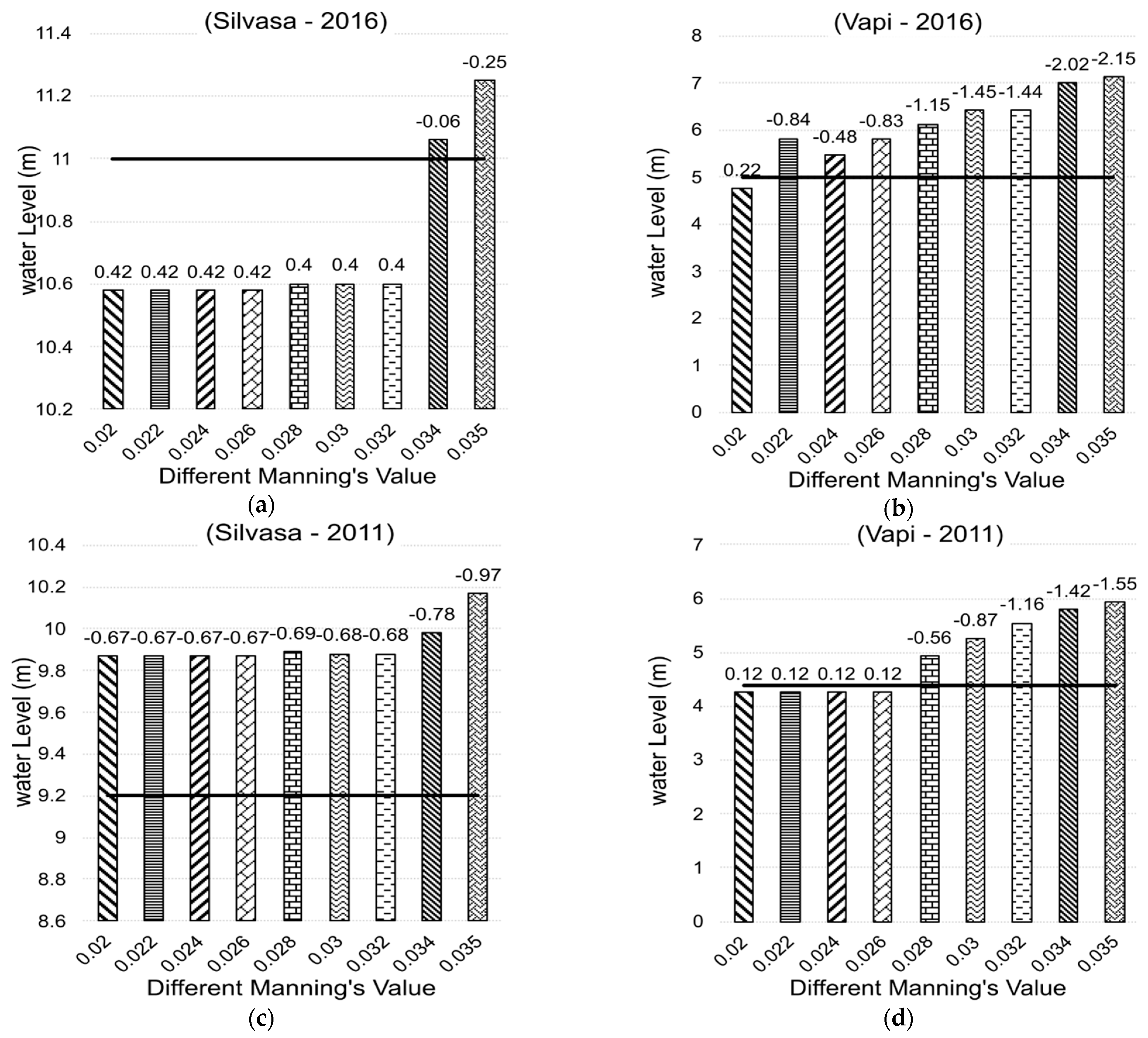
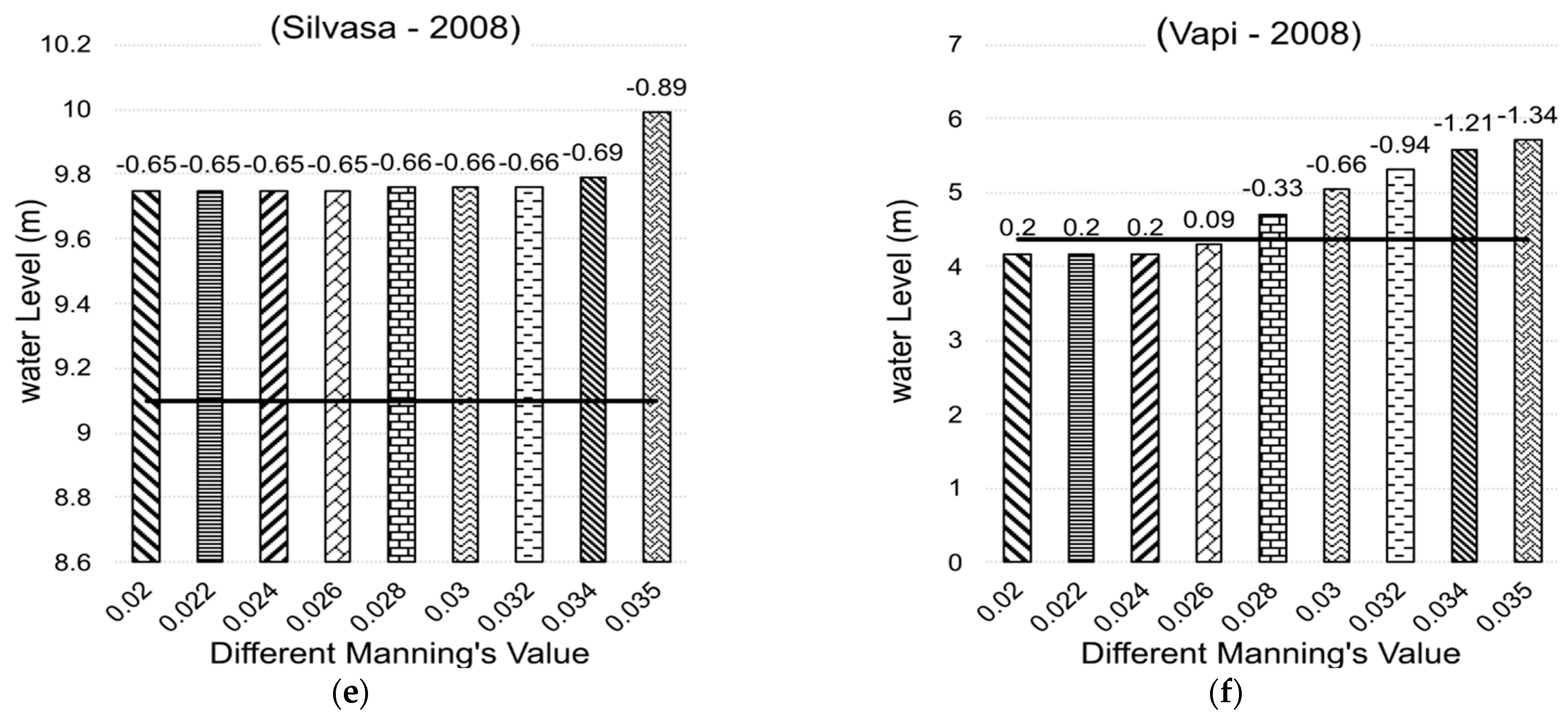
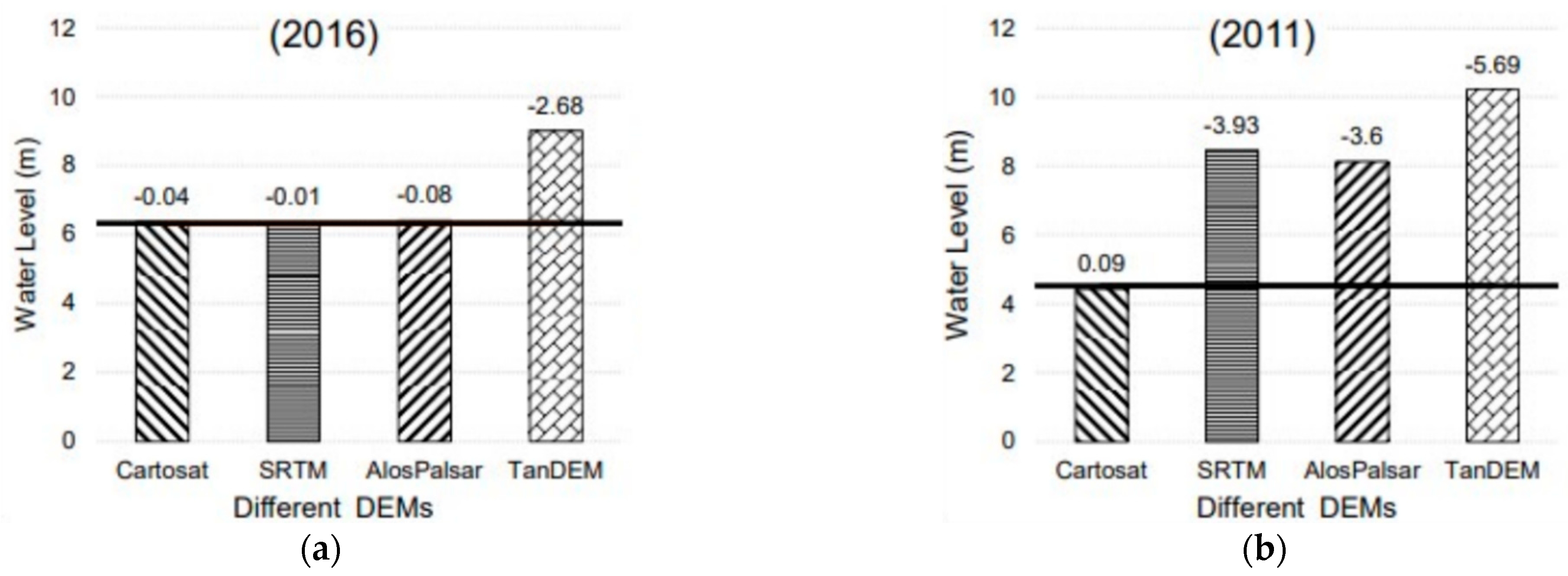
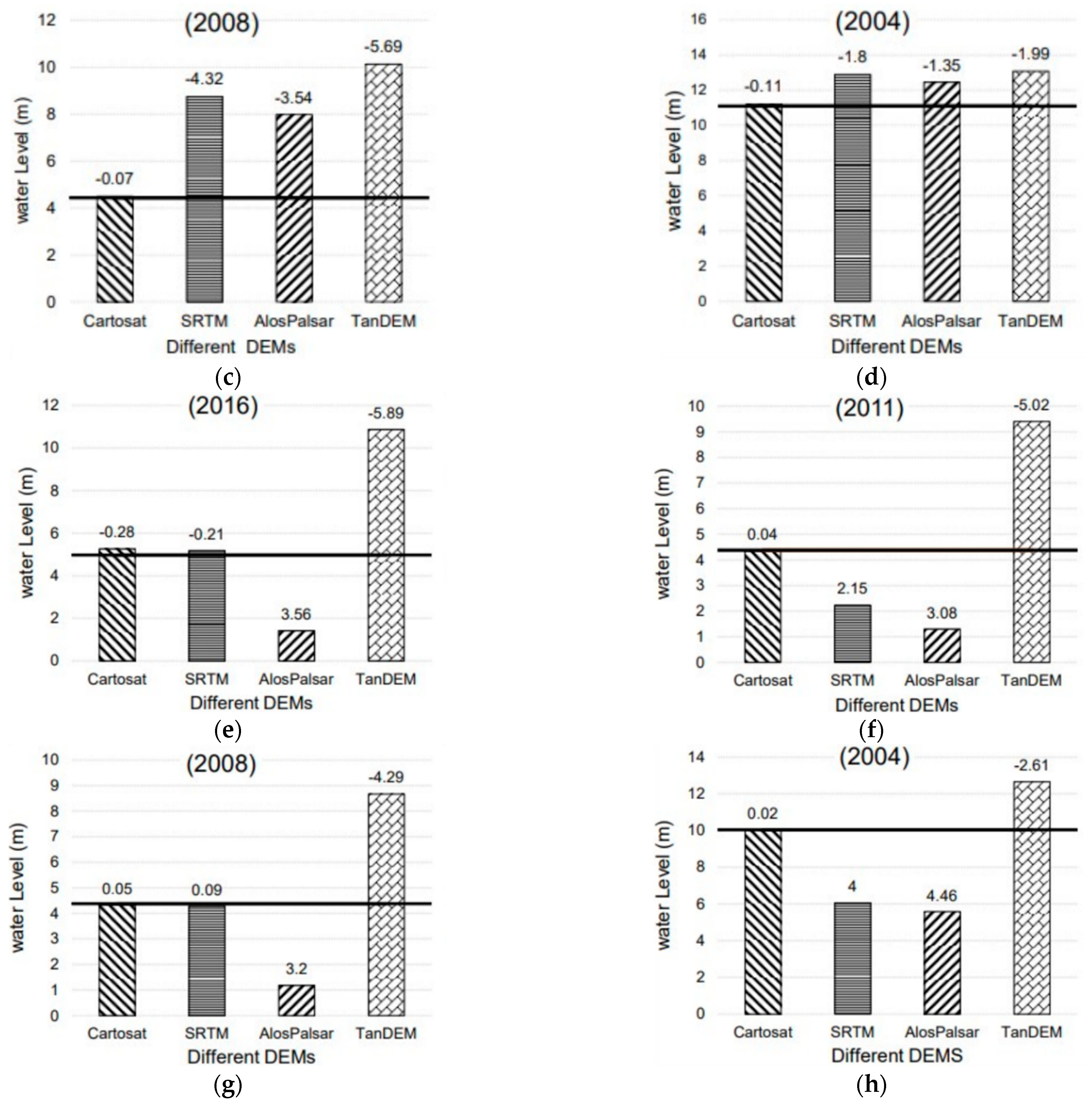
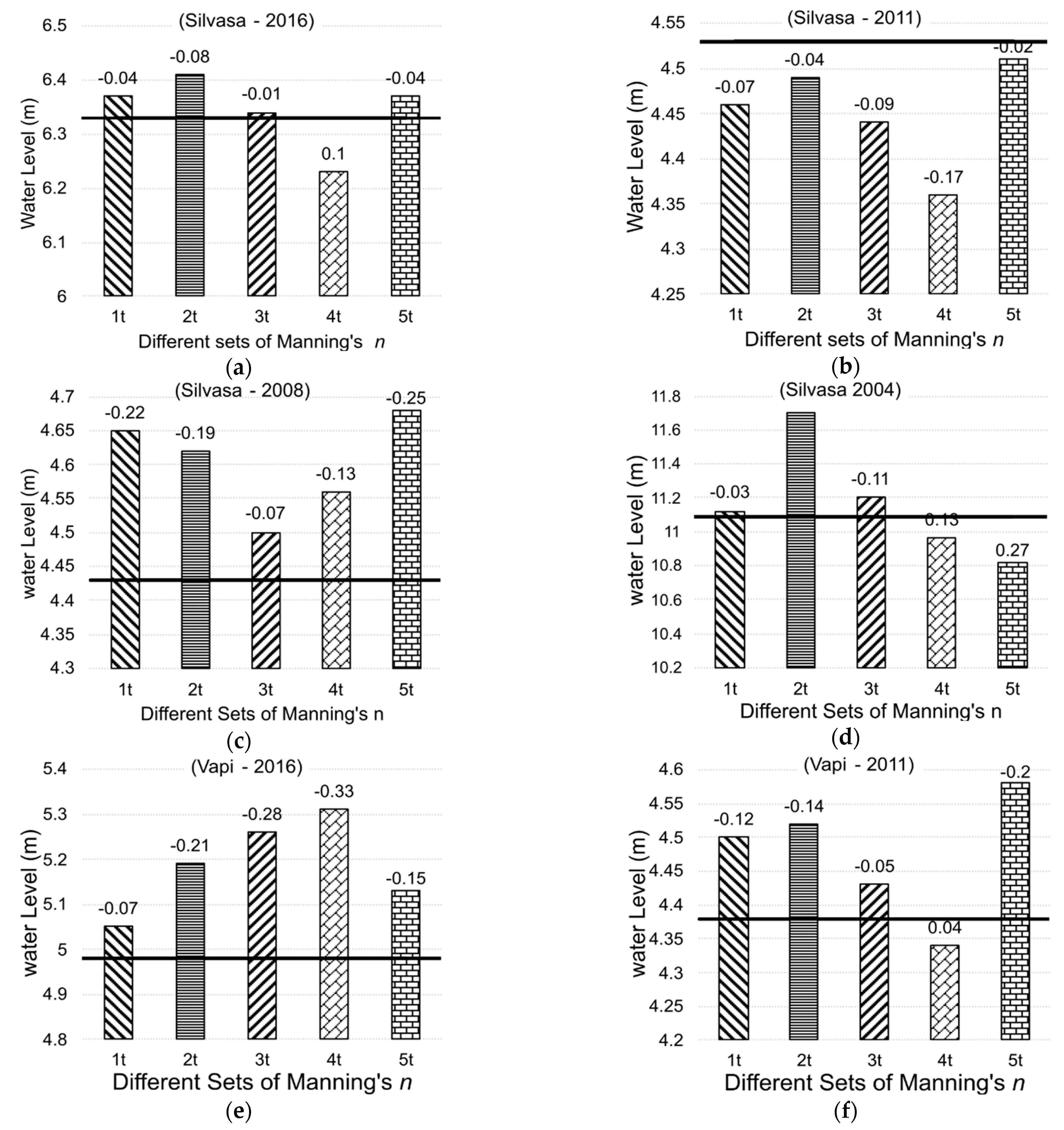
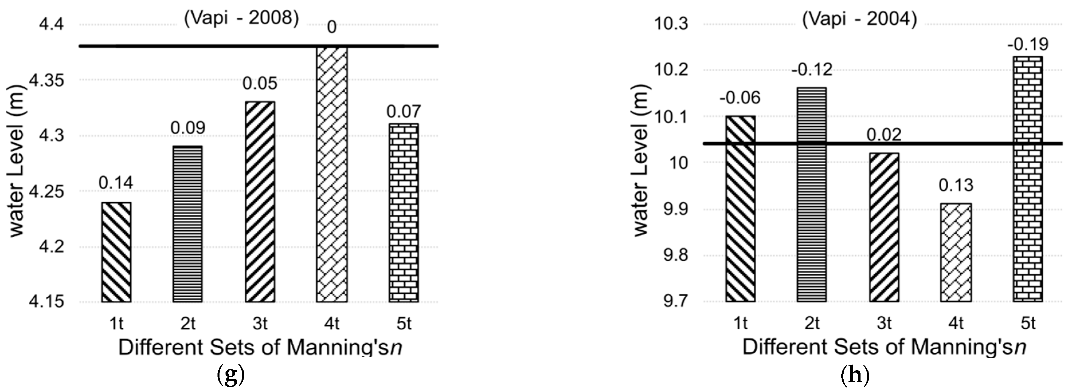
4.1. Evaluating Efficacy of Different DEMs for Hydrodynamic Modeling

At the Silvassa and Vapi gauging stations, the 1D model was calibrated and validated by adjusting the river’s roughness coefficient from 0.02 to 0.035 based on river characteristics [47]. Figure 4 (refer to subfigures Figure 4a–f) shows the results of the simulated models for the different Manning’s n values and actual water depth for the years 2016, 2011, and 2008 at the Silvassa and Vapi gauging station. The result indicates that for lower values of Manning’s and n, the difference between actual and simulated water levels is nearly the same. As Manning’s n value increases, the corresponding simulated water level increases. From these comparisons, Manning’s n value of 0.02, which gives an absolute minimum error, was selected as the calibrated n value for further analysis. This calibrated model was then used to simulate the flood events using different DEMs as input for the river bathymetry.
Figure 5 (refer to subfigures Figure 5a–h) shows the results of the simulated water level with different DEMs as input for the bathymetry data for the flood events of 2016, 2011, 2008, and 2004 at the Silvassa and Vapi gauge stations. The results indicate that the Cartosat-1 DEM is the most reliable for flood mapping in the Indian coastal floodplain compared to other globally freely available DEMs with different resolutions. It is perhaps obvious that higher resolution DEMs produce more accurate results as long as the model can handle such high-resolution DEMs. However, the results of this study indicate that ALOS-PALSAR DEM with 12.5 m resolution also failed to produce reliable results for different flood events in the Damanganga basin. Pathan et al. [29] have shown that SRTM DEM produces a reliable output for flood modeling in the Purna river basin, neighboring the Damanganga river Basin. This indicates that even in close proximity, the efficacy of DEM can be changed, and it is essential to evaluate all available datasets for producing reliable outputs. Based on these results, Manning’s n as 0.02 for the roughness coefficient of the river channel, and Cartosat-1 DEM for the input bathymetry of the model, were selected for simulating flood inundation and risk maps of the Damanganga basin.

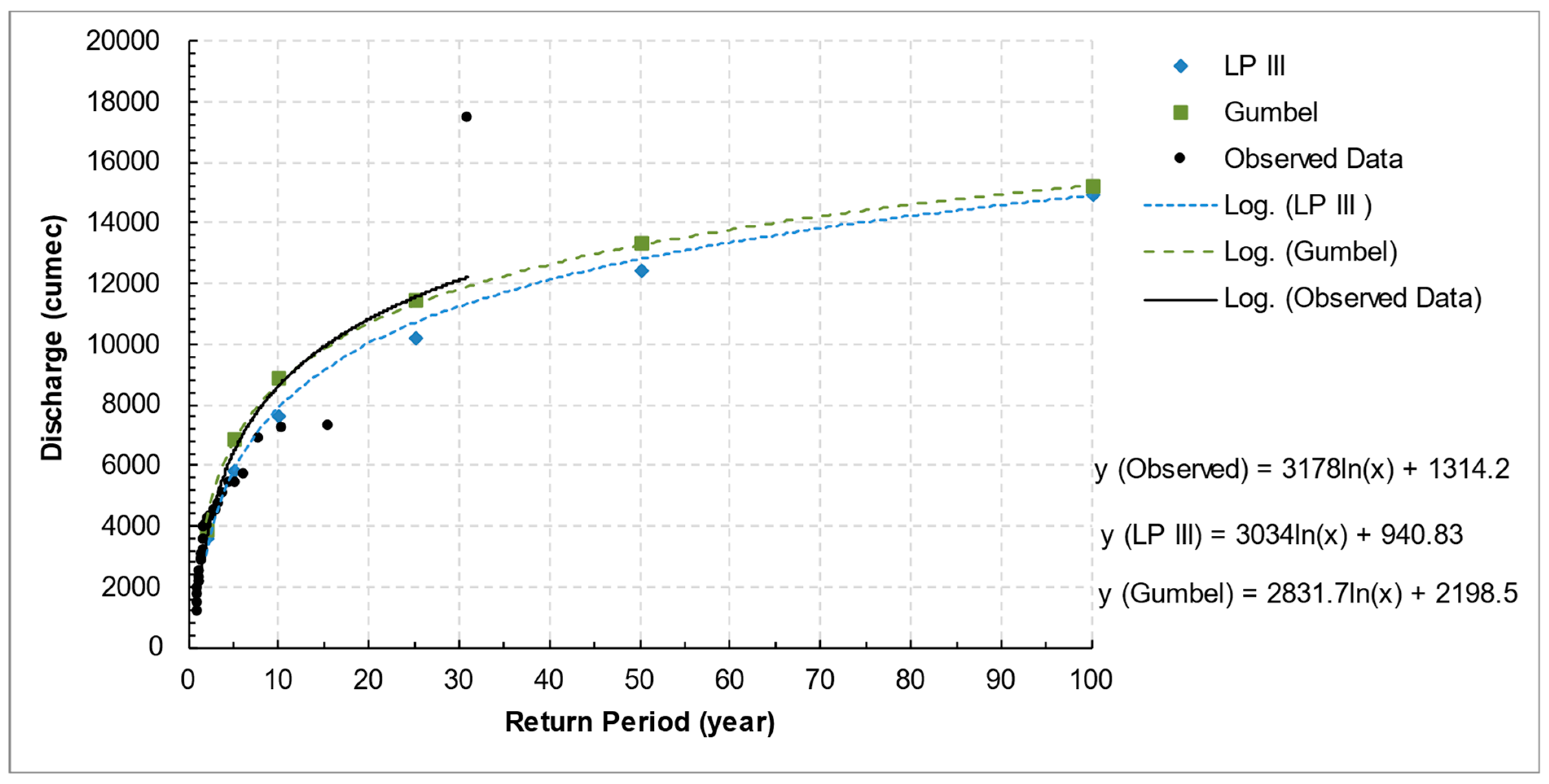
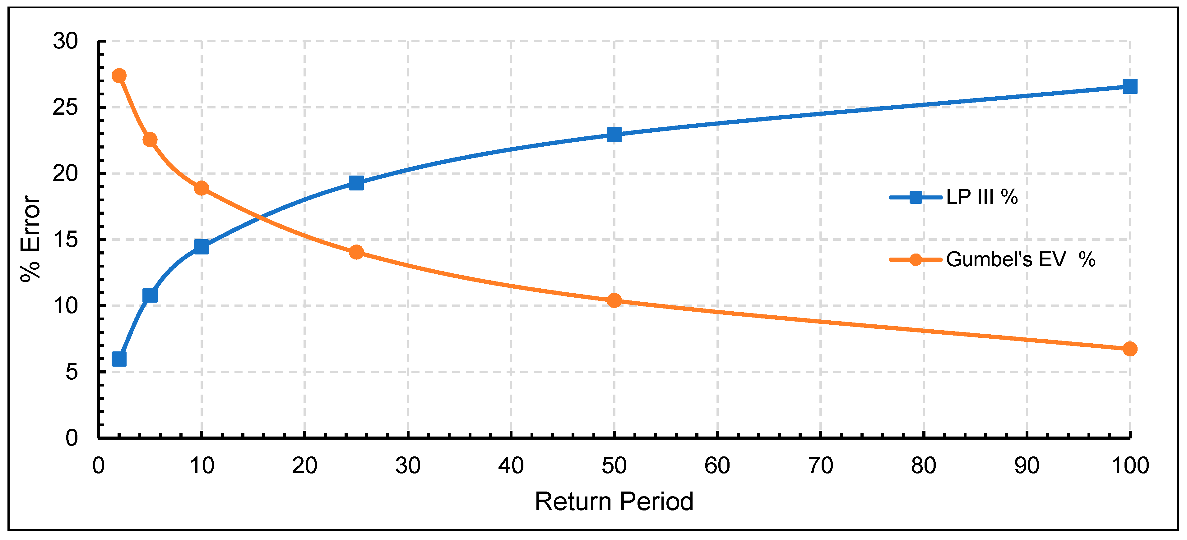
4.2. Results of Flood Frequency Analysis (FFA)

The mean and standard deviation for the GEV method were obtained for the peak discharge series. The required Yn and Sn values were calculated by the Weibull equation using Gumbel’s extreme value distribution table [46] and the return period (T). Gumbel’s distribution equation was then used to calculate the maximum discharge for different return periods. For the LP-III method, the logarithm values of the peak discharge series were considered. The standard deviation and mean of this series were then obtained. For the provided years, the coefficient of skewness was calculated. The frequency factor for different return periods was computed using the skewness coefficient value from the LP-III distribution’s frequency factor table [46]. The ZT value was calculated for each return period, and the antilog of ZT was obtained as the probable discharge value corresponding to different return periods. The estimated parameters of the GEV and LP-III distributions are shown in Table 1.
Table 2 shows the estimated extreme values of peak flood using GEV and LP-III methods for return periods of 10, 25, 50, and 100 years, respectively.
The result indicates the significant difference between the estimated flood from the GEV and LP-III distribution methods. To evaluate the reliability of these results, the fitted distribution from both methods was compared with the observed data, as shown in Figure 6. The percentage error between the fitted results of the GEV and LP-III and the observed data revealed that the LP-III method provides more accurate results for lower return period floods up to 15 years, and for higher return period floods, the GEV method provides more reliable estimation (Figure 7). These results are consistent with the previous studies [48]. Based on the results from both methods, the probable flood estimates of a 10-year return period from the LP-III method and 25-, 50-, and 100-year return periods from the GEV method were considered for generating flood inundation and risk maps.

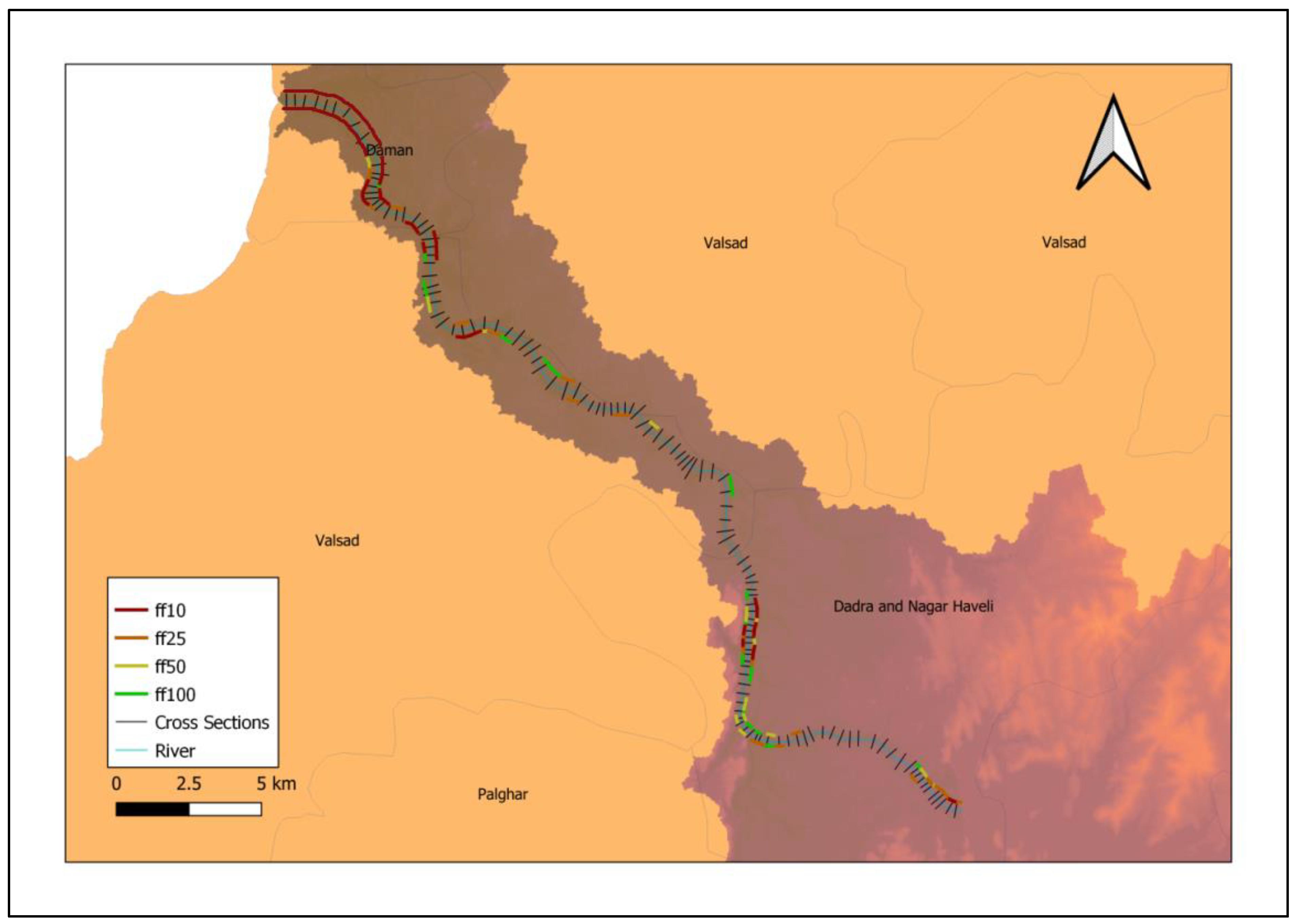
4.3. Mapping of Flood Risk River Sections

Flood risk refers to the possibility of flooding as well as its potential negative effects. In this study, the critical cross-section and river reach were identified based on the obtained results of the 1D HD model. The flood risk level at a particular cross-section was decided based on overtopping water depth for the different return periods of floods and surrounding land use. For example, the cross-section which overflows even with the 2-year return period flood and has urban land cover nearby is marked as a high-risk cross-section. Figure 8 shows the overtopping cross-section map corresponding to return periods of 10, 25, 50, and 100 years. To mark the overtopping cross-sections, the geometry data files from HEC-RAS were exported in GIS format, and then the flood risk at particular cross-sections was identified based on the overtopping water depth and surrounding land-use classification. The red line in Figure 8 indicates the very high-risk river reach where cross-sections do not have sufficient width and depth to carry the 10-year return period floods. The orange and yellow markings indicate the high- and moderate-risk sections, which are overflowing with 25–50-year return period floods and have urban land cover in the surrounding area. The green marking indicates the low-risk sections, which are overflowing, but the surrounding areas are less vulnerable. These critical cross-section maps can be helpful in the prioritization of the location for the construction of the levee to mitigate the flood risk in the Damanganga basin.

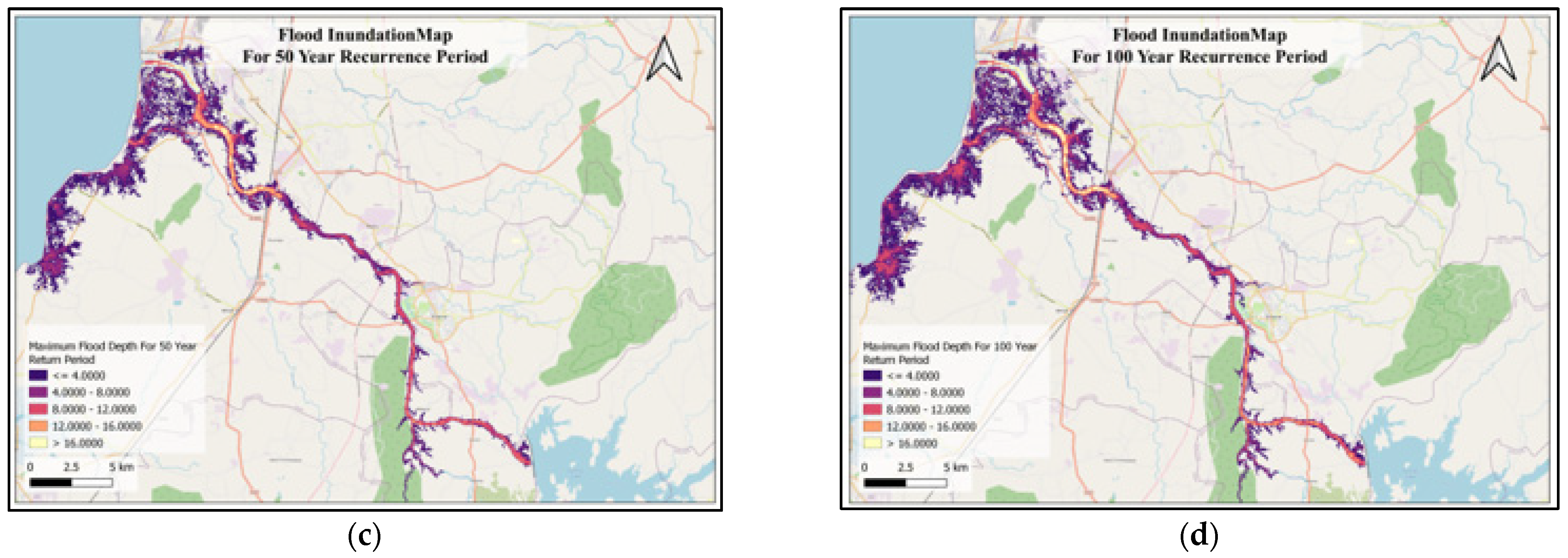
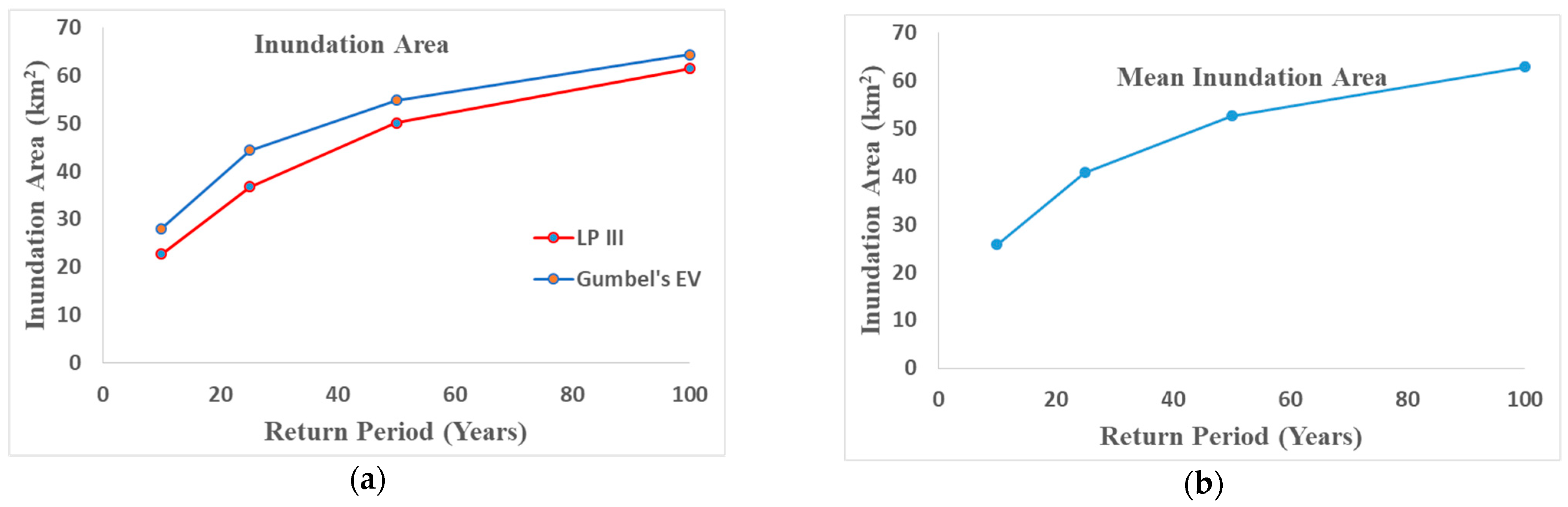
4.4. Mapping of Flood Inundation and Risk Areas in Floodplain

The flood inundation map corresponding to different return period floods was prepared using the 2D HD model by calibrating the model for the different Manning’s n values of the floodplain. Different sets of Manning’s n values corresponding to different LULC classes [47,49] were given as input to the model (Table 3), and the simulated water depths were compared with the actual water depth to compute the absolute errors.
From the visual inspection of the land-use land cover of the basin, we found that most of the basin area is covered with cropland and built-up area. For the calibration of the 2D model, we manually optimized Manning’s n values for different LULC categories by trial and error, i.e., t1 in Table 3 represents the values of Manning’s n for different LULC categories considered for trial 1. We calibrated the model by manually adjusting the roughness coefficient value for the cropland and build-up area in a specified range and keeping it almost constant for the other LULC category. To determine the optimized roughness coefficient values, the simulated water levels were compared with the observed water levels at two-gauge stations where observed water level data were available (as shown in Figure 9a–h). Since the observed water level data were not available for the floodplain, we conducted a questionnaire survey to obtain the actual flood depth data at a few essential points to validate the simulated results. Figure 9 (refer to subfigures Figure 9a–h) shows the water level graphs at the gauge site; horizontal lines show the actual flood depth, and the calculated absolute error at the Silvasa and Vapi gauging stations is written on the bars of different sets of Manning’s n. Based on these results, the 3t (3rd trial) set of Manning’s n values (refer to Table 3), which gives a comparatively lower absolute error, was selected as the final Manning’s n value for the floodplain. This calibrated and validated model was then used to simulate the estimated peak flood for different return periods.
Figure 10 (refer to subfigures Figure 10a–d) shows the inundation maps for the 10-, 25-, 50-, and 100-year return period floods corresponding to the best estimates from the FFA. Overall, the flood inundation maps show that the basin’s lower region is at higher flood risk, and Daman and Bilad regions are most affected by different return period floods. The inundation areas for the 10-, 25-, 50-, and 100-year return period floods are 22.86, 44.76, 54.86, and 64.56 km2, respectively. However, the probabilistic nature of the GEV and LP-III methods may have generated some uncertainty in the estimated flood peak of different periods. To incorporate the uncertainty from the input data and probabilistic results of FFA, the ±5% band was added to the results with the hypothesis that it may incorporate the resulting error.
As shown in Figure 11 (refer to subfigures Figure 11a,b), the GEV method gave a comparatively higher estimate than the LP-III method. The mean inundation area corresponding to the peak flood estimated from the GEV and LP-III method is also shown in Figure 11, with the upper bound as the GEV and the lower bound as the LP-III method results. The difference between the mean inundation areas of different return period floods shows the higher uncertainty in the 25-year return period floods and the lowest uncertainty in 100-year return period floods. These simulated inundation maps and flood risk areas would be helpful to government authorities in prioritizing flood mitigation measures and relief measurements.

4.5. Climate Change and Importance of Flood Modeling

Recent flash floods in many countries showcase the direct impact of climate change on the hydrological cycle. Some countries are experiencing having higher and more intensified rainfalls [50,51,52,53] while some other countries are experiencing droughts [54,55,56,57] due to ongoing climate change. Each scenario is harmful or causes many adverse impacts on livelihood. Therefore, proper planning is essential to minimize the impacts. However, adaptation to the changing climate is highly necessary for reaching sustainable goals. For example, identifying crops that can be adapted to the changing climate to achieve better harvests is highly important in feeding the world. Similarly, adaptation to floods due to climate change is one of the most important sectors which people have to think of while looking at any mitigation options.
Floods are always disastrous, and thus cause significant damage not only to properties but also to lives. Therefore, flood prediction in the extreme events of climate change is one adaptation strategy that the world is using for essential planning purposes. However, the accuracy of the prediction is still doubtful due to the higher unpredictability of climate scenarios. Recent technological advances are enhancing predictability; however, most floods are still causing damage. Therefore, evaluating the efficacy of DEMs in flood modeling requires more attention to climate change. Land use changes on top of the changing climate worsen the mitigation strategies. However, a common platform is necessary to address the efficacy of DEMs to predict more accurate flood scenarios under climate change. In addition, the locality is important as the characteristics of the DEMs are different from one location to another. Therefore, this research addresses the identified research gap related to climate change.

4.6. Limitations and Future Scope of the Study

In the present study, the uncertainty associated with the DEM was analyzed for hydraulic modeling and flood inundation mapping. However, the uncertainty associated with the input data, model parameters, and model simulation was not considered which can thus be considered as a limitation for the study. The uncertainty in the input data can be caused by instrumentation error (in case of gauge measurement) or model structural errors (in case of satellite-based dataset). The future work can analyze the uncertainty associated with the developed flood inundation map for enhancing the results. The model parameters are an important factor which can cause the uncertainty in the outcomes and are required to be taken care of. For the present study, the HEC-RAS model was used for flood inundation mapping. Many sources of uncertainty affect the hydraulic modeling processes and several studies have already addressed this issue. In this project, we are focusing on the inputs of the model, namely the measured inflows and estimated lateral inflows, as well as the roughness coefficients. The water in HEC-RAS modeling has been assumed to flow in the longitudinal direction only, i.e., the flow is one-dimensional, implying that there is no direct modeling of the hydraulic effects of the cross-section shape changes, bends, and other two and three-dimensional aspects of flow. It represents the terrain as a sequence of cross-sections and simulate flow to estimate the average velocity and water depth at each cross-section. The uncertainties associated with the breach parameters, especially breach width, breach depth, and breach development time, may cause uncertainty in flood peak and arrival time. Further, the high velocity flows associated with dam break floods can cause significant scouring of channels.

5. Summary and Conclusions

In the present study, the efficacy of four open-source DEMs for flood modeling, viz. SRTM 30 m, ALOS-PALSAR 12.5 m, TanDEM-X 90m, and Cartosat-1 30 m, was evaluated by one-dimensional (1D) and two-dimensional (2D) hydrodynamic (HD) models using HEC-RAS v6.3 for the Damanganga river basin. Manning’s roughness coefficient value of 0.02 was calibrated using the 1D HD model for the riverbed. Then, the calibrated and validated model was used with different DEMs as input bathymetry data to evaluate the efficacy of DEMs in the flood model. The results showed that Cartosat-1 DEM with a 30 m spatial resolution produced more reliable results than others for the Damanganga basin, which nullifies the hypothesis that high-resolution DEMs can have the most accurate bathymetry of the river, as the ALOS-PALSAR DEM with a 12.5 m spatial resolution also failed to produce reliable results. Based on these results, the calibrated values of the roughness coefficient for the river bathymetry as 0.02 and Cartosat-1 DEM as the bathymetry data for the model were chosen for further study. To find the appropriate method, the comparison was made for the estimated peak floods for 10-, 25-, 50-, and 100-year return periods from the GEV and LP-III methods with the observed streamflow, which indicates that the LP-III method gives more reliable peak flood estimates up to a period of 15 years of return and the GEV method gives more reliable estimates for higher return period floods. It suggests that the LP-III method is more suitable for the short-term flood frequency analysis, and the GEV method is more suitable for the long-term flood frequency analysis. The calibrated and validated 1D and 2D HD models were then used to simulate the estimated peak floods for different return periods. The critical river reach sections were identified based on overflowing cross-sections from the 1D simulation and population in the surrounding areas, indicating that the basin’s lower area is at a high flood risk. The inundation maps from the 2D HD model show that the Daman and Bhilad region in the lower part of the basin, including the coastal area, is at a higher risk of flooding. An area of approximately 64.56 km2 was inundated in the flood of the year 2004 with a maximum flood depth of 9.03 m and maximum velocity of 1.2 m s−1. The inundation area corresponding to 10-, 25-, 50-, and 100-year return period floods was approximately 22.86, 44.76, 54.86, and 64.56 km2, respectively. Future floods can be prevented, and the city’s susceptibility to flooding events can be directly improved using the FFA calculations, flood inundation maps, and identified critical river reach sections.

Author Contributions

Conceptualization, D.J.M. and U.R.; methodology, P.G.; software, N.K.M.; validation, D.J.M.; formal analysis, P.G.; investigation, P.G.; resources, N.K.M.; data curation, P.G.; writing—original draft preparation, P.G. and D.J.M.; writing—review and editing, N.M. and U.R.; visualization, P.G.; supervision, D.J.M.; project administration, D.J.M., N.M. and U.R. All authors have read and agreed to the published version of the manuscript.

Funding

This research received no external funding.

Data Availability Statement

Data used in this research are only available for research purposes from the corresponding author.

Conflicts of Interest

The authors declare no conflict of interest.

References

  1. Mangukiya, N.K.; Sharma, A. Flood risk mapping for the lower Narmada basin in India: A machine learning and IoT-based framework. Nat. Hazards 2022, 113, 1285–1304. [Google Scholar] [CrossRef]
  2. Tanoue, M.; Hirabayashi, Y.; Ikeuchi, H. Global-scale river flood vulnerability in the last 50 years. Sci. Rep. 2016, 6, 36021. [Google Scholar] [CrossRef] [PubMed]
  3. Dash, P.; Punia, M. Governance and disaster: Analysis of land use policy with reference to Uttarakhand flood 2013, India. Int. J. Disaster Risk Reduct. 2019, 36, 101090. [Google Scholar] [CrossRef]
  4. Huong, H.T.L.; Pathirana, A. Urbanization and climate change impacts on future urban flooding in Can Tho city, Vietnam. Hydrol. Earth Syst. Sci. 2013, 17, 379–394. [Google Scholar] [CrossRef]
  5. Mohanty, M.P.; Mudgil, S.; Karmakar, S. Flood management in India: A focussed review on the current status and future challenges. Int. J. Disaster Risk Reduct. 2020, 49, 101660. [Google Scholar] [CrossRef]
  6. Mohapatra, P.K.; Singh, R.D. Flood Management in India. Nat. Hazards 2003, 28, 131–143. [Google Scholar] [CrossRef]
  7. Nanditha, J.; Mishra, V. On the need of ensemble flood forecast in India. Water Secur. 2021, 12, 100086. [Google Scholar] [CrossRef]
  8. National Institution for Transforming India (NITI). Report of the Committee Constituted for Formulation of Strategy for Flood Management Works in Entire Country and River Management Activities and Works Related to Border Areas (2021–2026); NITI: New Delhi, India, 2021; 120p. Available online: https://www.preventionweb.net/publication/report-committee-constituted-formulation-strategy-flood-management-works-entire-country (accessed on 12 February 2023).
  9. National Institute of Disaster Management (NIDM). Hydro-Meteorological Disasters Characteristics of Flood; NIDM: New Delhi, India, 2007; pp. 1–46. Available online: https://nidm.gov.in/PDF/Disaster_hymet.pdf (accessed on 12 February 2023).
  10. Singh, R.D. Real-Time flood Forecasting: Indian Experience. In Hydrological Modelling in Arid and Semi-Arid Areas; Wheater, H., Sorooshian, S., Sharma, K.D., Eds.; Cambridge University Press: Cambridge, UK, 2007; pp. 139–156. ISBN 9780521869. [Google Scholar] [CrossRef]
  11. Tripathi, P. Flood Disaster in India: An Analysis of trend and Preparedness. Interdiscip. J. Contemp. Res. 2015, 2, 91–98. [Google Scholar]
  12. Yadav, S.M.; Mangukiya, N.K. Semi-arid River Basin Flood: Causes, Damages, and Measures. In Proceedings of the Fifth International Conference in Ocean Engineering (ICOE2019); Sundar, V., Sannasiraj, S.A., Sriram, V., Nowbuth, M.D., Eds.; Lecture Notes in Civil Engineering; Springer: Singapore, 2021; Volume 106, pp. 201–212. [Google Scholar] [CrossRef]
  13. Lim, N.; Brandt, S. Flood map boundary sensitivity due to combined effects of DEM resolution and roughness in relation to model performance. Geomat. Nat. Hazards Risk 2019, 10, 1613–1647. [Google Scholar] [CrossRef]
  14. Whipple, A.A.; Viers, J.H.; Dahlke, H.E. Flood regime typology for floodplain ecosystem management as applied to the unregulated Cosumnes River of California, United States. Ecohydrology 2017, 10, e1817. [Google Scholar] [CrossRef]
  15. Abdrabo, K.I.; Kantoush, S.A.; Saber, M.; Sumi, T.; Habiba, O.M.; Elleithy, D.; Elboshy, B. Integrated Methodology for Urban Flood Risk Mapping at the Microscale in Ungauged Regions: A Case Study of Hurghada, Egypt. Remote Sens. 2020, 12, 3548. [Google Scholar] [CrossRef]
  16. Mangukiya, N.K.; Yadav, S.M. Integrating 1D and 2D hydrodynamic models for semi-arid river basin flood simulation. Int. J. Hydrol. Sci. Technol. 2022, 14, 206–228. [Google Scholar] [CrossRef]
  17. Mehta, D.J.; Yadav, S.M. Hydrodynamic Simulation of River Ambica for Riverbed Assessment: A Case Study of Navsari Region. Lect. Notes Civ. Eng. 2020, 39, 127–140. [Google Scholar] [CrossRef]
  18. Mehta, D.J.; Eslamian, S.; Prajapati, K. Flood modelling for a data-scare semi-arid region using 1-D hydrodynamic model: A case study of navsari region. Model. Earth Syst. Environ. 2021, 8, 2675–2685. [Google Scholar] [CrossRef]
  19. Pramanik, N.; Panda, R.K.; Sen, D. One Dimensional Hydrodynamic Modeling of River Flow Using DEM Extracted River Cross-sections. Water Resour. Manag. 2010, 24, 835–852. [Google Scholar] [CrossRef]
  20. Shustikova, I.; Domeneghetti, A.; Neal, J.C.; Bates, P.; Castellarin, A. Comparing 2D capabilities of HEC-RAS and LISFLOOD-FP on complex topography. Hydrol. Sci. J. 2019, 64, 1769–1782. [Google Scholar] [CrossRef]
  21. Timbadiya, P.V.; Patel, P.L.; Porey, P.D. Hec-Ras Based Hydrodynamic Model in Prediction of Stages of Lower Tapi River. ISH J. Hydraul. Eng. 2011, 17, 110–117. [Google Scholar] [CrossRef]
  22. Timbadiya, P.V.; Patel, P.L.; Porey, P.D. A 1D–2D Coupled Hydrodynamic Model for River Flood Prediction in a Coastal Urban Floodplain. J. Hydrol. Eng. 2015, 20, 05014017. [Google Scholar] [CrossRef]
  23. Bales, J.; Wagner, C. Sources of uncertainty in flood inundation maps. J. Flood Risk Manag. 2009, 2, 139–147. [Google Scholar] [CrossRef]
  24. Beven, K.; Lamb, R.; Leedal, D.; Hunter, N. Communicating uncertainty in flood inundation mapping: A case study. Int. J. River Basin Manag. 2015, 13, 285–295. [Google Scholar] [CrossRef]
  25. Bellos, V.; Kourtis, I.M.; Moreno-Rodenas, A.; Tsihrintzis, V.A. Quantifying Roughness Coefficient Uncertainty in Urban Flooding Simulations through a Simplified Methodology. Water 2017, 9, 944. [Google Scholar] [CrossRef]
  26. Khojeh, S.; Ataie-Ashtiani, B.; Hosseini, S.M. Effect of DEM resolution in flood modeling: A case study of Gorganrood River, Northeastern Iran. Nat. Hazards 2022, 112, 2673–2693. [Google Scholar] [CrossRef]
  27. Muthusamy, M.; Casado, M.R.; Butler, D.; Leinster, P. Understanding the effects of Digital Elevation Model resolution in urban fluvial flood modelling. J. Hydrol. 2021, 596, 126088. [Google Scholar] [CrossRef]
  28. Papaioannou, G.; Vasiliades, L.; Loukas, A.; Aronica, G.T. Probabilistic flood inundation mapping at ungauged streams due to roughness coefficient uncertainty in hydraulic modelling. Adv. Geosci. 2017, 44, 23–34. [Google Scholar] [CrossRef]
  29. Pathan, A.I.; Agnihotri, P.G.; Eslamian, S.; Patel, D. Comparative analysis of 1D hydrodynamic flood model using globally available DEMs—A case of the coastal region. Int. J. Hydrol. Sci. Technol. 2022, 13, 92. [Google Scholar] [CrossRef]
  30. Wohl, E.E. Uncertainty in Flood Estimates Associated with Roughness Coefficient. J. Hydraul. Eng. 1998, 124, 219–223. [Google Scholar] [CrossRef]
  31. Farr, T.G.; Rosen, P.A.; Caro, E.; Crippen, R.; Duren, R.; Hensley, S.; Kobrick, M.; Paller, M.; Rodriguez, E.; Roth, L.; et al. The Shuttle Radar Topography Mission. Rev. Geophys. 2007, 45, RG2004. [Google Scholar] [CrossRef]
  32. Samarasinghe, J.T.; Basnayaka, V.; Gunathilake, M.B.; Azamathulla, H.M.; Rathnayake, U. Comparing combined 1D/2d and 2D hydraulic simulations using high-resolution topographic data: Examples from Sri Lanka—Lower kelani river basin. Hydrology 2022, 9, 39. [Google Scholar] [CrossRef]
  33. Muhadi, N.A.; Abdullah, A.F.; Bejo, S.K.; Mahadi, M.R.; Mijic, A. The Use of LiDAR-Derived DEM in Flood Applications: A Review. Remote Sens. 2020, 12, 2308. [Google Scholar] [CrossRef]
  34. Brandt, S.A. Modeling and visualizing uncertainties of flood boundary delineation: Algorithm for slope and DEM resolution dependencies of 1D hydraulic models. Stoch. Environ. Res. Risk Assess. 2016, 30, 1677–1690. [Google Scholar] [CrossRef]
  35. McClean, F.; Dawson, R.; Kilsby, C. Implications of Using Global Digital Elevation Models for Flood Risk Analysis in Cities. Water Resour. Res. 2020, 56, e2020WR028241. [Google Scholar] [CrossRef]
  36. Li, J.; Wong, D.W. Effects of DEM sources on hydrologic applications. Comput. Environ. Urban Syst. 2010, 34, 251–261. [Google Scholar] [CrossRef]
  37. Brunner, G. HEC-RAS river Analysis System, Hydraulic Reference Manual, Version 4.1; Technical Report; US Army Corps of Engineers Hydrologic Engineering Center: Davis, CA, USA, 2010.
  38. Gumbel, E.J. The Return Period of Flood Flows. Ann. Math. Stat. 1941, 12, 163–190. [Google Scholar] [CrossRef]
  39. Hoshi, K.; Stedinger, J.R.; Burges, S.J. Estimation of log-normal quantiles: Monte Carlo results and first-order approximations. J. Hydrol. 1984, 71, 1–30. [Google Scholar] [CrossRef]
  40. Phien, H.N.; Ajirajah, T.J. Applications of the log Pearson type-3 distribution in hydrology. J. Hydrol. 1984, 73, 359–372. [Google Scholar] [CrossRef]
  41. Distributed Active Archive Center. ALOS PALSAR—Radiometric Terrain Correction, PALSAR_Radiometric_Terrain_Corrected_high_res. 2015. Available online: https://asf.alaska.edu/data-sets/derived-data-sets/alos-palsar-rtc/alos-palsar-radiometric-terrain-correction/ (accessed on 12 February 2023). [CrossRef]
  42. German Aerospace Center (DLR). TanDEM-X—Digital Elevation Model (DEM)—Global, 90m; German Aerospace Center (DLR): Oberpfaffenhofen, Germany, 2018. [Google Scholar] [CrossRef]
  43. CartoDEM Project. Augmented Stereo Strip Triangulation (ASST) Software Analysis Architecture Document—Report SAC/RESIPA/SIPG/CARTODEM/TN-01/February; Space Application Centre (ISRO): Ahmedabad, India, 2008.
  44. Pathan, A.I.; Agnihotri, P.G. Application of new HEC-RAS version 5 for 1D hydrodynamic flood modeling with special reference through geospatial techniques: A case of River Purna at Navsari, Gujarat, India. Model. Earth Syst. Environ. 2021, 7, 1133–1144. [Google Scholar] [CrossRef]
  45. Pathan, A.I.; Agnihotri, P.G.; Patel, D.; Prieto, C. Identifying the efficacy of tidal waves on flood assessment study—A case of coastal urban flooding. Arab. J. Geosci. 2021, 14, 2132. [Google Scholar] [CrossRef]
  46. Subramanya, K. Engineering Hydrology, 4th ed.; Tata McGraw-Hill Education: New York, NY, USA, 2013. [Google Scholar]
  47. Chow, V.T. Open-Channel Hydraulics; McGraw-Hill: New York, NY, USA, 1959. [Google Scholar]
  48. Mangukiya, N.K.; Mehta, D.J.; Jariwala, R. Flood frequency analysis and inundation mapping for lower Narmada basin, India. Water Pract. Technol. 2022, 17, 612–622. [Google Scholar] [CrossRef]
  49. Asante, K.O.; Artan, G.A.; Pervez, S.; Bandaragoda, C.; Verdin, J.P. Technical Manual for the Geospatial Stream Flow Model (GeoSFM). World Wide Web 2008, 605, 594–6151. [Google Scholar] [CrossRef]
  50. Gunathilake, M.B.; Amaratunga, Y.V.; Perera, A.; Chathuranika, I.M.; Gunathilake, A.S.; Rathnayake, U. Evaluation of future climate and potential impact on streamflow in the Upper Nan River basin of Northern Thailand. Adv. Meteorol. 2020, 2020, 8881118. [Google Scholar] [CrossRef]
  51. Emmanouil, S.; Langousis, A.; Nikolopoulos, E.I.; Anagnostou, E.N. Exploring the Future of Rainfall Extremes over CONUS: The Effects of High Emission Climate Change Trajectories on the Intensity and Frequency of Rare Precipitation Events. Earths Future 2023, 11, e2022EF003039. [Google Scholar] [CrossRef]
  52. Lei, C.; Yu, Z.; Sun, X.; Wang, Y.; Yuan, J.; Wang, Q.; Han, L.; Xu, Y. Urbanization effects on intensifying extreme precipitation in the rapidly urbanized Tai Lake Plain in East China. Urban Clim. 2023, 47, 101399. [Google Scholar] [CrossRef]
  53. Tamm, O.; Saaremäe, E.; Rahkema, K.; Jaagus, J.; Tamm, T. The intensification of short-duration rainfall extremes due to climate change—Need for a frequent update of intensity–duration–frequency curves. Clim. Serv. 2023, 30, 100349. [Google Scholar] [CrossRef]
  54. Qiu, J.; Shen, Z.; Xie, H. Drought impacts on hydrology and water quality under climate change. Sci. Total Environ. 2023, 858, 159854. [Google Scholar] [CrossRef]
  55. Ogunrinde, A.T.; Oguntunde, P.G.; Akinwumiju, A.S.; Fasinmirin, J.T.; Adawa, I.S.; Ajayi, T.A. Effects of climate change and drought attributes in Nigeria based on RCP 8.5 climate scenario. Phys. Chem. Earth Parts A/B/C 2023, 129, 103339. [Google Scholar] [CrossRef]
  56. Rusca, M.; Savelli, E.; Di Baldassarre, G.; Biza, A.; Messori, G. Unprecedented droughts are expected to exacerbate urban inequalities in Southern Africa. Nat. Clim. Chang. 2022, 13, 98–105. [Google Scholar] [CrossRef]
  57. Sahana, V.; Mondal, A. Evolution of multivariate drought hazard, vulnerability and risk in India under climate change. Nat. Hazards Earth Syst. Sci. 2023, 23, 623–641. [Google Scholar] [CrossRef]
Figure 1. Location map of the Damanganga river basin and topography obtained from different DEMs.
Climate 11 00114 g001
Figure 2. Locations of the Damanganga River gauge stations and cross-sections that are considered for the present study.
Climate 11 00114 g002
Figure 3. Flowchart of the methodology, which includes evaluating the efficacy of different DEMs by calibrating and validating 1D and 2D HD models and developing flood inundation maps of different frequency floods calculated by statistical flood frequency analysis.
Climate 11 00114 g003
Figure 4. Absolute errors between simulated and observed water levels with different Manning’s n: (a) for Silvasa in 2016; (b) for Vapi in 2016; (c) for Silvasa in 2011; (d); for Vapi in 2011; (e) for Silvasa in 2008; (f) for Vapi in 2008. (The black line indicates the observed water level. The bar represents the simulated water level, and the value on the bar indicates an absolute error.).
Climate 11 00114 g004aClimate 11 00114 g004b
Figure 5. Absolute errors between simulated and observed water levels with different DEMs: for Silvasa gauging station (a) in 2016; (b) in 2011; (c) in 2008; (d) in 2004; for Vapi gauging station (e) in 2016; (f) in 2011; (g) in 2008; (h) in 2004. (The black line indicates the observed water level. The bar represents the simulated water level, and the value on the bar indicates an absolute error.)
Climate 11 00114 g005aClimate 11 00114 g005b
Figure 6. Graphical representation of the fitted distribution and observed flood peaks of the different return periods.
Climate 11 00114 g006
Figure 7. Error between observed flood peaks and estimated flood peaks from GEV and LP-III distribution for a different return period.
Climate 11 00114 g007
Figure 8. The overtopping cross-section for all return period floods. The red, orange, yellow, and green colours indicate the very high-, high-, moderate-, and low-flood risk, respectively.
Climate 11 00114 g008
Figure 9. Absolute error between observed and simulated water levels for 2D HD model with different sets of Manning’s n: for Silvasa gauging station (a) in 2016; (b) in 2011; (c) in 2008; (d) in 2004; for Vapi gauging station (e) in 2016; (f) in 2011; (g) in 2008; (h) in 2004. (The black line indicates the observed water level, the bar represents the simulated water level, and the values on the bar indicate an absolute difference.).
Climate 11 00114 g009aClimate 11 00114 g009b
Figure 10. Flood inundation maps generated for various return periods: (a) for 10 years; (b) for 25 years; (c) for 50 years; (d) for 100 years.
Climate 11 00114 g010aClimate 11 00114 g010b
Figure 11. Inundated area for different return period floods with ±5% uncertainty band: (a) inundated area; (b) mean inundated area. (The mean inundation area is calculated by taking the average value of the inundation area at the peak flood corresponding to GEV and LP-III estimates).
Climate 11 00114 g011
Table 1. Estimated parameters of the Gumbel’s EV and log-Pearson type III distributions for estimation of flood peaks.
Gumbel’s EVLog-Pearson Type III
ParametersCalculated ValueParametersCalculated Value
Number of years (N)30Number of years (N)30
Mean   ( X ) 4318.702 Average   of   Z   ( Z ) 3.567
Standard deviation (σx)2974.462Standard deviation (σz)0.240
Reduced mean (Yn)0.536Coefficient of Skewness (Cs)0.273
Reduced standard deviation (Sn)1.112
Table 2. Estimated peak flood values for different return periods (T).
Return Period (T)Gumbel’s EV MethodLP-III Method
YTKTXT   =   X   +   K T   σ x KZZT   =   Z   +   K Z   σ z Qt = Antilog (ZT)
102.2501.5415178903.8871.3073.88087600.0
253.1992.39418511,440.1161.8414.009210,213.4
503.9023.02674313,321.6352.1964.094512,430.8
1004.6003.65463115,189.2612.5254.173614,913.6
Table 3. Different sets of Manning’s n correspond to LULC classes which are used for calibration and validation of the 2D HD model. The bold numbers indicate the final values of Manning’s and n that were considered for further study.
LULC ClassManning’s n
1t2t3t4t5t
Water0.020.030.020.040.02
Built-up area0.10.120.090.080.13
Trees0.160.160.150.140.017
Crops0.030.0320.0350.0360.038
Flooded vegetation0.050.060.070.080.09
Bare ground0.0220.0240.0250.0270.026
Shrub0.130.130.110.090.14
Disclaimer/Publisher’s Note: The statements, opinions and data contained in all publications are solely those of the individual author(s) and contributor(s) and not of MDPI and/or the editor(s). MDPI and/or the editor(s) disclaim responsibility for any injury to people or property resulting from any ideas, methods, instructions or products referred to in the content.

