
City-Wise Assessment of Suitable CMIP6 GCM in Simulating Different Urban Meteorological Variables over Major Cities in Indonesia
 , ,
, ,  , ,
, ,
Abstract
:1. Introduction
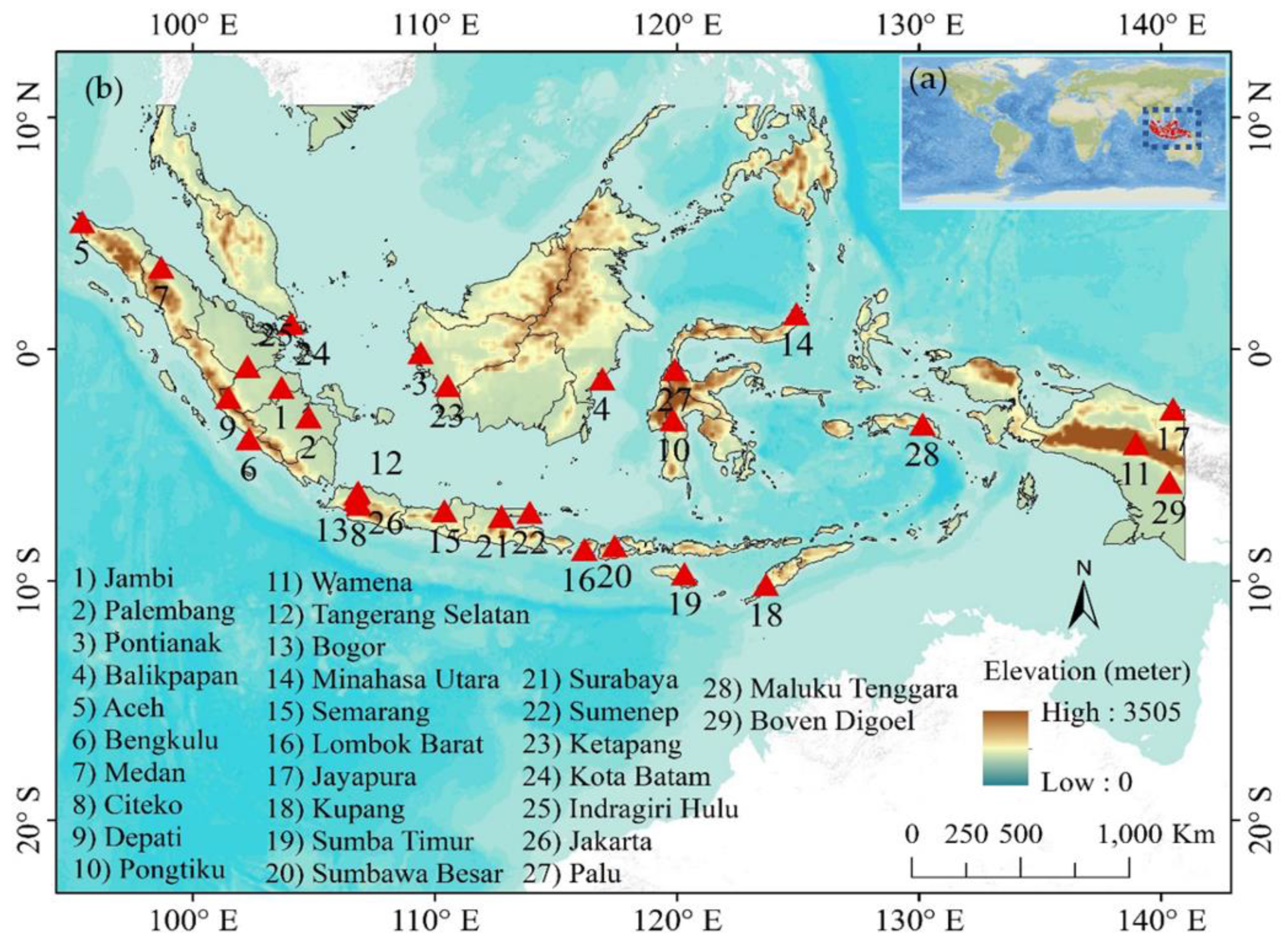
2. Study Area
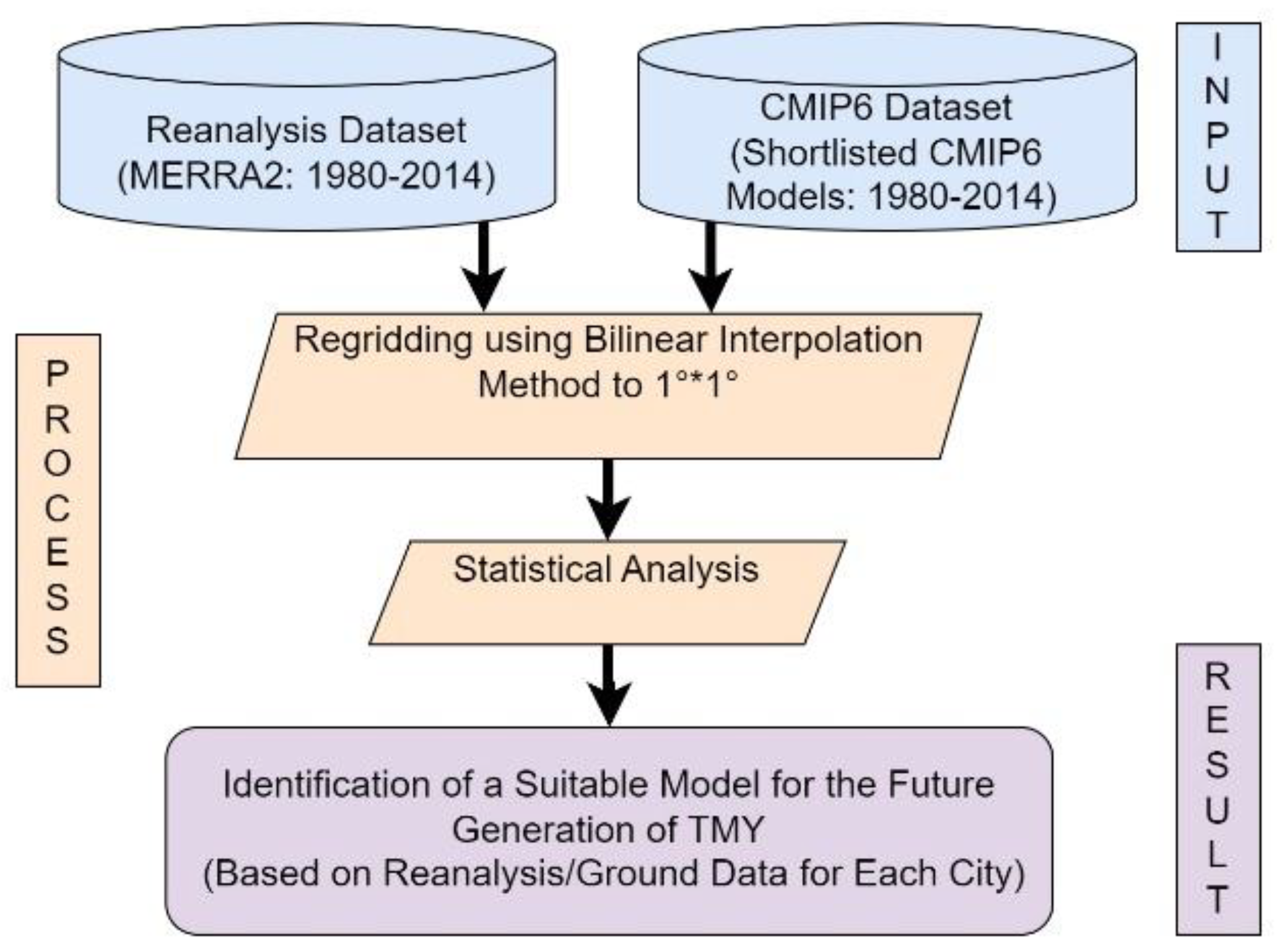
3. Data and Method
3.1. Selection of CMIP6 GCMs
3.2. Reanalysis Dataset
3.3. The Measure of the Statistical Performance
3.4. Ranking of the GCM
4. Results and Discussion
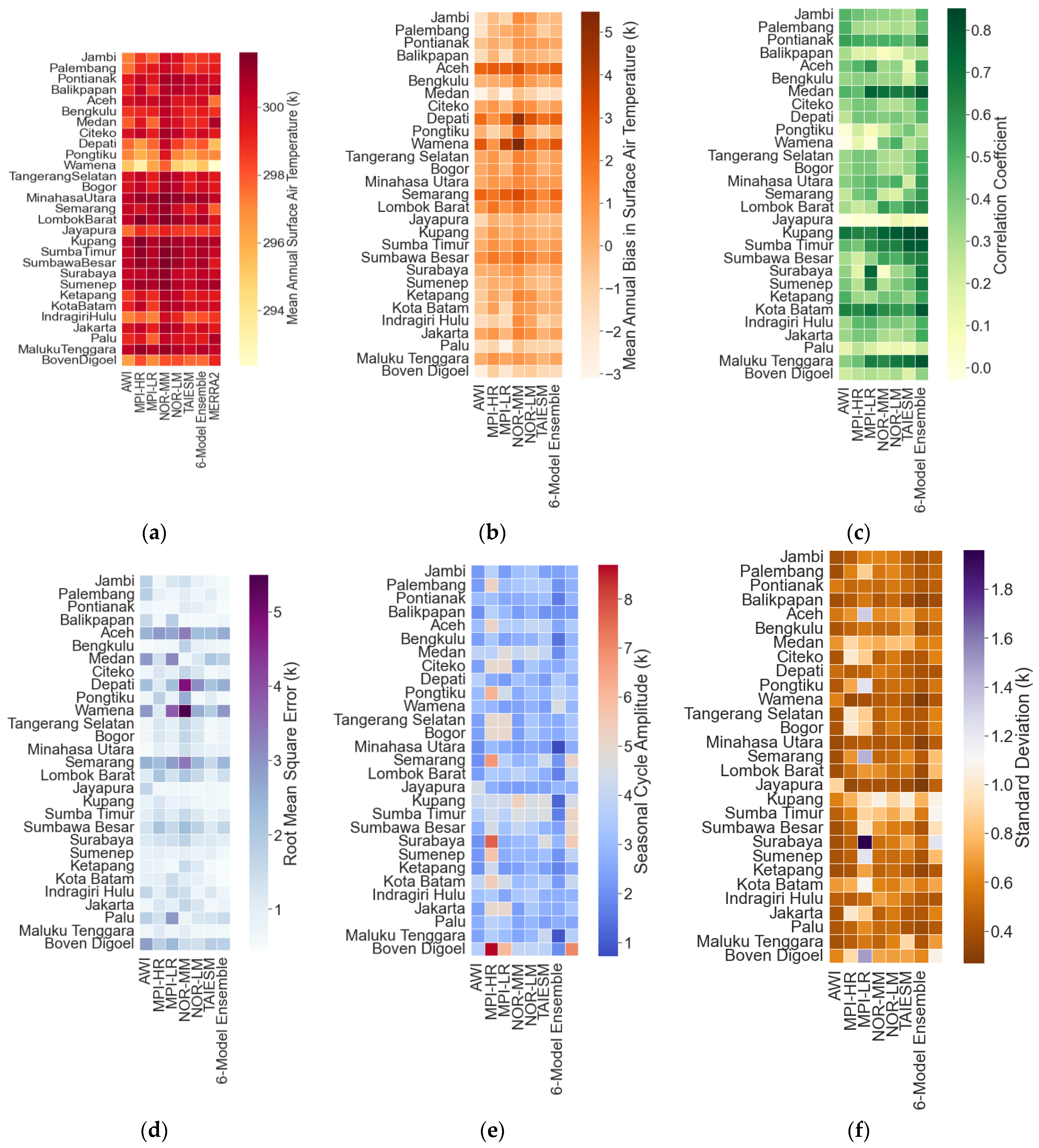
4.1. Surface Air Temperature
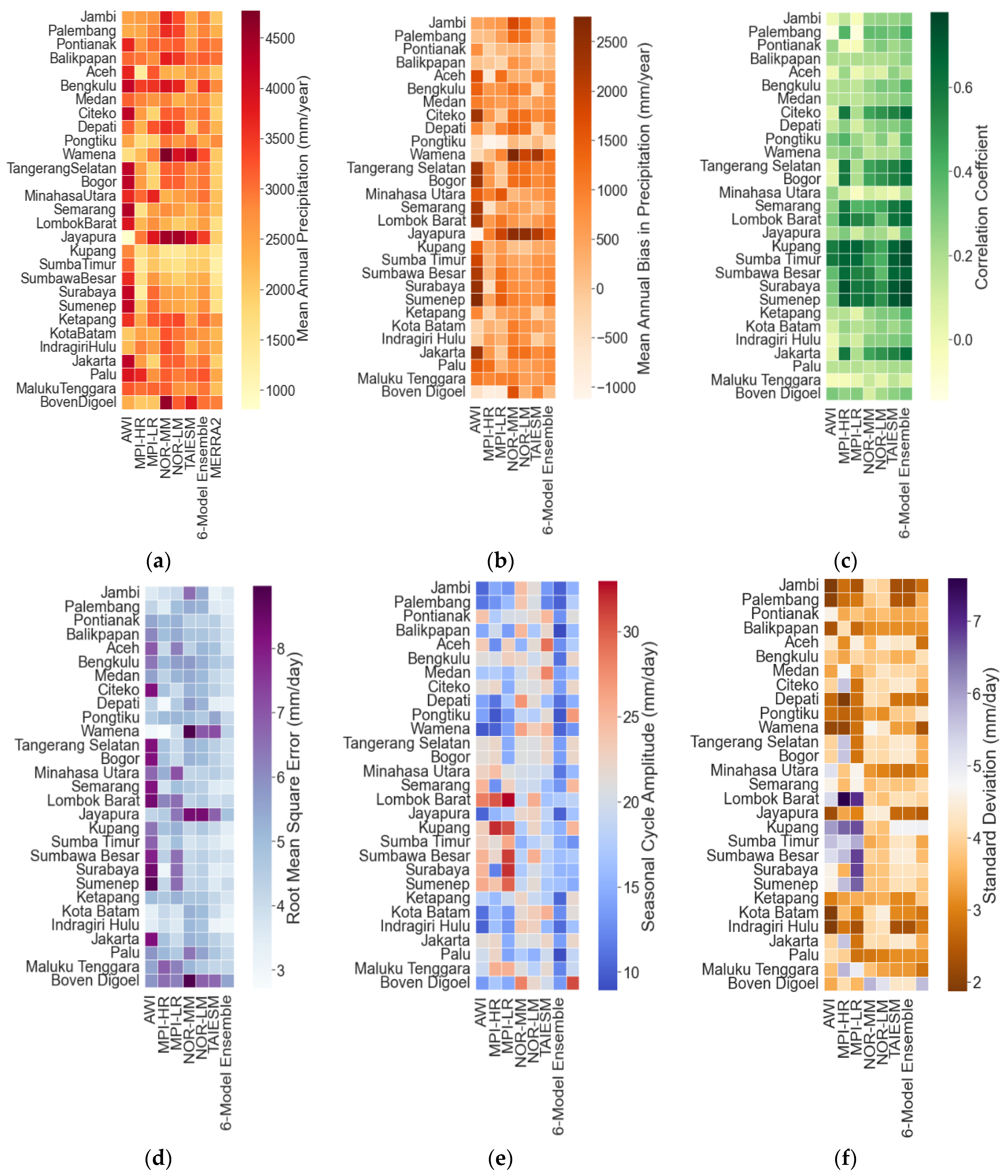
4.2. Precipitation
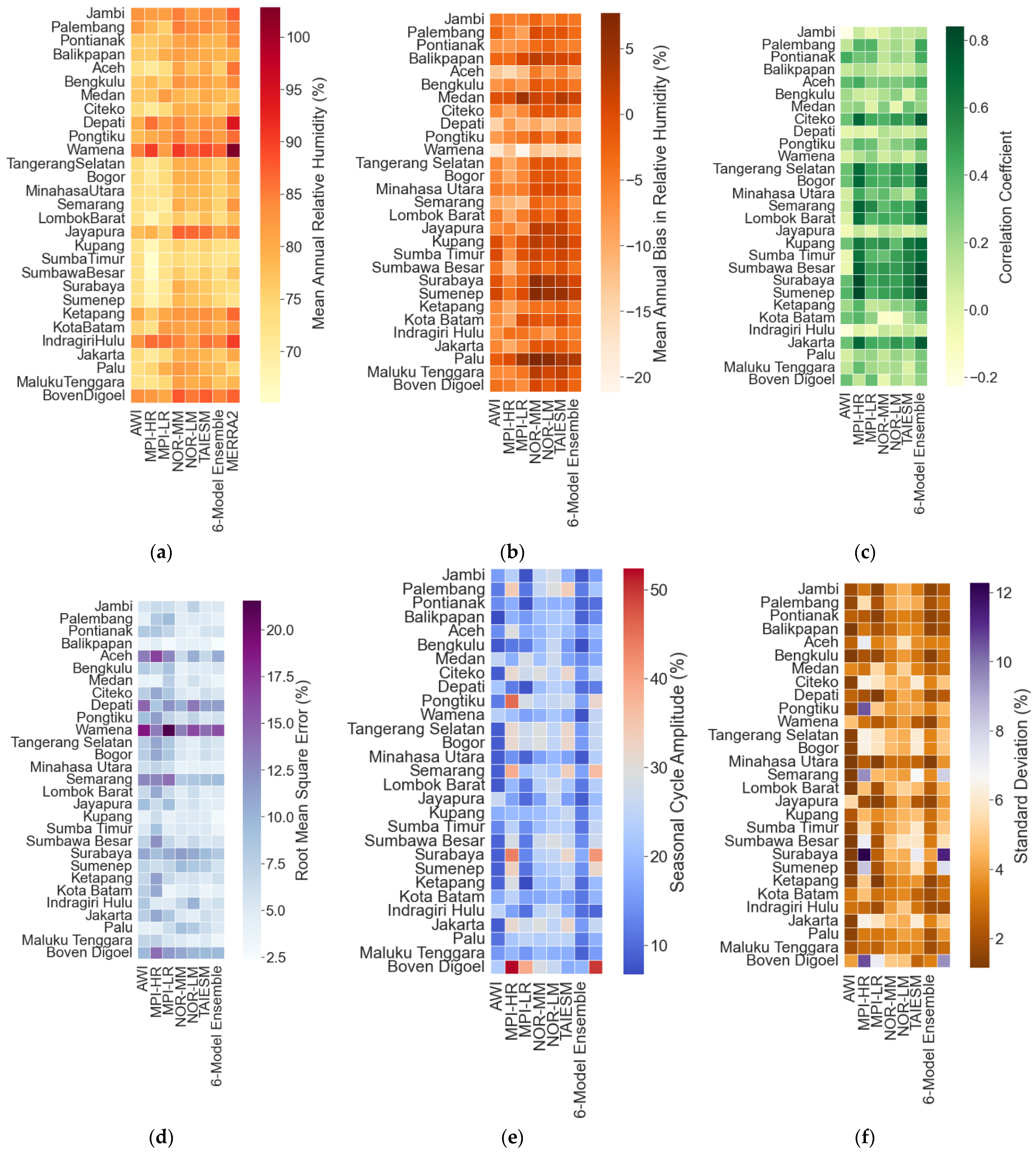
4.3. Relative Humidity
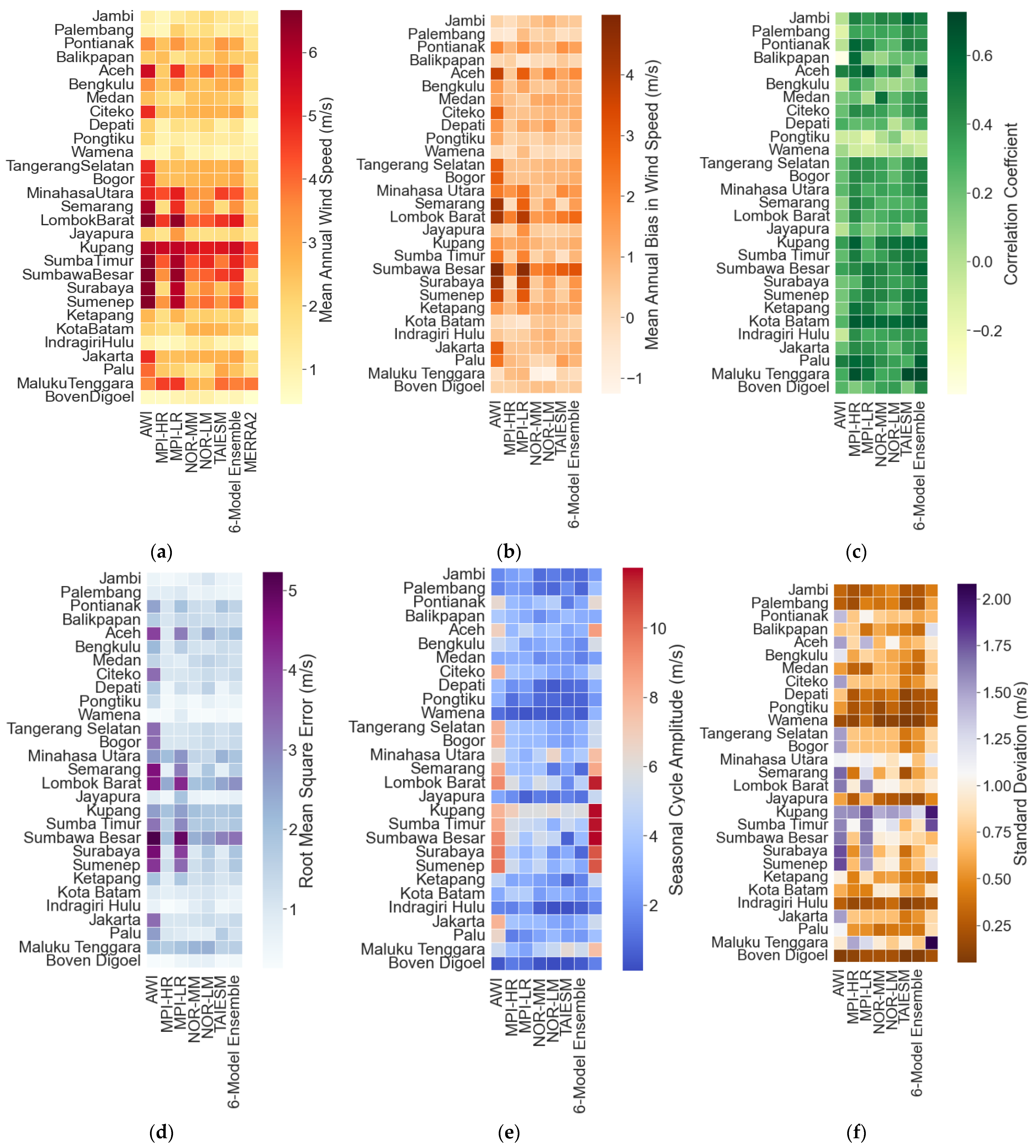
4.4. Wind Speed
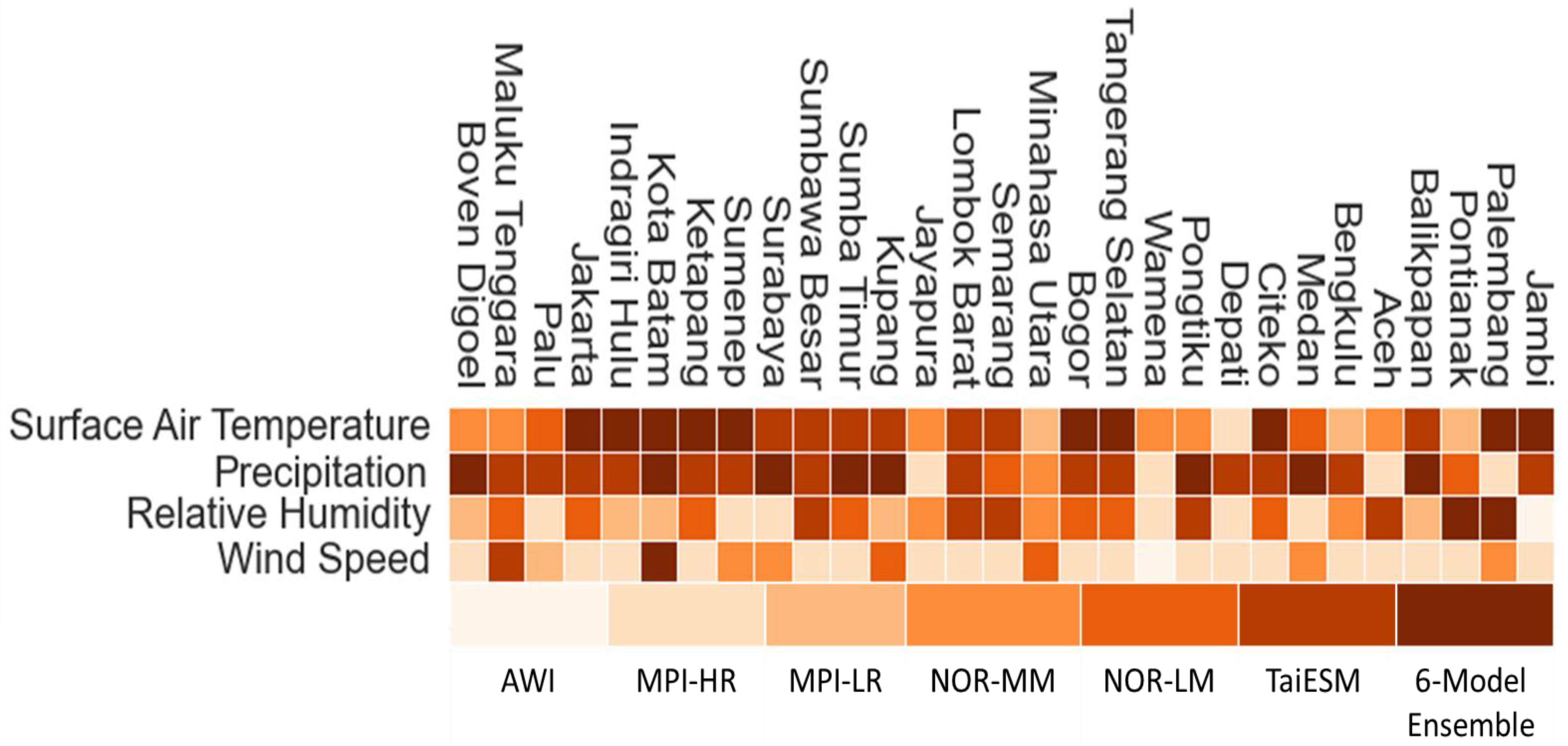
4.5. Ranking of the GCMs
5. Conclusions
- (i)
- From 1980–2014, the mean annual surface air temperature varies from 290 K to 302 K for all the cities. The MBE calculated for mean annual surface temperature derived from 6 GCMs and 6-Model Ensemble ranges from −3 to 5 K. In the case of the 6-Model Ensemble, out of 29 cities, 20 (9) cities showed warm (cold) biases. The performance of each GCM alters concerning the city. Among all the GCMs, including 6-Model Ensemble, TaiESM performed best in 14 cities, followed by the 6-Model Ensemble, which performed well over 10 cities. For Indonesian cities, AWI was the worst performing GCM which was not found to be suitable over any of the cities. Except for a few cities, the performance of each GCM in terms of standard deviation and RMSE is very similar. For most cities, the difference between the seasonal amplitude calculated by each GCM, including 6-Model Ensemble, is less than 0.5 K. While in some cities like Jayapura and Sumbawa, this difference has been observed up to 1.5 K.
- (ii)
- Regarding precipitation, corresponding to mean annual precipitation, 6-Model Ensemble shows the cold biases across all the cities (except Pongtiku). These cold biases range from 96.4 to 1513.39 mm/year. Among all GCMs, for precipitation, the performance of TaiESM was outstanding in 14 cities.
- (iii)
- Compared to reference data for most cities, the mean annual relative humidity derived from all the GCMs indicates negative biases. In the case of relative humidity, the performance of NOR-LM was better over seven cities.
- (iv)
- Compared to reference data, very minimal divergence has been noted in the GCM/6-Model Ensemble derived for mean annual wind speed. For wind speed, MPI-HR performed outstandingly in 19 cities.
Author Contributions
Funding
Institutional Review Board Statement
Informed Consent Statement
Data Availability Statement
Acknowledgments
Conflicts of Interest
Appendix A

| Cities | Surface Air Temperature | Precipitation | Relative Humidity | Wind Speed |
|---|---|---|---|---|
| Jambi | 6-Model Ensemble | TaiESM | AWI | MPI-HR |
| Palembang | 6-Model Ensemble | MPI-HR | 6-Model Ensemble | NOR-MM |
| Pontianak | MPI-LR | NOR-LM | 6-Model Ensemble | MPI-HR |
| Balikpapan | TAIESM | 6-Model Ensemble | MPI-LR | MPI-HR |
| Aceh | NOR-MM | MPI-HR | TaiESM | MPI-HR |
| Bengkulu | MPI-LR | TaiESM | NOR-MM | MPI-HR |
| Medan | NOR-LM | 6-Model Ensemble | MPI-HR | NOR-MM |
| Citeko | 6-Model Ensemble | TaiESM | NOR-LM | MPI-HR |
| Depati | MPI-HR | TaiESM | MPI-HR | MPI-HR |
| Pongtiku | NOR-MM | 6-Model Ensemble | TaiESM | MPI-HR |
| Wamena | NOR-MM | MPI-HR | MPI-HR | AWI |
| Tangerang Selatan | 6-Model Ensemble | TaiESM | NOR-LM | MPI-HR |
| Bogor | 6-Model Ensemble | TaiESM | NOR-LM | MPI-HR |
| Minahasa Utara | MPI-LR | NOR-MM | NOR-MM | NOR-LM |
| Semarang | TaiESM | NOR-LM | TaiESM | MPI-HR |
| Lombok Barat | TaiESM | TaiESM | TaiESM | MPI-HR |
| Jayapura | NOR-MM | MPI-HR | NOR-MM | MPI-HR |
| Kupang | TaiESM | 6-Model Ensemble | MPI-LR | NOR-LM |
| Sumba Timur | TaiESM | 6-Model Ensemble | NOR-LM | MPI-HR |
| Sumbawa Besar | TaiESM | TaiESM | TaiESM | MPI-HR |
| Surabaya | TaiESM | 6-Model Ensemble | MPI-HR | NOR-MM |
| Sumenep | 6-Model Ensemble | TaiESM | MPI-HR | NOR-MM |
| Ketapang | 6-Model Ensemble | TaiESM | NOR-LM | MPI-HR |
| Kota Batam | 6-Model Ensemble | 6-Model Ensemble | MPI-LR | 6-Model Ensemble |
| Indragiri Hulu | 6-Model Ensemble | TaiESM | MPI-LR | MPI-HR |
| Jakarta | 6-Model Ensemble | TaiESM | NOR-LM | MPI-HR |
| Palu | NOR-LM | TaiESM | MPI-HR | MPI-LR |
| Maluku Tenggara | NOR-MM | TaiESM | NOR-LM | TaiESM |
| Boven Digoel | NOR-MM | 6-Model Ensemble | MPI-LR | MPI-HR |
References
- Upadhyay, R.K. Markers for global climate change and its impact on social, biological and ecological systems: A review. Am. J. Clim. Chang. 2020, 9, 159. [Google Scholar] [CrossRef]
- Allan, R.P.; Hawkins, E.; Bellouin, N.; Collins, B. IPCC, 2021: Summary for Policymakers; IPCC: Cambridge, UK, 2021. [Google Scholar]
- Latha, R.; Murthy, B.S.; Vinayak, B. Aerosol-induced perturbation of surface fluxes over different landscapes in a tropical region. Int. J. Remote Sens. 2019, 40, 8203–8221. [Google Scholar] [CrossRef]
- Bhanage, V.; Kulkarni, S.; Sharma, R.; Lee, H.S.; Gedam, S. Enumerating and Modelling the Seasonal alterations of Surface Urban Heat and Cool Island: A Case Study over Indian Cities. Urban Sci. 2023, 7, 38. [Google Scholar] [CrossRef]
- Vinayak, B.; Lee, H.S.; Gedam, S.; Latha, R. Impacts of future urbanization on urban microclimate and thermal comfort over the Mumbai metropolitan region, India. Sustain. Cities Soc. 2022, 79, 103703. [Google Scholar] [CrossRef]
- Kulkarni, S.S.; Wardlow, B.D.; Bayissa, Y.A.; Tadesse, T.; Svoboda, M.D.; Gedam, S.S. Developing a remote sensing-based combined drought indicator approach for agricultural drought monitoring over Marathwada, India. Remote Sens. 2020, 12, 2091. [Google Scholar] [CrossRef]
- Latha, R.; Vinayak, B.; Murthy, B.S. Response of heterogeneous vegetation to aerosol radiative forcing over a northeast Indian station. J. Environ. Manag. 2018, 206, 1224–1232. [Google Scholar] [CrossRef]
- Gusain, A.; Ghosh, S.; Karmakar, S. Added value of CMIP6 over CMIP5 models in simulating Indian summer monsoon rainfall. Atmos. Res. 2020, 232, 104680. [Google Scholar] [CrossRef]
- Taye, M.T.; Ntegeka, V.; Ogiramoi, N.P.; Willems, P. Assessment of climate change impact on hydrological extremes in two source regions of the Nile River Basin. Hydrol. Earth Syst. Sci. 2011, 15, 209–222. [Google Scholar] [CrossRef]
- Kamworapan, S.; Bich Thao, P.T.; Gheewala, S.H.; Pimonsree, S.; Prueksakorn, K. Evaluation of CMIP6 GCMs for simulations of temperature over Thailand and nearby areas in the early 21st century. Heliyon 2021, 7, e08263. [Google Scholar] [CrossRef]
- Kamruzzaman, M.; Shahid, S.; Islam, A.R.M.; Hwang, S.; Cho, J.; Zaman, M.; Uz, A.; Ahmed, M.; Rahman, M.; Hossain, M. Comparison of CMIP6 and CMIP5 model performance in simulating historical precipitation and temperature in Bangladesh: A preliminary study. Theor. Appl. Climatol. 2021, 145, 1385–1406. [Google Scholar] [CrossRef]
- Ândrea, M.; Firpo, F.; Guimarães, S.; Dantas, L.G.; Guatura, M.; Alves, L.M.; Chadwick, R. Assessment of CMIP models’ performance in simulating present-day climate in Brazil. Front. Clim. 2022, 4, 170. [Google Scholar] [CrossRef]
- Seker, M.; Gumus, V. Projection of temperature and precipitation in the Mediterranean region through multi-model ensemble from CMIP6. Atmos. Res. 2022, 280, 106440. [Google Scholar] [CrossRef]
- Lu, K.; Arshad, M.; Ma, X.; Ullah, I.; Wang, J.; Shao, W. Evaluating observed and future spatiotemporal changes in precipitation and temperature across China based on CMIP6-GCMs. Int. J. Climatol. 2022, 42, 7703–7729. [Google Scholar] [CrossRef]
- Zhu, Y.-Y.; Yang, S. Evaluation of CMIP6 for historical temperature and precipitation over the Tibetan Plateau and its comparison with CMIP5. Adv. Clim. Chang. Res. 2020, 11, 239–251. [Google Scholar] [CrossRef]
- Shiru, M.S.; Chung, E.-S. Performance evaluation of CMIP6 global climate models for selecting models for climate projection over Nigeria. Theor. Appl. Climatol. 2021, 146, 599–615. [Google Scholar] [CrossRef]
- Srivastava, A.; Grotjahn, R.; Ullrich, P.A. Evaluation of historical CMIP6 model simulations of extreme precipitation over contiguous US regions. Weather Clim. Extrem. 2020, 29, 100268. [Google Scholar] [CrossRef]
- Ge, F.; Zhu, S.; Luo, H.; Zhi, X.; Wang, H. Future changes in precipitation extremes over Southeast Asia: Insights from CMIP6 multi-model ensemble. Environ. Res. Lett. 2021, 16, 24013. [Google Scholar] [CrossRef]
- Mamalakis, A. Links of Climate Variability and Change with Regional Hydroclimate: Predictability, Trends, and Physical Mechanisms on Seasonal to Decadal Scales; University of California: Irvine, CA, USA, 2020; ISBN 9798557021494. [Google Scholar]
- Oke, T.R.; Mills, G.; Christen, A.; Voogt, J.A. Urban Climates; Cambridge University Press: Cambridge, UK, 2017; ISBN 0521849500. [Google Scholar]
- Videras Rodríguez, M.; Sánchez Cordero, A.; Gómez Melgar, S.; Andújar Márquez, J.M. Impact of global warming in subtropical climate buildings: Future trends and mitigation strategies. Energies 2020, 13, 6188. [Google Scholar] [CrossRef]
- Vinayak, B.; Lee, H.S.; Gedem, S. Prediction of Land Use and Land Cover Changes in Mumbai City, India, Using Remote Sensing Data and a Multilayer Perceptron Neural Network-Based Markov Chain Model. Sustainability 2021, 13, 471. [Google Scholar] [CrossRef]
- Atiqi, R.; Dimyati, M.; Gamal, A.; Pramayuda, R. Appraisal of Building Price in Urban Area Using Light Detection and Ranging (LiDAR) Data in Depok City. Land 2022, 11, 1320. [Google Scholar] [CrossRef]
- Gao, M.; Wang, Z.; Yang, H. Review of Urban Flood Resilience: Insights from Scientometric and Systematic Analysis. Int. J. Environ. Res. Public Health 2022, 19, 8837. [Google Scholar] [CrossRef] [PubMed]
- Saputra, M.H.; Lee, H.S. Prediction of land use and land cover changes for North Sumatra, Indonesia, using an artificial-neural-network-based cellular automaton. Sustainability 2019, 11, 3024. [Google Scholar] [CrossRef]
- Hamed, M.M.; Nashwan, M.S.; Shiru, M.S.; Shahid, S. Comparison between CMIP5 and CMIP6 Models over MENA Region Using Historical Simulations and Future Projections. Sustainability 2022, 14, 10375. [Google Scholar] [CrossRef]
- Lun, Y.; Liu, L.; Cheng, L.; Li, X.; Li, H.; Xu, Z. Assessment of GCMs simulation performance for precipitation and temperature from CMIP5 to CMIP6 over the Tibetan Plateau. Int. J. Climatol. 2021, 41, 3994–4018. [Google Scholar] [CrossRef]
- Touzé-Peiffer, L.; Barberousse, A.; Le Treut, H. The Coupled Model Intercomparison Project: History, uses, and structural effects on climate research. Wiley Interdiscip. Rev. Clim. Chang. 2020, 11, e648. [Google Scholar] [CrossRef]
- Bosilovich, M.G. MERRA-2: Initial Evaluation of the Climate; National Aeronautics and Space Administration, Goddard Space Flight Center: Greenbelt, MD, USA, 2015.
- Rohmat, F.I.W.; Stamataki, I.; Sa’adi, Z.; Fitriani, D. Flood analysis using HEC-RAS: The case study of Majalaya, Indonesia under the CMIP6 projection. In Proceedings of the EGU General Assembly Conference, Vienna, Austria, 23–27 May 2022. [Google Scholar] [CrossRef]
- Sa’adi, Z.; Rohmat, F.I.W.; Stamataki, I.; Shahid, S.; Iqbal, Z.; Yaseen, Z.M.; Yusop, Z.; Alias, N.E. Spatiotemporal Rainfall Projection in Majalaya basin, West Java, Indonesia under CMIP6 Scenarios. Res. Sq. 2022. [Google Scholar] [CrossRef]
- Kurniadi, A.; Weller, E.; Kim, Y.-H.; Min, S.-K. Evaluation of Coupled Model Intercomparison Project Phase 6 model-simulated extreme precipitation over Indonesia. Int. J. Climatol. 2023, 43, 174–196. [Google Scholar] [CrossRef]
- Desmet, Q.; Ngo-Duc, T. A novel method for ranking CMIP6 global climate models over the southeast Asian region. Int. J. Climatol. 2022, 42, 97–117. [Google Scholar] [CrossRef]
- Pimonsree, S.; Kamworapan, S.; Gheewala, S.H.; Thongbhakdi, A.; Prueksakorn, K. Evaluation of CMIP6 GCMs performance to simulate precipitation over Southeast Asia. Atmos. Res. 2023, 282, 106522. [Google Scholar] [CrossRef]


| No | GCM ID | Acronym | Spatial Resolution | Period | Institution |
|---|---|---|---|---|---|
| 1 | NorESM2-MM | NOR-MM | 1° × 1° | Jan. 1980–Dec. 2014 | Norwegian-Climate Centre/Norway |
| 2 | NorESM2-LM | NOR-LM | 2.5° × 2.5° | Jan. 1980–Dec. 2014 | Norwegian-Climate Centre/Norway |
| 3 | MPIESM 1-2-HR | MPI-HR | 1° × 1° | Jan. 1980–Dec. 2014 | Max Planck Institute of Meteorology/Germany |
| 4 | MPI-ESM 1-2-LR | MPI-LR | 2.5° × 2.5° | Jan. 1980–Dec. 2014 | Max Planck Institute of Meteorology/Germany |
| 5 | RCEC. TaiESM1 | TaiESM | 1° × 1° | Jan. 1980–Dec. 2014 | Research Centre for Environmental Changes/Taiwan, China |
| 6. | AWI-CM-1-1-MR | AWI | 1° × 1° | Jan. 1980–Dec. 2014 | The Alfred Wegener Institute/ Germany |
| Statistical Measure | Formula |
|---|---|
| Correlation Coefficient | |
| Standard Deviation | |
| Mean Annual | |
| Mean Bias Error | |
| Mean Seasonal Cycle Amplitude | |
| Root Mean Square Error |
Disclaimer/Publisher’s Note: The statements, opinions and data contained in all publications are solely those of the individual author(s) and contributor(s) and not of MDPI and/or the editor(s). MDPI and/or the editor(s) disclaim responsibility for any injury to people or property resulting from any ideas, methods, instructions or products referred to in the content. |
© 2023 by the authors. Licensee MDPI, Basel, Switzerland. This article is an open access article distributed under the terms and conditions of the Creative Commons Attribution (CC BY) license (https://creativecommons.org/licenses/by/4.0/).
Share and Cite
Bhanage, V.; Lee, H.S.; Kubota, T.; Pradana, R.P.; Fajary, F.R.; Arya Putra, I.D.G.; Nimiya, H. City-Wise Assessment of Suitable CMIP6 GCM in Simulating Different Urban Meteorological Variables over Major Cities in Indonesia. Climate 2023, 11, 100. https://doi.org/10.3390/cli11050100
Bhanage V, Lee HS, Kubota T, Pradana RP, Fajary FR, Arya Putra IDG, Nimiya H. City-Wise Assessment of Suitable CMIP6 GCM in Simulating Different Urban Meteorological Variables over Major Cities in Indonesia. Climate. 2023; 11(5):100. https://doi.org/10.3390/cli11050100
Chicago/Turabian StyleBhanage, Vinayak, Han Soo Lee, Tetsu Kubota, Radyan Putra Pradana, Faiz Rohman Fajary, I Dewa Gede Arya Putra, and Hideyo Nimiya. 2023. "City-Wise Assessment of Suitable CMIP6 GCM in Simulating Different Urban Meteorological Variables over Major Cities in Indonesia" Climate 11, no. 5: 100. https://doi.org/10.3390/cli11050100