
Overview of the Spectral Coherence between Planetary Resonances and Solar and Climate Oscillations


Abstract
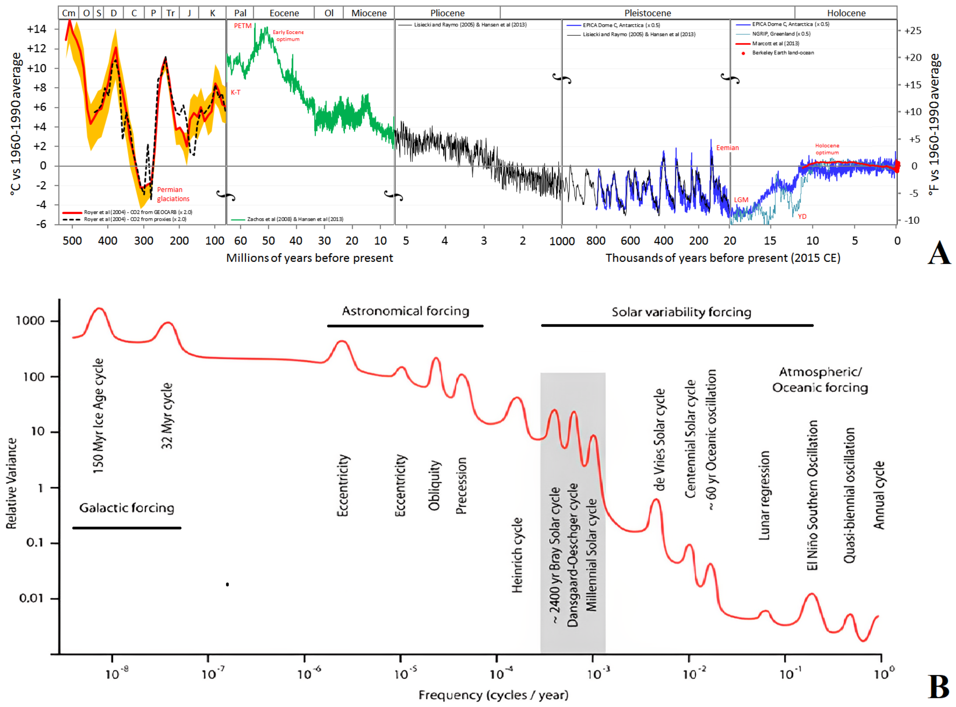
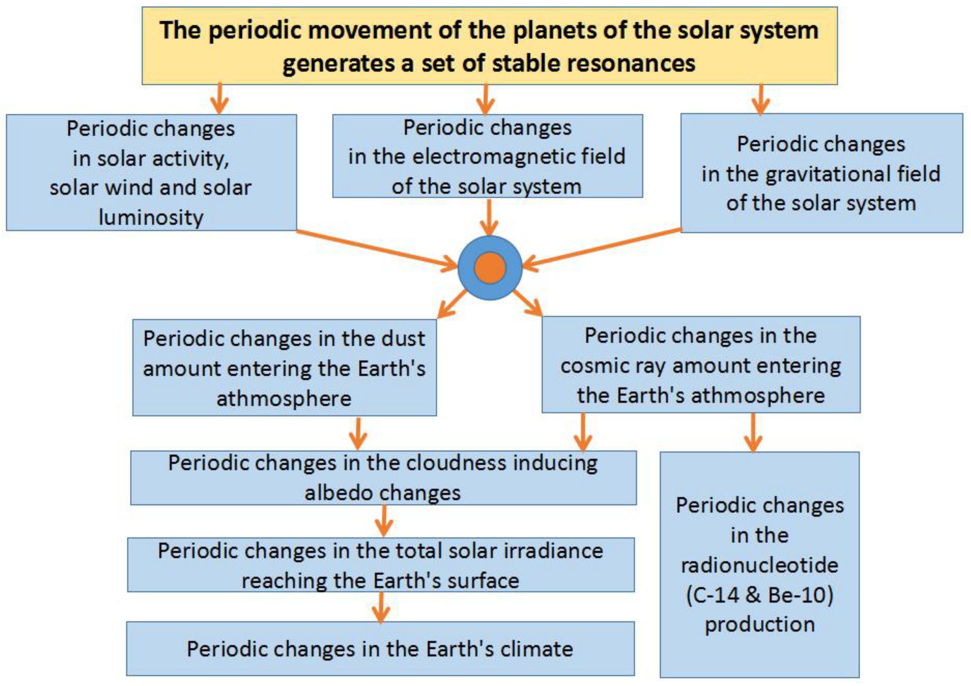
:1. Introduction
2. Overview of the Planetary Hypothesis of the Origin of Solar Activity Cycles
3. Empirical Evidences for the Planetary Origin of Solar and Climate Variability Cycles
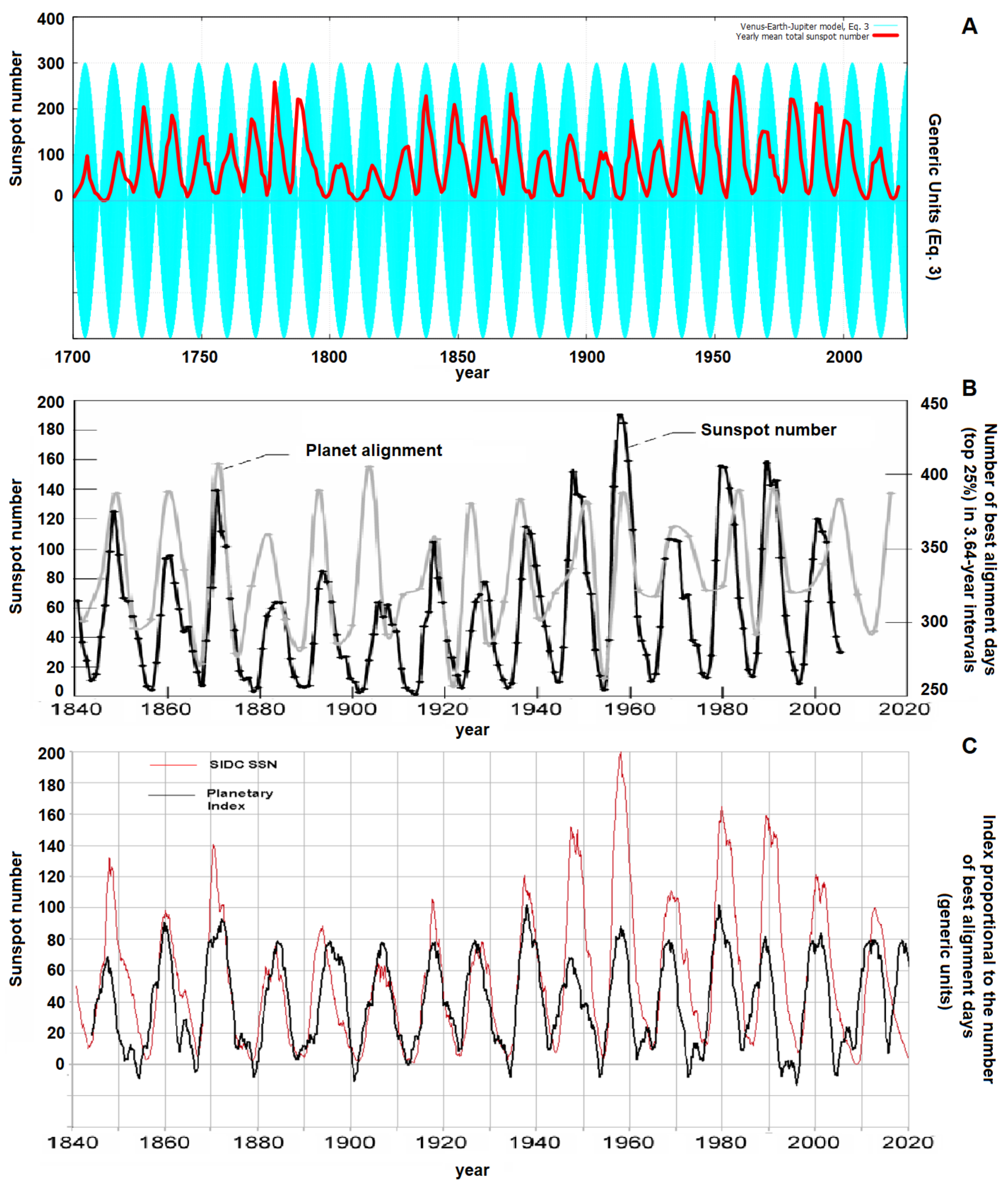
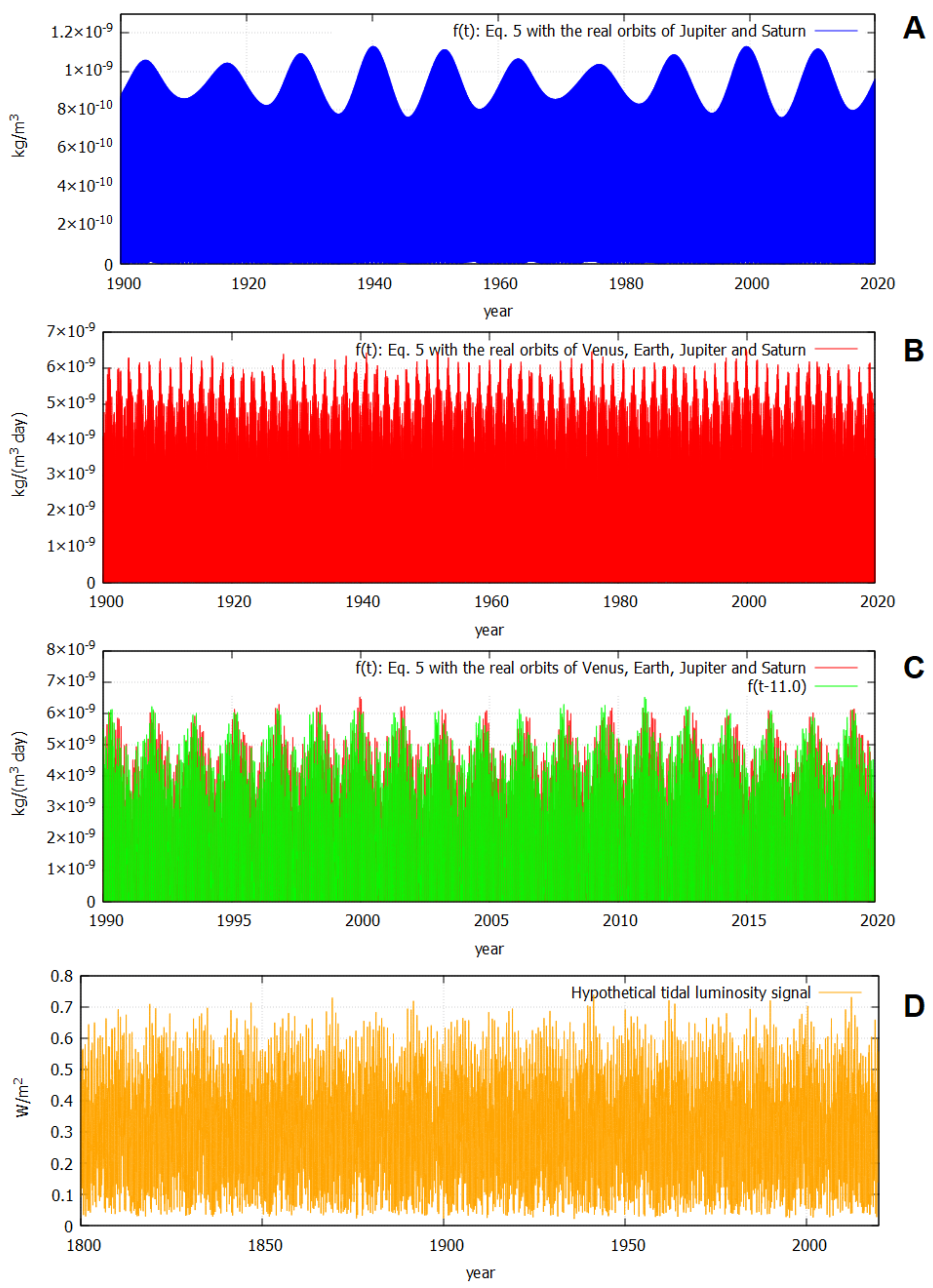
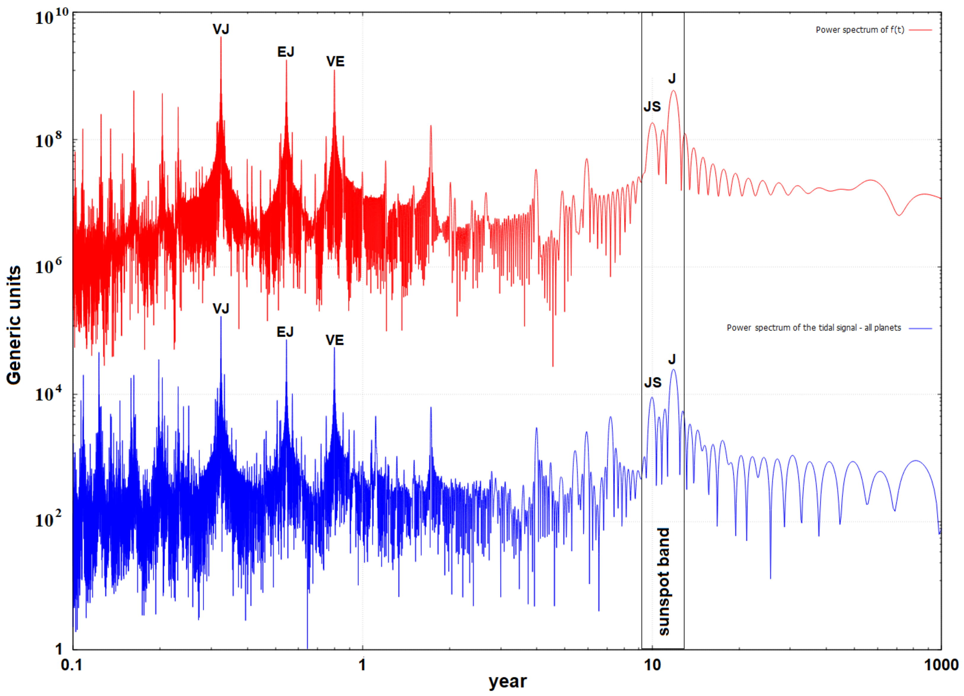
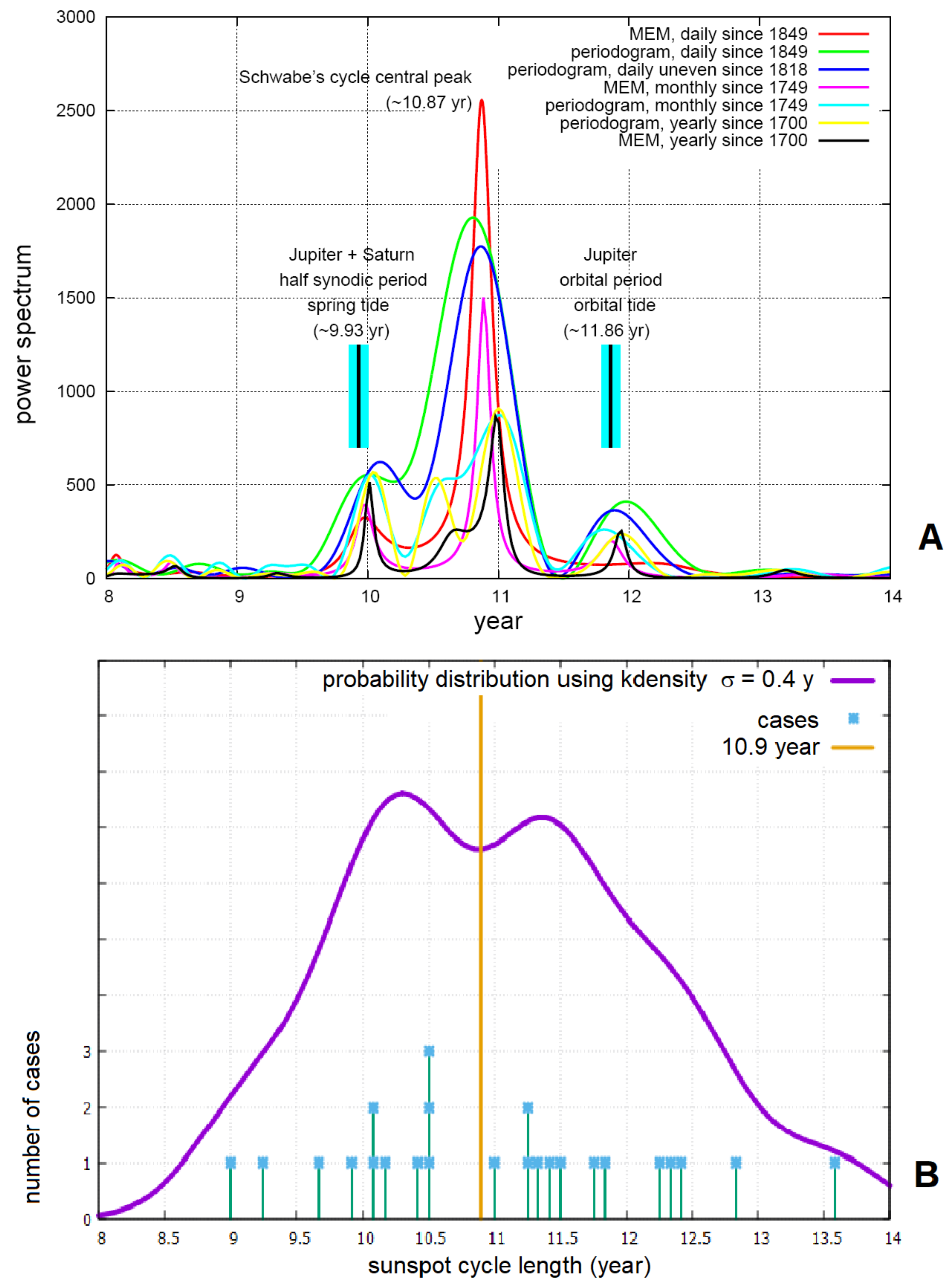
3.1. The Venus–Earth–Jupiter–Saturn Model for the Schwabe 11-Year Solar-Activity Cycle
3.2. Empirical Evidences for Planetary Control of Solar Variability across Several Timescales
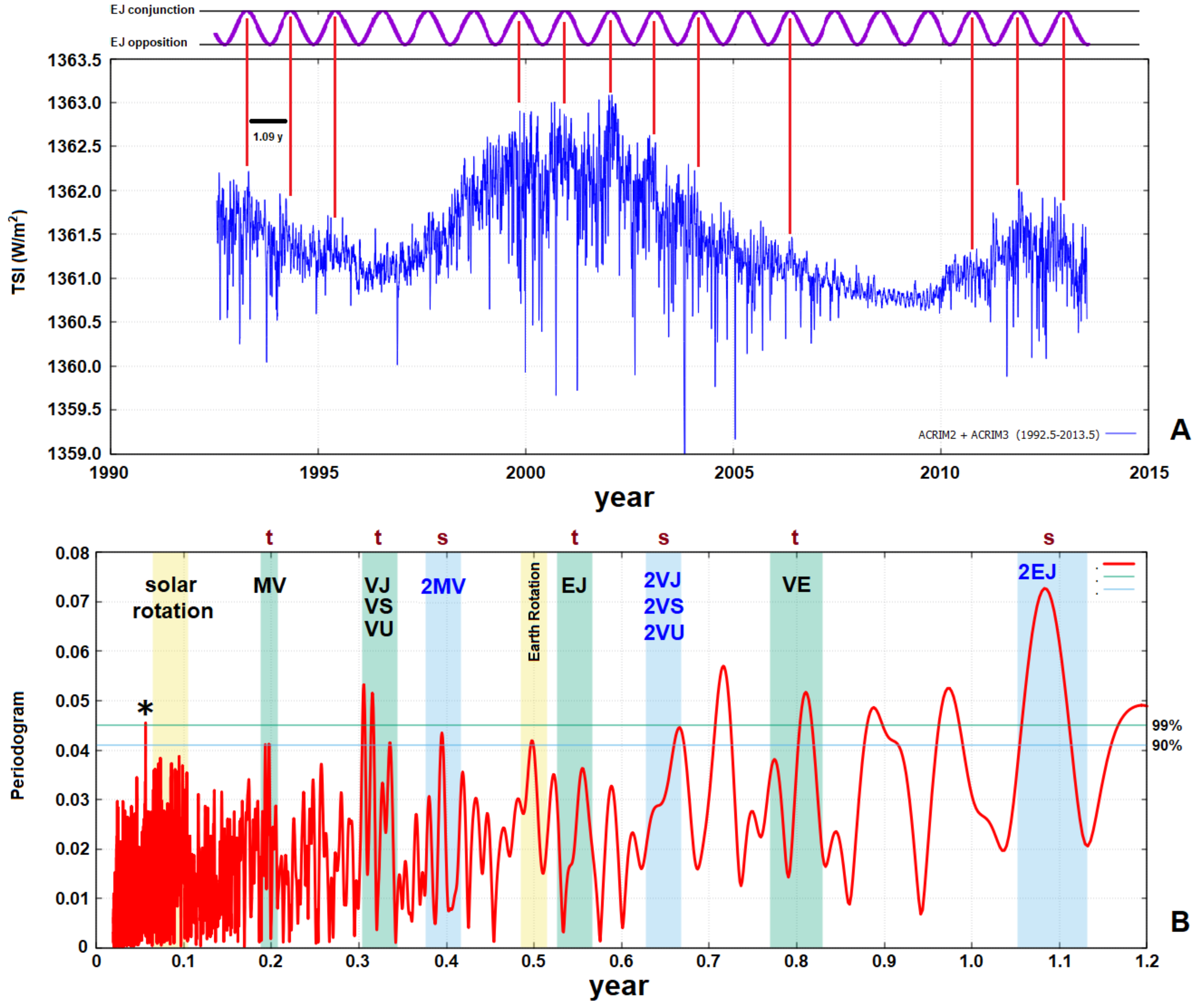
3.2.1. Monthly to Annual Timescales
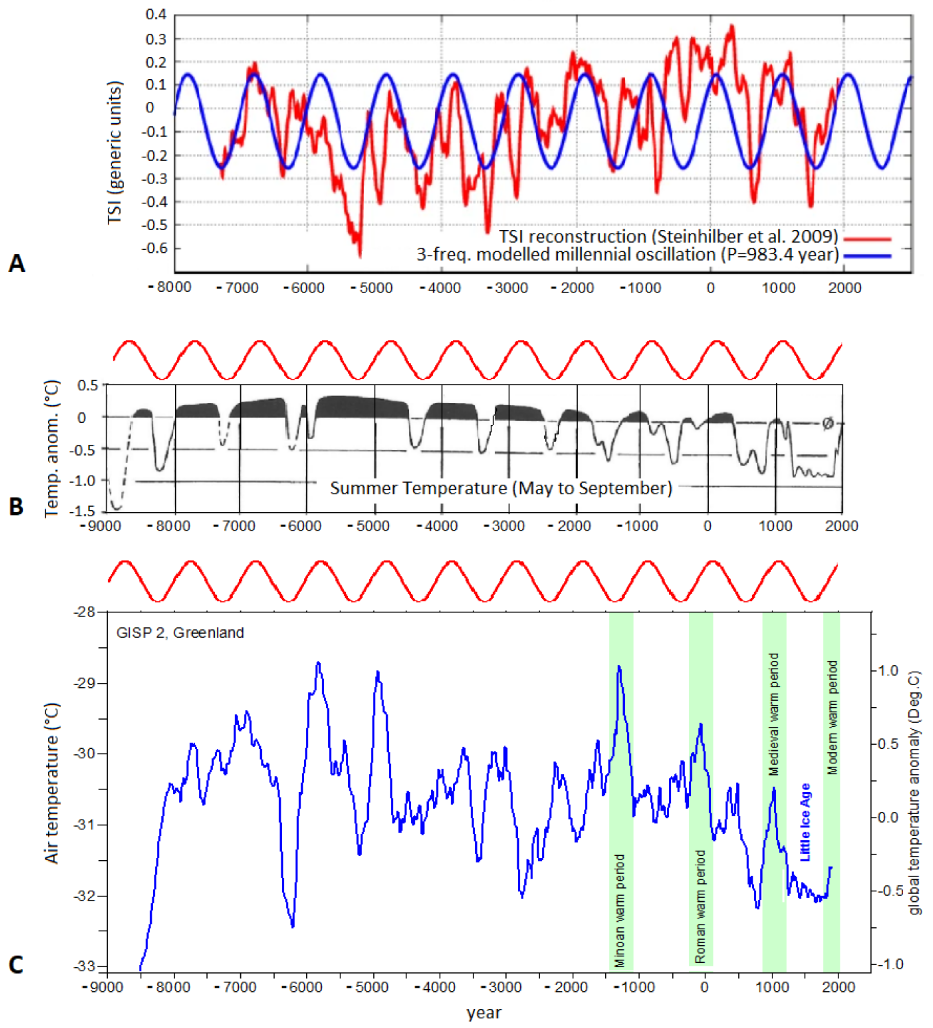
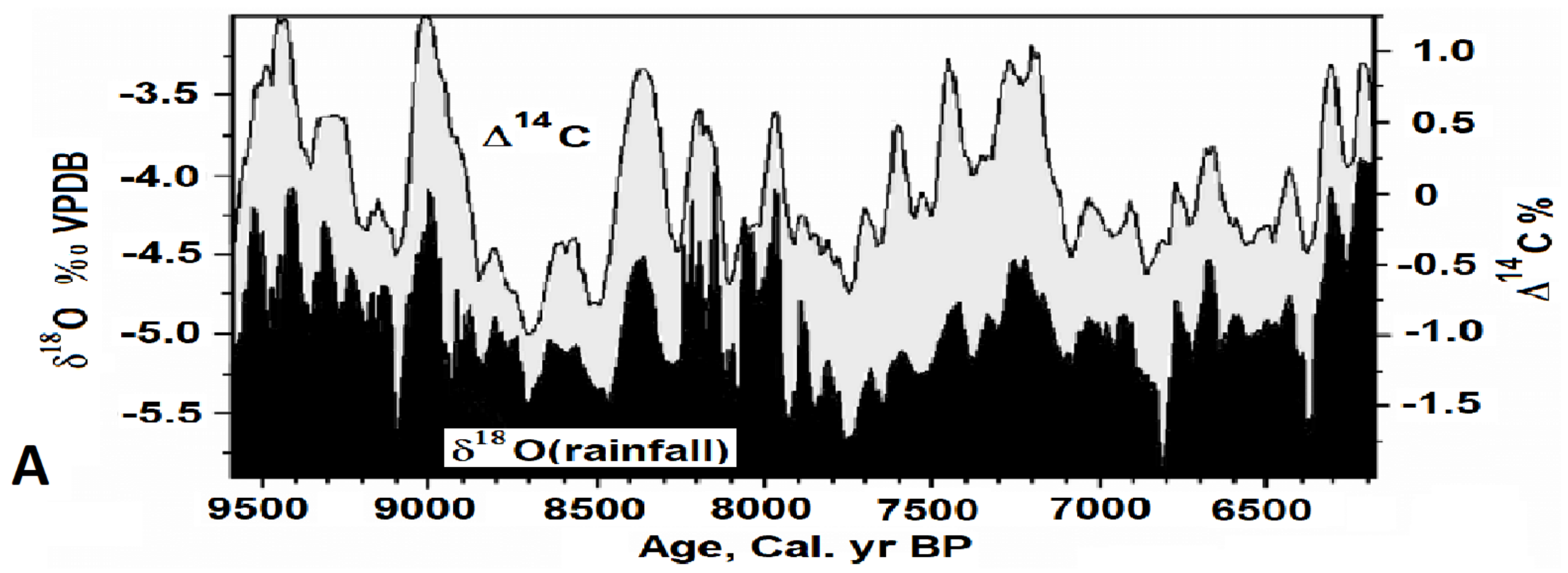
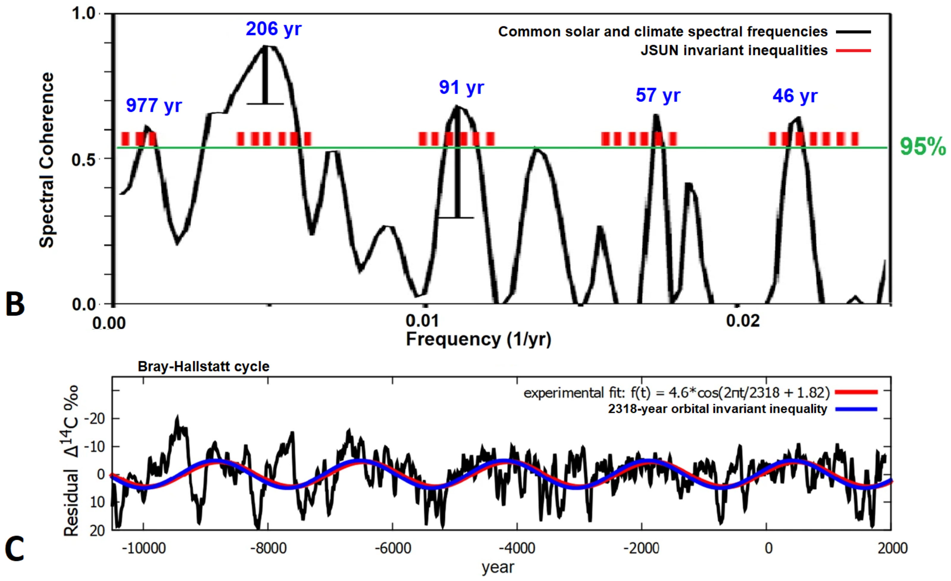
3.2.2. Multidecadal to Millennial Timescales
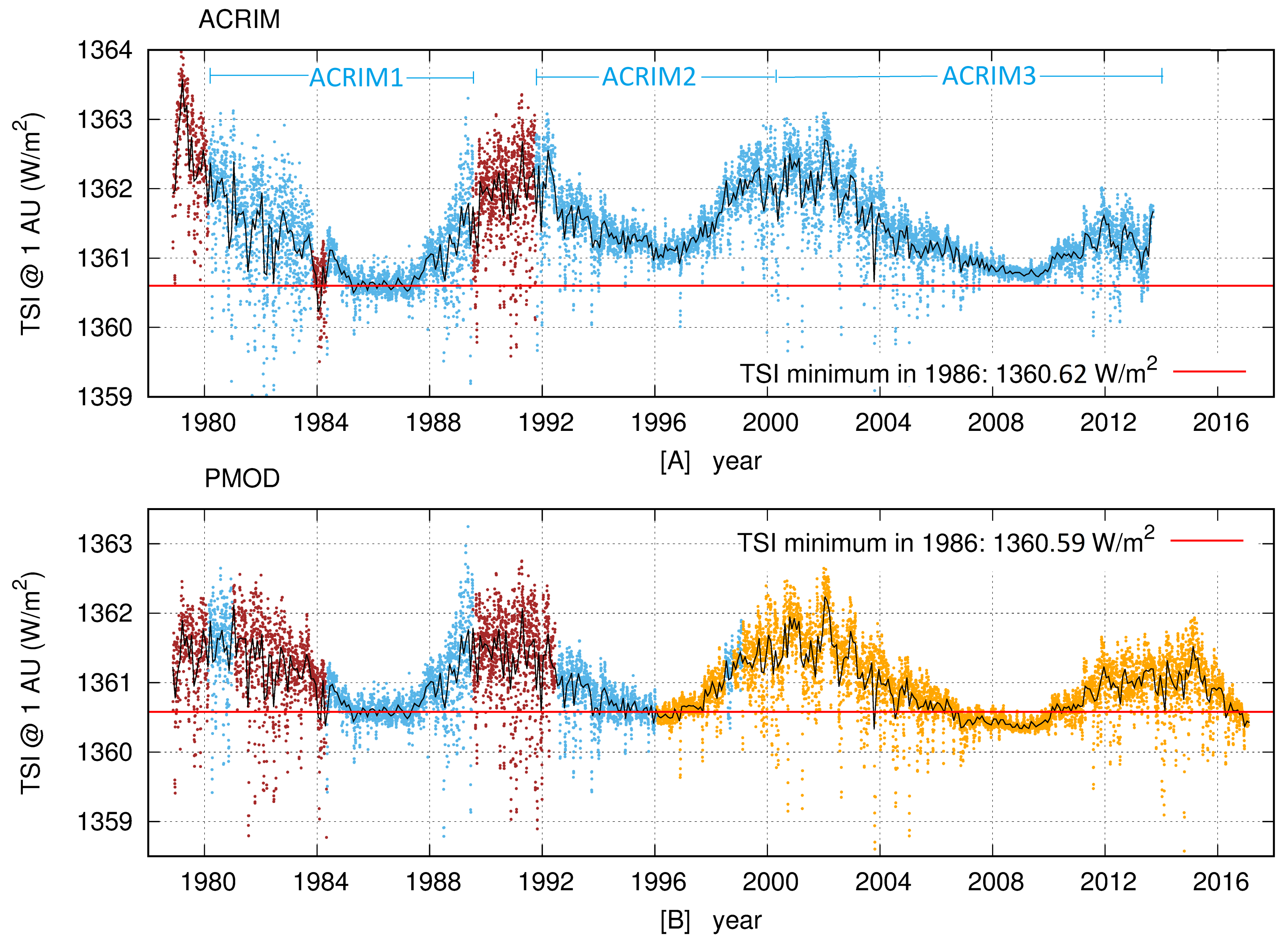
3.2.3. Miscellaneous Evidences
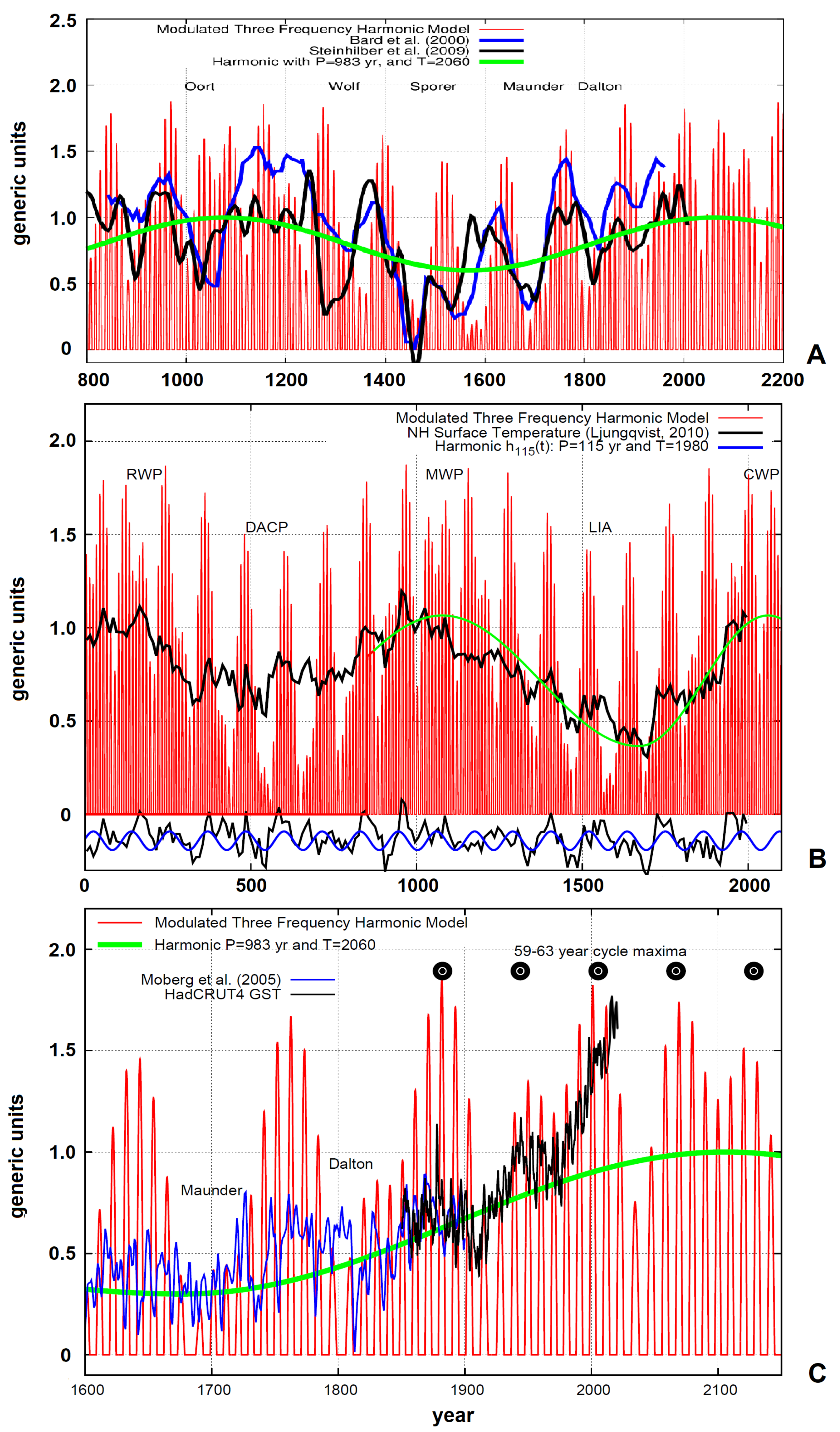
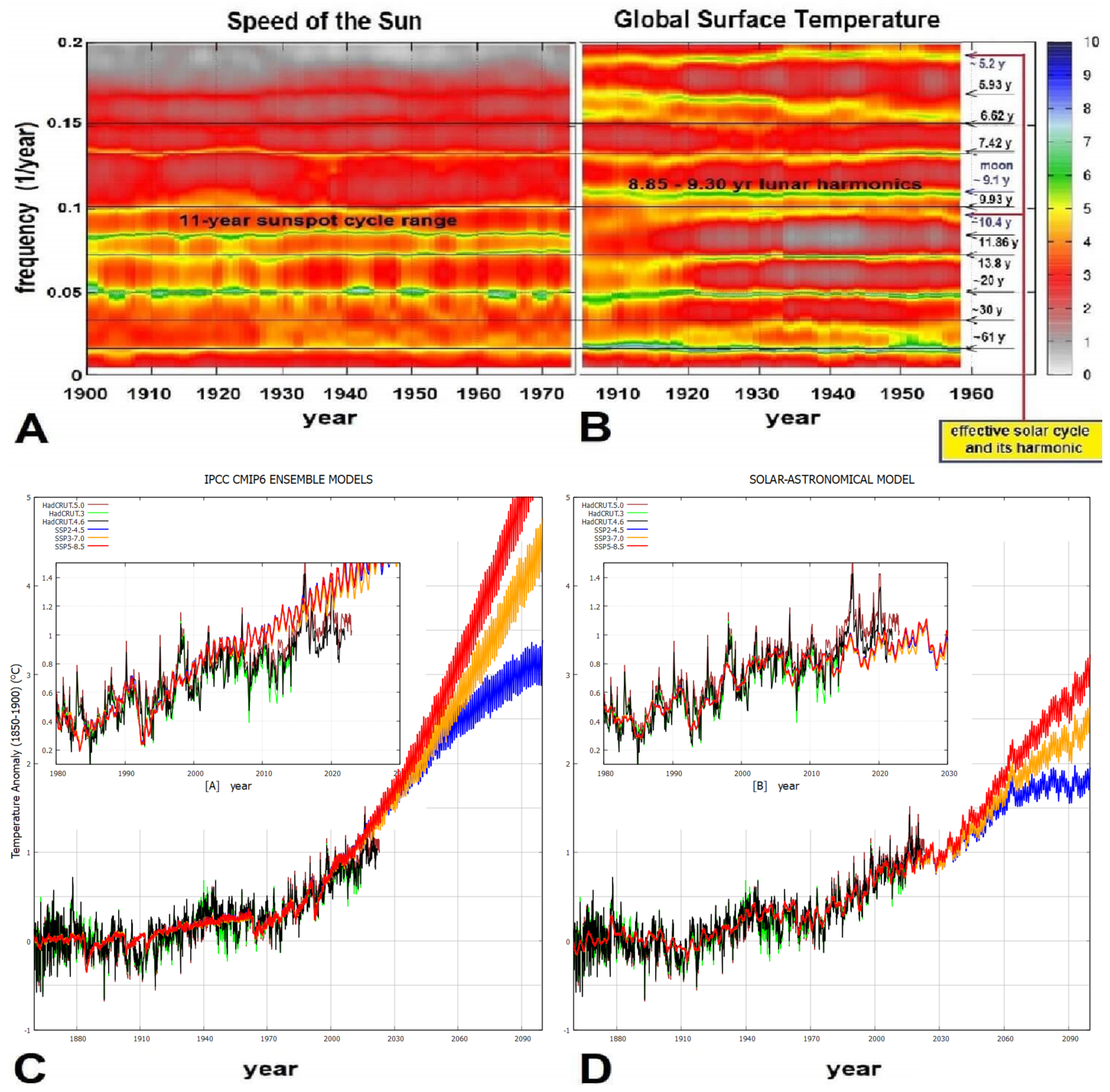
3.3. Evidences for Interannual and Multidecadal Planetary Periods in Global Surface Temperature Records
4. Addressing the Critiques
4.1. How should the Sun’s Wobbling Be Understood?
4.2. The “Homeopathic” Tiny-Tidal Problem
4.3. Rebuttals of the Claims That Planetary Harmonics Are Incompatible with Solar Activity Cycles
4.4. A Brief Response to Some Unscientific Critiques
5. Conclusions
Author Contributions
Funding
Data Availability Statement
Acknowledgments
Conflicts of Interest
References
- Vinós, J. Nature Unbound III—Holocene Climate Variability (Part B). Posted on 28 May 2017. Available online: https://judithcurry.com/2017/05/28/nature-unbound-iii-holocene-climate-variability-part-b/ (accessed on 24 March 2023).
- Shaviv, N.J.; Veizer, J. Celestial driver of Phanerozoic climate? GSA Today 2003, 13, 4. [Google Scholar] [CrossRef]
- Svensmark, H. Cosmoclimatology: A new theory emerges. Astron. Geophys. 2007, 48, 1.18–1.24. [Google Scholar] [CrossRef] [Green Version]
- Rampino, M.R.; Caldeira, K. A 32-million year cycle detected in sea-level fluctuations over the last 545 Myr. Geosci. Front. 2020, 11, 2061–2065. [Google Scholar] [CrossRef]
- Laskar, J.; Robutel, P.; Joutel, F.; Gastineau, M.; Correia, A.C.M.; Levrard, B. A long-term numerical solution for the insolation quantities of the Earth. Astron. Astrophys. 2004, 428, 261–285. [Google Scholar] [CrossRef] [Green Version]
- Scafetta, N.; Milani, F.; Bianchini, A.; Ortolani, S. On the astronomical origin of the Hallstatt oscillation found in radiocarbon and climate records throughout the Holocene. Earth-Sci. Rev. 2016, 162, 24–43. [Google Scholar] [CrossRef] [Green Version]
- Scafetta, N. Solar Oscillations and the Orbital Invariant Inequalities of the Solar System. Sol. Phys. 2020, 295, 33. [Google Scholar] [CrossRef]
- Cionco, R.G.; Soon, W.W.H. Short-term orbital forcing: A quasi-review and a reappraisal of realistic boundary conditions for climate modeling. Earth-Sci. Rev. 2017, 166, 206–222. [Google Scholar] [CrossRef] [Green Version]
- Cionco, R.G.; Kudryavtsev, S.M.; Soon, W.W.H. Possible Origin of Some Periodicities Detected in Solar-Terrestrial Studies: Earth’s Orbital Movements. Earth Space Sci. 2021, 8, e2021EA001805. [Google Scholar] [CrossRef]
- Scafetta, N.; Milani, F.; Bianchini, A. Multiscale Analysis of the Instantaneous Eccentricity Oscillations of the Planets of the Solar System from 13,000 BC to 17,000 AD. Astron. Lett. 2019, 45, 778–790. [Google Scholar] [CrossRef]
- Scafetta, N. Reconstruction of the Interannual to Millennial Scale Patterns of the Global Surface Temperature. Atmosphere 2021, 12, 147. [Google Scholar] [CrossRef]
- Scafetta, N. Empirical evidence for a celestial origin of the climate oscillations and its implications. J. Atmos. Sol.-Terr. Phys. 2010, 72, 951–970. [Google Scholar] [CrossRef] [Green Version]
- Svensmark, H. Supernova rates and burial of organic matter. Geophys. Res. Lett. 2021, 48, e2021GL096376. [Google Scholar] [CrossRef]
- Hansen, J.; Sato, M.; Russell, G.; Kharecha, P. Climate sensitivity, sea level and atmospheric carbon dioxide. Philos. Trans. R. Soc. A Math. Phys. Eng. Sci. 2013, 371, 20120294. [Google Scholar] [CrossRef] [PubMed]
- Jouzel, J.; Masson-Delmotte, V.; Cattani, O.; Dreyfus, G.; Falourd, S.; Hoffmann, G.; Minster, B.; Nouet, J.; Barnola, J.M.; Chappellaz, J.; et al. Orbital and Millennial Antarctic Climate Variability over the Past 800,000 Years. Science 2007, 317, 793–796. [Google Scholar] [CrossRef] [PubMed] [Green Version]
- Lisiecki, L.E.; Raymo, M.E. A Pliocene-Pleistocene stack of 57 globally distributed benthic δ18O records. Paleoceanography 2005, 20, PA1003. [Google Scholar] [CrossRef] [Green Version]
- Marcott, S.A.; Shakun, J.D.; Clark, P.U.; Mix, A.C. A Reconstruction of Regional and Global Temperature for the Past 11,300 Years. Science 2013, 339, 1198–1201. [Google Scholar] [CrossRef] [Green Version]
- North Greenland Ice Core Project members: High-resolution record of Northern Hemisphere climate extending into the last interglacial period. Nature 2004, 431, 147–151. [CrossRef] [Green Version]
- Rohde, R.A.; Hausfather, Z. The Berkeley Earth Land/Ocean Temperature Record. Earth Syst. Sci. Data 2020, 12, 3469–3479. [Google Scholar] [CrossRef]
- Royer, D.L.; Berner, R.A.; Montañez, I.P.; Tabor, N.J.; Beerling, D.J. CO2 as a primary driver of Phanerozoic climate. GSA Today 2004, 14, 4. [Google Scholar] [CrossRef]
- Zachos, J.C.; Dickens, G.R.; Zeebe, R.E. An early Cenozoic perspective on greenhouse warming and carbon-cycle dynamics. Nature 2008, 451, 279–283. [Google Scholar] [CrossRef] [Green Version]
- Berner, R.A. GEOCARB III: A revised model of atmospheric CO2 over Phanerozoic time. Am. J. Sci. 2001, 301, 182–204. [Google Scholar] [CrossRef]
- Davis, W. The Relationship between Atmospheric Carbon Dioxide Concentration and Global Temperature for the Last 425 Million Years. Climate 2017, 5, 76. [Google Scholar] [CrossRef] [Green Version]
- Petit, J.R.; Jouzel, J.; Raynaud, D.; Barkov, N.I.; Barnola, J.M.; Basile, I.; Bender, M.; Chappellaz, J.; Davis, M.; Delaygue, G.; et al. Climate and atmospheric history of the past 420,000 years from the Vostok ice core, Antarctica. Nature 1999, 399, 429–436. [Google Scholar] [CrossRef] [Green Version]
- Shakun, J.D.; Clark, P.U.; He, F.; Marcott, S.A.; Mix, A.C.; Liu, Z.; Otto-Bliesner, B.; Schmittner, A.; Bard, E. Global warming preceded by increasing carbon dioxide concentrations during the last deglaciation. Nature 2012, 484, 49–54. [Google Scholar] [CrossRef]
- Scafetta, N.; Bianchini, A. The Planetary Theory of Solar Activity Variability: A Review. Front. Astron. Space Sci. 2022, 9. [Google Scholar] [CrossRef]
- Wolf, R. Extract of a Letter from Prof. R. Wolf, of Zurich, to Mr. Carrington, dated Jan. 12, 1859. Mon. Not. R. Astron. Soc. 1859, 19, 85–86. [Google Scholar] [CrossRef] [Green Version]
- Malburet, J. Sur la période des maxima d’activité solaire. Comptes Rendus Geosci. 2019, 351, 351–354. [Google Scholar] [CrossRef]
- Malburet, J. Sur la cause de la périodicité des tâches solaires. L’Astronomie 1925, 39, 503–515. [Google Scholar]
- Wood, K.D. Physical Sciences: Sunspots and Planets. Nature 1972, 240, 91–93. [Google Scholar] [CrossRef]
- Charbonneau, P. The planetary hypothesis revived. Nature 2013, 493, 613–614. [Google Scholar] [CrossRef]
- Fedorov, V.M.; Frolov, D.M.; Herrera, V.M.N.V.; Soon, W.H.; Cionco, R.G. Role of the Radiation Factor in Global Climatic Events of the Late Holocene. Izv. Atmos. Ocean. Phys. 2021, 57, 1239–1253. [Google Scholar] [CrossRef]
- Soon, W.; Legates, D.R. Solar irradiance modulation of Equator-to-Pole (Arctic) temperature gradients: Empirical evidence for climate variation on multi-decadal timescales. J. Atmos. Sol.-Terr. Phys. 2013, 93, 45–56. [Google Scholar] [CrossRef]
- Neff, U.; Burns, S.J.; Mangini, A.; Mudelsee, M.; Fleitmann, D.; Matter, A. Strong coherence between solar variability and the monsoon in Oman between 9 and 6kyr ago. Nature 2001, 411, 290–293. [Google Scholar] [CrossRef] [PubMed]
- Ogurtsov, M.G.; Nagovitsyn, Y.A.; Kocharov, G.E.; Jungner, H. Long-Period Cycles of the Sun’s Activity Recorded in Direct Solar Data and Proxies. Sol. Phys. 2002, 211, 371–394. [Google Scholar] [CrossRef]
- Scafetta, N.; Grigolini, P.; Imholt, T.; Roberts, J.; West, B.J. Solar turbulence in earth’s global and regional temperature anomalies. Phys. Rev. E 2004, 69, 26303. [Google Scholar] [CrossRef] [PubMed] [Green Version]
- Scafetta, N. Multi-scale harmonic model for solar and climate cyclical variation throughout the Holocene based on Jupiter–Saturn tidal frequencies plus the 11-year solar dynamo cycle. J. Atmos. Sol.-Terr. Phys. 2012, 80, 296–311. [Google Scholar] [CrossRef] [Green Version]
- Steinhilber, F.; Abreu, J.A.; Beer, J.; Brunner, I.; Christl, M.; Fischer, H.; Heikkilä, U.; Kubik, P.W.; Mann, M.; McCracken, K.G.; et al. 9400 years of cosmic radiation and solar activity from ice cores and tree rings. Proc. Natl. Acad. Sci. USA 2012, 109, 5967–5971. [Google Scholar] [CrossRef] [Green Version]
- Kerr, R.A. A Variable Sun Paces Millennial Climate. Science 2001, 294, 1431–1433. [Google Scholar] [CrossRef] [PubMed] [Green Version]
- Kirkby, J. Cosmic Rays and Climate. Surv. Geophys. 2007, 28, 333–375. [Google Scholar] [CrossRef]
- Easterbrook, D.J. Solar Magnetic Cause of Climate Changes and Origin of the Ice Ages; Amazon Distribution: Bellingham, WA, USA, 2019. [Google Scholar]
- Hoyt, D.V.; Schatten, K.H. A discussion of plausible solar irradiance variations, 1700–1992. J. Geophys. Res. Space Phys. 1993, 98, 18895–18906. [Google Scholar] [CrossRef] [Green Version]
- Hoyt, D.V.; Schatten, K.H. The Role of the Sun in Climate Change; Oxford University Press,: Oxford, UK, 1997. [Google Scholar]
- Roy, I. Solar cyclic variability can modulate winter Arctic climate. Sci. Rep. 2018, 8, 4864. [Google Scholar] [CrossRef] [PubMed] [Green Version]
- Dobrica, V.; Pirloaga, R.; Stefan, C.; Demetrescu, C. Inferring geoeffective solar variability signature in stratospheric and tropospheric Northern Hemisphere temperatures. J. Atmos. Sol.-Terr. Phys. 2018, 180, 137–147. [Google Scholar] [CrossRef]
- Mörner, N.A. Planetary beat and solar-terrestrial responses. Pattern Recognit. Phys. 2013, 1, 107–116. [Google Scholar] [CrossRef]
- Baidolda, F. Search for Planetary Influences on Solar Activity; Université Paris, Sciences et Lettres: Paris, France, 2017. [Google Scholar]
- Scafetta, N. Discussion on the spectral coherence between planetary, solar and climate oscillations: A reply to some critiques. Astrophys. Space Sci. 2014, 354, 275–299. [Google Scholar] [CrossRef] [Green Version]
- Lean, J.; Beer, J.; Bradley, R. Reconstruction of solar irradiance since 1610: Implications for climate change. Geophys. Res. Lett. 1995, 22, 3195–3198. [Google Scholar] [CrossRef] [Green Version]
- Wang, Y.M.; Lean, J.L.; Sheeley, N.R., Jr. Modeling the Sun’s Magnetic Field and Irradiance since 1713. Astrophys. J. 2005, 625, 522–538. [Google Scholar] [CrossRef]
- Vieira, L.E.A.; Solanki, S.K.; Krivova, N.A.; Usoskin, I. Evolution of the solar irradiance during the Holocene. Astron. Astrophys. 2011, 531, A6. [Google Scholar] [CrossRef] [Green Version]
- Steinhilber, F.; Beer, J.; Fröhlich, C. Total solar irradiance during the Holocene. Geophys. Res. Lett. 2009, 36, 40142. [Google Scholar] [CrossRef] [Green Version]
- Bard, E.; Raisbeck, G.; Yiou, F.; Jouzel, J. Solar irradiance during the last 1200 years based on cosmogenic nuclides. Tellus B Chem. Phys. Meteorol. 2000, 52, 985. [Google Scholar] [CrossRef]
- Egorova, T.; Schmutz, W.; Rozanov, E.; Shapiro, A.I.; Usoskin, I.; Beer, J.; Tagirov, R.V.; Peter, T. Revised historical solar irradiance forcing. Astron. Astrophys. 2018, 615, A85. [Google Scholar] [CrossRef] [Green Version]
- Shapiro, A.I.; Schmutz, W.; Rozanov, E.; Schoell, M.; Haberreiter, M.; Shapiro, A.V.; Nyeki, S. A new approach to the long-term reconstruction of the solar irradiance leads to large historical solar forcing. Astron. Astrophys. 2011, 529, A67. [Google Scholar] [CrossRef] [Green Version]
- Coddington, O.; Lean, J.L.; Pilewskie, P.; Snow, M.; Lindholm, D. A Solar Irradiance Climate Data Record. Bull. Am. Meteorol. Soc. 2016, 97, 1265–1282. [Google Scholar] [CrossRef]
- Yeo, K.L.; Solanki, S.K.; Krivova, N.A.; Rempel, M.; Anusha, L.S.; Shapiro, A.I.; Tagirov, R.V.; Witzke, V. The Dimmest State of the Sun. Geophys. Res. Lett. 2020, 47, e2020GL090243. [Google Scholar] [CrossRef]
- Schmutz, W.K. Changes in the Total Solar Irradiance and climatic effects. J. Space Weather. Space Clim. 2021, 11, 40. [Google Scholar] [CrossRef]
- McCracken, K.G.; Beer, J.; Steinhilber, F.; Abreu, J. A Phenomenological Study of the Cosmic Ray Variations over the Past 9400 Years, and Their Implications Regarding Solar Activity and the Solar Dynamo. Sol. Phys. 2013, 286, 609–627. [Google Scholar] [CrossRef]
- Eddy, J.A. Climate and the changing sun. Clim. Chang. 1977, 1, 173–190. [Google Scholar] [CrossRef]
- Eichler, A.; Olivier, S.; Henderson, K.; Laube, A.; Beer, J.; Papina, T.; Gäggeler, H.W.; Schwikowski, M. Temperature response in the Altai region lags solar forcing. Geophys. Res. Lett. 2009, 36, 35930. [Google Scholar] [CrossRef] [Green Version]
- Vahrenholt, F.; Lüning, S. The Neglected Sun—Why the Sun Precludes Climate Catastrophe; Stacey International: London, UK, 2013. [Google Scholar]
- Willson, R.C.; Mordvinov, A.V. Secular total solar irradiance trend during solar cycles 21–23. Geophys. Res. Lett. 2003, 30, 1199. [Google Scholar] [CrossRef] [Green Version]
- Fröhlich, C. Total Solar Irradiance Observations. Surv. Geophys. 2012, 33, 453–473. [Google Scholar] [CrossRef]
- Scafetta, N.; Willson, R.; Lee, J.; Wu, D. Modeling Quiet Solar Luminosity Variability from TSI Satellite Measurements and Proxy Models during 1980–2018. Remote Sens. 2019, 11, 2569. [Google Scholar] [CrossRef] [Green Version]
- Montillet, J.P.; Finsterle, W.; Kermarrec, G.; Sikonja, R.; Haberreiter, M.; Schmutz, W.; de Wit, T.D. Data Fusion of Total Solar Irradiance Composite Time Series Using 41 Years of Satellite Measurements. J. Geophys. Res. Atmos. 2022, 127, e2021JD036146. [Google Scholar] [CrossRef]
- De Wit, T.D.; Kopp, G.; Fröhlich, C.; Schöll, M. Methodology to create a new total solar irradiance record: Making a composite out of multiple data records. Geophys. Res. Lett. 2017, 44, 1196–1203. [Google Scholar] [CrossRef] [Green Version]
- Scafetta, N.; Willson, R.C. ACRIM total solar irradiance satellite composite validation versus TSI proxy models. Astrophys. Space Sci. 2014, 350, 421–442. [Google Scholar] [CrossRef] [Green Version]
- Krivova, N.A.; Solanki, S.K.; Wenzler, T. ACRIM-gap and total solar irradiance revisited: Is there a secular trend between 1986 and 1996? Geophys. Res. Lett. 2009, 36, 40707. [Google Scholar] [CrossRef] [Green Version]
- Yeo, K.L.; Krivova, N.A.; Solanki, S.K.; Glassmeier, K.H. Reconstruction of total and spectral solar irradiance from 1974 to 2013 based on KPVT, SoHO/MDI, and SDO/HMI observations. Astron. Astrophys. 2014, 570, A85. [Google Scholar] [CrossRef] [Green Version]
- Matthes, K.; Funke, B.; Andersson, M.E.; Barnard, L.; Beer, J.; Charbonneau, P.; Clilverd, M.A.; de Wit, T.D.; Haberreiter, M.; Hendry, A.; et al. Solar forcing for CMIP6 (v3.2). Geosci. Model Dev. 2017, 10, 2247–2302. [Google Scholar] [CrossRef] [Green Version]
- Scafetta, N. Empirical analysis of the solar contribution to global mean air surface temperature change. J. Atmos. Sol.-Terr. Phys. 2009, 71, 1916–1923. [Google Scholar] [CrossRef] [Green Version]
- Connolly, R.; Soon, W.; Connolly, M.; Baliunas, S.; Berglund, J.; Butler, C.J.; Cionco, R.G.; Elias, A.G.; Fedorov, V.M.; Harde, H.; et al. How much has the Sun influenced Northern Hemisphere temperature trends? An ongoing debate. Res. Astron. Astrophys. 2021, 21, 131. [Google Scholar] [CrossRef]
- Scafetta, N. Does the Sun work as a nuclear fusion amplifier of planetary tidal forcing? A proposal for a physical mechanism based on the mass-luminosity relation. J. Atmos. Sol.-Terr. Phys. 2012, 81–82, 27–40. [Google Scholar] [CrossRef] [Green Version]
- Bendandi, R. Un Principio Fondamentale Dell’Universo; Osservatorio Bendandi: Faenza, Italy, 1931. [Google Scholar]
- Hung, C.C. Apparent Relations Between Solar Activity and Solar Tides Caused by the Planets. NASA Rep. 2007, TM-2007-214817, 1–34. [Google Scholar]
- Okhlopkov, V.P. The gravitational influence of Venus, the Earth, and Jupiter on the 11-year cycle of solar activity. Mosc. Univ. Phys. Bull. 2016, 71, 440–446. [Google Scholar] [CrossRef]
- Okhlopkov, V.P. 11-Year Index of Linear Configurations of Venus, Earth, and Jupiter and Solar Activity. Geomagn. Aeron. 2020, 60, 381–390. [Google Scholar] [CrossRef]
- Stefani, F.; Giesecke, A.; Weber, N.; Weier, T. Synchronized Helicity Oscillations: A Link Between Planetary Tides and the Solar Cycle? Sol. Phys. 2016, 291, 2197–2212. [Google Scholar] [CrossRef] [Green Version]
- Stefani, F.; Giesecke, A.; Weber, N.; Weier, T. On the Synchronizability of Tayler–Spruit and Babcock–Leighton Type Dynamos. Sol. Phys. 2018, 293, 12. [Google Scholar] [CrossRef] [Green Version]
- Stefani, F.; Giesecke, A.; Weier, T. A Model of a Tidally Synchronized Solar Dynamo. Sol. Phys. 2019, 294, 60. [Google Scholar] [CrossRef] [Green Version]
- Tattersall, R. The Hum: Log-normal distribution and planetary–solar resonance. Pattern Recognit. Phys. 2013, 1, 185–198. [Google Scholar] [CrossRef]
- Wilson, I.R.G. The Venus–Earth–Jupiter spin–orbit coupling model. Pattern Recognit. Phys. 2013, 1, 147–158. [Google Scholar] [CrossRef] [Green Version]
- Scafetta, N. Comment on “Tidally Synchronized Solar Dynamo: A Rebuttal” by Nataf (Solar Phys. 297, 107, 2022). Sol. Phys. 2023, 298, 24. [Google Scholar] [CrossRef]
- Scafetta, N. Discussion on climate oscillations: CMIP5 general circulation models versus a semi-empirical harmonic model based on astronomical cycles. Earth-Sci. Rev. 2013, 126, 321–357. [Google Scholar] [CrossRef] [Green Version]
- Okal, E.; Anderson, D.L. On the planetary theory of sunspots. Nature 1975, 253, 511–513. [Google Scholar] [CrossRef]
- Nataf, H.C. Tidally Synchronized Solar Dynamo: A Rebuttal. Sol. Phys. 2022, 297, 107. [Google Scholar] [CrossRef]
- Tan, B.; Cheng, Z. The mid-term and long-term solar quasi-periodic cycles and the possible relationship with planetary motions. Astrophys. Space Sci. 2012, 343, 511–521. [Google Scholar] [CrossRef] [Green Version]
- Scafetta, N. The complex planetary synchronization structure of the solar system. Pattern Recognit. Phys. 2014, 2, 1–19. [Google Scholar] [CrossRef] [Green Version]
- Scafetta, N.; Milani, F.; Bianchini, A. A 60-Year Cycle in the Meteorite Fall Frequency Suggests a Possible Interplanetary Dust Forcing of the Earth’s Climate Driven by Planetary Oscillations. Geophys. Res. Lett. 2020, 47, e2020GL089954. [Google Scholar] [CrossRef]
- Bigg, E.K. Influence of the planet Mercury on sunspots. Astron. J. 1967, 72, 463. [Google Scholar] [CrossRef]
- Scafetta, N.; Willson, R.C. Empirical evidences for a planetary modulation of total solar irradiance and the TSI signature of the 1.09-year Earth-Jupiter conjunction cycle. Astrophys. Space Sci. 2013, 348, 25–39. [Google Scholar] [CrossRef] [Green Version]
- Scafetta, N.; Willson, R.C. Multiscale comparative spectral analysis of satellite total solar irradiance measurements from 2003 to 2013 reveals a planetary modulation of solar activity and its nonlinear dependence on the 11 yr solar cycle. Pattern Recognit. Phys. 2013, 1, 123–133. [Google Scholar] [CrossRef] [Green Version]
- Snodgrass, H.B.; Ulrich, R.K. Rotation of Doppler features in the solar photosphere. Astrophys. J. 1990, 351, 309. [Google Scholar] [CrossRef]
- Shkolnik, E.; Walker, G.A.H.; Bohlender, D.A. Evidence for Planet-induced Chromospheric Activity on HD 179949. Astrophys. J. 2003, 597, 1092–1096. [Google Scholar] [CrossRef] [Green Version]
- Shkolnik, E.; Walker, G.A.H.; Bohlender, D.A.; Gu, P.G.; Kurster, M. Hot Jupiters and Hot Spots: The Short- and Long-Term Chromospheric Activity on Stars with Giant Planets. Astrophys. J. 2005, 622, 1075–1090. [Google Scholar] [CrossRef]
- Pizzella, G. Emission of cosmic rays from Jupiter: Magnetospheres as possible sources of cosmic rays. Eur. Phys. J. C 2018, 78, 1–7. [Google Scholar] [CrossRef] [Green Version]
- Salvador, R.J. A mathematical model of the sunspot cycle for the past 1000 yr. Pattern Recognit. Phys. 2013, 1, 117–122. [Google Scholar] [CrossRef]
- Mörner, N.A. The Approaching New Grand Solar Minimum and Little Ice Age Climate Conditions. Nat. Sci. 2015, 7, 510–518. [Google Scholar] [CrossRef] [Green Version]
- Courtillot, V.; Lopes, F.; Mouël, J.L.L. On the Prediction of Solar Cycles. Sol. Phys. 2021, 296, 1–23. [Google Scholar] [CrossRef]
- Ljungqvist, F.C. A new reconstruction of temperature variability in the extra-tropical northern hemisphere during the last two millennia. Geogr. Ann. Ser. A Phys. Geogr. 2010, 92, 339–351. [Google Scholar] [CrossRef]
- Morice, C.P.; Kennedy, J.J.; Rayner, N.A.; Jones, P.D. Quantifying uncertainties in global and regional temperature change using an ensemble of observational estimates: The HadCRUT4 data set. J. Geophys. Res. Atmos. 2012, 117, 17187. [Google Scholar] [CrossRef] [Green Version]
- Moberg, A.; Sonechkin, D.M.; Holmgren, K.; Datsenko, N.M.; Karlén, W. Highly variable Northern Hemisphere temperatures reconstructed from low- and high-resolution proxy data. Nature 2005, 433, 613–617. [Google Scholar] [CrossRef]
- Kutschera, W.; Patzelt, G.; Steier, P.; Wild, E.M. The Tyrolean Iceman and His Glacial Environment During the Holocene. Radiocarbon 2017, 59, 395–405. [Google Scholar] [CrossRef]
- Alley, R.B. GISP2—Temperature Reconstruction and Accumulation Data. In IGBP PAGES/World Data Center for Paleoclimatology Data Contribution Series 2004-013; NOAA National Centers for Environmental Information: Asheville, NC, USA, 2004. [Google Scholar] [CrossRef]
- Cauquoin, A.; Raisbeck, G.M.; Jouzel, J.; Bard, E. No evidence for planetary influence on solar activity 330,000 years ago. Astron. Astrophys. 2014, 561, A132. [Google Scholar] [CrossRef] [Green Version]
- Smythe, C.M.; Eddy, J.A. Planetary tides during the Maunder Sunspot Minimum. Nature 1977, 266, 434–435. [Google Scholar] [CrossRef]
- Poluianov, S.; Usoskin, I. Critical Analysis of a Hypothesis of the Planetary Tidal Influence on Solar Activity. Sol. Phys. 2014, 289, 2333–2342. [Google Scholar] [CrossRef] [Green Version]
- Abreu, J.A.; Albert, C.; Beer, J.; Ferriz-Mas, A.; McCracken, K.G.; Steinhilber, F. Response to: “Critical Analysis of a Hypothesis of the Planetary Tidal Influence on Solar Activity” by S. Poluianov and I. Usoskin. Sol. Phys. 2014, 289, 2343–2344. [Google Scholar] [CrossRef]
- Scafetta, N. High resolution coherence analysis between planetary and climate oscillations. Adv. Space Res. 2016, 57, 2121–2135. [Google Scholar] [CrossRef]
- Reimer, P.J.; Baillie, M.; Bard, E.; Bayliss, A.; Beck, J.W.; Bertrand, C.J.H.; Blackwell, P.G.; Buck, C.E.; Burr, G.S.; Cutler, K.B.; et al. Intcal04 Terrestrial Radiocarbon Age Calibration, 0–26 Cal Kyr BP. Radiocarbon 2004, 46, 1029–1058. [Google Scholar] [CrossRef] [Green Version]
- Charvátová, I. Can origin of the 2400-year cycle of solar activity be caused by solar inertial motion? Ann. Geophys. 2000, 18, 399–405. [Google Scholar] [CrossRef]
- Cionco, R.G.; Pavlov, D.A. Solar barycentric dynamics from a new solar-planetary ephemeris. Astron. Astrophys. 2018, 615, A153. [Google Scholar] [CrossRef]
- Fairbridge, R.W.; Shirley, J.H. Prolonged minima and the 179-yr cycle of the solar inertial motion. Sol. Phys. 1987, 110, 191–210. [Google Scholar] [CrossRef]
- McCracken, K.G.; Beer, J.; Steinhilber, F. Evidence for Planetary Forcing of the Cosmic Ray Intensity and Solar Activity Throughout the Past 9400 Years. Sol. Phys. 2014, 289, 3207–3229. [Google Scholar] [CrossRef]
- Usoskin, I.G.; Gallet, Y.; Lopes, F.; Kovaltsov, G.A.; Hulot, G. Solar activity during the Holocene: The Hallstatt cycle and its consequence for grand minima and maxima. Astron. Astrophys. 2016, 587, A150. [Google Scholar] [CrossRef] [Green Version]
- Bray, J.R. Glaciation and Solar Activity since the Fifth Century BC and the Solar Cycle. Nature 1968, 220, 672–674. [Google Scholar] [CrossRef]
- Vasiliev, S.S.; Dergachev, V.A. The 2400-year cycle in atmospheric radiocarbon concentration: Bispectrum of 14C data over the last 8000 years. Ann. Geophys. 2002, 20, 115–120. [Google Scholar] [CrossRef] [Green Version]
- Bertolucci, S.; Zioutas, K.; Hofmann, S.; Maroudas, M. The Sun and its Planets as detectors for invisible matter. Phys. Dark Univ. 2017, 17, 13–21. [Google Scholar] [CrossRef]
- Petrakou, E. Planetary statistics and forecasting for solar flares. Adv. Space Res. 2021, 68, 2963–2973. [Google Scholar] [CrossRef]
- Scafetta, N. A shared frequency set between the historical mid-latitude aurora records and the global surface temperature. J. Atmos. Sol.-Terr. Phys. 2012, 74, 145–163. [Google Scholar] [CrossRef] [Green Version]
- Scafetta, N.; Willson, R.C. Planetary harmonics in the historical Hungarian aurora record (1523–1960). Planet. Space Sci. 2013, 78, 38–44. [Google Scholar] [CrossRef] [Green Version]
- Sharp, G.J. Are Uranus and Neptune Responsible for Solar Grand Minima and Solar Cycle Modulation? Int. J. Astron. Astrophys. 2013, 3, 260–273. [Google Scholar] [CrossRef] [Green Version]
- Abreu, J.A.; Beer, J.; Ferriz-Mas, A.; McCracken, K.G.; Steinhilber, F. Is there a planetary influence on solar activity? Astron. Astrophys. 2012, 548, A88. [Google Scholar] [CrossRef] [Green Version]
- Lopes, F.; Mouël, J.L.; Courtillot, V.; Gibert, D. On the shoulders of Laplace. Phys. Earth Planet. Inter. 2021, 316, 106693. [Google Scholar] [CrossRef]
- Scafetta, N. Reply on Comment on “High resolution coherence analysis between planetary and climate oscillations” by S. Holm. Adv. Space Res. 2018, 62, 334–342. [Google Scholar] [CrossRef] [Green Version]
- Brohan, P.; Kennedy, J.J.; Harris, I.; Tett, S.F.B.; Jones, P.D. Uncertainty estimates in regional and global observed temperature changes: A new data set from 1850. J. Geophys. Res. 2006, 111, 6548. [Google Scholar] [CrossRef] [Green Version]
- Scafetta, N. Testing an astronomically based decadal-scale empirical harmonic climate model versus the IPCC (2007) general circulation climate models. J. Atmos. Sol.-Terr. Phys. 2012, 80, 124–137. [Google Scholar] [CrossRef] [Green Version]
- Keeling, C.D.; Whorf, T.P. The 1800-year oceanic tidal cycle: A possible cause of rapid climate change. Proc. Natl. Acad. Sci. USA 2000, 97, 3814–3819. [Google Scholar] [CrossRef] [PubMed] [Green Version]
- Morice, C.P.; Kennedy, J.J.; Rayner, N.A.; Winn, J.P.; Hogan, E.; Killick, R.E.; Dunn, R.J.H.; Osborn, T.J.; Jones, P.D.; Simpson, I.R. An Updated Assessment of Near-Surface Temperature Change From 1850: The HadCRUT5 Data Set. J. Geophys. Res. Atmos. 2021, 126, e2019JD032361. [Google Scholar] [CrossRef]
- Scafetta, N.; Humlum, O.; Solheim, J.E.; Stordahl, K. Comment on “The influence of planetary attractions on the solar tachocline” by Callebaut, de Jager and Duhau. J. Atmos. Sol.-Terr. Phys. 2013, 102, 368–371. [Google Scholar] [CrossRef] [Green Version]
- Stocker, T.F.; Qin, D.; Plattner, G.-K.; Tignor, M.; Allen, S.K.; Boschung, J.; Nauels, A.; Xia, Y.; Bex, V.; Midgley, P.M. (Eds.) Climate Change 2013 The Physical Science Basis: Assessment Working Group I Contribution to the IPCC Fifth Assessment Report; Cambridge University Press: Cambridge, UK, 2014. [Google Scholar]
- Masson-Delmotte, V.; Zhai, P.; Pirani, A.; Connors, S.L.; Péan, C.; Berger, S.; Caud, N.; Chen, Y.; Goldfarb, L.; Gomis, M.I.; et al. (Eds.) Climate Change 2021 The Physical Science Basis: Assessment Working Group I Contribution to the IPCC Sixth Assessment Report; Cambridge University Press: Cambridge, UK, 2021. [Google Scholar]
- Jager, C.D.; Nieuwenhuizen, A.; Duhau, S. The relation between the average northern hemisphere ground temperature and solar equatorial and polar magnetic activity. Phys. Astron. Int. J. 2018, 2, 175–185. [Google Scholar] [CrossRef]
- Richards, M.T.; Rogers, M.L.; Richards, D.S.P. Long-term Variability in the Length of the Solar Cycle. Publ. Astron. Soc. Pac. 2009, 121, 797–809. [Google Scholar] [CrossRef] [Green Version]
- Eyring, V.; Bony, S.; Meehl, G.A.; Senior, C.A.; Stevens, B.; Stouffer, R.J.; Taylor, K.E. Overview of the Coupled Model Intercomparison Project Phase 6 (CMIP6) experimental design and organization. Geosci. Model Dev. 2016, 9, 1937–1958. [Google Scholar] [CrossRef] [Green Version]
- Cionco, R.G.; Compagnucci, R.H. Dynamical characterization of the last prolonged solar minima. Adv. Space Res. 2012, 50, 1434–1444. [Google Scholar] [CrossRef] [Green Version]
- Cionco, R.G.; Soon, W. A phenomenological study of the timing of solar activity minima of the last millennium through a physical modeling of the Sun-Planets Interaction. New Astron. 2015, 34, 164–171. [Google Scholar] [CrossRef]
- Yndestad, H.; Solheim, J.E. The influence of solar system oscillation on the variability of the total solar irradiance. New Astron. 2017, 51, 135–152. [Google Scholar] [CrossRef] [Green Version]
- Zharkova, V.V.; Shepherd, S.J.; Zharkov, S.I.; Popova, E. RETRACTED ARTICLE: Oscillations of the baseline of solar magnetic field and solar irradiance on a millennial timescale. Sci. Rep. 2019, 9, 9197. [Google Scholar] [CrossRef] [PubMed] [Green Version]
- Charbonneau, P. Dynamo models of the solar cycle. Living Rev. Sol. Phys. 2020, 17, 1–104. [Google Scholar] [CrossRef]
- Jager, C.D.; Versteegh, G.J.M. Do Planetary Motions Drive Solar Variability? Sol. Phys. 2005, 229, 175–179. [Google Scholar] [CrossRef]
- Callebaut, D.K.; de Jager, C.; Duhau, S. The influence of planetary attractions on the solar tachocline. J. Atmos. -Sol.-Terr. Phys. 2012, 80, 73–78. [Google Scholar] [CrossRef]
- Charbonneau, P. External Forcing of the Solar Dynamo. Front. Astron. Space Sci. 2022, 9, 48. [Google Scholar] [CrossRef]
- Wolff, C.L.; Patrone, P.N. A New Way that Planets Can Affect the Sun. Sol. Phys. 2010, 266, 227–246. [Google Scholar] [CrossRef] [Green Version]
- Hartlep, T.; Mansour, N. Acoustic Wave Propagation in the Sun; Annual Research Briefs; Center for Turbulence Research: Stanford, CA, USA, 2005; pp. 357–365. Available online: https://web.stanford.edu/group/ctr/ResBriefs05/hartlep.pdf (accessed on 24 March 2023).
- Ahuir, J.; Mathis, S.; Amard, L. Dynamical tide in stellar radiative zones. General formalism and evolution for low-mass stars. Astron. Astrophys. 2021, 651, A3. [Google Scholar] [CrossRef]
- Barker, A.J.; Ogilvie, G.I. On internal wave breaking and tidal dissipation near the centre of a solar-type star. Mon. Not. R. Astron. Soc. 2010, 404, 1849–1868. [Google Scholar] [CrossRef] [Green Version]
- Stefani, F.; Stepanov, R.; Weier, T. Shaken and Stirred: When Bond Meets Suess–de Vries and Gnevyshev–Ohl. Sol. Phys. 2021, 296, 88. [Google Scholar] [CrossRef]
- Chatterjee, P.; Nandy, D.; Choudhuri, A.R. Full-sphere simulations of a circulation-dominated solar dynamo: Exploring the parity issue. Astron. Astrophys. 2004, 427, 1019–1030. [Google Scholar] [CrossRef]
- Jiang, J.; Chatterjee, P.; Choudhuri, A.R. Solar activity forecast with a dynamo model. Mon. Not. R. Astron. Soc. 2007, 381, 1527–1542. [Google Scholar] [CrossRef] [Green Version]
- Pikovsky, A. Synchronization—A Universal Concept in Nonlinear Sciences; Cambridge University Press: Cambridge, UK, 2003. [Google Scholar]
- Lopes, F.; Courtillot, V.; Gibert, D.; Mouël, J.L.L. On Two Formulations of Polar Motion and Identification of Its Sources. Geosciences 2022, 12, 398. [Google Scholar] [CrossRef]
- Lopes, F.; Courtillot, V.; Gibert, D.; Mouël, J.L.L. Extending the Range of Milankovic Cycles and Resulting Global Temperature Variations to Shorter Periods (1–100 Year Range). Geosciences 2022, 12, 448. [Google Scholar] [CrossRef]
- Callebaut, D.; de Jager, C.; Duhau, S. Reply to “The influence of planetary attractions on the solar tachocline” by N. Scafetta, O. Humlum, J.E. Solheim, K. Stordahl. J. Atmos. Sol.-Terr. Phys. 2013, 102, 372. [Google Scholar] [CrossRef]
- Nataf, H.C. Response to Comment on “Tidally Synchronized Solar Dynamo: A Rebuttal”. Sol. Phys. 2023, 298, 33. [Google Scholar] [CrossRef]
- Ptolemy. Tetrabiblos, or Quadripartite (2nd Century); Astrology Classics: Bondi, Australia, 2002. [Google Scholar]
- Newton, I. The Principia—Mathematical Principles of Natural Philosophy (1687); Univ. of California Press: Oakland, CA, USA, 1999. [Google Scholar]
- Moldwin, M.B. An Introduction to Space Weather; Cambridge University Press: Cambridge, UK, 2008. [Google Scholar]
- Wegener, A. The Origin of Continents And Oceans (1915); Dover Publications: Mineola, NY, USA, 1966. [Google Scholar]
- Brackenridge, J.; Rossi, M. Johannes Kepler’s on the More Certain Fundamentals of Astrology Prague 1601. Proc. Am. Philos. Soc. 1979, 123, 85–116. [Google Scholar]
- Yamamoto, K.; Burnett, C. Abu Ma’sar on Historical Astrology: The Book of Religions and Dynasties (on the Great Conjunctions); Brill: Leiden, The Netherlands, 2000. [Google Scholar]
- Kepler, J. De Stella Nova in Pede Serpentarii; Typis Pauli Sessii: Pragae, Czech Republic, 1606. [Google Scholar]
- Agnihotri, R.; Dutta, K. Centennial scale variations in monsoonal rainfall (Indian, east equatorial and Chinese monsoons): Manifestations of solar variability. Curr. Sci. 2003, 240, 459–463. [Google Scholar]
- Iyengar, R.N. Monsoon rainfall cycles as depicted in ancient Sanskrit texts. Curr. Sci. 2009, 97, 444–447. [Google Scholar]
- Gupta, S.M. Indian monsoon cycles through the last twelve million years. Earth Sci. India 2010, 3, 248–280. [Google Scholar]


| Mercury | Venus | Earth | Mars | Jupiter | Saturn | Uranus | Neptune | |
| Mercury | 72.3 | 57.9 | 50.4 | 44.9 | 44.3 | 44.1 | 44.0 | |
| Venus | 72.3 | 292.0 | 167.0 | 118.5 | 114.7 | 113.2 | 112.8 | |
| Earth | 57.9 | 292.0 | 390.0 | 199.4 | 189.0 | 184.8 | 183.7 | |
| Mars | 50.4 | 167.0 | 390.0 | 408.2 | 366.9 | 351.4 | 347.5 | |
| Jupiter | 44.9 | 118.5 | 199.4 | 408.2 | 3626.7 | 2522.4 | 2334.3 | |
| Saturn | 44.3 | 114.7 | 189.0 | 366.9 | 3626.7 | 8284.4 | 6550.6 | |
| Uranus | 44.1 | 113.2 | 184.8 | 351.4 | 2522.4 | 8284.4 | 31,300.0 | |
| Neptune | 44.0 | 112.8 | 183.7 | 347.5 | 2334.3 | 6550.6 | 31,300.0 | |
| Mercury | Venus | Earth | Mars | Jupiter | Saturn | Uranus | Neptune | |
| Mercury | 0.198 | 0.159 | 0.138 | 0.123 | 0.121 | 0.121 | 0.121 | |
| Venus | 0.198 | 0.799 | 0.457 | 0.324 | 0.314 | 0.310 | 0.309 | |
| Earth | 0.159 | 0.799 | 1.07 | 0.546 | 0.518 | 0.506 | 0.503 | |
| Mars | 0.138 | 0.457 | 1.07 | 1.12 | 1.00 | 0.962 | 0.951 | |
| Jupiter | 0.123 | 0.324 | 0.546 | 1.12 | 9.93 | 6.91 | 6.39 | |
| Saturn | 0.121 | 0.314 | 0.518 | 1.00 | 9.93 | 22.7 | 17.9 | |
| Uranus | 0.121 | 0.310 | 0.506 | 0.962 | 6.91 | 22.7 | 85.7 | |
| Neptune | 0.121 | 0.309 | 0.503 | 0.951 | 6.39 | 17.9 | 85.7 |
| Mass | Sidereal Orbital Period | Semimajor Axis | Aphelion | Aphelion | Angular Sep. | |
|---|---|---|---|---|---|---|
| (kg) | (Day) | (m) | (m) | |||
| Mercury | 3.30100 | 87.969 | 5.790900 | 6.981800 | 2000.0047 | 143.6 |
| Venus | 4.86730 | 224.701 | 1.082100 | 1.089410 | 2000.2219 | 145.5 |
| Earth | 5.97220 | 365.256 | 1.495980 | 1.521000 | 2000.5087 | 63.6 |
| Mars | 6.41690 | 686.98 | 2.279560 | 2.492610 | 2000.8405 | 37.1 |
| Jupiter | 1.89813 | 4332.589 | 7.784790 | 8.163630 | 2005.2841 | 0.0 |
| Saturn | 5.68320 | 10759.22 | 1.432041 | 1.506527 | 1988.6954 | 9.5 |
| Uranus | 8.68110 | 30685.4 | 2.867043 | 3.001390 | 2009.1554 | 79.8 |
| Neptune | 1.02409 | 60189 | 4.514953 | 4.558857 | 1959.5619 | 92.3 |
| Solar Cycle | Start Minimum | End Minimum | Duration | Maximum | Time of Rise | Average | Spotless |
|---|---|---|---|---|---|---|---|
| # | Date (Y-M) | Date (Y-M) | Years | Date (Y-M) | Year | Spot/Day | Days |
| 1 | 1755-02 | 1766-06 | 11.33 | 1761-06 | 6.33 | 70 | |
| 2 | 1766-06 | 1775-06 | 9.00 | 1769-09 | 3.25 | 99 | |
| 3 | 1775-06 | 1784-09 | 9.25 | 1778-05 | 2.92 | 111 | |
| 4 | 1784-09 | 1798-04 | 13.58 | 1788-02 | 3.42 | 103 | |
| 5 | 1798-04 | 1810-07 | 12.25 | 1805-02 | 6.83 | 38 | |
| 6 | 1810-07 | 1823-05 | 12.83 | 1816-05 | 5.83 | 31 | |
| 7 | 1823-05 | 1833-11 | 10.50 | 1829-11 | 6.50 | 63 | |
| 8 | 1833-11 | 1843-07 | 9.67 | 1837-03 | 3.33 | 112 | |
| 9 | 1843-07 | 1855-12 | 12.42 | 1848-02 | 4.58 | 99 | |
| 10 | 1855-12 | 1867-03 | 11.25 | 1860-02 | 4.17 | 92 | 561 |
| 11 | 1867-03 | 1878-12 | 11.75 | 1870-08 | 3.42 | 89 | 942 |
| 12 | 1878-12 | 1890-03 | 11.25 | 1883-12 | 5.00 | 57 | 872 |
| 13 | 1890-03 | 1902-01 | 11.83 | 1894-01 | 3.83 | 65 | 782 |
| 14 | 1902-01 | 1913-07 | 11.50 | 1906-02 | 4.08 | 54 | 1007 |
| 15 | 1913-07 | 1923-08 | 10.08 | 1917-08 | 4.08 | 73 | 640 |
| 16 | 1923-08 | 1933-09 | 10.08 | 1928-04 | 4.67 | 68 | 514 |
| 17 | 1933-09 | 1944-02 | 10.42 | 1937-04 | 3.58 | 96 | 384 |
| 18 | 1944-02 | 1954-04 | 10.17 | 1947-05 | 3.25 | 109 | 382 |
| 19 | 1954-04 | 1964-10 | 10.50 | 1958-03 | 3.92 | 129 | 337 |
| 20 | 1964-10 | 1976-03 | 11.42 | 1968-11 | 4.08 | 86 | 285 |
| 21 | 1976-03 | 1986-09 | 10.50 | 1979-12 | 3.75 | 111 | 283 |
| 22 | 1986-09 | 1996-08 | 9.92 | 1989-11 | 3.17 | 106 | 257 |
| 23 | 1996-08 | 2008-12 | 12.33 | 2001-11 | 5.25 | 82 | 619 |
| 24 | 2008-12 | 2019-12 | 11.00 | 2014-04 | 5.33 | 49 | 914 |
| 25 | 2019-12 | ||||||
| Average |
| Cycle | ||||
|---|---|---|---|---|
| i | °C | 1/Year | Year | 1/Year |
| 1 | 0.3228 | 0.001316 | 760 | 0.171 |
| 2 | 0.0584 | 0.008696 | 115 | 0.424 |
| 3 | 0.0858 | 0.01639 | 61 | 0.152 |
| 4 | 0.0334 | 0.0500 | 20 | 0.148 |
| 5 | 0.0241 | 0.09615 | 10.4 | 0.020 |
| 6 | 0.0265 | 0.1075 | 9.3 | 0.497 |
| 7 | 0.0216 | 0.1340 | 7.46 | 0.711 |
| 8 | 0.0272 | 0.1666 | 6.00 | 0.617 |
| 9 | 0.0260 | 0.1912 | 5.23 | 0.409 |
| 10 | 0.0326 | 0.2088 | 4.79 | 0.931 |
| 11 | 0.0276 | 0.2754 | 3.63 | 0.767 |
| 12 | 0.0254 | 0.2809 | 3.56 | 0.792 |
| 13 | 0.0247 | 0.3484 | 2.87 | 0.975 |
Disclaimer/Publisher’s Note: The statements, opinions and data contained in all publications are solely those of the individual author(s) and contributor(s) and not of MDPI and/or the editor(s). MDPI and/or the editor(s) disclaim responsibility for any injury to people or property resulting from any ideas, methods, instructions or products referred to in the content. |
© 2023 by the authors. Licensee MDPI, Basel, Switzerland. This article is an open access article distributed under the terms and conditions of the Creative Commons Attribution (CC BY) license (https://creativecommons.org/licenses/by/4.0/).
Share and Cite
Scafetta, N.; Bianchini, A. Overview of the Spectral Coherence between Planetary Resonances and Solar and Climate Oscillations. Climate 2023, 11, 77. https://doi.org/10.3390/cli11040077
Scafetta N, Bianchini A. Overview of the Spectral Coherence between Planetary Resonances and Solar and Climate Oscillations. Climate. 2023; 11(4):77. https://doi.org/10.3390/cli11040077
Chicago/Turabian StyleScafetta, Nicola, and Antonio Bianchini. 2023. "Overview of the Spectral Coherence between Planetary Resonances and Solar and Climate Oscillations" Climate 11, no. 4: 77. https://doi.org/10.3390/cli11040077