
Analysis of Snow Cover in the Sibillini Mountains in Central Italy
by
 ,
,
Matteo Gentilucci
1,* ,
,
Andrea Catorci
2,
Tiziana Panichella
2,
Sara Moscatelli
2,
Younes Hamed
3,4,
Rim Missaoui
3,5 and
Gilberto Pambianchi
1 1
School of Science and Technology, Geology Division, University of Camerino, 62032 Camerino, Italy
2
School of Biosciences and Veterniary Medicine, University of Camerino, 62032 Camerino, Italy
3
Department of Earth Sciences, Laboratory for the Application of Materials to the Environment, Water and Energy (LAM3E), University of Gafsa, Gafsa 2112, Tunisia
4
Department of Earth and Atmospheric Sciences, University of Houston, Science and Research Building 1, 3507 Cullen Blvd, Room 312, Houston, TX 77204, USA
5
Higher Institute of the Sciences and Techniques of Waters of Gabes (ISSTEG), Department of Water Sciences, University of Gabes, Gabes 6072, Tunisia
*
Author to whom correspondence should be addressed.
Climate 2023, 11(3), 72; https://doi.org/10.3390/cli11030072
Submission received: 28 February 2023
/
Revised: 15 March 2023
/
Accepted: 17 March 2023
/
Published: 19 March 2023
(This article belongs to the Special Issue Regional Special Issue: Climate Change in Italy)
Abstract
:Research on solid precipitation and snow cover, especially in mountainous areas, suffers from problems related to the lack of on-site observations and the low reliability of measurements, which is often due to instruments that are not suitable for the environmental conditions. In this context, the study area is the Monti Sibillini National Park, and it is no exception, as it is a mountainous area located in central Italy, where the measurements are scarce and fragmented. The purpose of this research is to provide a characterization of the snow cover with regard to maximum annual snow depth, average snow depth during the snowy period, and days with snow cover on the ground in the Monti Sibillini National Park area, by means of ground weather stations, and also analyzing any trends over the last 30 years. For this research, in order to obtain reliable snow cover data, only data from weather stations equipped with a sonar system and manual weather stations, where the surveyor goes to the site each morning and checks the thickness of the snowpack and records, it were collected. The data were collected from 1 November to 30 April each year for 30 years, from 1991 to 2020; six weather stations were taken into account, while four more were added as of 1 January 2010. The longer period was used to assess possible ongoing trends, which proved to be very heterogeneous in the results, predominantly negative in the case of days with snow cover on the ground, while trends were predominantly positive for maximum annual snow depth and distributed between positive and negative for the average annual snow depth. The shorter period, 2010–2022, on the other hand, ensured the presence of a larger number of weather stations and was used to assess the correlation and presence of clusters between the various weather stations and, consequently, in the study area. Furthermore, in this way, an up-to-date nivometric classification of the study area was obtained (in terms of days with snow on the ground, maximum height of snowpack, and average height of snowpack), filling a gap where there had been no nivometric study in the aforementioned area. The interpolations were processed using geostatistical techniques such as co-kriging with altitude as an independent variable, allowing fairly precise spatialization, analyzing the results of cross-validation. This analysis could be a useful tool for hydrological modeling of the area, as well as having a clear use related to tourism and vegetation, which is extremely influenced by the nivometric variables in its phenology. In addition, this analysis could also be considered a starting point for the calibration of more recent satellite products dedicated to snow cover detection, in order to further improve the compiled climate characterization.
1. Introduction
1.1. Aim of the Study and State of the Art
Snow cover is a variable that has an important influence on vegetation, the hydrological regime, and slope stability, but also on the tourism of an area. Vegetation depends strongly, in certain areas and at certain altitudes, on the melting of the snow pack, which enables the start of the growing season and has a great influence on the germination of both forest species and fruit plants [1,2,3]. Similarly, snow cover affects the hydrological cycle, so much so that it is extremely important for hydrological modeling and water supply, which is reduced due to global warming. This causes early snowmelt, resulting in more frequent winter floods and summer droughts [4,5]. The early melting of snow cover is also detrimental to slope stability, as shown by a piece of recent research in Japan, which showed that an increasing snow cover improves the safety factor and consequently reduces the landslide movement, especially if superficial and small in size [6]. Therefore, it was pointed out that the reduction in snow cover due to global warming is very damaging to the area and even more so if one considers the decrease in winter tourism, which in areas such as the study area, represents an important source of income [7]. In this context, it is essential to understand the trends taking place, both in terms of the days with snow cover on the ground and in terms of the maximum and average snow depth, for a dual purpose: on the one hand, to understand the processes that are underway, and on the other, to mitigate the effects of climate change. The evaluation of snow cover trends is fundamental to assessing the effect of global warming on this important variable. There are many analyses for various places on Earth, but very often, they make use of satellite products that are not always calibrated and reliable, especially with regard to quantities, although in some cases, distinctions can be made if there are continuous snow cover surveys, such as in the European Alps [8,9]. In some areas such as the one in our study, which considers a small portion of the Apennine chain in central Italy, no detailed or trend studies have been carried out to define a snow cover regime. Snow cover data are often subject to rather large gaps, in some cases recorded manually and only in rare cases automatically with snow measuring weather stations, so that data reconstructions are often necessary [10,11]. In addition, satellite survey data are not always reliable, both in terms of quantity and in terms of the presence or absence of the snow event, so major calibrations with weather stations are necessary, which do not always lead to acceptable results [12,13,14]. In particular, products such as IMERG, MERRA-2, or ERA sometimes show a certain underestimation of the snowpack, which makes these instruments unreliable for the purposes of a detailed analysis of snow depths [15,16]. Similarly, it is also complex for heated rain gauges to be able to count the snow water equivalent (SWE), since there are interactions with the wind that can generate underestimates in quantity when not properly shielded by special devices [17,18,19]. Precisely in relation to the possibility of snowfall being blown away by the wind, there are studies evaluating the preferential accumulation of wind-borne snow in mountain or glacial environments [20]. Because of these problems in accurately counting snow, recent efforts are being made to create models that can simulate snow cover and in some cases, predict it in relation to other climatic variables [21]. Statistical and geostatistical techniques are also used to predict the distribution of snow cover over an area from a few recorded points of data [22,23]. The aim of this research is to define a current climate characterization of snow cover by generating interpolations that can quantify the average snow cover, maximum snow cover, and days with snow cover on the ground, also by evaluating possible clusters of weather stations resulting from their geographical location in relation to local atmospheric dynamics. At the same time, in order to test the presence of a trend over the last 30 years in order to understand the evolution of snow variables in the study area, an area, that of the Monti Sibillini National Park, which has never been analyzed before from this point of view, has been chosen for this study. Snow cover is very important but it is also complex, both to detect and to study, and because of this, there are still too many areas that are periodically snow-covered, but are not adequately analyzed in terms of a detailed climatic characterization.
1.2. Geographical Framework
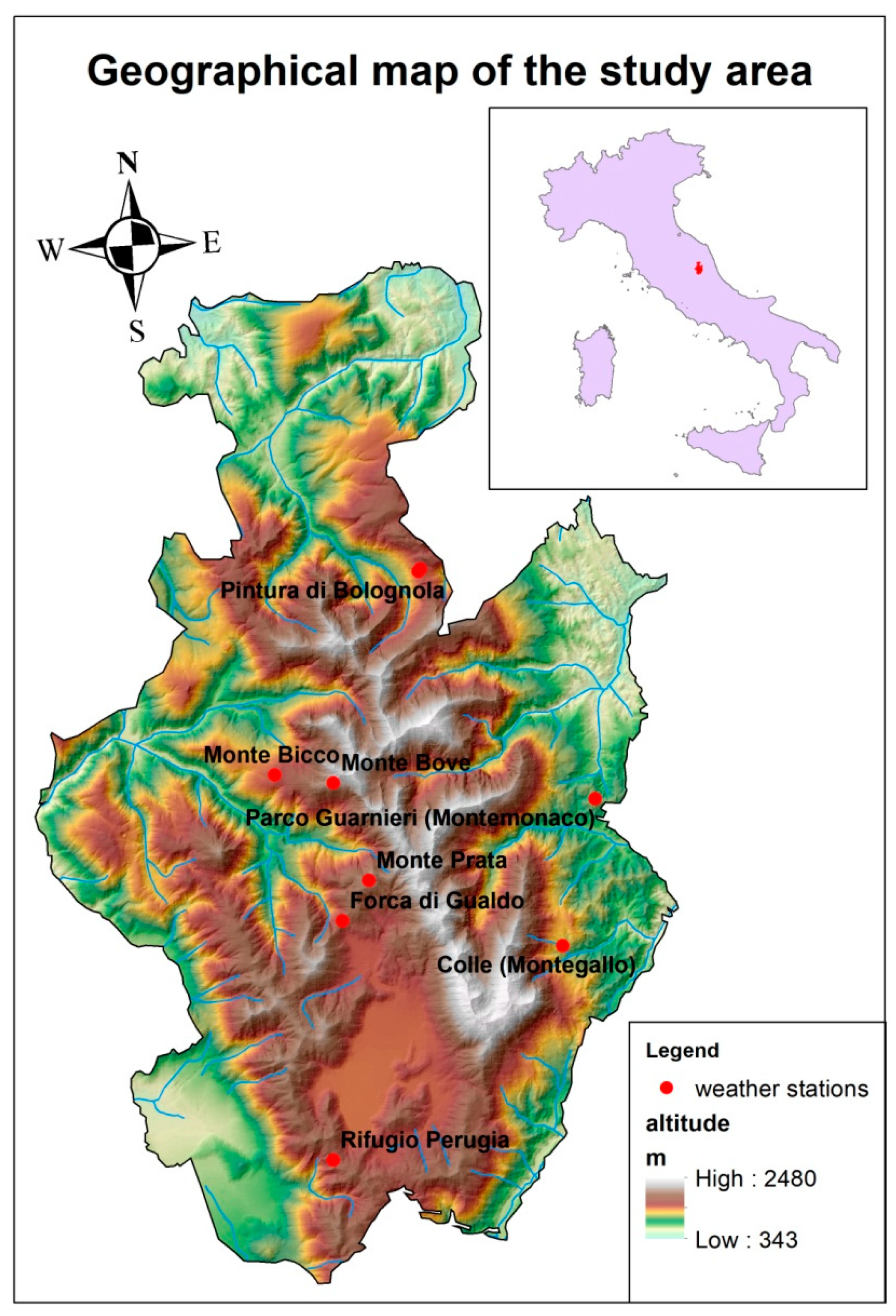
Central Italy is bordered by two seas, the Tyrrhenian Sea and the Adriatic Sea, which are the arms of the Mediterranean Sea; however, depending on their size, they influence the climate of the inland areas to a greater or lesser extent. The Monti Sibillini National Park is located between two Italian regions, Marche and Umbria, and its territory consists of sixteen municipalities belonging to four different provinces. The extent of the study area is approximately 697 km2, which includes numerous mountains above 2000 m, the highest of which is Monte Vettore at 2476 m, where the average altitude of the area is 1173 m a.s.l. (Figure 1). The park is the source of four main rivers, including the Aso, the Tenna, and the Fiastrone, which flow into the Adriatic Sea to the east, and the Nera, which flows into the Tyrrhenian Sea, as well as numerous other minor watercourses.
2. Materials and Methods
The snow cover data were collected from two different databases, that of the Functional Multiple Risk Centre of the Civil Protection of the Marche Region and that of the METEOMONT service, which are responsible for monitoring the snowpack and avalanche risk in Italy. Ten weather stations were considered for the period 2010–2022, while for the period 1991–2020, six stations were available in the area (Table 1). In particular, the 4 stations from the Functional Multiple Risk Centre (Monte Prata, Monte Bove, Pintura di Bolognola, and Sassotetto) are equipped with a sonar that measures the snow depth on the ground every 30 min, while the remaining 6 weather stations are manual weather stations, where the surveyor goes to the site and by means of a graduated rod notes the measurement once a day. With these two detection methods, the measurement errors are significantly reduced compared to other methods such as the heated rain gauge, which is exposed to wind problems, especially in mountain environments.
Data were collected for each year from the beginning of November to the end of April and were evaluated on both a monthly and annual scale. The variables of interest for the snowpack were identified in 3 main ones: days with snow cover on the ground, average snow depth, and maximum snow depth. Concerning days with snow cover on the ground, days with snow on the ground were counted for each calendar year, while for average snow depths, an average was taken for each year of all daily values, even those without snow on the ground. Finally, the maximum snow depth in the interval between November and April was isolated for each year. As far as quality control is concerned, gross error check was put into practice, as the only error that the two weather station detection systems can make is in typing, as well as the assessment of internal consistency with melt rates not exceeding the calculated threshold value per day, which can only occur if a zero is mistakenly entered in place of the missing data. Therefore, daily snowfall values of more than 250 cm and melts of more than 50 cm per day, which were assessed as statistically impossible for the study area, were eliminated, and of course, they were always verified with neighboring weather stations. Homogenization was conducted using the standard normal homogeneity test (SNHT) test; however, it resulted in null hypotheses, which is evidence that the weather stations had no perturbations that could cause inhomogeneity in the analyzed time series. In this context, it is very interesting to evaluate the possible correlation of weather stations in order to understand which areas are homogeneous and to prepare spatial procedures for validating data in the future, in cases of more uncertain detections. Therefore, the first of all the correlations between the various weather stations in the period 2010–2022 was evaluated using two methods, Pearson’s and the Kendall tau, both at an alpha significance level of 0.05. On the other hand, agglomerative hierarchical clustering (AHC) made it possible to identify preferential associations between the various mountain weather stations and was performed using the statistical software XL Stat. The AHC works with dissimilarities, and one of the products is the dendrogram, which shows the progressive grouping of data based on similarity and distance; two objects that minimize a certain agglomeration criterion when grouped together are grouped together, thus creating a class that includes these two objects, and this is conducted until the groups defined on the basis of the agglomeration criterion are defined. In this case, Kendall’s tau method was used for similarity assessment due to its robustness against possible outliers. For both the correlation calculation and the AHC, daily snow cover data were used. The weather stations from 1991 to 2020 were mainly used for trend significance analysis, evaluating them using the Mann–Kendall test. The purpose of the Mann–Kendall (MK) test is to statistically assess whether there is a monotonic upward trend, that is, the variable studied increases, or a downward trend, that is, the variable studied decreases over time. MK tests whether to reject the null hypothesis and accept the alternative hypothesis, where hypothesis H0 states that no monotonic trend is present, while in the case of hypothesis Ha there is a monotonic trend.
This tells us the difference between the measurements at time i and j, which are positive, negative, or zero.
- = previous data
- = following data
The sum of these results determines the S value and this value can be entered into the Z test.
The variance of S is calculated using the following equation:
Sen’s test assesses the true slope of a trend line only if the trend can be assumed to be linear of the following form:
- = time series of data
- and are data values at time and , respectively.
Finally, geostatistical interpolations were required to obtain a spatialization of the point data functional to a characterization of the snow cover variables identified. Given the good correlation between snow cover and altitude, the latter was chosen as the independent variable. In particular, ordinary co-kriging with altitude as an independent variable was used, as the analysis of statistical indices showed better values than methods based on geostatistical interpolation alone, without a correlated independent variable.
In this case, ordinary co-kriging (OCK) was used instead of simple co-kriging, as the assumption that the mean is known over the entire area being interpolated cannot be considered correct, due to the non-pervasive coverage of the area because of the low number of weather stations present.
- = primary variable
- = location α1
- = location α2
- = kriging weight for the α primary data sample
In order to be able to assess the goodness of an interpolative method, the cross-validation procedure with the one-leave-out method was used, which resulted in four statistical indices: mean standardized error (MSE), root mean square error standardized (RMSSE), root mean square error (RMSE), and average standard error (ASE) [24].
Root mean square error (RMSE): This is the standard deviation between observed and predicted values: t. This statistical index enables an assessment of the prediction errors for different weather stations. However, RMSE is not an absolute statistical index, since it is impossible to compare different variables with the RMSE. However, it can be useful to compare within the same data set. The value of RMSE should be the smallest possible and similar to the ASE (average standard error). In this way, when it is predicting a value at a point without observation points, it has only the ASE to assess the uncertainty of the prediction.
- = estimated value
- = observed value
- = sample size
Average standard error (ASE): This statistical tool is known to be similar to the standard deviation from the mean and is used to estimate the standard deviation of a sampling distribution. The ASE is an estimator of the bias of the RMSE (i.e., the standard deviation of the estimation error). A value close to zero and similar to RMSE represents a very low error in the estimation of the variability of the sampling distribution.
- = variance
Mean standardized error (MSE): This is similar to the mean error in that it calculates the difference between measured and predicted values; however, MSE values are not related to single variables but can be used to compare different variables. The standardization procedure leads a variable with mean of x and variance , to another with mean of zero and variance equal to 1, in order to allow comparison between different variables. The mean standardized error is represented by the ratio between the mean absolute error and the standard deviation of the estimation error.
- = standard deviation
Root mean square standardized error (RMSSE): The RMSSE enables the assessment of the goodness of the prediction models; it is desirable to have a value close to 1. If the value of RMSSE is less than 1, the variability is overestimated; otherwise, it is underestimated. This is a dimensionless statistical tool, independent from the considered variable. It is the most significant instrument to evaluate the interpolative model with other variables.
3. Results
3.1. Correlation of Snow between Different Weather Stations
In order to obtain a good snow characterization of an area, it is necessary to understand the correlation and presence of possible clusters, as the local atmospheric dynamics are greatly influenced by the topography, which inevitably shields certain air masses, creating differential snow depth even in apparently homogeneous areas. The correlation was tested using Pearson’s and Kendall’s tau methods for the period 2010–2022 for daily snow depths data on the ground, as the data are almost complete for the entire period and all weather stations analyzed are present at the same time (Table 2 and Table 3). The reason for using two methods to assess the correlation is that they provide a better characterization of the time series analyzed, as the Pearson correlation, being based on the mean, is rather sensitive to outliers.
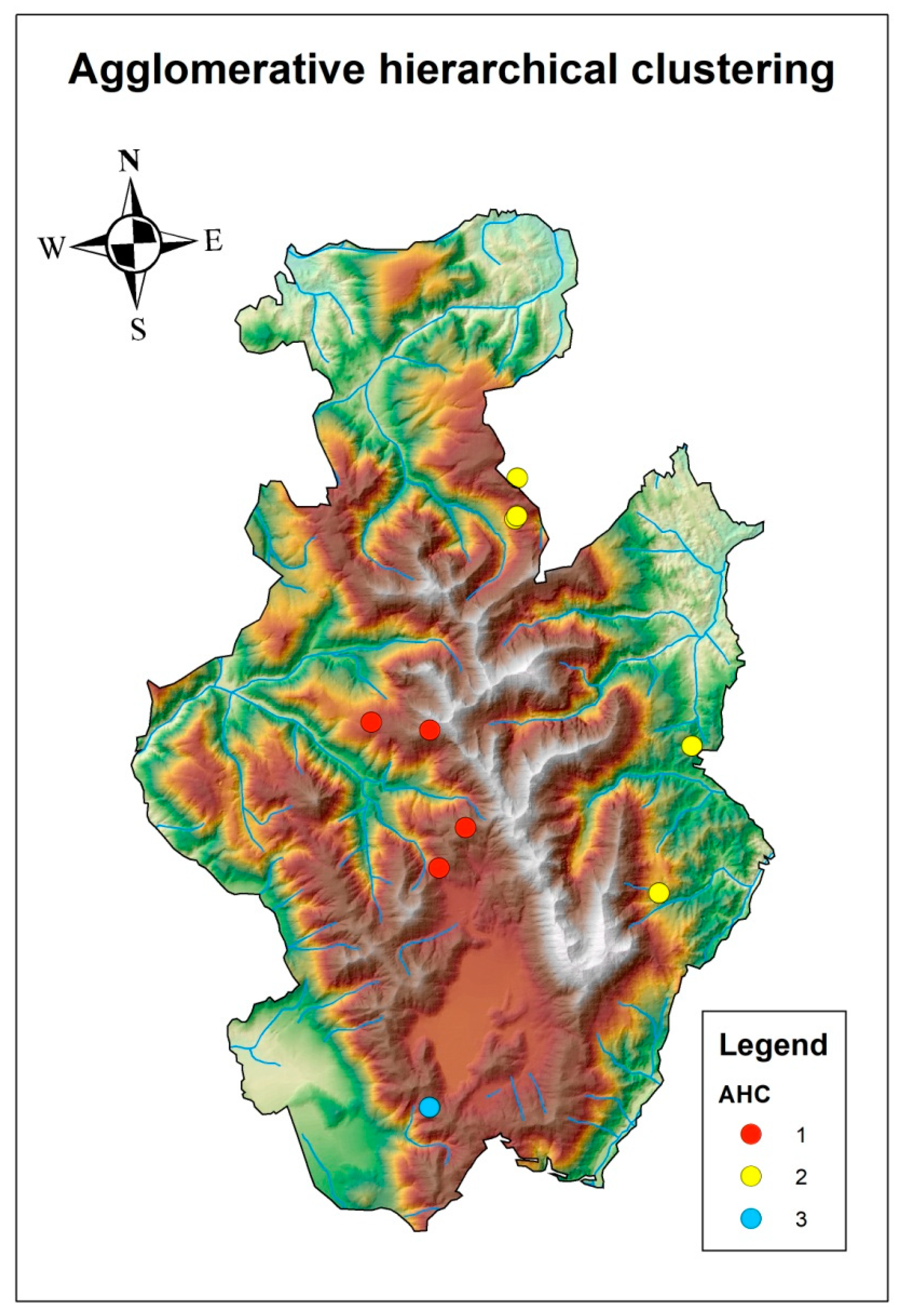
Agglomerative hierarchical clustering was crucial in order to be able to identify the associations between different weather stations regarding snow depths over the period 2010–2022. In this first analysis, it is interesting to note that only the closest weather stations are similar to each other, especially those that occupy the same slopes. This is clear evidence of the influence of topography on local atmospheric dynamics (Figure 2). Daily ground snow data were used to evaluate agglomerative hierarchical clustering in order to identify whether there may be clusters of weather stations that show similar trends in ground snow cover and consequently are exposed to the same atmospheric dynamics. The first group includes Forca di Gualdo, Monte Bicco, Monte Bove, and Monte Prata, while the second group includes Colle, La Valletta, Parco Guarnieri, Pintura di Bolognola, and Sassotetto, while Rifugio Perugia is the only weather station facing the Tyrrhenian slope in its own group (Figure 2).
3.2. Trend Test for the Period 1991–2020
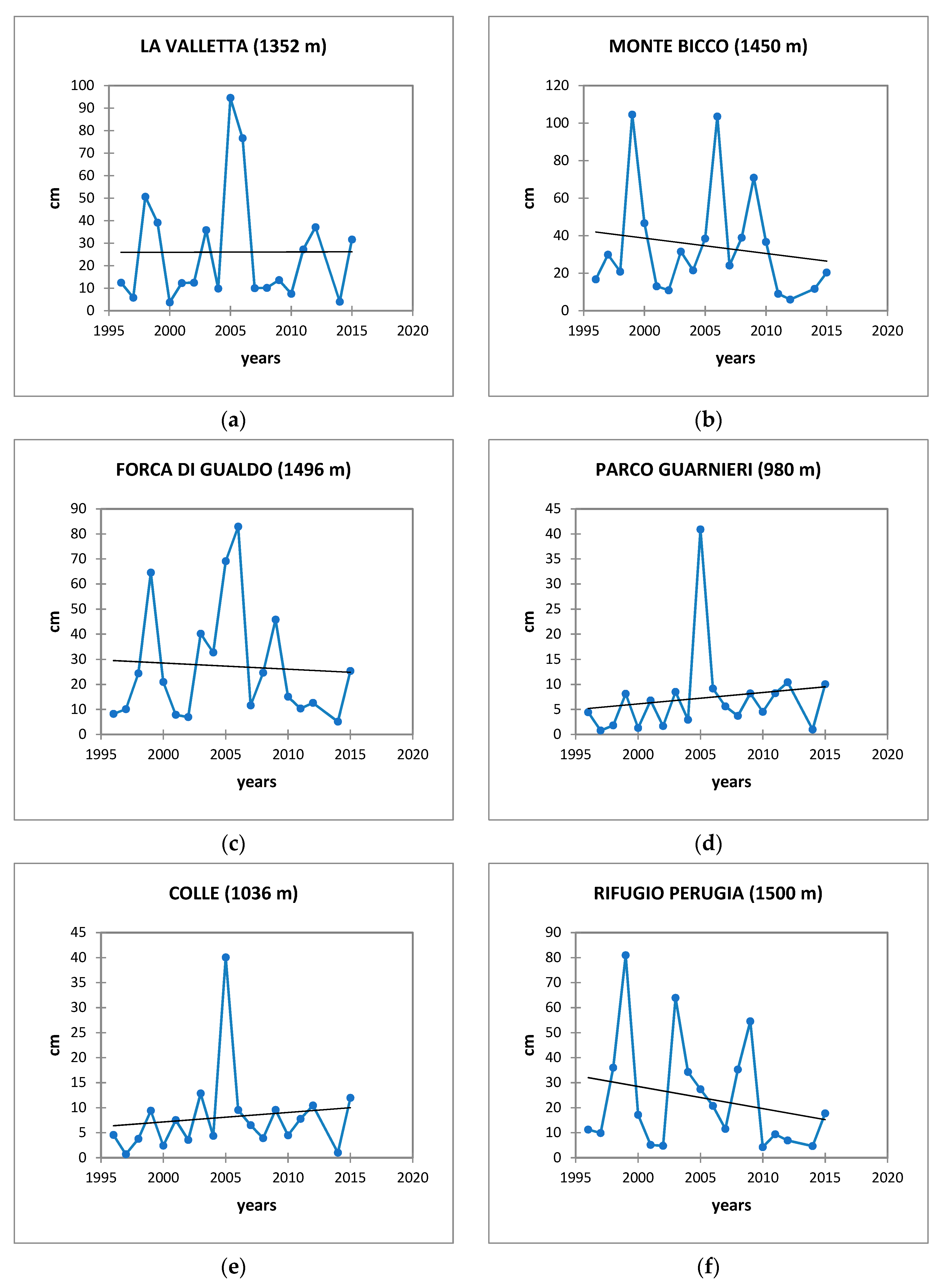
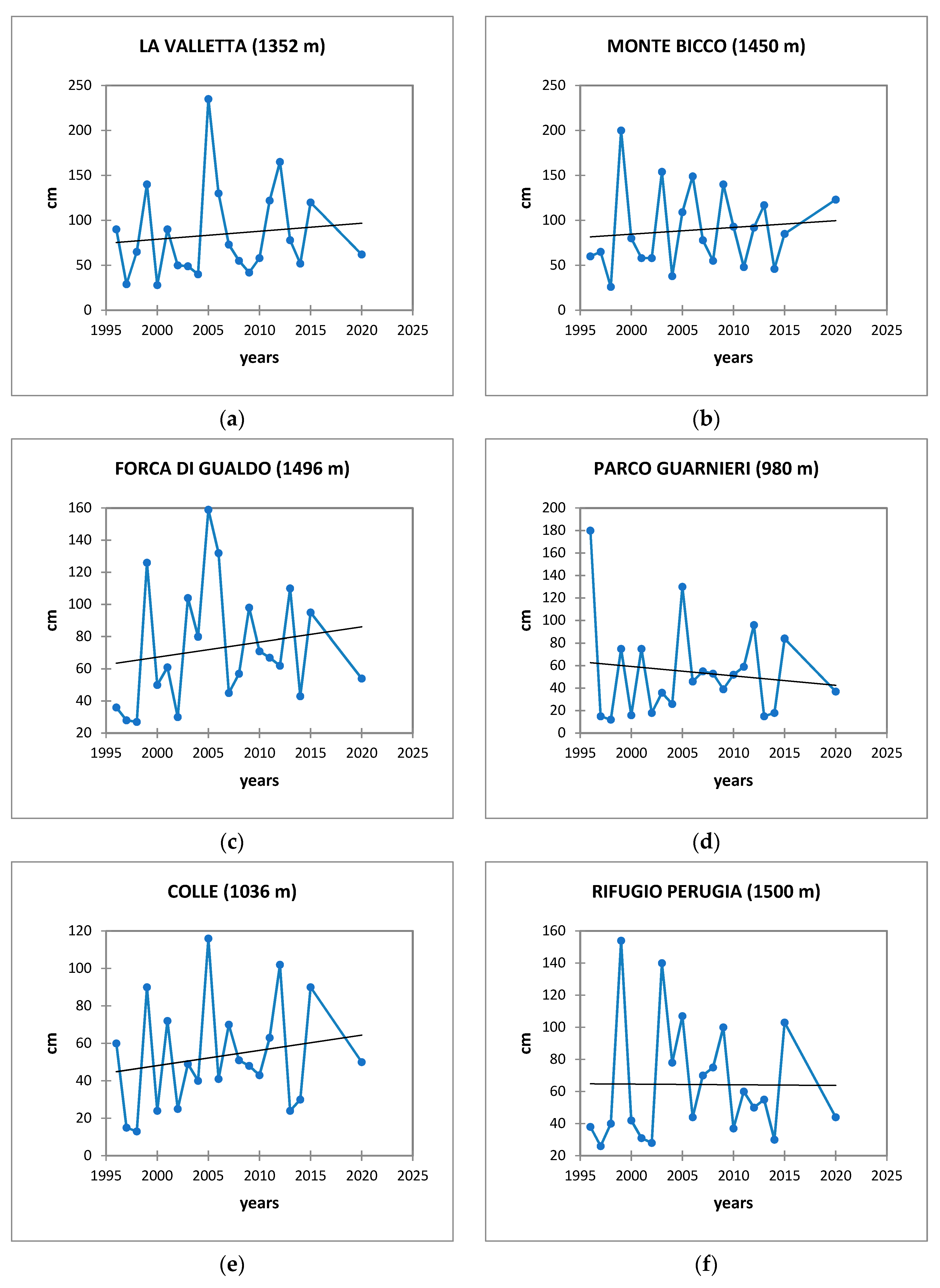
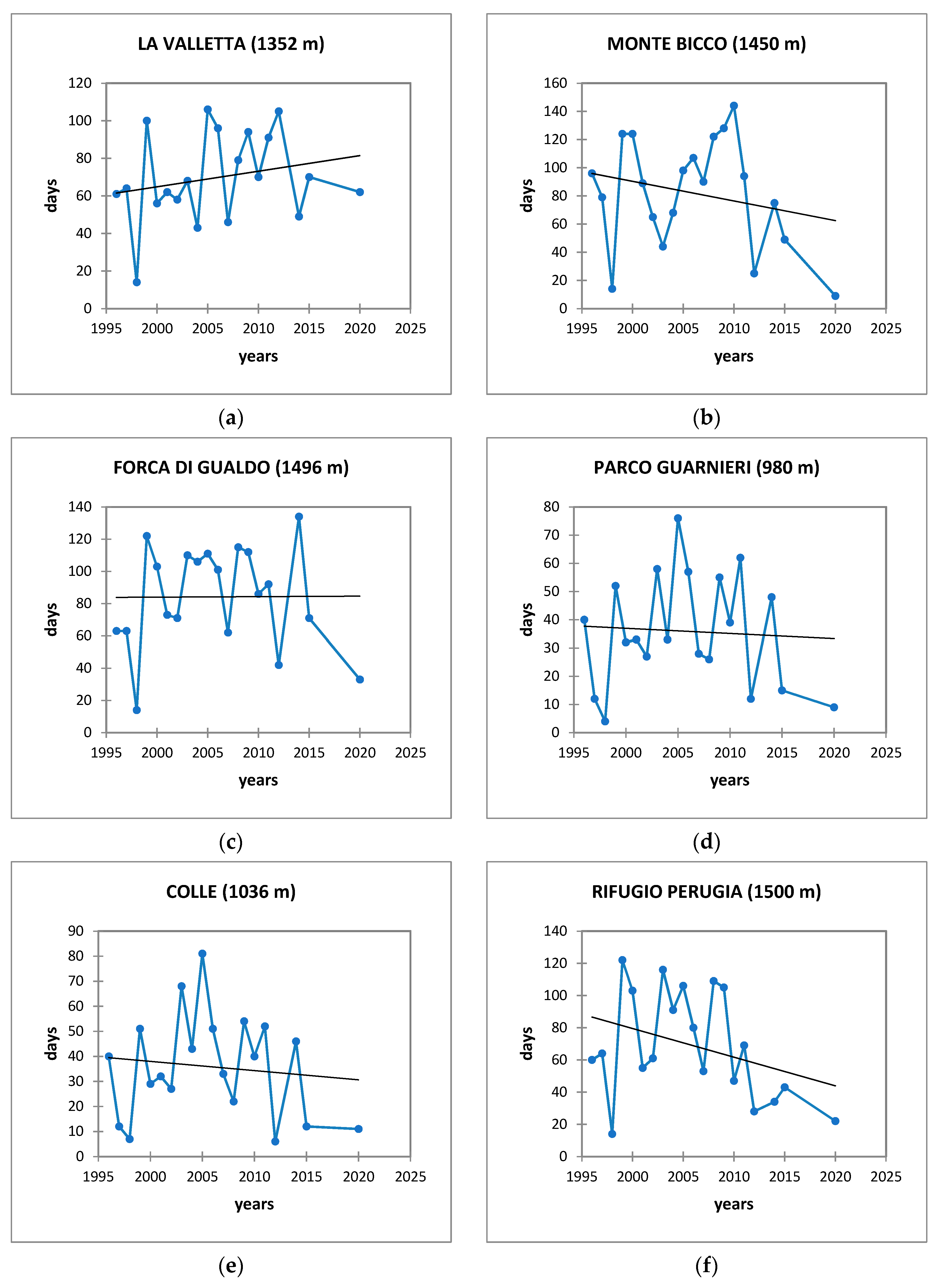
Trend analysis is the fundamental tool for answering the question of whether a climate change is taking place for the snow cover variable, in this case over the 30-year period 1991–2020, and whether it is significant. The trend analysis tests were performed over the 30-year reference period 1991–2020 in both annual and monthly steps; however, it was decided for reasons of practicality to show only the annual analysis, also because the monthly analysis has similar results. In particular, it was observed that there are no significant trends in the average snow depths, in the maximums snow depths, or in the days with persistent snow on the ground. The trend shown in the graphs is decreasing for some weather stations, while for others it is increasing, although the null hypothesis cannot be discarded, as it shows a lack of 95% significance in the trend (Figure 3, Figure 4 and Figure 5). The trend line was derived through the Sen slope estimator.
The annual average of snow on the ground in the period from 1 November to 30 April each year shows a decrease for four of the six stations, although Colle and Parco Guarnieri show an increasing trend. Colle and Parco Guarnieri are two very closely related stations that show exactly opposite trends to the other weather stations (Figure 3).
Again, the trend is not significant for any of the weather stations analyzed, but in this case we have 4 stations where the maximum annual snow depths appear to increase during the 30-year period 1991–2020 and only for 2 of them do they decrease (Figure 4).
Finally, the trend of days with snow cover on the ground decreased for all the weather stations, except for Forca di Gualdo, which saw a slight increase (Figure 5).
3.3. Interpolation of Snow Cover Variables for the Period 2010–2022
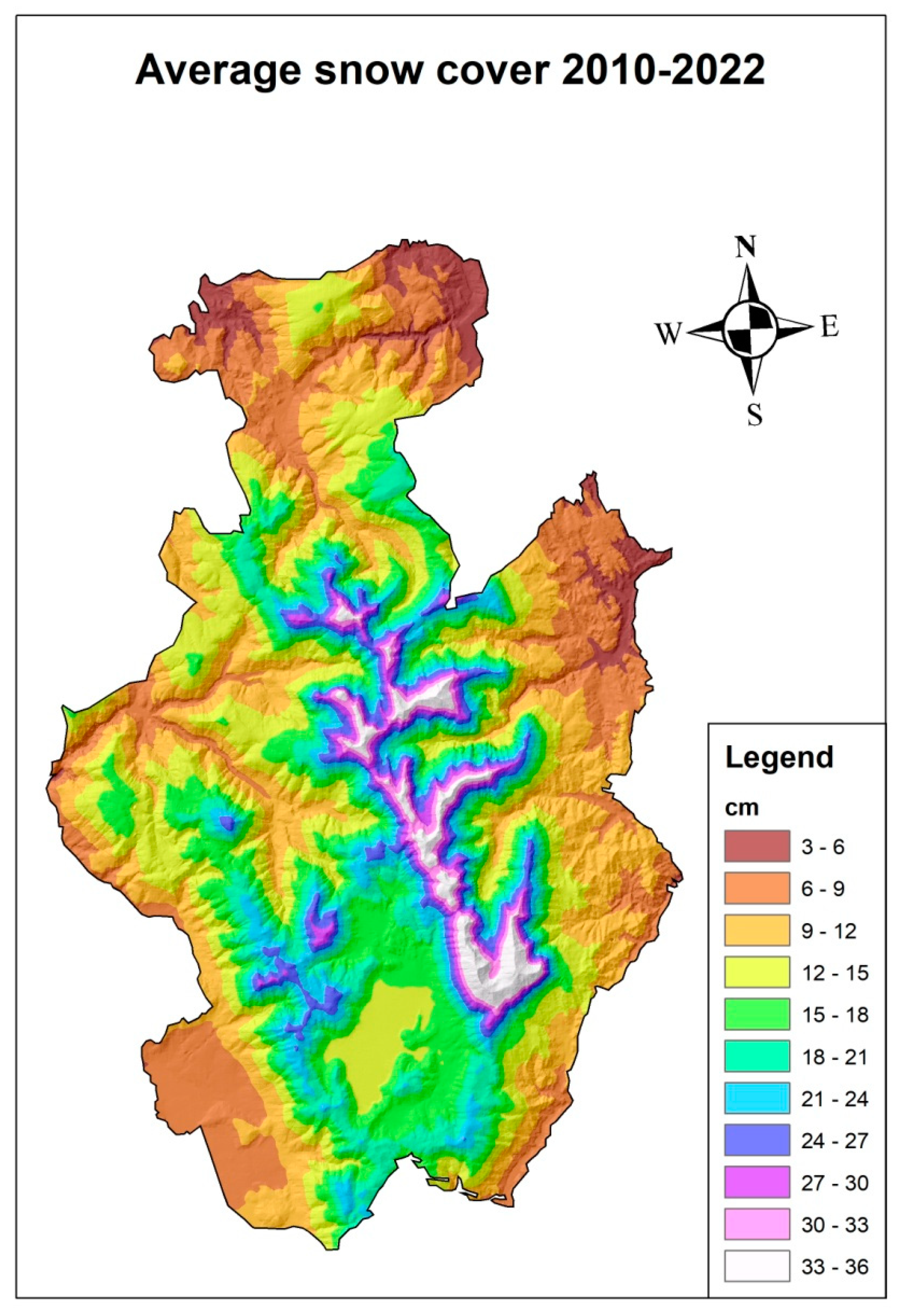
The final goal of this research is to obtain an annual mapping of the study area from 2010 to 2022 for the average snow depth, maximum snow depth, and days with snow on the ground. The interpolation of the territory of the Monti Sibillini National Park could help to quantify snowfall; however, due to the number of weather stations available, it was only possible to perform the interpolation for the period 2010–2022. Thus, data from 10 weather stations were used for the three variables of interest, and as far as the average snow cover was concerned, values from 3 cm up to 36 cm were achieved in the most surveyed parts of the territory (Figure 6).
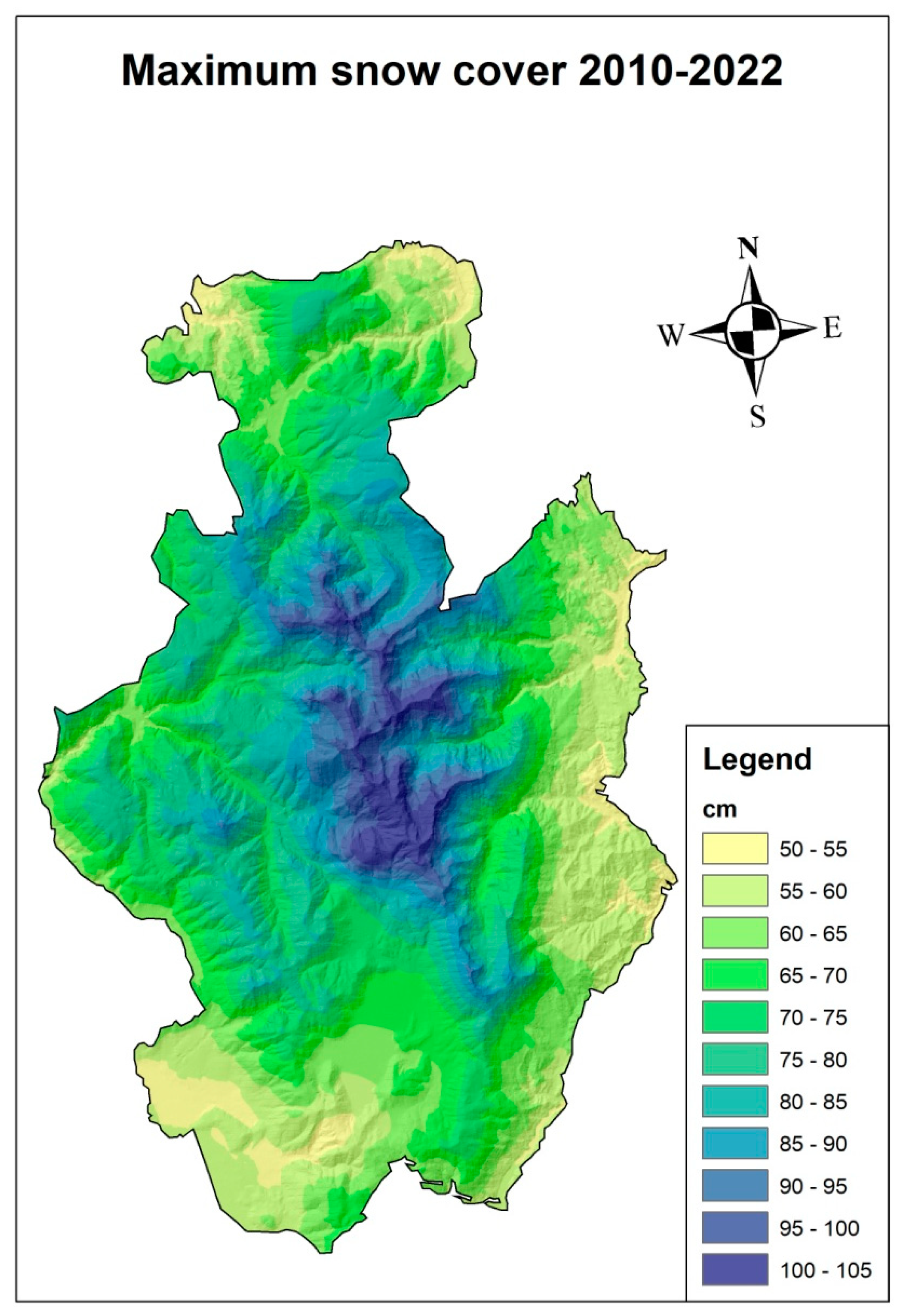
With regard to the maximum annual snow depths, the situation is very similar to that in Figure 6, although with some differences, for example in the peaks near the Colle weather station, which in this case show lower values than the peaks in the central area (Figure 7).
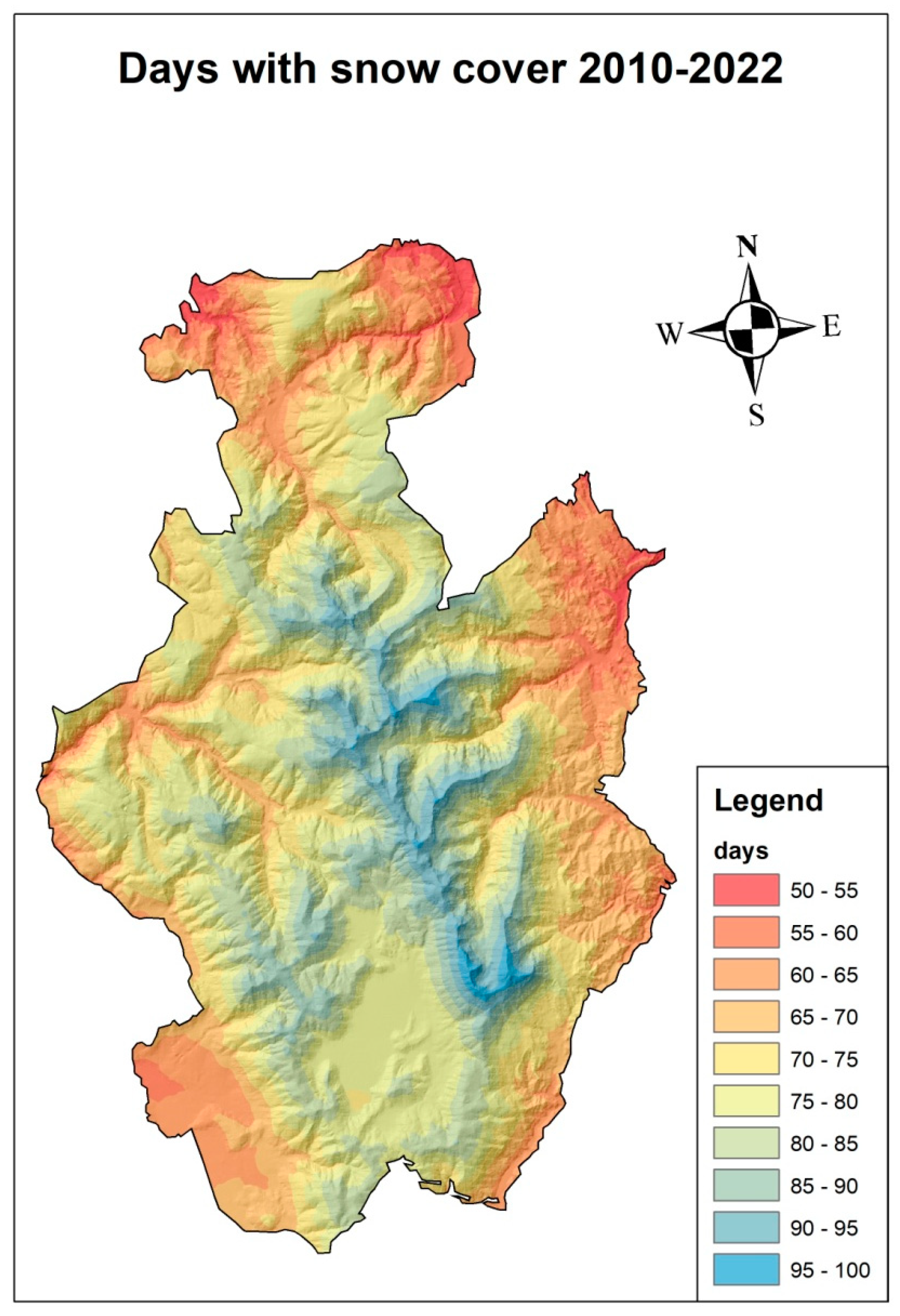
Finally, the map of days with snow cover on the ground also shows more persistent coverage in the case of the major peaks, which gradually decreases as one moves toward the hilly area (Figure 8).
The interpolations achieved a good quality, as is evident from the statistical indices calculated following cross-validation (Table 4).
4. Discussion
The aim of this research was to characterize the area of the Monti Sibillini National Park in Central Italy from the snow cover point of view, a mountainous area that has never before been analyzed in in relation to this climatic variable. The purpose of this research was two-fold: on the one hand, an analysis of the nivometric trend of the 30-year period 1991–2020 was performed, while on the other hand, a nivometric analysis was obtained with regard to the maximum and average annual snow depths, as well as an assessment of the ground persistence of snow, over the last period 2010–2022, which would provide a current and up-to-date basis for future research on afferent fields. In addition, the similarity between the available weather stations was also characterized by evaluating their correlation and applying AHC in order to understand the differences, showing weather stations that are close to each other but with different exposure to prevailing air masses. This research has a number of innovative features, including the fact that a variable such as the maximum annual snow depth was investigated, which is uncommon among research in the field but is of clear interest from the perspective of an in-depth assessment of climate change [25]. Another innovative feature of this study is that it provides a reliable interpolation of recent snow cover (2010–2022) and also allows the area to be characterized in terms of both the trends and similarities for the snow variable between the different areas of the Monti Sibillini National Park. Moreover, there were as many as three clusters in this restricted area, which was very significant, and is a symptom of a local atmospheric dynamic that is also very varied due to the position of the Apennine chain. Evaluating this result in light of other studies on much larger territories, we note much less marked dissimilarities that are practically non-existent on such limited territories [9]. In recent years, research on snow cover on the ground has turned toward satellite instruments that can cover the Earth’s surface more evenly and sometimes more accurately, due to the problems that rain gauges have in terms of counting solid precipitation in certain environments [25,26]. In this case, on the other hand, data were obtained from weather stations equipped with sonar to assess the depth of the snow and from manual weather stations, where the measurements were taken in the presence of the operator. Data from heated rain gauges were deliberately discarded because they are very often inaccurate due to the strong winds in a mountain environment, which generate significant underestimates when counting the snowpack thickness [17,27]. Moreover, in this part of the Apennines in central Italy, detailed snow cover studies had never been carried out, given the fragmentary and scarce data. The retrieval, homogenization, and validation of data was a long process, but one that allowed for an important result aimed at climate characterization using reliable weather stations, which is similar to what has been performed in other mountain environments where surveys are longer and more comprehensive [9]. In terms of the analysis, results have been reached that are in line with, but also differ from, the scientific literature on the subject. For example, a trend analysis revealed a slight decreasing trend and only for some weather stations from 1991 to 2020, an occurrence that is also refuted by other research, since a definite decrease in snowfall is considered to have occurred in the 1990s [28,29,30]. Unfortunately, in this case, it was not possible to assess the trends prior to the 1990s, due to a lack of reliable nivometric data. Finally, interpolation using GIS software with geostatistical techniques is the final result of this research; however, it is quite rare, especially in relation to the scarce availability of the complete snow data, to conduct a spatial analysis of the ground snow cover data. The use of the altitude-based co-kriging technique is most common for temperature and precipitation; however, there are also cases in the literature where it has also been used for snow cover [31,32]. Furthermore, it is necessary to specify that in some other pieces of research that are similar to this study, a strong dependence on the amount of snow cover on altitude could be observed [33]. Finally, it should be highlighted that the excellent correlation result found through geostatistical analysis, as the values of the statistical indices obtained are very close to the optimal values, especially when analyzing the values of the standardized statistical indices, is uncommon when it comes to interpolations for snow cover analysis [34,35]. This recent mapping of the territory makes it possible to make this tool an operational tool for many other environmental analyses, including mappings that are by no means common in the scientific literature on the subject.
5. Conclusions
Snow characterization is very important for improving the hydrological modeling of the area, as snow has a great influence on the recharge of the water table, so being able to model with reliable values is certainly preferable to reconstructing them empirically. Furthermore, understanding whether there are appreciable differences in the various months is equally important in order to assess any consequences that may be suffered by the indigenous vegetation. This research obtained clear results, such as the presence of a weak decreasing trend in daily snow cover between November and April from 1991 to 2020, which, however, is not significant. In addition, it is possible to identify the presence of at least three clusters in the study area, a sign that the local atmospheric dynamics are decisively influenced by the position of the main reliefs. Finally, this study enabled a spatial mapping of the territory, both in terms of the average and maximum annual snow cover and in terms of the days with snow cover on the ground. However, this research also has limitations, such as the number of years available for these weather stations, as only a few have data from before 1990, which would be important for a trend assessment over a longer period. In particular, it would be interesting to evaluate the data from this area backwards with those from the Alps or other Apennine areas, although extensive reconstructions would have to be carried out, which is why a prior correlation analysis and evaluation of clusters was also carried out. Finally, this analysis should be considered a starting point to supplement other available data or to correctly calibrate the available satellite products for ground snow cover in the study area.
Author Contributions
Conceptualization. M.G., A.C. and G.P.; methodology. M.G., T.P., S.M. and Y.H.; software. M.G. and R.M.; validation. M.G. and G.P.; formal analysis. M.G.; investigation. G.P.; resources. M.G.; data curation. G.P.; writing—original draft preparation. M.G.; writing—review and editing. G.P.; visualization. M.G.; supervision. A.C. and G.P.; project administration. M.G. All authors have read and agreed to the published version of the manuscript.
Funding
This research received no external funding.
Data Availability Statement
Not applicable.
Conflicts of Interest
The authors declare no conflict of interest.
References
- Drescher, M.; Thomas, S.C. Snow cover manipulations alter survival of early life stages of cold-temperate tree species. Oikos 2013, 122, 541–554. [Google Scholar] [CrossRef]
- Milbau, A.; Graae, B.J.; Shevtsova, A.; Nijs, I. Effects of a warmer climate on seed germination in the subarctic. Ann. Bot. 2009, 104, 287–296. [Google Scholar] [CrossRef] [Green Version]
- Gentilucci, M.; Barbieri, M.; Burt, P. Climate and territorial suitability for the Vineyards developed using GIS techniques. In Exploring the Nexus of Geoecology, Geography, Geoarcheology and Geotourism: Advances and Applications for Sustainable Development in Environmental Sciences and Agroforestry Research, Proceedings of the 1st Springer Conference of the Arabian Journal of Geosciences (CAJG-1), Hammamet, Tunisia, 12–15 November 2018; Springer International Publishing: Cham, Switzerland, 2018; pp. 11–13. [Google Scholar]
- Dong, C. Remote sensing, hydrological modeling and in situ observations in snow cover research: A review. J. Hydrol. 2018, 561, 573–583. [Google Scholar] [CrossRef]
- Dressler, K.A.; Leavesley, G.H.; Bales, R.C.; Fassnacht, S.R. Evaluation of gridded snow water equivalent and satellite snow cover products for mountain basins in a hydrologic model. Hydrol. Process. 2006, 20, 673–688. [Google Scholar] [CrossRef]
- Matsuura, S.; Okamoto, T.; Asano, S.; Osawa, H.; Shibasaki, T. Influences of the snow cover on landslide displacement in winter period: A case study in a heavy snowfall area of Japan. Environ. Earth Sci. 2017, 76, 362. [Google Scholar] [CrossRef]
- Gentilucci, M.; Barbieri, M.; Dalei, N.N.; Gentilucci, E. Management and Creation of a New Tourist Route in the National Park of the Sibillini Mountains using GIS Software, for Economic Development. In Proceedings of the 5th International Conference on Geographical Information Systems Theory, Applications and Management, Crete, Greece, 3–5 May 2019; pp. 183–188. [Google Scholar]
- Zhu, L.; Ma, G.; Zhang, Y.; Wang, J.; Tian, W.; Kan, X. Accelerated decline of snow cover in China from 1979 to 2018 observed from space. Sci. Total. Environ. 2022, 814, 152491. [Google Scholar] [CrossRef]
- Olefs, M.; Koch, R.; Schöner, W.; Marke, T. Changes in Snow Depth, Snow Cover Duration, and Potential Snowmaking Conditions in Austria, 1961–2020—A Model Based Approach. Atmosphere 2020, 11, 1330. [Google Scholar] [CrossRef]
- Martínez-Ibarra, E.; Serrano-Montes, J.; Arias-García, J. Reconstruction and analysis of 1900–2017 snowfall events on the southeast coast of Spain. Clim. Res. 2019, 78, 41–50. [Google Scholar] [CrossRef]
- Eccel, E.; Cau, P.; Ranzi, R. Data reconstruction and homogenization for reducing uncertainties in high-resolution climate analysis in Alpine regions. Theor. Appl. Clim. 2012, 110, 345–358. [Google Scholar] [CrossRef] [Green Version]
- Gentilucci, M.; Barbieri, M.; Pambianchi, G. Reliability of the IMERG product through reference rain gauges in Central Italy. Atmospheric Res. 2022, 278, 106340. [Google Scholar] [CrossRef]
- Jeoung, H.; Shi, S.; Liu, G. A Novel Approach to Validate Satellite Snowfall Retrievals by Ground-Based Point Measurements. Remote. Sens. 2022, 14, 434. [Google Scholar] [CrossRef]
- Gentilucci, M.; Pambianchi, G. Rainy Day Prediction Model with Climate Covariates Using Artificial Neural Network MLP, Pilot Area: Central Italy. Climate 2022, 10, 120. [Google Scholar] [CrossRef]
- Panahi, M.; Behrangi, A. Comparative Analysis of Snowfall Accumulation and Gauge Undercatch Correction Factors from Diverse Data Sets: In Situ, Satellite, and Reanalysis. Asia-Pacific J. Atmospheric Sci. 2020, 56, 615–628. [Google Scholar] [CrossRef]
- Tang, G.; Clark, M.P.; Papalexiou, S.M.; Ma, Z.; Hong, Y. Have satellite precipitation products improved over last two decades? A comprehensive comparison of GPM IMERG with nine satellite and reanalysis datasets. Remote Sens. Environ. 2020, 240, 111697. [Google Scholar] [CrossRef]
- Grossi, G.; Lendvai, A.; Peretti, G.; Ranzi, R. Snow Precipitation Measured by Gauges: Systematic Error Estimation and Data Series Correction in the Central Italian Alps. Water 2017, 9, 461. [Google Scholar] [CrossRef] [Green Version]
- Allamano, P.; Claps, P. Precipitation measurement errors at high-elevation sites in the Italian Alps. In Proceedings of the EGU General Assembly Conference Abstracts, Vienna, Austria, 2–7 May 2010; p. 11287. [Google Scholar]
- Pelak, N.; Sohrabi, M.; Safeeq, M.; Conklin, M. Improving snow water equivalent simulations in an alpine basin by blending precipitation gauge and snow pillow measurements. Hydrol. Process. 2023, 37, e14796. [Google Scholar] [CrossRef]
- Gascoin, S.; Lhermitte, S.; Kinnard, C.; Bortels, K.; Liston, G.E. Wind effects on snow cover in Pascua-Lama, Dry Andes of Chile. Adv. Water Resour. 2013, 55, 25–39. [Google Scholar] [CrossRef] [Green Version]
- Raparelli, E.; Tuccella, P.; Colaiuda, V.; Marzano, F.S. Snow cover prediction in the Italian central Apennines using weather forecast and land surface numerical models. Cryosphere 2023, 17, 519–538. [Google Scholar] [CrossRef]
- Tabari, H.; Marofi, S.; Abyaneh, H.Z.; Sharifi, M.R. Comparison of artificial neural network and combined models in estimating spatial distribution of snow depth and snow water equivalent in Samsami basin of Iran. Neural Comput. Appl. 2010, 19, 625–635. [Google Scholar] [CrossRef]
- Tedesco, M.; Pulliainen, J.; Takala, M.; Hallikainen, M.; Pampaloni, P. Artificial neural network-based techniques for the re-trieval of SWE and snow depth from SSM/I data. Remote Sens. Environ. 2004, 90, 76–85. [Google Scholar] [CrossRef]
- Goovaerts, P. Ordinary Cokriging Revisited. J. Int. Assoc. Math. Geol. 1998, 30, 21–42. [Google Scholar] [CrossRef] [Green Version]
- Liu, Y.; Peters-Lidard, C.D.; Kumar, S.; Foster, J.L.; Shaw, M.; Tian, Y.; Fall, G.M. Assimilating satellite-based snow depth and snow cover products for improving snow predictions in Alaska. Adv. Water Resour. 2013, 54, 208–227. [Google Scholar] [CrossRef]
- Hall, D.K.; Riggs, G.A.; Salomonson, V.V.; DiGirolamo, N.E.; Bayr, K.J. MODIS snow-cover products. Remote Sens. Environ. 2002, 83, 181–194. [Google Scholar] [CrossRef] [Green Version]
- Buisán, S.T.; Earle, M.E.; Collado, J.L.; Kochendorfer, J.; Alastrué, J.; Wolff, M.; López-Moreno, J.I. Assessment of snowfall accumulation underestimation by tipping bucket gauges in the Spanish operational network. Atmos. Meas. Tech. 2017, 10, 1079–1091. [Google Scholar] [CrossRef] [Green Version]
- Valt, M.; Cianfarra, P. Recent snow cover variability in the Italian Alps. Cold Reg. Sci. Technol. 2010, 64, 146–157. [Google Scholar] [CrossRef]
- Bulygina, O.N.; Razuvaev, V.N.; Korshunova, N.N. Changes in snow cover over Northern Eurasia in the last few decades. Environ. Res. Lett. 2009, 4, 045026. [Google Scholar] [CrossRef]
- Onuchin, A.; Kofman, G.; Zubareva, O.; Danilova, I. Using an Urban Snow Cover Composition-Based Cluster Analysis to Zone Krasnoyarsk Town (Russia) by Pollution Level. Pol. J. Environ. Stud. 2020, 29, 4257–4267. [Google Scholar] [CrossRef]
- Hong, H.P.; Ye, W. Analysis of extreme ground snow loads for Canada using snow depth records. Nat. Hazards 2014, 73, 355–371. [Google Scholar] [CrossRef]
- Gentilucci, M.; Bufalini, M.; Materazzi, M.; Barbieri, M.; Aringoli, D.; Farabollini, P.; Pambianchi, G. Calculation of Potential Evapotranspiration and Calibration of the Hargreaves Equation Using Geostatistical Methods over the Last 10 Years in Central Italy. Geosciences 2021, 11, 348. [Google Scholar] [CrossRef]
- Uno, F.; Kawase, H.; Ishizaki, N.N.; Yoshikane, T.; Hara, M.; Kimura, F.; Iyobe, T.; Kawashima, K. Analysis of Regional Difference in Altitude Dependence of Snow Depth Using High Resolve Numerical Experiments. Sola 2014, 10, 19–22. [Google Scholar] [CrossRef] [Green Version]
- Richter, K.; Atzberger, C.; Hank, T.B.; Mauser, W. Derivation of biophysical variables from Earth observation data: Validation and statistical measures. J. Appl. Remote. Sens. 2012, 6, 063557. [Google Scholar] [CrossRef]
- Harshburger, B.J.; Humes, K.S.; Walden, V.P.; Blandford, T.R.; Moore, B.C.; Dezzani, R.J. Spatial interpolation of snow water equivalency using surface observations and remotely sensed images of snow-covered area. Hydrol. Process. 2010, 24, 1285–1295. [Google Scholar] [CrossRef]
Figure 1.
Map of the study area and positioning of weather stations.

Figure 2.
Agglomerative hierarchical clustering based on daily snow depth data from 2010 to 2022.

Figure 3.
Trend of average annual snow depths from 1991 to 2020, in black the trend line, for the weather stations: (a) La Valletta, (b) Monte Bicco, (c) Forca di Gualdo, (d) Parco Guarnieri, (e) Colle, (f) Rifugio Perugia.
Figure 3.
Trend of average annual snow depths from 1991 to 2020, in black the trend line, for the weather stations: (a) La Valletta, (b) Monte Bicco, (c) Forca di Gualdo, (d) Parco Guarnieri, (e) Colle, (f) Rifugio Perugia.

Figure 4.
Trend of maximum annual snow depths from 1991 to 2020; the trend line is in black, for the weather stations: (a) La Valletta, (b) Monte Bicco, (c) Forca di Gualdo, (d) Parco Guarnieri, (e) Colle, (f) Rifugio Perugia.
Figure 4.
Trend of maximum annual snow depths from 1991 to 2020; the trend line is in black, for the weather stations: (a) La Valletta, (b) Monte Bicco, (c) Forca di Gualdo, (d) Parco Guarnieri, (e) Colle, (f) Rifugio Perugia.

Figure 5.
Trend of days with snow on the ground from 1991 to 2020; the trend line is in black, for the weather stations: (a) La Valletta, (b) Monte Bicco, (c) Forca di Gualdo, (d) Parco Guarnieri, (e) Colle, (f) Rifugio Perugia.
Figure 5.
Trend of days with snow on the ground from 1991 to 2020; the trend line is in black, for the weather stations: (a) La Valletta, (b) Monte Bicco, (c) Forca di Gualdo, (d) Parco Guarnieri, (e) Colle, (f) Rifugio Perugia.

Figure 6.
Average snow depth in the period 2010–2022 measured in cm.

Figure 7.
Maximum snow depth in the period 2010–2022 measured in cm.

Figure 8.
Days with snow cover in the period 2010–2022 measured in cm.


Table 1.
Name, name of the weather stations, Long., longitude, Lat., latitude, Alt., altitude, presence in the period 1991–2020, presence in the period 2010–2022.
Table 1.
Name, name of the weather stations, Long., longitude, Lat., latitude, Alt., altitude, presence in the period 1991–2020, presence in the period 2010–2022.
| Name | Alt. | Lon. | Lat. | 1991–2020 | 2010–2022 |
|---|---|---|---|---|---|
| Colle | 1036 | 13.30 | 42.84 | X | X |
| Forca di Gualdo | 1496 | 13.19 | 42.86 | X | X |
| La Valletta | 1352 | 13.24 | 42.99 | X | X |
| Monte Bicco | 1450 | 13.16 | 42.92 | X | X |
| Monte Bove | 1917 | 13.19 | 42.91 | X | |
| Monte Prata | 1813 | 13.21 | 42.87 | X | |
| Parco Guarnieri | 980 | 13.33 | 42.90 | X | X |
| Pintura di Bolognola | 1360 | 13.24 | 42.99 | X | |
| Rifugio Perugia | 1500 | 13.18 | 42.77 | X | X |
| Sassotetto | 1365 | 13.24 | 43.01 | X |
Table 2.
Correlation matrix performed with Pearson’s method between weather stations for daily snow depth data; the stations with a significant 95% correlation between them are in bold.
Table 2.
Correlation matrix performed with Pearson’s method between weather stations for daily snow depth data; the stations with a significant 95% correlation between them are in bold.
| Name | M. Prata | F. di Gualdo | M. Bove | M. Bicco | P. di Bolognola | La Valletta | Sassotetto | Rif. Perugia | P. Guarnieri | Colle |
|---|---|---|---|---|---|---|---|---|---|---|
| M. Prata | 1.00 | 0.53 | 0.83 | 0.80 | 0.17 | 0.00 | 0.14 | 0.55 | −0.06 | −0.05 |
| F. di Gualdo | 0.53 | 1.00 | 0.73 | 0.70 | 0.39 | 0.44 | 0.44 | 0.66 | 0.02 | 0.05 |
| M. Bove | 0.83 | 0.73 | 1.00 | 0.82 | 0.32 | 0.23 | 0.24 | 0.59 | −0.09 | −0.08 |
| M. Bicco | 0.80 | 0.70 | 0.82 | 1.00 | 0.00 | 0.01 | 0.11 | 0.24 | −0.32 | −0.34 |
| P. di Bolognola | 0.17 | 0.39 | 0.32 | 0.00 | 1.00 | 0.86 | 0.68 | 0.53 | 0.76 | 0.78 |
| La Valletta | 0.00 | 0.44 | 0.23 | 0.01 | 0.86 | 1.00 | 0.59 | 0.52 | 0.74 | 0.76 |
| Sassotetto | 0.14 | 0.44 | 0.24 | 0.11 | 0.68 | 0.59 | 1.00 | 0.26 | 0.41 | 0.45 |
| Rif. Perugia | 0.55 | 0.66 | 0.59 | 0.24 | 0.53 | 0.52 | 0.26 | 1.00 | 0.19 | 0.25 |
| P. Guarnieri | −0.06 | 0.02 | −0.09 | −0.32 | 0.76 | 0.74 | 0.41 | 0.19 | 1.00 | 0.96 |
| Colle | −0.05 | 0.05 | −0.08 | −0.34 | 0.78 | 0.76 | 0.45 | 0.25 | 0.96 | 1.00 |
Table 3.
Correlation matrix performed with Kendall’s tau method between weather stations for daily snow depth data; the stations with a significant 95% correlation between them are in bold.
Table 3.
Correlation matrix performed with Kendall’s tau method between weather stations for daily snow depth data; the stations with a significant 95% correlation between them are in bold.
| Name | M. Prata | F. di Gualdo | M. Bove | M. Bicco | P. di Bolognola | La Valletta | Sassotetto | Rif. Perugia | P. Guarnieri | Colle |
|---|---|---|---|---|---|---|---|---|---|---|
| M. Prata | 1.00 | 0.33 | 0.62 | 0.61 | 0.16 | 0.02 | 0.21 | 0.31 | 0.04 | 0.00 |
| F. di Gualdo | 0.33 | 1.00 | 0.52 | 0.51 | 0.29 | 0.38 | 0.32 | 0.41 | 0.11 | 0.12 |
| M. Bove | 0.62 | 0.52 | 1.00 | 0.63 | 0.26 | 0.19 | 0.32 | 0.34 | −0.05 | −0.05 |
| M. Bicco | 0.61 | 0.51 | 0.63 | 1.00 | 0.08 | 0.09 | 0.20 | 0.16 | −0.16 | −0.18 |
| P. di Bolognola | 0.16 | 0.29 | 0.26 | 0.08 | 1.00 | 0.64 | 0.67 | 0.35 | 0.51 | 0.55 |
| La Valletta | 0.02 | 0.38 | 0.19 | 0.09 | 0.64 | 1.00 | 0.67 | 0.36 | 0.45 | 0.50 |
| Sassotetto | 0.21 | 0.32 | 0.32 | 0.20 | 0.67 | 0.67 | 1.00 | 0.34 | 0.45 | 0.48 |
| Rif. Perugia | 0.31 | 0.41 | 0.34 | 0.16 | 0.35 | 0.36 | 0.34 | 1.00 | 0.13 | 0.20 |
| P. Guarnieri | 0.04 | 0.11 | −0.05 | −0.16 | 0.51 | 0.45 | 0.45 | 0.13 | 1.00 | 0.80 |
| Colle | 0.00 | 0.12 | −0.05 | −0.18 | 0.55 | 0.50 | 0.48 | 0.20 | 0.80 | 1.00 |
Table 4.
Statistical indices to evaluate the performance of interpolations related to the three variables under investigation.
Table 4.
Statistical indices to evaluate the performance of interpolations related to the three variables under investigation.
| Statistical Index | Average Snow Cover | Maximum Snow Cover | Days with Snow Cover on the Ground |
|---|---|---|---|
| ASE (cm) | 12.09 | 24.76 | 21.46 |
| MSE | 0.32 | 0.25 | 0.27 |
| RMSE (cm) | 8.98 | 23.17 | 21.04 |
| RMSSE | 0.85 | 0.98 | 0.98 |
Disclaimer/Publisher’s Note: The statements, opinions and data contained in all publications are solely those of the individual author(s) and contributor(s) and not of MDPI and/or the editor(s). MDPI and/or the editor(s) disclaim responsibility for any injury to people or property resulting from any ideas, methods, instructions or products referred to in the content. |
© 2023 by the authors. Licensee MDPI, Basel, Switzerland. This article is an open access article distributed under the terms and conditions of the Creative Commons Attribution (CC BY) license (https://creativecommons.org/licenses/by/4.0/).
Share and Cite
MDPI and ACS Style
Gentilucci, M.; Catorci, A.; Panichella, T.; Moscatelli, S.; Hamed, Y.; Missaoui, R.; Pambianchi, G. Analysis of Snow Cover in the Sibillini Mountains in Central Italy. Climate 2023, 11, 72. https://doi.org/10.3390/cli11030072
AMA Style
Gentilucci M, Catorci A, Panichella T, Moscatelli S, Hamed Y, Missaoui R, Pambianchi G. Analysis of Snow Cover in the Sibillini Mountains in Central Italy. Climate. 2023; 11(3):72. https://doi.org/10.3390/cli11030072
Chicago/Turabian StyleGentilucci, Matteo, Andrea Catorci, Tiziana Panichella, Sara Moscatelli, Younes Hamed, Rim Missaoui, and Gilberto Pambianchi. 2023. "Analysis of Snow Cover in the Sibillini Mountains in Central Italy" Climate 11, no. 3: 72. https://doi.org/10.3390/cli11030072
Note that from the first issue of 2016, this journal uses article numbers instead of page numbers. See further details here.