Article

Sea Level Variability in the Equatorial Malacca Strait: The Influence of Climatic–Oceanographic Factors and Its Implications for Tidal Properties in the Estuarine Zone

by
Ulung Jantama Wisha
1,2,
Yusuf Jati Wijaya
3 and
Yukiharu Hisaki
1,*
1
Physical Oceanography Laboratory, Department of Physics and Earth Sciences, Graduate School of Engineering and Science, University of the Ryukyus, Nishihara 903-0213, Japan
2
Coastal Processes Research Group, Research Center for Oceanography, National Research and Innovation Agency (BRIN), Jakarta 14430, Indonesia
3
Department of Oceanography, Faculty of Fisheries and Marine Science, Diponegoro University, Semarang 50275, Indonesia
*
Author to whom correspondence should be addressed.
Climate 2023, 11(3), 70; https://doi.org/10.3390/cli11030070
Submission received: 27 January 2023 / Revised: 8 March 2023 / Accepted: 14 March 2023 / Published: 16 March 2023

Abstract

:
The sea level trend in the equatorial Malacca Strait is a significant issue that needs to be reviewed since it is an area of interest. Assessing its future impact on estuarine tidal characteristics is worth studying because it relates to the potency of coastal damages. This study aimed to discuss the relationship between sea level variations and anomalies and their possible triggering factors and to estimate the future impacts on the tidal properties in the estuarine zone. Tide gauge and altimetry data in the Tanjong Pagar site were used to assess the sea level trends over 27 years of observation (from 1992 to 2019). Both altimetry and tide gauge data showed an upward trend, with 0.24 cm/year and 0.39 cm/year, respectively. Due to the near-equatorial area of interest, sea level variability is more synchronized with ENSO rather than IOD. At some points, ENSO shapes the sea level fluctuation, with an R2 of less than 10%. For specific periods, the coupling effects between MJO and La Niña may trigger higher evaporation in the maritime continent, triggering increasing sea levels. Of particular concern, among the other assessed factors, the zonal currents and winds (wind-driven currents) are strongly correlated with sea level variations, primarily during the NE monsoon and the second transitional periods, with a determination coefficient of about 18–36%. As a result of sea level rises, it is estimated that tidal constituent amplitudes will increase by about 8.9% and 18.3% in 2050 and 2100, respectively. The increase in tidal range will possibly relate to the tidal bore passage in the Kampar estuary. Therefore, more advanced hydrodynamic modeling is necessary to determine the impact of sea level rises on tidal bore generation.

1. Introduction

The Malacca Strait is a funnel-shaped channel between the eastern coast of Sumatra (Indonesia), Peninsular Malaysia, and Singapore; it is an area of significance for international shipping lanes, fishery resources, maritime heritages, and economic interest, connecting the Indian and Pacific Ocean [1,2]. However, recent global climate change issues have impacted the Malacca Strait region, as shown by increased sea surface temperature and level trends [3]. In terms of sea level change in the Malacca Strait, many reports demonstrating the increase trend tendency in sea level have been established, whereby based on the latest records, the rate of sea level change has reached 0.46 cm/year [4,5].
Primary causal factors that trigger the sea level rises are ocean circulation variability and climatic factors (El Niño-Southern Oscillation—ENSO; Pacific Decadal Oscillation) [4]. Several studies have reported that, at the interannual scale, sea level variability is correlated with ENSO and IOD (Indian Ocean Dipole), and its rises are correlated with La Niña and a negative IOD index [4,5]. Another study explained that sea level anomalies (SLAs) in the Malacca and Singapore Straits are significantly different and controlled by the Indian Ocean and the South China Sea [6]. On the other hand, within 27 years of observation, sea level rises in the Malacca Strait and Eastern Peninsular Malaysia ranged from 0.32 to 0.36 cm/year, significantly determined by the variability of ENSO and IOD [7]. These previous studies only compared the sea level variability with IOD/ENSO. This creates a consideration about how significantly the other climatic–oceanographic factors could trigger rising sea levels. Therefore, in addition to IOD and ENSO, the influence of ocean circulation and other climatic factors, such as Madden Julian Oscillation (MJO), on sea level variations in the equatorial Malacca Strait are worthy of assessment. Moreover, the report on sea level trends in the Malacca Strait needs to be reviewed to estimate future impacts in the surrounding coastal areas.
Concerning coastal areas, several cases of coastal damage (coastal instability and inundation) have been reported due to sea level rises. Overall, 50% of the west coast of Peninsular Malaysia is critically eroded, with a shoreline retreat of about from 1 to 100 m/year [8]. Furthermore, 40% of the Peninsular Malaysia shoreline is categorized as highly vulnerable to coastal hazards and disasters [9]. On the other hand, a study reported seawater inundation in several areas on the eastern coast of Sumatra [10]. These conditions show that the long-term impact of sea level rise would be massive on coastal regions. In addition to land subsidence tendencies, sea level changes significantly trigger coastal inundation and flooding, even changing the properties of seawater. According to [11,12], the closest impacted oceanographic parameter due to sea level change is tidal characteristics, whereby the variability of tidal constituent amplitudes and phase lag is determined by sea level as reported by [13]. Therefore, changes in tidal properties in the coastal area caused by the sea level anomaly in the equatorial Malacca Strait are crucial to study since it relates to coastal damage and instability.
Another implication is that rising sea levels could amplify the estuarine area’s tidal range [14]. As previously introduced, on the eastern coast of Sumatra, there are several significant tidal-dominated estuaries [15,16]. One of them is the Kampar estuary, which is the most extensive estuarine system in the equatorial Malacca Strait. The presence of a hydraulic jump-induced tidal bore in Kampar River reliant on the tidal range has previously been elucidated [16]. Sea level change tendencies are supposed to alter the tidal regimes in the estuary of Kampar, which has never been discussed. Therefore, this study assesses the seasonal correlation between climatic–oceanographic factors (ENSO, IOD, surface temperature, zonal currents and winds, and MJO) and the sea level variations in the equatorial Malacca Strait. As for understanding the future impacts, the influence of sea level change on tidal regimes in the Kampar estuary should also be investigated. Therefore, this study aims to review the sea level trend in the equatorial Malacca Strait, examine the most prominent factor in triggering sea level variability, and estimate the impact of sea level rises on the tidal properties in the Kampar estuary.

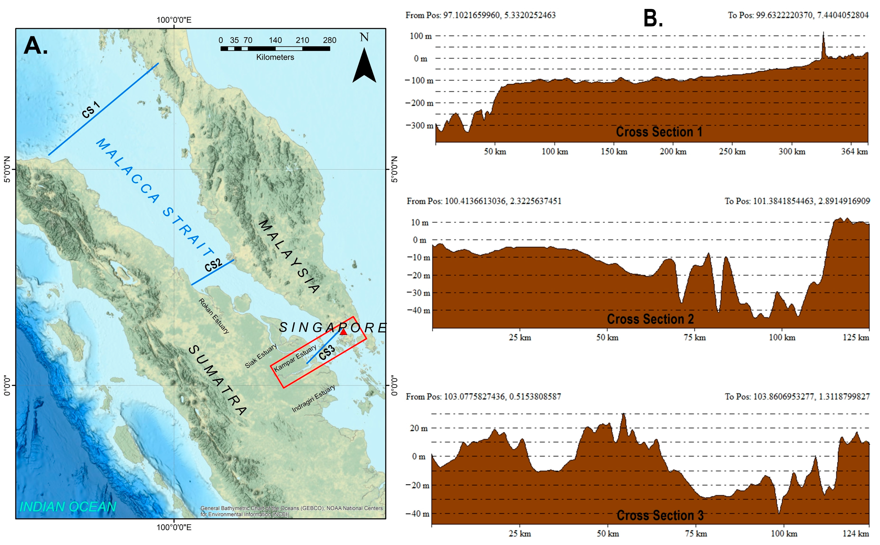
2. General Overview of the Malacca Strait

The Malacca Strait is a water channel connecting the Andaman Sea (Indian Ocean) and the South China Sea (Pacific Ocean) [1,17]. It is situated between two primary lands, the eastern coast of Sumatra (Indonesia), and the western coast of Peninsular Malaysia, with an area of about 65,000 km2. A funnel-shaped formation of the Malacca Strait lies along 800 km. The channel width is about 65 km in the south and reaches 250 km in the north [18] (Figure 1A).
The bathymetry profile in the southern part of the Malacca Strait is relatively shallow, approximately 37 m. It gradually deepens toward the northwest, reaching about 200 m, where the strait merges with the Andaman Sea [18]. Details of the bottom morphology in the southern gate, northern gate, and the middle of the Malacca Straits are shown in Figure 1B. In the northernmost area, the bottom morphology profile is steeper in the west boundary (reaching 300 m depth near Aceh Province) and becomes declivous toward the western coast of Malaysia (about 0–100 m depth). A contrary bathymetry profile is identified in the middle of the strait, where the declivous profile on the western side does exist, characterized by a less than 10 m depth and an irregular steep bathymetry in the eastern land boundary, with a depth ranging from 10 to 40 m. More arbitrarily erratic bottom morphology exists in the southern gate of the strait, ranging from 5 to 40 m. In addition to shaping the bottom morphological profiles in the shallow water area, numerous isles, some fringing reefs, and sand ridges exist within the strait, hampering the water mass flow from the southern entrance to the strait [1,17]. The sand ridge formation is induced by the material accumulation derived from large estuaries on the eastern coast of Sumatra [19].
Geologically, the Malacca Strait is part of the Sunda Shelf (an extensive, low-relief land surface from about 2.6 million years ago). It has remained undisturbed by crustal movements for the past 7 million years [20]. Another record elucidates that the current configuration of the strait is due to the inundation induced by the postglacial rise of the sea level due to the melting of land ice in higher latitude regions [21]. The coastal swamp formation characterizes both primary lands, whereby the low-slope swamp forest is arranged on the eastern coast of Sumatra with a high accumulation of sediment (sedimentation tendency) due to large estuaries [19].
The climate condition in the Malacca Strait is commonly hot and humid, characterized by the monsoon system (the northeast monsoon during winter and the southwest monsoon during summer) [1,2,3,4,5,6,7,17,18,22,23]. The average rainfall intensity ranges from 1930 to 2570 mm [17]. The sea surface temperature in the strait ranges from 28.4 to 31.1 °C [18]. The annual surface current flow is commonly directed toward the northwest (Andaman Sea) since the sea surface elevation is always higher in the South China Sea, bringing a high salinity toward the Malacca Strait during the northeast (NE) monsoon and low salinity from the Java Sea during the southwest (SW) monsoon [22]. A lower salinity is found within the strait due to the substantial discharge from large estuaries on the eastern coast of Sumatra [23].

3. Materials and Methods

3.1. Data Acquisition

To review the sea level trend in the equatorial Malacca Strait, we used the approximate 27-year sea level data (1992–2019) measured using altimetry satellites and tide gauges, provided by The Sea Level Explorer established by the University of Colorado Boulder, the University of Hawaii Sea Level Center, and NASA Jet Propulsion Lab., web page: https://ccar.colorado.edu/altimetry/ (accessed on 18 February 2022) [24]. The tide gauge data were provided by the University of Hawaii Sea Level Center (UHSLC) [25], while the altimetry data were sourced from the Propulsion Lab’s Physical Oceanography Distributed Active Archive Center (PODAAC) [26]. The tide gauge position and the sampled altimetry data are in Tanjong Pagar, Singapore, with the coordinates 103.9167° East and 1.2500° North (Figure 1).
The Dipole Mode Index (DMI) and Southern Oscillation Index (SOI) data retrieved from https://psl.noaa.gov/data (accessed on 19 February 2022) were employed to determine the states of IOD and ENSO, respectively, and to assess their influence on sea level variation in the study area. On the other hand, as we considered the influence of the zonal current on sea level, which has never been assessed to date, the Global Observed Ocean Physics 3D Quasi-Geostrophic Currents (OMEGA3D) data were used to prove the hypothesis of the zonal current’s influence in the equatorial Malacca Strait. Copernicus provides weekly data with a grid resolution of 1/4° [26], retrieved from the following webpage: https://data.marine.copernicus.eu/ (accessed on 2 December 2022). We also employed a monthly sea surface temperature (SST) and 10m u-component of the wind of ERA5 with a horizontal resolution of 0.25°. These data are provided by the Copernicus Climate Change Service (C3S), Climate Data Store (CDS) [27], retrieved from the following webpage: https://cds.climate.copernicus.eu/ (accessed on 26 January 2023).
Since the study area is around the equatorial line, the influence of MJO may be strong during the peak level of sea level anomalies over 27 years. Thus, we will address the possible effect of MJO on triggering the significant sea level anomalies in this study. The seasonally independent index to observe the MJO is the Real-time Multivariate MJO series 1 (RMM1) and 2 (RMM2), determined based on a pair of empirical orthogonal functions (EOFs) of the combination between mean near-equatorial 850-hPa zonal wind, 200-hPa zonal wind, and the satellite-derived outgoing longwave radiation (OLR) [28]. The Real-time Multivariate (RMM) index was retrieved from http://www.bom.gov.au/climate/mjo/ (accessed on 19 February 2022) [29].

3.2. Statistical Analyses

We employed a linear regression analysis in this study to assess the correlation between the sea level recorded by the tide gauge and altimetry. Moreover, the same method was also applied in assessing the influence of climatic–oceanographic factors on sea level variation in the study area. A linear regression algorithm estimates the outcome of future events by establishing a linear relationship between an independent and a dependent variable [30]. This method is a supervised learning algorithm that predicts numerical variables by simulating a mathematical relationship between variables [31]. Mathematically, the linear regression function is represented by a slant line explained by the following equation:
Y = m 0 + m 1 X + e
where
  • Y  = predicted value of the dependent variable (target) for any given value of the independent variable;
  • X  = the independent variable (the variable that we expect influencing  Y );
  • m 0  = the intercept, the predicted value of  Y  when the  X  is 0;
  • m 1  = the regression coefficient or scale factor;
  • e  = the error of the estimation.
In addition to the prediction function, the regression model employs a cost function to optimize the weights in the form of root means square error/deviation (RMSE/RMSD). RMSD is defined as the average squared difference between the observed and predicted values. The output is typically a single number that represents the cost, or score, associated with the current set of weights [32]. The RMSD value shows the accuracy of the regression model as follows:
R M S D = 1 N i = 1 n y i y 2 1 / 2
where
  • N  = total number of observations (data points);
  • y  = estimated value of a model;
  • y i  = the actual value of observation.
Another statistical analysis we used in this study along with the linear regression results is the analysis of variance (ANOVA). ANOVA is a framework that provides knowledge about the levels of variability within a regression model and serves as the foundation for tests of significance [33]. It is similar to linear regression, but one significant difference is that regression is used to predict a continuous outcome based on one or more continuous predictor variables [34].

3.3. Estimating the Sea Level Projection Impacts on Tidal Characteristics in Estuarine Zone

Concerning the impact of the sea level upward trend on the tidal characteristics in the estuarine area, we employed classic hydrodynamic modeling (applying a NAO99b and ERG models) that was previously used in the estuarine zones by the authors of [15,16]. After quantifying the tide gauge-based sea level linear trend of 0.39 cm/year over 1992–2019, the tidal model is re-simulated considering the sea level rise projection of about 12.09 cm and 31.59 cm in 2050 and 2100, respectively. In this stage, the mean sea level over 1992–2019 from tide gauge measurement is frequency-analyzed to determine the average value, which is then tabulated to the expected sea level rise [35]. It should be noted that the sea level rises future estimations are based on the actual trend for 27 years of sea level observation in the equatorial Malacca Strait. However, since we used a linear projection of the actual assessed data, different results and conditions in the future are possible.
In addition to the model’s accuracy, it was tested by comparing field-measured surface elevation data recorded in the mouth of the Kampar estuary (equatorial Malacca Strait) during April and August 2016 [16]. The root means square error (RMSE) gained from this model simulation was less than 5 cm and 30° for tidal constituent amplitudes and phase lags, respectively, meaning that the model used could represent the field condition with a slight tolerance of uncertainty value.

4. Results and Discussions

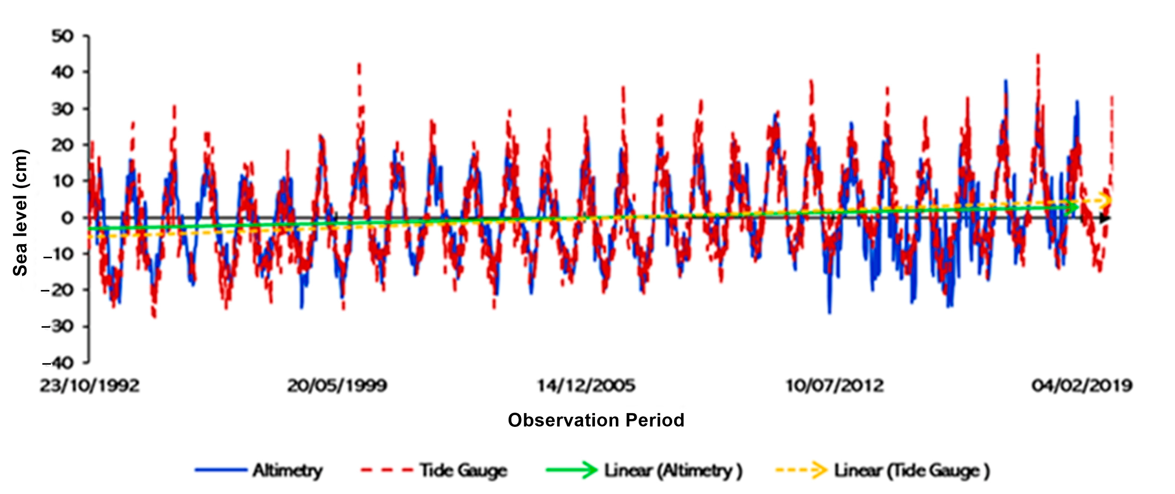
4.1. Sea Level Trends in the Equatorial Malacca Strait over 27 Years of Observation

Over 27 years, the sea level in the equatorial Malacca Strait showed an upward trend in terms of both the altimetry and tide gauge data (Figure 2). The sea level trend based on the tide gauge record was 0.39 cm/year, and the altimetry exhibited a lower trend with a deviation of about 0.15 cm/year. The overall root means square deviation (RMSD) between those data is 0.788 cm, whereby a significant noise signal extracted from altimetry was detected from 2012 to 2018. Based on the linear regression analysis, the correlation coefficient of those two compared data sources is 0.78, with an R2 of about 0.61, showing that these data are strongly correlated. Moreover, based on the analysis of variance (ANOVA) test, the examined SLA data are reliable (statistically significant) with a significance F of about less than 0.05 (5%).
Generally, the sea level measured by the tide gauge is higher than that measured with altimetry with a deviation of about 5–15 cm at certain times during the peak phase of sea level, such as in December 1993, February 1995, December 2006, December 2011, December 2013, and December 2017. The highest deviation was in December 2006, reaching 15 cm. In contrast, except for the erratic low phases during 2012–2018 (7–10 cm sea level deviation), there was no significant deviation between the tide gauge and altimetry during the low phase of sea level.
The sea level trends over 1992–2019 for altimetry and the tide gauge data were 0.24 cm/year and 0.39 cm/year, respectively. The annual amplitude detected was not too different, with a deviation of 0.5 cm. By contrast, the semi-annual amplitude detected by tide gauge measurement was 0.66 cm higher than the altimetry data (Table 1). A greater deviation in the sea level trend detected by the altimetry satellite and the tide gauge is observed by breaking down the period of the recorded data. During 1992–2009, the trend yielded by altimetry was 0.22 cm/year, and the tide gauge displayed a significant increase of 0.45 cm/year. However, the annual and semi-annual amplitudes were similar during the overall observation period, with around 13 and 2 cm, respectively.
More interestingly, from 2009 to 2019, the data demonstrated a downward trend, even though the decreased trend was not too considerable, with −0.18 and −0.03 cm/year for altimetry and the tide gauge, respectively. The annual and semi-annual amplitudes during this period were slightly different compared to the 1992–2019 and 1992–2009 periods, with a deviation of less than 1 cm. Despite the problematic comparison between altimetric and tide gauges due to the difference in the vertical reference system, many review papers have explained the efforts to validate satellite-derived sea levels with tide gauge data [36].
As stated, there is a gap between the tide gauge and altimetry in determining the sea level trend and anomaly. The other records of sea levels with different periods and methods show mixed results (Table 2). Overall, except for the eastern coast of Sumatra and the South China Sea, the sea level upward trend in the surrounding Malacca Strait is less than 0.5 cm/year. On the west coast of Peninsular Malaysia, the average sea level trend is about 0.26 cm/year [6,37]. Unlike the present study, the altimetry data show a higher trend than the tide gauge measurement, reaching 0.41 cm/year. Due to the different stations, calculation methods, and vertical reference, the gap value gained at the same area is possible [36].
In the Malacca Strait, the estimated sea level trend ranges from 0.24 to 0.36 cm/year, with an average of approximately 0.3 cm/year [4,7]. Due to the need for tide gauge measurements on the eastern coast of Sumatra, where there are no stations to date, the estimation of the sea level trend in the Malacca Strait is less represented, with only data recorded on the western coast of Peninsular Malaysia. Therefore, a long-term sea level observation is necessary on the eastern coast of Sumatra since several cases of seawater inundation in the coastal areas have been reported [38]. On the other hand, the estimation of sea level trends on the eastern coast of Sumatra has previously been established by [39], whereby, based on 21-year altimetry data, the sea level trend is sufficiently high, ranging from 0.48 to 0.56 cm/year.
Closer to the equatorial line (Singapore Strait), the sea level trend ranges from 0.12 to 0.46 cm/year. This result is on the same page as the present study, whereby the trend ranges from 0.24 to 0.39 cm/year. A downward trend detected in this present study indicates that a lower trend in sea level may occur, proven by the latest ten years of sea level records in this area, with a downward trend reaching −0.18 cm/year (Table 1). In contrast, another study detected a sufficiently higher trend in the South China Sea, with 0.55 cm/year [40]. Since the transport mechanism between the South China Sea, Indian Ocean, and Malacca Strait considerably relate to each other, we consider several climatic–oceanographic factors that potentially determine the variability in the sea level in the Malacca Strait. Moreover, it is necessary to observe the seasonal sea level variability to better depict the peak episode of sea level and its impact on the coastal area. We will address all those considerations in the following subsections.
Table 2. Reports of sea level trend in the surrounding Malacca Strait.
LocationSea Level TrendMeasurement PeriodMeasurement MethodSource
West coast of Peninsular Malaysia0.2 cm/year1993–2008Tide gauge dataAmi et al. (2012) [38]
West coast of Peninsular Malaysia0.14–0.41 cm/year1993–2008AltimetryAmi et al. (2012) [38]
West coast of Peninsular Malaysia0.29 cm/year1992–2006Tide gauge dataTay et al. (2016) [6]
Malacca Strait0.36 cm/year1986–2013Tide gauge dataLuu et al. (2015) [4]
Malacca Strait 0.24 cm/year1984–2011Tide gauge and altimetryLuu et al. (2015) [7]
Singapore Strait0.12–0.17 cm/year1975–2009Tide gauge dataTkalich et al. (2013) [5]
Singapore Strait0.19–0.46 cm/year1984–2009Tide gauge dataTkalich et al. (2013) [5]
Riau-Indonesia0.48–0.56 cm/year1993–2014AltimetryAriana et al. (2017) [40]
South China Sea0.55 cm/year1993–2009Altimetry and gravityFeng et al. (2012) [41]

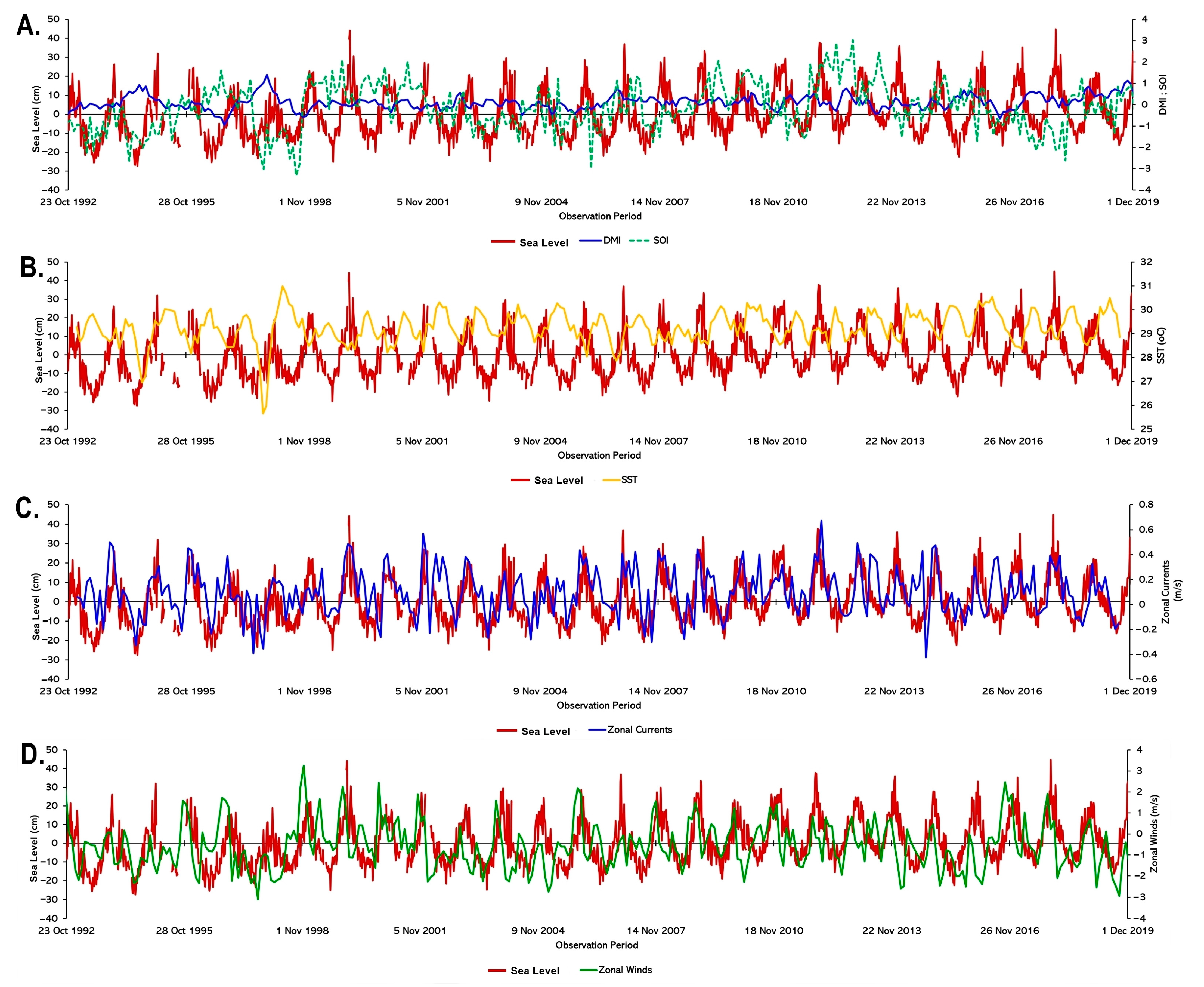
4.2. Interannual Comparison of Sea Level vs. Climatic–Oceanographic Factors

Figure 3A shows an interannual comparison between sea level and DMI-SOI. The positive mode of IOD induces higher air pressure centered in the Indian Ocean and vice versa for the negative phase of IOD, triggering the westerly wind to flow eastward and a higher sea level in the eastern Indian Ocean [41]. These mechanisms possibly impact the Malacca Strait channel via the Bay of Bengal, even though the influence is insignificant. Another study [42] stated that the ENSO-related SLA predominates in the South China Sea during specific periods. However, the influence becomes less significant at an 8-month lag time.
Due to the near-equatorial area of interest, sea level variability is more synchronized with ENSO rather than IOD. The low phase of sea level coincides with the El Niño event (prolonged period of negative SOI), such as at the end of 1992, during 1993–1994, 1997–1998, and 2017. During these periods, the SOI value reached −3, even though the fall phase of the sea level was not too significant, less than 20 cm. By contrast, La Niña episodes correlate with the high phase of sea level (denoted by the protracted positive SOI value), such as during December 1999, 2006, and 2011, where the peak phases of sea level were observed by a tide gauge in the study site, reaching 40 cm.
We also identified an opposite condition where the ENSO did not solely control the sea level state in the equatorial Malacca Strait, such as in June 1996 and December 2017 (Figure 3A). According to this state, other climatic factors, such as MJO, may trigger the SLA. In addition to the influence of IOD, several studies showed that sea level variation with IOD is commonly more substantial along the Malacca Strait channel [4,41].
Concerning sea surface temperatures (SSTs), many scholars have proven the substantial assimilation variability between SSTs and sea level variations [43,44]. However, we did not see this correlation in the equatorial Malacca Strait. Over 27 years of observation, the SSTs in the equatorial Malacca Strait ranged from 25.62 to 30.69 °C (Figure 3B). More interestingly, during the northeast monsoon of 1998, the lowest temperature reaching 26 °C was detected and peaked at 31 °C in the following period. However, after that period, the SST fluctuation seemed more uniform and stable (ranging from 29 to 30.5 °C). The SST and sea level data comparison are in the opposite modulation, tending to have an inverse response to ENSO (Figure 3B). As reported by [3], the SST in the South China Sea reaches its maximum with a 5-month lag after the mature phase of El Niño, while the sea level lowers within a 4-month phase lag. These conditions are supposed to influence SST variability in the equatorial Malacca Strait since the current flow seasonally enters the Malacca Strait via the southern channel due to a higher elevation in the South China Sea [22].
The detection of SST is commonly approached from the surface seawater temperature. On the other hand, the sea level is supposed to relate to the heat expansion of seawater in all of the ocean layers. A study revealed that SOI and seawater temperature are negatively correlated in the surface layer and vice versa below the depth of 75 m. The thermosteric sea level anomalies are strongly controlled by seawater temperature in the intermediate layer [3]. It does make sense why the modulation of surface SSTs and sea level tends to be contrary. Thus, an advanced analysis regarding the vertical variability and correlation analysis of seawater temperature and sea level is necessary for further studies.
We observed a strong modulation pattern between zonal current and sea level in the study area (Figure 3C). Of particular concern before further discussing the zonal currents, it should be noted that the positive (negative) current magnitude did not solely show the currents’ high (low) speed. However, the positive zonal currents show the predominance of eastward motion, while the negative magnitude of zonal currents shows westward movements of the water masses. These terms are also applicable to zonal wind data.
Overall, the westerly zonal current flow in the equatorial Malacca Strait coincided with increasing sea levels and vice versa for the negative zonal current profiles (flowing westward), ranging from −0.3 to 0.76 m/s. However, we identified several inconsistent patterns during the second transitional and northeast monsoon. The highest water mass transport typically occurred during the northeast monsoon as the westerly current flowed into the equatorial Malacca Strait due to the sufficiently high deviation in sea surface height [2,18,19,22]. Following these zonal currents patterns, the upward sea level phase generally coincided with eastward transport. Therefore, it seems as though the equatorial Malacca Strait becomes the accumulation center of water mass flow between the Indian Ocean via the Andaman Sea, the South China Sea, and the Java Sea, resulting in higher sea levels during the northeast monsoon [18].
Due to solid modulation patterns between zonal currents and sea levels, we considered assessing the zonal winds in the equatorial Malacca Strait. Overall, the westerly zonal winds (moving eastward) coincide with high phases of sea levels and vice versa for the easterly zonal winds (moving westward) and low phases of sea levels, even though during the peak sea levels, the zonal wind velocities were not too significant and even sometimes weaker with a magnitude of about one m/s. The strongest zonal winds were observed in November 1998, reaching 3.2 m/s, while during the other periods, commonly in the NE monsoon, the maximum velocity ranged from about 2.1 to 2.6 m/s (Figure 3D).
The sea level cross-strait in shallow water formations, such as the equatorial Malacca Strait, is considerably correlated with zonal winds [45]. The similar modulation pattern of zonal winds and zonal currents indicates that wind-driven currents significantly shape the study area’s sea level variations. Moreover, since numerous isles and estuaries characterize the study area, surface runoff plays a significant role in controlling coastal sea levels due to the influence of wind-driven circulation, as reported by [46,47]. To assess the correlation between sea level variability and climatic–oceanographic factors in the equatorial Malacca Strait, we employed a simple correlation analysis, as discussed in the following subsection.

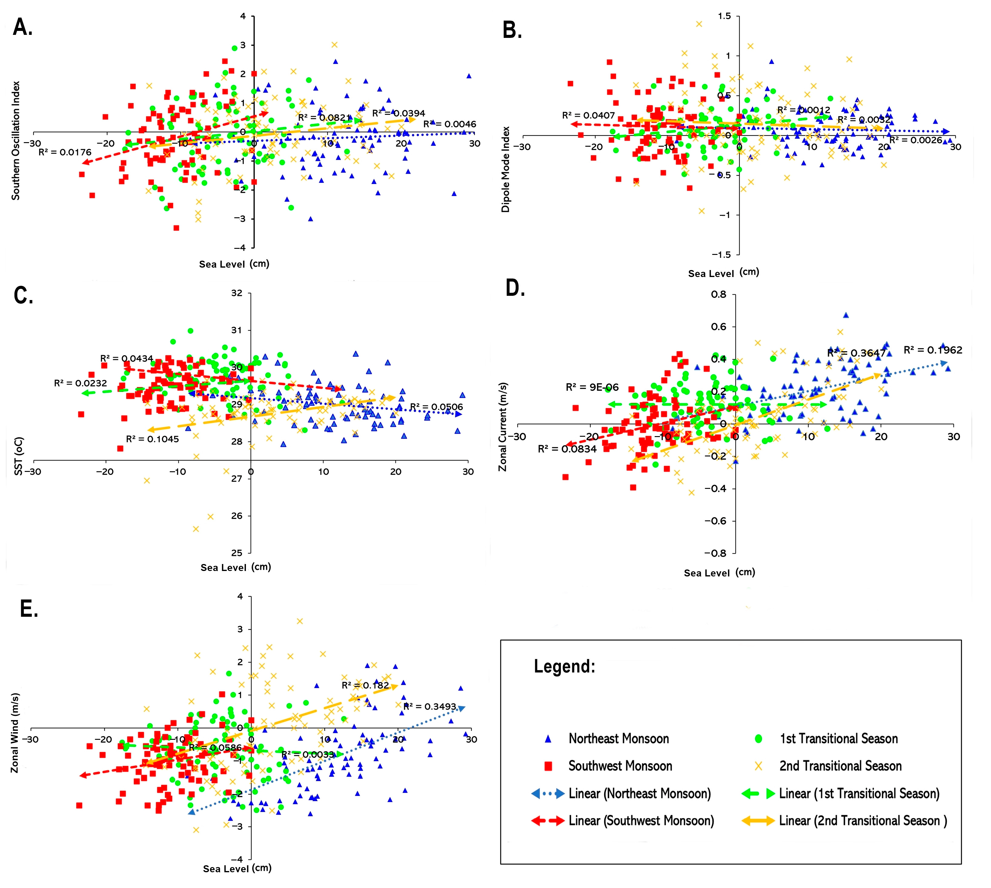
4.3. Correlation Analysis of Inter-Seasonal Variation of Sea Level vs. Climatic–Oceanographic Factors

To further assess the influence of climatic–oceanographic factors on triggering SLAs, we analyzed the inter-seasonal correlation between sea level vs. DMI, sea level vs. SOI, sea level vs. SST, sea level vs. zonal currents, and sea level vs. zonal winds (Figure 4). Overall, among all possible factors that significantly trigger sea level anomalies, zonal currents, and winds are the most correlated factors that seasonally shape the profile of sea levels in the equatorial Malacca Strait. The high phases of sea level are commonly observed during the NE monsoon and vice versa for the low phases during the SW monsoon, while during transitional seasons, the high and low phases of sea level occurred sequentially.
Concerning the correlation analysis between sea level and SOI, 8.2% of the data are correlated during the first transitional season, while the other periods showed a lower R2 value with 3.9%, 0.5%, and 1.7% for the NW monsoon, second transitional season, and SW monsoon, respectively (Figure 4A). As previously discussed, the low phases of the sea level coincide with El Niño and vice versa for the high phases of the sea level with La Niña episodes [4]. However, this state is not applicable for specific times, and at some points, during the mature phases of El Niño and La Niña, these climatic factors significantly shape the sea level profile in the equatorial Malacca Strait.
We observed a lower correlation value between the sea level vs. DMI, wherein the low phases of sea level during the SW monsoon are slightly more correlated to the Indian Ocean Dipole, with an R2 of about 4%, while for the other seasons, the correlation is relatively low, with R2 values of less than 0.5% (Figure 4B). This result indicates that the IOD did not solely control the sea level variability in the equatorial Malacca Strait. As previously mentioned, the influence of IOD is more substantial within the Malacca Strait. Therefore, the IOD control toward sea level is insignificant in the equatorial Malacca Strait (the southern gate of the strait). Otherwise, the influence of ENSO and ocean circulation from the South China Sea and Java Sea on sea level is higher in this zone.
Many studies have explained that the modulation of SST significantly reflects the sea level states [48,49]. However, in the equatorial Malacca Strait, the sea level modulation is contrary to SST fluctuation, as previously discussed. Despite that, the correlation analysis between sea level vs. STT showed more correlated data during the second transitional season, with an R2 of about 10.45% (Figure 4C), in which mainly high phases of sea level coincided with higher SSTs (ranging from 28 to 39 °C). While for the other periods, the R2 value is approximately 2.3%, 5%, and 4.3% during the first transitional season, NE, and SW monsoon, respectively.
More interestingly, despite the positive correlation between high phases of sea level and around a 20 °C SST during the second transitional season, the lowest SST over 1992–2019 (ranging from 25.8 to 27.5 °C) was also observed during the same season, coinciding with low phases of sea level. According to [50], the lower SSTs during the second transitional season relates to the seasonal southeasterly wind-driven current, transporting cooler SSTs from the South China Sea and the Java Sea, relating to the low phase of thermosteric sea levels [3].
We found that zonal-current regimes strongly correlated with sea levels during the NE monsoon and the second transitional period with an R2 of about 19–36% (Figure 4D). Moreover, the correlation value was approximately 8.3% during the SW monsoon. However, in the other transitional phases, the correlation tended to be weak (less than 0.1%), whereby the other triggering factors may influence the anomaly more in terms of sea levels, such as IOD and ENSO. To date, no studies have demonstrated the influence of zonal currents on sea levels. Thus, this finding required more advanced reviews and studies to determine the intra-seasonal and interannual correlation between them.
Concerning the zonal current profile over 27 years of observation (1992–2019), the high phase (positive) of zonal currents, primarily flowing eastward (eastern Malacca Strait), always coincided with higher phases of sea level and vice versa for the low phases of zonal currents, flowing westward and inducing lower sea level phases. According to [51], the current system in the Malacca Strait is commonly controlled by the monsoon variation and the higher sea surface height from the South China Sea, generating seasonal cyclonic and anti-cyclonic eddies, playing a significant role in southeasterly volume transport predominance, coinciding with low phases of sea level.
Similar to zonal currents vs. sea level correlation analysis, the zonal winds sufficiently control sea levels in the equatorial Malacca Strait primarily during the NE monsoon and the second transitional season with an R2 value of about 0.18–0.34% (Figure 4E). While in the other period, the zonal winds did not determine the sea level, with a determinant coefficient of less than 6%. The same pattern between zonal currents and winds in shaping the sea level fluctuations indicates that, in the equatorial Malacca Strait, a shallow water area with numerous isles on it, the influence of wind-driven currents is sufficiently substantial in controlling water motion and coastal sea levels [47].
We observed a slightly different state during the NE monsoon, whereby the high phases of the sea level (10–20 cm) coincided with the easterly zonal winds (westward winds). This state contradicts the zonal current’s influence during the same period, showing other factors controlling sea currents, such as tides, channel formation, and other kinetic energy sources [52]. This is why controls of currents and winds over sea level are probably different even though, modulation-wise, they similarly shape the sea level variability.

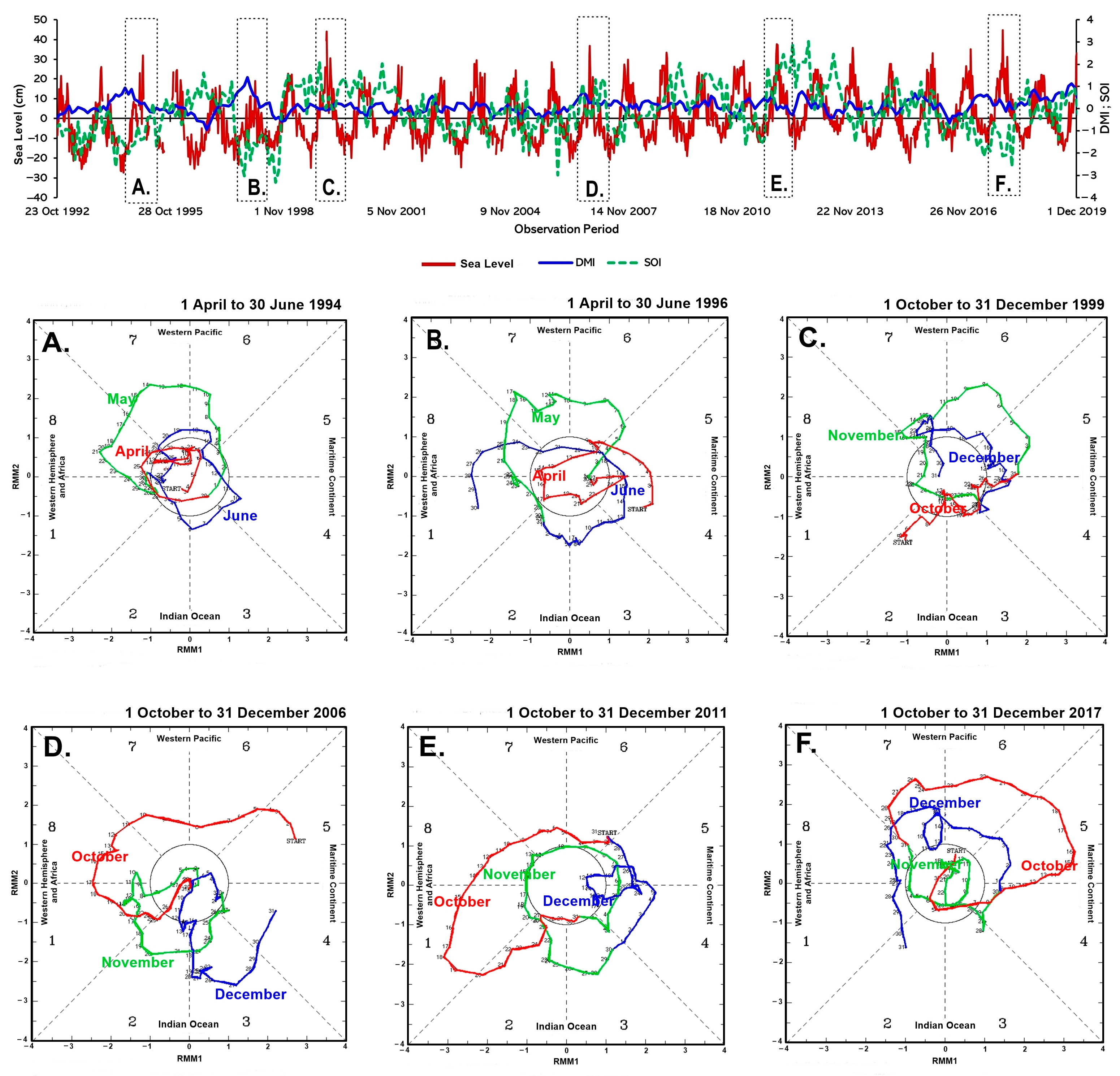
4.4. The Possible Influence of Madden Julian Oscillation (MJO) on Triggering SLA

We sampled specific periods to depict the potential influence of MJO on shaping the sea level profiles (Figure 5). The possibility of MJO determining the significant phases of sea level was sufficiently high. Except for June 1994 and June 1996 (Figure 5A,B), the strong influence of MJO on the sea level in the maritime continent (Indonesia Archipelago) during the northeast monsoon (mainly in December) was detected, shown by the positive value of RMM1 (the strong influence of MJO on triggering evaporation in the maritime continent) (Figure 5C–F) [53], affecting sea level variations in the Malacca Strait, while for June 1994 and 1996 (the southwest monsoon), the high phase of sea level is more determined by prolonged ENSO episodes and zonal transport, respectively.
Concerning April–June 1996 (Figure 5B), although the high phase of sea level was not too significant, the climatic factors also did not shape this state, shown by the prolonged El Niño (negative SOI value), low MJO influence in the maritime continent (RMM1 less than 1.5), and robust positive dipole mode (DMI > 2) (Figure 5). However, ocean circulation, such as regional wind-driven currents, shows a more substantial effect on high phases of sea level during this period (see Figure 3). This state also reflects that climatic factors have less effect on shaping sea level fluctuation. Meanwhile, ocean circulation influence is more substantial in figuring the regional sea level variations, similar to the equatorial area of the Malacca Strait.
As previously mentioned, most of the highest upward sea level fluctuations were generally identified during the NE monsoon. This state considers that MJO-induced evaporation plays a significant role in determining sea level anomalies. More substantial MJO frequencies were observed in the Indian Ocean before it finally moved toward the maritime continent of Southeast Asian countries, such as in October–November 1999, October–December 2006, and October–December 2011 (Figure 5C–E) with an RMM1 value of about 2–3.
During those periods, the highest phases of sea level coincided with prolonged La Niña events, with the positive SOI value ranging from 1 to 3. Therefore, this state possibly indicates coupling effects between MJO and La Niña, triggering higher evaporation in the maritime continent. According to [54], after inducing evaporation in the Indian Ocean region, the MJO will usually move in a clockwise direction (from west to east). MJO variability relates to warm pool generation in the eastern Indian Ocean, whereby it moves eastward as the westerly wind drifts in the equatorial line, inducing thick cumulus cloud formation and high rainfall intensity caused by warming-induced evaporation [55].
By contrast, in the middle of October 2017, when the sea level increased by about 10 cm from the previous high phase, a robust MJO frequency in the maritime continent was detected with an RMM1 value of 3.5. During the same time, prolonged El Niño episodes occurred, whereby the SOI value was negative (reaching −3) (Figure 5). This anomaly suggests that the ENSO system did not solely determine the pattern of sea levels. However, the high value of RMM1 and the increase in zonal current velocity shape the sea levels during this peak phase period.
In November 2017, the RMM index showed a weak frequency of MJO where the RMM value was within the center circle, meaning that it is arduous to discern MJO using the RMM method [56]. However, in early December 2017, the RMM index showed sufficient predomination in the maritime continent with an RMM1 value of about 1.5 (Figure 5E). Indeed, the climate processes in the equatorial Malacca Strait are multi-scale and complex [57]. Therefore, the interaction between climatic factors may have a specific influence on and affect the period of sea level anomalies, as sometimes, their control over sea level and other parameters, such as SST and chlorophyll-a, is a “seesaw” [42,58].
We tested the seasonal sea level data compared with RMM1 data using regression analysis to determine the seasonal influence of MJO on triggering sea level variability. The results show that these data are not correlated, with a correlation coefficient of less than 0.2 and an R2 (coefficient determination) of about 20% (Table 3). Of particular concern, the correlation between MJO and sea level was stronger during the NE monsoon and the second transitional season than the other periods, with an R2 of 0.022 and 0.021, respectively. This is supported by the values of standard error that are smaller during these periods, showing higher confidence in regression analysis. On the other hand, based on the ANOVA test, the value of significant F is generally more than 0.05, indicating that the variables tested are not statistically significant (unreliable).

4.5. Future Impacts of Sea Level upward Trend on Tidal Properties in the Kampar Estuary

4.5.1. Estimated Changes in Tidal Harmonic Constituents

This subsection will discuss the estimated amplitudes and phase lags changes of every dominant tidal constituent in the Kampar estuary, where the prediction is compared to a previous measurement in 2016 [16]. As previously reported, the Kampar estuary is a tidal-dominated estuary with prolonged ebb tidal currents and semidiurnal predominant co-tidal constituents [16]. Based on that, the semidiurnal (M2 and S2) constituents are expected to have a more substantial alteration due to the sea level rise impacting water-mass transfer within estuaries in the Malacca Strait [59]. However, we also consider the diurnal and shallow water tidal components (K1, O1, M4, and MS4) to determine their response to sea level rises. These are important in developing tidal characteristics in the estuary of Kampar since the mixed tide with prevailing semidiurnal characterizes it.
Table 4 shows the co-tidal amplitudes and phase lag between the tidal data measured in 2016 and the estimated data in 2050 and 2100. Overall, the tidal constituent amplitudes will increase by about 8.9% and 18.3% in 2050 and 2100, respectively. By contrast, the phase lags decrease by approximately 3.2% and 8.6% in 2050 and 2100, respectively.
As the most prominent constituents, it is estimated that the M2 and S2 amplitudes will significantly increase by, on average, 10 and 4 cm in 2050, and it will double in 2100 with the, respectively, increased elevation of 19 cm and 9 cm compared to the 2016 measured data. Since the mixed tide predominates the Kampar estuary with prevailing semidiurnal, the diurnal components are supposed to influence the surface elevation in the study area [16]. Even though the influence is insignificant, the alteration to the diurnal co-tidal component due to sea level rises should be investigated. K1 and O1 amplitudes are estimated to be slightly increased by about 4 cm in 84 years.
On the other hand, the shallow-water tides yielded from M2 and S2 interactions (M4 and MS4) exhibited a slight increase in amplitude by about 2 cm and 4 cm in 2100, respectively. These tidal constituents propagate in coastal and estuarine areas when the tidal range is no longer significant, generating new over-tide waves and even contributing to tidal asymmetries [14,60,61]. This state is supposed to play a substantial role in the hydraulic jump-off tidal bore. The increase in the amplitude of the predominant tidal constituent will impact the generation of the tidal bore in the Kampar River. However, an advanced modeling approach is necessary to precisely determine the impact of sea level rises on tidal bore in the study area.
According to [14], despite the tidal amplitude determining the tidal type, the phase lag yielded from harmonic analysis characterizes the tidal range cycle. As stated at the beginning of this subsection, the tidal phase lag value tends to decrease by about 1 to 8° over time within the influence of sea level rises. Based on the estimated value of tidal phase lag, the M2 and MS4 constituents resolve 360° more rapidly because they could complete about 170° within an hour, while the other components will be slower than that. Concerning the tidal current in the study area, even though under the scenario of sea level rises, it does not change the tidal current characteristics of the Kampar estuary, whereby it is characterized by an intense and more prolonged ebb current (ebb dominant) with the value of  2 g M 2 g M 4  ranging between −90° and 90° [16,62].

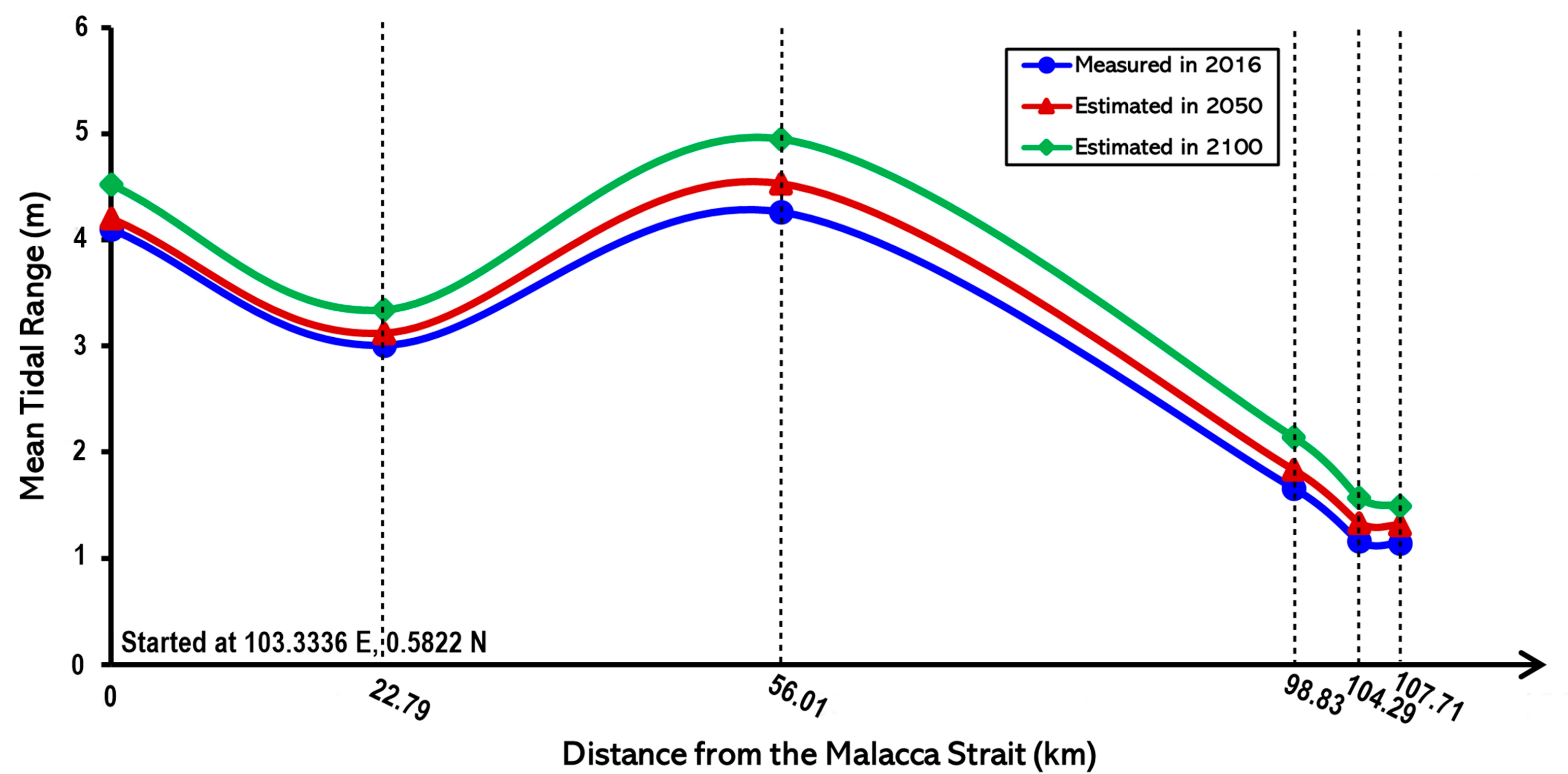
4.5.2. Sea Level Rising Trend Implication to Amplified Tidal Range in the Estuary of Kampar

By further overlooking the impact of sea level rises on the tidal range throughout the Kampar estuary, we identified tidal range amplification in the estuarine zone (about 56 km from the mouth of the estuary) (Figure 6). The estimated increase in tidal range is about 27 cm and 69 cm in 2050 and 2100, respectively. In the equatorial Malacca Strait, the tidal range amplification due to sea level rises is insignificant in 2050, with a slightly increased range, while rather significant amplification is expected to occur in 2100 with a 32 cm increase in tidal range.
At the mouth of the estuary, the tidal range is lower than in the Malacca Strait due to the sudden shallow bottom morphology, lowering the tidal amplitude [63]. The tidal range is not significantly altered by the influence of sea level increases, with approximately 20 cm. This state also applies in the upstream area where the tidal range amplitude is no longer significant. According to [16], in the upstream zone of the Kampar estuary, the tidal wave propagation (tidal bore) weakens due to the super shallow water area inducing higher bottom shear stress, hampering the water motions toward upstream, and suspended sediment deposition is predominant.
Concerning tidal range amplification in the estuarine system due to sea level rises, the result previously elucidated is consistent with the previous study identifying the considerable impact of sea level rise on the tidal range within a funnel-shaped channel, where the sea level rise generally reduces the tidal range at the mouth and changes the tidal range patterns [14,63]. As previously introduced, in the Kampar estuary, a tidal bore induced by a hydraulic jump during early flood propagation does exist, and its generation highly relies on tidal range properties in the estuarine zone. Hence, in response to sea level rises, the amplified tidal range will significantly trigger tidal bore propagation properties. This present study is only estimated based on classic hydrodynamic modeling. However, since the determination of the estuarine tidal range responses to sea level rise is complex and site-specific [14], an advanced modeling approach is necessary to understand the response of a tidal bore due to sea level rise for further studies.

5. Summary

Based on tide gauge records, an upward sea level trend was detected in the equatorial Malacca Strait over 27 years of observation (1992 to 2019), with approximately 0.39 cm/year. In contrast, a slightly declining trend was identified during the last ten years (2009 to 2019). The altimetry data also show the same pattern, even though there is a gap value between the tide gauge vs. altimetry due to the different vertical reference systems. Generally, the significant sea level difference between the tide gauge measurement and altimetry extraction is identified during the peak phases of the sea level (commonly detected during the NE monsoon), while during the low phases, there is no significant deviation from those data. Altimetry detected the erratic low phases of sea level during 2012–2018, lowering the sea level trend quantification.
Due to the near-equatorial area of interest, sea level variability is more synchronized with ENSO rather than IOD. The low phase of sea level coincides with the El Niño event (prolonged period of negative SOI), such as at the end of 1992, during 1993–1994, 1997–1998, and 2017. By contrast, the high phase of sea level generally coincided with La Niña episodes (denoted by the protracted positive SOI value), such as during December 1999, 2006, and 2011, where the peak phases of sea level are observed by a tide gauge in the study site, reaching 40 cm.
However, due to several inconsistent patterns, it is thought that ENSO did not solely control the sea level state in the equatorial Malacca Strait, such as those detected in June 1996 and December 2017. The less correlated variables between sea level vs. SOI are identified with an overall R2 of less than 10% for all periods. At some points, during the mature phases of El Niño and La Niña, these climatic factors significantly shape the sea level profile in the equatorial Malacca Strait. On the other hand, the low phases of sea level during the SW monsoon are a bit more correlated to the Indian Ocean Dipole, with an R2 of about 4%, while for the other seasons, the data are not correlated with R2 values of less than 0.5%.
The SST and sea level data comparisons are in the opposite modulation, tending to have an inverse response to the ENSO. This does make sense because SOI and seawater temperature are negatively correlated in the surface layer and vice versa for the below 75 m depth. The thermosteric sea level anomalies are strongly controlled by seawater temperature in the intermediate layer. Even though the sea level modulation is contrary to SST fluctuation, the correlation analysis between sea level vs. STT showed more correlated data, whereby over 27 years of observation, a stronger correlation is observed during the second transitional season with an R2 of about 10.45%, where mainly high-phase sea levels are correlated with higher SSTs (ranging from 28 to 39 °C), while for the other periods, the R2 value is approximately less than 5%.
On the other hand, a strong modulation pattern between zonal current and sea level is observed in the study area. Following the zonal currents patterns, the upward sea level phase generally coincided with eastward transport. Therefore, it seems as though the equatorial Malacca Straits become the accumulation center of water mass flow between the Indian Ocean via the Andaman Sea, the South China Sea, and the Java Sea, resulting in higher sea levels during the northeast monsoon. Concerning the zonal currents’ profile over 27 years of observation (1992–2019), the high phase (positive) of zonal currents, primarily flowing eastward (eastern Malacca Strait), always coincided with higher phases of SLA and vice versa for the low phases of zonal currents, flowing westward and inducing lower sea level phases. Moreover, zonal-current regimes are more correlated with sea levels during the NE monsoon and the second transitional period with an R2 of about 19–36%.
The same patterns are observed between zonal winds and SLAs, whereby over 27 years, the high phases of SLAs coincided with the positive zonal winds and vice versa for the low phases of SLAs and negative zonal winds. The strong influence of wind-driven currents in shaping local sea levels is observed since the equatorial Malacca Strait is a shallow channel with a plethora of isles and estuaries, where the controls of wind-driven currents over surface runoff evoking coastal sea levels are tremendous. Statistic-wise, the zonal winds, and SLAs are more correlated during the NE monsoon and the second transitional season than in other seasons, with a determinant coefficient ranging from 18 to 34%.
The possibility of MJO determining the significant phase of sea levels was sufficiently high. Except for June 1994, the strong influence of MJO on SLAs during the northeast monsoon (mainly in December) was detected, shown by the positive value of RMM1. More substantial MJO frequencies were observed in the Indian Ocean before it finally moved toward the maritime continent of Southeast Asian countries, such as in October–November 1999, October–December 2006, and October–December 2011, with RMM1 values of about 2–3. Due to several coincidences of prolonged La Niña and higher RMM1 values, the coupling effects between MJO and La Niña may trigger a higher evaporation in the maritime continent. Therefore, the interaction between climatic factors may have a specific influence on and affect the period of sea levels, for sometimes, their control over sea level is a “seesaw.”
Estimating the future impact of sea level rises on tidal characteristics, tidal constituent amplitudes will increase by about 8.9% and 18.3% in 2050 and 2100, respectively. By contrast, the phase lags decrease by approximately 3.2% and 8.6% in 2050 and 2100, respectively. Under the scenario of sea level rises, this does not change the tidal current characteristics of the Kampar estuary, whereby it is characterized by an intense and more prolonged ebb current (ebb dominant) with a value of  2 g M 2 g M 4  ranging between −90° and 90°. On the other hand, tidal range amplification is expected to occur in the estuarine zone (about 56 km from the mouth of the estuary), with about 27 cm and 69 cm estimated increase in tidal range in 2050 and 2100, respectively. The amplified tidal range in response to sea level rises will significantly trigger tidal bore propagation properties since it immensely relies on the tidal range.

6. Conclusions

Based on temporal tide gauge and altimetry observation (27 years), the sea level variations in the equatorial Malacca Strait showed an upward trend, even though, in the last ten years (2009–2019), slight downward trends have been observed. The sea level variability is more synchronized with ENSO than IOD, where the high phases of sea level coincided with the La Niña episodes. On the other hand, the highest phases of sea level coincided with a higher value of RMM1, indicating strong MJO frequency in the maritime continent. Even though the inter-seasonal correlation analysis between sea level and MJO (RMM1) is not significant, the coincidences of higher RMM1 values and prolonged La Niña episodes play a significant role in evoking a higher sea level variation. Among all of the possible triggering factors, zonal currents and winds showed a solid modulation to sea levels and were more correlated primarily during NE monsoon and the second transitional seasons.
It is predicted that the long-term effect of sea level rises will significantly change the tidal characteristics in the shallow water area in the equatorial Malacca Strait, thereby affecting tidal range amplification in the surrounding estuarine areas. This state may induce other coastal damage and several adaptations in the locality. Therefore, further studies assessing the impact of sea level rise in the coastal and estuarine areas in the Malacca Strait are necessary.

Author Contributions

The main contributors of this article are U.J.W. and Y.H. Conceptualization, U.J.W., Y.J.W. and Y.H.; software, U.J.W.; visualization, U.J.W.; validation, U.J.W. and Y.H.; formal analysis, U.J.W.; resources, U.J.W., Y.J.W. and Y.H.; writing—original draft preparation, U.J.W. and Y.H.; writing—review and editing, U.J.W. and Y.H.; supervision, Y.J.W. and Y.H.; funding acquisition, Y.H. All authors have read and agreed to the published version of the manuscript.

Funding

This study was financially supported by a Grant-Aid for Scientific Research (C-2) from the Ministry of Education, Culture, Sports, Science, and Technology of Japan (20K04708).

Institutional Review Board Statement

Not applicable.

Informed Consent Statement

Not applicable.

Data Availability Statement

All data used in this study appear in the submitted article and the sources are cited and referred to in the reference list.

Acknowledgments

We would like to thank University of Colorado Boulder, University of Hawaii Sea Level Center, NASA Jet Propulsion Lab., Marine Copernicus, and NOAA/OAR/ESRL PSD, Boulder, Colorado, USA for providing the primary data used in this study. Gratitude is also given to Department of Physics and Earth Sciences, University of the Ryukyus, Japan and MEXT Scholarship.

Conflicts of Interest

The authors declare no conflict of interest.

References

  1. Thia-Eng, C.; Gorre, I.R.; Ross, S.A.; Bernad, S.R.; Gervacio, B.; Ebarvia, M.C. The Malacca Straits. Mar. Pol. Bul. 2000, 41, 160–178. [Google Scholar] [CrossRef]
  2. Haditiar, Y.; Putri, M.R.; Ismail, N.; Muchlisin, Z.A.; Rizal, S. Numerical simulation of currents and volume transport in the Malacca Strait and part of south China sea. Eng. J. 2019, 23, 129–143. [Google Scholar] [CrossRef]
  3. Rong, Z.; Liu, Y.; Zong, H.; Cheng, Y. Interannual Sea Level Variability in the South China Sea and Its Response to ENSO. Glob. Planet. Chang. 2007, 55, 257–272. [Google Scholar] [CrossRef]
  4. Luu, Q.H.; Tkalich, P.; Tay, T.W. Sea Level Trend and Variability Around Peninsular Malaysia. Ocean Sci. 2015, 11, 617–628. [Google Scholar] [CrossRef] [Green Version]
  5. Tkalich, P.; Vethamony, P.; Luu, Q.-H.; Babu, M.T. Sea Level Trend and Variability in the Singapore Strait. Ocean Sci. 2013, 9, 293–300. [Google Scholar] [CrossRef] [Green Version]
  6. Tay, S.H.X.; Kurniawan, A.; Ooi, S.K.; Babovic, V. Sea level anomalies in straits of Malacca and Singapore. Appl. Ocean Res. 2016, 58, 104–117. [Google Scholar] [CrossRef]
  7. Luu, Q.H.; Tkalich, P.; Tay, T.W. Sea Level Trend and variability around the Peninsular Malaysia. Ocean Sci. Discuss. 2014, 11, 1519–1541. [Google Scholar] [CrossRef]
  8. Yanalagaran, R.; Ramli, N.I. Assessment of coastal erosion related to wind characteristics in peninsular Malaysia. J. Eng. Sci. Technol. 2018, 13, 3677–3690. [Google Scholar]
  9. Mohamad, M.F.; Lee, L.H.; Samion, M.K.H. Coastal Vulnerability Assessment towards Sustainable Management of Peninsular Malaysia Coastline. Int. J. Environ. Sci. Dev. 2014, 5, 533–538. [Google Scholar] [CrossRef] [Green Version]
  10. Lumban-Gaol, J.; Tambunan, E.; Osawa, T.; Pasaribu, B.; Nurjaya, I.W. Sea level rise impact on eastern coast of North Sumatra, Indonesia. In Proceedings of the 2nd International Forum on Sustainable Future in Asia, 2nd NIES International Forum, Bali, Indonesia, 26–28 January 2017. [Google Scholar]
  11. Khojasteh, D.; Lewis, M.; Tavakoli, S.; Farzadkhoo, M.; Felder, S.; Iglesias, G.; Glamore, W. Sea level rise will change estuarine tidal energy: A review. Renew. Sustain. Energy Rev. 2022, 156, 111855. [Google Scholar] [CrossRef]
  12. Ward, S.L.; Green, J.A.M.; Pelling, H.E. Tides, sea-level rise and tidal power extraction on the European shelf. Ocean Dyn. 2012, 62, 1153–1167. [Google Scholar] [CrossRef]
  13. Harker, A.; Green, J.M.; Schindelegger, M.; Wilmes, S.B. The impact of sea-level rise on tidal characteristics around Australia. Ocean Sci. 2019, 15, 147–159. [Google Scholar] [CrossRef] [Green Version]
  14. Khojasteh, D.; Chen, S.; Felder, S.; Heimhuber, V.; Glamore, W. Estuarine tidal range dynamics under rising sea levels. PLoS ONE 2021, 16, e0257538. [Google Scholar] [CrossRef]
  15. Wisha, U.J.; Wijaya, Y.J.; Hisaki, Y. Tidal bore generation and transport mechanism in the Rokan River Estuary, Indonesia: Hydro-oceanographic perspectives. Reg. Stud. Mar. Sci. 2022, 52, 102309. [Google Scholar] [CrossRef]
  16. Wisha, U.J.; Wijaya, Y.J.; Hisaki, Y. Real-Time Properties of Hydraulic Jump off a Tidal Bore, Its Generation and Transport Mechanisms: A Case Study of the Kampar River Estuary, Indonesia. Water 2022, 14, 2561. [Google Scholar] [CrossRef]
  17. Strait of Malacca. Available online: https://www.britannica.com/place/Strait-of-Malacca (accessed on 28 December 2022).
  18. Isa, N.S.; Akhir, M.F.; Khalil, I.; Poh, H.K.; Roseli, N.H. Seasonal Characteristics of Sea Surface Temperature and Sea Surface Currents in the Strait of Malacca and Andaman Sea. J. Sustain. Sci. Manag. 2020, 15, 66–77. [Google Scholar] [CrossRef]
  19. Iskandar, T. Modeling studies of barotropic and baroclinic dynamics in the Malacca Strait. In Proceedings of the International Conference on Science and Technology, Medan, Indonesia, 4–6 May 2018. [Google Scholar] [CrossRef]
  20. Solihuddin, T. A drowning Sunda Shelf model during last glacial maximum (LGM) and Holocene: A review. Indones. J. Geosci. 2014, 1, 99–107. [Google Scholar] [CrossRef] [Green Version]
  21. Emmel, F.J.; Curray, J.R. A submerged late Pleistocene delta and other features related to sea level changes in the Malacca Strait. Mar. Geol. 1982, 47, 197–216. [Google Scholar] [CrossRef]
  22. Rizal, S.; Damm, P.; Wahid, M.A.; Sündermann, J.; Ilhamsyah, Y.; Iskandar, T. General circulation in the malacca strait and andaman sea: A numerical model study. Am. J. Environ. Sci. 2012, 8, 479–488. [Google Scholar] [CrossRef]
  23. Ibrahim, Z.Z.; Yanagi, T. The influence of the Andaman Sea and the South China Sea on water mass in the Malacca Strait. La mer 2006, 43, 33–42. [Google Scholar]
  24. The Sea Level Explorer. Available online: https://ccar.colorado.edu/altimetry/index.html (accessed on 28 December 2022).
  25. Caldwell, P.C.; Merrfield, M.A.; Thompson, P.R. Sea level measured by tide gauges from global oceans—the Joint Archive for Sea Level holdings (NCEI Accession 0019568), Version 5.5, NOAA National Centers for Environmental Information, Dataset. Cent. Environ. Inf. Dataset 2015, 10, V5V40S47W. [Google Scholar] [CrossRef]
  26. Nardelli, B.B. A multi-year time series of observation-based 3D horizontal and vertical quasi-geostrophic global ocean currents. Earth Syst. Sci. Data 2020, 12, 1711–1723. [Google Scholar] [CrossRef]
  27. Hersbach, H.; Bell, B.; Berrisford, P.; Biavati, G.; Horányi, A.; Muñoz Sabater, J.; Nicolas, J.; Peubey, C.; Radu, R.; Rozum, I.; et al. ERA5 Monthly Averaged Data on Single Levels from 1959 to Present. Copernicus Climate Change Service (C3S) Climate Data Store (CDS) 2019. Available online: https://cds.climate.copernicus.eu/ (accessed on 25 January 2023).
  28. Wheeler, M.C.; Hendon, H.H. An all-season real-time multivariate MJO index: Development of an index for monitoring and prediction. Mon. Weather. Rev. 2004, 132, 1917–1932. [Google Scholar] [CrossRef]
  29. Madden-Julian Oscillation (MJO). Available online: http://www.bom.gov.au/climate/mjo/ (accessed on 28 December 2022).
  30. Ezer, T.; Corlett, W.B. Is sea level rise accelerating in the Chesapeake Bay? A demonstration of a novel new approach for analyzing sea level data. Geophys. Res. Lett. 2012, 39, 1–6. [Google Scholar] [CrossRef] [Green Version]
  31. Ludbrook, J. Linear regression analysis for comparing two measurers or methods of measurement: But which regression? Clin. Exp. Pharmacol. Physiol. 2010, 37, 692–699. [Google Scholar] [CrossRef]
  32. Kobayashi, K.; Salam, M.U. Comparing simulated and measured values using mean squared deviation and its components. Agron. J. 2000, 92, 345–352. [Google Scholar] [CrossRef]
  33. Campbell, H.; Lakens, D. Can we disregard the whole model? Omnibus non-inferiority testing for R2 in multi-variable linear regression and in ANOVA. Br. J. Math. Stat. Psychol. 2021, 74, 64–89. [Google Scholar] [CrossRef]
  34. Gharineiat, Z.; Deng, X. Application of the multi-adaptive regression splines to integrate sea level data from altimetry and tide gauges for monitoring extreme sea level events. Mar. Geodesy 2015, 38, 261–276. [Google Scholar] [CrossRef]
  35. Tran, K.T.; Nguyen, H.D.Q.; Truong, P.T.; Phung, D.T.M.; Nguyen, B.T. Evaluation of sea-level rise influence on tidal characteristics using a numerical model approach: A case study of a southern city coastal area in Vietnam. Model. Earth Syst. Environ. 2022, 9, 1089–1102. [Google Scholar] [CrossRef]
  36. Fenoglio-Marc, L.; Schöne, T.; Illigner, J.; Becker, M.; Manurung, P.; Khafid. Sea level change and vertical motion from satellite altimetry, tide gauges and GPS in the Indonesian region. Mar. Geodesy 2012, 35, 137–150. [Google Scholar] [CrossRef]
  37. Pajak, K.; Kowalczyk, K. A comparison of seasonal variations of sea level in the southern Baltic Sea from altimetry and tide gauge data. Adv. Space Res. 2019, 63, 1768–1780. [Google Scholar] [CrossRef]
  38. Ami, H.M.D.; Kamaludin, M.O.; Marc, N.; Sahrum, S. Long-term Sea level change in the Malaysian seas from multi-mission altimetry data. Int. J. Phys. Sci. 2012, 7, 1694–1712. [Google Scholar] [CrossRef] [Green Version]
  39. BPBD Riau Ungkap Daerah-Daerah Ini Rawan Banjir ROB. Available online: https://www.cakaplah.com/artikel/serantau/10618/2022/09/14/bpbd-riau-ungkap-daerahdaerah-ini-rawan-banjir-rob#sthash.nqeO0JDT.dpbs. (accessed on 16 January 2023). (In Indonesian).
  40. Ariana, D.; Kusmana, C.; Setiawan, Y. Study of Sea Level Rise Using Satellite Altimetry Data in the Sea of Dumai, Riau, Indonesia. Geoplanning J. Geomat. Plan. 2017, 4, 75–82. [Google Scholar] [CrossRef] [Green Version]
  41. Feng, W.; Zhong, M.; Xu, H. Sea level variations in the South China Sea inferred from satellite gravity, altimetry, and oceanographic data. Sci. China Earth Sci. 2012, 55, 1696–1701. [Google Scholar] [CrossRef]
  42. Rahmawan, G.A.; Wisha, U.J. Tendency for Climate-Variability-Driven Rise in Sea Level Detected in the Altimeter Era in the Marine Waters of Aceh, Indonesia. Int. J. Remote Sens. Earth Sci. 2019, 16, 165–178. [Google Scholar] [CrossRef]
  43. Liu, Q.; Feng, M.; Wang, D. ENSO-induced interannual variability in the southeastern South China Sea. J. Oceanogr. 2011, 67, 127–133. [Google Scholar] [CrossRef]
  44. Athie, G.; Marin, F. Cross-equatorial structure and temporal modulation of intraseasonal variability at the surface of the Tropical Atlantic Ocean. J. Geophys. Res. Ocean. 2008, 113, 1–17. [Google Scholar] [CrossRef] [Green Version]
  45. Dogan, M.; Cigizoglu, H.K.; Şanlı, D.U.; Ulke, A. Investigation of sea level anomalies related with NAO along the west coasts of Turkey and their consistency with sea surface temperature trends. Theor. Appl. Clim. 2015, 121, 349–358. [Google Scholar] [CrossRef]
  46. Vignudelli, S.; Birol, F.; Benveniste, J.; Fu, L.-L.; Picot, N.; Raynal, M.; Roinard, H. Satellite altimetry measurements of sea level in the coastal zone. Surv. Geophys. 2019, 40, 1319–1349. [Google Scholar] [CrossRef]
  47. Durand, F.; Piecuch, C.G.; Becker, M.; Papa, F.; Raju, S.V.; Khan, J.U.; Ponte, R.M. Impact of continental freshwater runoff on coastal sea level. Surv. Geophys. 2019, 40, 1437–1466. [Google Scholar] [CrossRef] [Green Version]
  48. Singh, O.P.; Khan, T.M.A.; Aktar, F.; Sarker, M.A. Recent sea level and sea surface temperature changes along the Maldives coast. Mar. Geod. 2001, 24, 209–218. [Google Scholar] [CrossRef]
  49. Singh, O.P. Cause-effect relationships between sea surface temperature, precipitation and sea level along the Bangladesh coast. Theor. Appl. Clim. 2001, 68, 233–243. [Google Scholar] [CrossRef]
  50. Nababan, B.; Rosyadi, N.; Manurung, D.; Natih, N.M.; Hakim, R. The seasonal variability of sea surface temperature and chlorophyll-a concentration in the south of Makassar Strait. Procedia Environ. Sci. 2016, 33, 583–599. [Google Scholar] [CrossRef] [Green Version]
  51. Wibowo, M.A.; Tanjung, A.; Yoswaty, D.; Susanti, R.; Muttaqin, A.S.; Fajary, F.R.; Anwika, Y.M. Understanding the Mechanism of Currents through the Malacca Strait Study Case 2020–2022: Mean state, Seasonal and Monthly Variation. In Proceedings of the 11th International and National Seminar on Fisheries and Marine Science, Pekanbaru, Indonesia, 14–15 September 2022; IOP Conference Series: Earth and Environmental Science. IOP Publishing: Bristol, UK; Volume 1118, p. 012069. [Google Scholar] [CrossRef]
  52. Wisha, U.J.; Gemilang, W.A.; Wijaya, Y.J.; Purwanto, A.D. Model-based estimation of plastic debris accumulation in Banten Bay, Indonesia, using particle tracking—Flow model hydrodynamics approach. Ocean Coast. Manag. 2022, 217, 106009. [Google Scholar] [CrossRef]
  53. Virts, K.S.; Wallace, J.M.; Hutchins, M.L.; Holzworth, R.H. Diurnal lightning variability over the Maritime Continent: Impact of low-level winds, cloudiness, and the MJO. J. Atmos. Sci. 2013, 70, 3128–3146. [Google Scholar] [CrossRef]
  54. Moum, J.N.; Pujiana, K.; Lien, R.-C.; Smyth, W.D. Ocean feedback to pulses of the Madden–Julian Oscillation in the equatorial Indian Ocean. Nat. Commun. 2016, 7, 13203. [Google Scholar] [CrossRef] [Green Version]
  55. Roxy, M.K.; Dasgupta, P.; McPhaden, M.J.; Suematsu, T.; Zhang, C.; Kim, D. Twofold expansion of the Indo-Pacific warm pool warps the MJO life cycle. Nature 2019, 575, 647–651. [Google Scholar] [CrossRef]
  56. Kim, H.-M.; Kim, D.; Vitart, F.; Toma, V.E.; Kug, J.-S.; Webster, P.J. MJO Propagation across the Maritime Continent in the ECMWF Ensemble Prediction System. J. Clim. 2016, 29, 3973–3988. [Google Scholar] [CrossRef]
  57. Qian, J. Multi-scale climate processes and rainfall variability in Sumatra and Malay Peninsula associated with ENSO in boreal fall and winter. Int. J. Clim. 2020, 40, 4171–4188. [Google Scholar] [CrossRef]
  58. Mandal, S.; Behera, N.; Gangopadhyay, A.; Susanto, R.D.; Pandey, P.C. Evidence of a chlorophyll “tongue” in the Malacca Strait from satellite observations. J. Mar. Syst. 2021, 223, 103610. [Google Scholar] [CrossRef]
  59. Putri, M.R.; Pohlmann, T. Hydrodynamic and Transport Model of the Siak Estuary. In Coastal Environments: Focus on Asian Regions, 1st ed.; Subramanian, V., Ed.; Springer: Dordrecht, The Netherlands, 2012; Volume 8, pp. 155–172. [Google Scholar] [CrossRef]
  60. Rose, L.; Bhaskaran, P.K. Tidal asymmetry and characteristics of tides at the head of the Bay of Bengal. Q. J. R. Meteorol. Soc. 2017, 143, 2735–2740. [Google Scholar] [CrossRef]
  61. Mandal, S.; Sil, S.; Gangopadhyay, A.; Jena, B.K.; Venkatesan, R. On the nature of tidal asymmetry in the Gulf of Khambhat, Arabian Sea using HF radar surface currents. Estuar. Coast. Shelf Sci. 2020, 232, 106481. [Google Scholar] [CrossRef]
  62. Mao, Q.; Shi, P.; Yin, K.; Gan, J.; Qi, Y. Tides and tidal currents in the Pearl River Estuary. Cont. Shelf Res. 2004, 24, 1797–1808. [Google Scholar] [CrossRef]
  63. Lee, S.B.; Li, M.; Zhang, F. Impact of sea level rise on tidal range in Chesapeake and Delaware Bays. J. Geophys. Res. Oceans 2017, 122, 3917–3938. [Google Scholar] [CrossRef]
Figure 1. The assessed area is indicated by a red square (A) and the cross-section of Malacca Strait’s bottom morphology (B). The red triangle denotes the position of the tide gauge measurement and sampled altimetry data.
Climate 11 00070 g001
Figure 2. Sea level variations derived from altimetry vs. tide gauge measurement (RMSD = 0.788 cm).
Climate 11 00070 g002
Figure 3. Interannual comparison of sea level anomaly data with climatic–oceanographic factors; sea level vs. DMI_SOI (A); sea level vs. SST (B); sea level vs. zonal currents (C); and sea level vs. zonal winds (D).
Climate 11 00070 g003
Figure 4. Intra-seasonal correlation analysis of sea level vs. SOI (A), sea level vs. DMI (B), sea level vs. SST (C), sea level vs. zonal currents (D), and sea level vs. zonal winds (E).
Climate 11 00070 g004
Figure 5. RMM index-determined MJO during the highest phase of sea level over the period of study; April–June 1994 (A); April–June 1996 (B); October–December 1999 (C); October–December 2006 (D); October–December 2011 (E); October–December 2017 (F). The layout of MJO data is modified from [29].
Climate 11 00070 g005
Figure 6. Estimated tidal range amplification in the estuary of Kampar as a response to sea level trends in the equatorial Malacca Strait.
Climate 11 00070 g006
Table 1. Sea level trend over the period of study.
Observation Period1992–20191992–20092009–2019
SourceAltimetryTide gaugeAltimetryTide gaugeAltimetryTide gauge
Trend (cm/year)0.24 0.39 0.22 0.45 −0.18 −0.03
Annual Amplitude (cm)12.96 13.46 13.06 13.42 12.53 13.73
Semi-Annual Amplitude (cm)1.82 2.50 1.79 2.66 2.29 2.38
Table 3. Regression analysis of inter-seasonal SLA vs. RMM1 data.
SeasonMultiple RR2Standard ErrorSignificance F
NE Monsoon0.1520.0225.5980.179
First Transitional0.1350.0187.7080.227
SW Monsoon0.1260.0158.2250.258
Second Transitional0.1460.0214.5630.193
Table 4. Tidal constituent amplitude and phase changes in the estuary of Kampar as a response to sea level trends.
Tidal Constituents Amplitude (cm)Phase Lag (°)
Measured in 2016Estimated in 2050Estimated in 2100Measured in 2016Estimated in 2050Estimated in 2100
M2115.74125.53134.69164.77156.75152.75
S255.8058.2661.8349.9247.6544.65
K134.1936.9638.1750.5649.9546.95
O127.5729.6231.5369.6967.4362.43
M415.0216.3217.4320.4119.3917.39
MS412.0114.0216.89170.24169.45167.45
Sampling site: Kampar River estuary (Longitude: 102.2253° East, Longitude: 0.5060° North).
Disclaimer/Publisher’s Note: The statements, opinions and data contained in all publications are solely those of the individual author(s) and contributor(s) and not of MDPI and/or the editor(s). MDPI and/or the editor(s) disclaim responsibility for any injury to people or property resulting from any ideas, methods, instructions or products referred to in the content.

