
Trend Analysis and Fluctuations of Winter Temperature over Saudi Arabia

Abstract
:1. Introduction
2. Data and Methodology
2.1. Data
2.2. Methodology
2.2.1. Homogeneity of the Data
2.2.2. Variability of the Data
2.2.3. Trend Analysis
2.2.4. The Cumulative Seasonal Means
2.2.5. Abrupt Change
2.2.6. Evaluation Metrics of ERA5 Dataset
3. Results and Discussion
3.1. Homogeneity Test of the Data
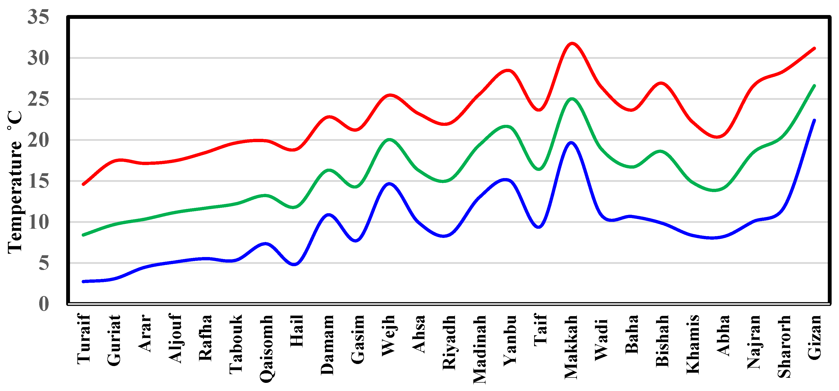
3.2. WAT Tnalysis
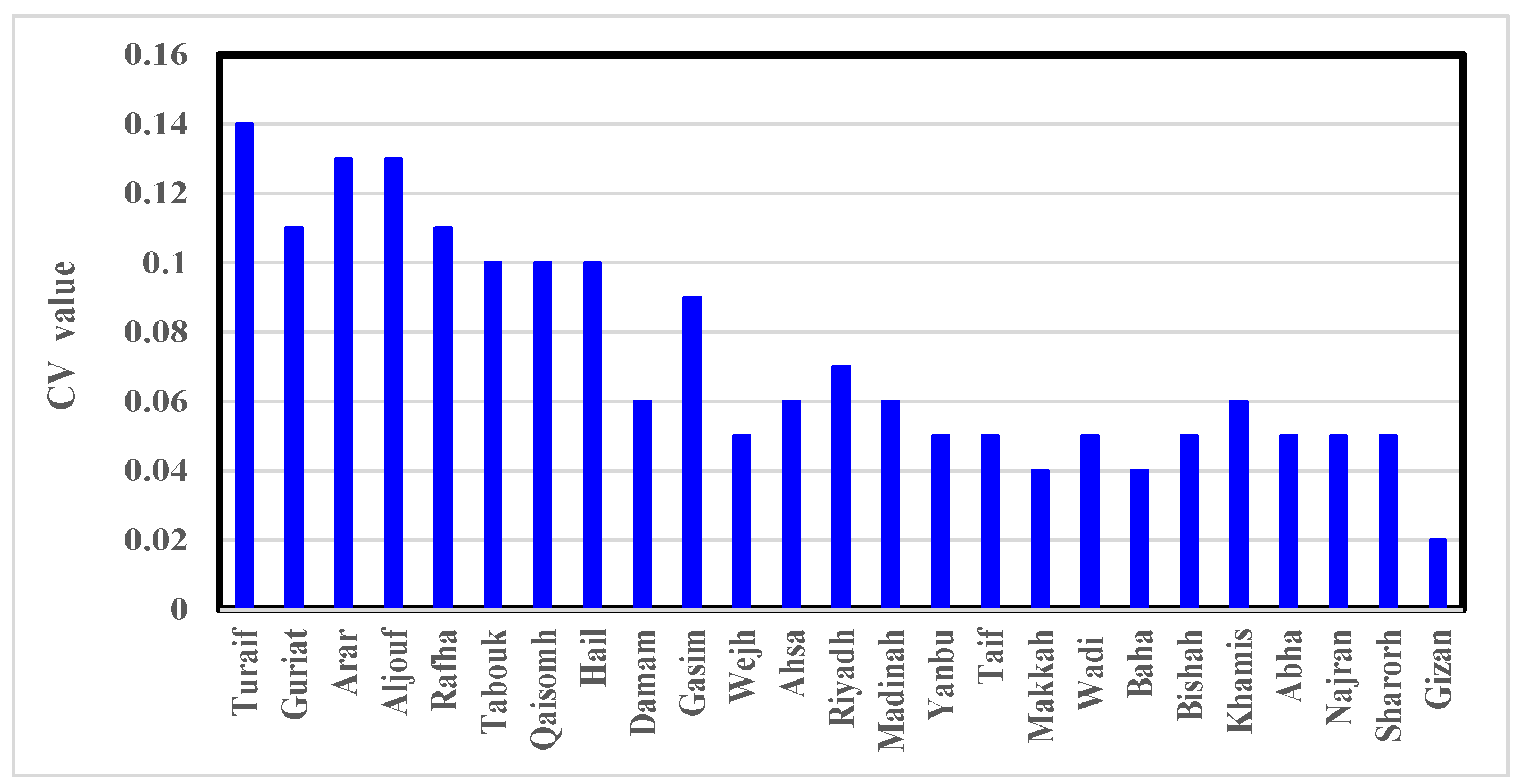
3.3. Coefficient of Variation
3.4. Trend Analysis
3.5. Cumulative Seasonal Means
3.6. Abrupt Change Analysis
3.7. Spatial Analysis of WAT
4. Conclusions
Author Contributions
Funding
Institutional Review Board Statement
Informed Consent Statement
Data Availability Statement
Acknowledgments
Conflicts of Interest
References
- Vinnikov, K.Y.; Groisman, P.Y.; Lugina, K.M. Empirical Data on Contemporary Global Climate Changes (Temperature and Precipitation). J. Clim. 1990, 3, 662–677. [Google Scholar] [CrossRef]
- Ponce, C. Intra-seasonal climate variability and crop diversification strategies in the Peruvian Andes: A word of caution on the sustainability of adaptation to climate change. World Dev. 2020, 127, 104740. [Google Scholar] [CrossRef]
- Folland, C.K.; Karl, T.P.; Christy, J.R.; Clarke, R.A.; Gruza, G.V.; Jouzel, J.; Mann, M.E.; Oerlemans, J.; Salinger, M.J.; Wang, S.W. Observed climate variability and change. In Chapter 2 of Climate Change 2001; The Scientific Basis, Contribution of Working Group I to the Third Assessment Report of the Intergovernmental Panel on Climate Change (IPCC); Houghton, J.T., Ding, Y., Griggs, D.J., Noguer, M., van der Linden, P.J., Xiaoxu, D., Eds.; Cambridge University Press: Cambridge, UK, 2001; pp. 99–181. [Google Scholar]
- Trenberth, K.E.; Fasullo, J.T. An apparent hiatus in global warming? Earth’s Future 2013, 1, 19–32. [Google Scholar] [CrossRef]
- IPCC. Climate change 2013: The Physical Science Basis. In Contribution of Working Group I to the Fifth Assessment Report of the Intergovernmental Panel on Climate Change; Stocker, T.F., Qin, D., Plattner, G.K., Tignor, M., Allen, S.K., Boschung, J., Nauels, A., Xia, Y., Bex, V., Midgley, P.M., Eds.; Cambridge University Press: Cambridge, UK; New York, NY, USA, 2013; p. 1535. [Google Scholar]
- Paeth, H.; Born, K.; Girmes, R.; Podzun, R.; Jacob, D. Regional Climate Change in Tropical and Northern Africa due to Greenhouse Forcing and Land Use Changes. J. Clim. 2009, 22, 114–132. [Google Scholar] [CrossRef] [Green Version]
- Fontaine, B.; Janicot, S.; Monerie, P.A. Recent changes in air temperature, heat waves occurrences, and atmospheric circulation in Northern Africa. J. Geophys. Res.-Atmos. 2013, 118, 8536–8552. [Google Scholar] [CrossRef]
- El Kenawy, A.; López-Moreno, J.I.; McCabe, M.F.; Brunsell, N.A.; Vicente-Serrano, S.M. Daily Temperature Changes and Variability in ENSEMBLES Regional Models Predictions: Evaluation and Intercomparison for the Ebro Valley (NE Iberia). Atmos. Res. 2015, 155, 141–157. [Google Scholar] [CrossRef] [Green Version]
- Almazroui, M.; Islam, M.N.; Jones, P.D.; Athar, H.; Rahman, M.A. Recent climate change in the Arabian Peninsula: Seasonal rainfall and temperature climatology of Saudi Arabia for 1979–2009. Atmos. Res. 2012, 111, 29–45. [Google Scholar] [CrossRef]
- Athar, H. Trends in observed extreme climate indices in Saudi Arabia during 1979–2008. Int. J. Climatol. 2014, 34, 1561–1574. [Google Scholar] [CrossRef]
- Almazroui, M.; Islam, M.N.; Dambul, R.; Jones, P.D. Trends of temperature extremes in Saudi Arabia. Int. J. Climatol. 2014, 34, 808–826. [Google Scholar] [CrossRef]
- Islam, M.N.; Almazroui, M.; Dambul, R.; Jones, P.D.; Alamoudi, A.O. Long-term changes in seasonal temperature extremes over Saudi Arabia during 1981–2010. Int. J. Climatol. 2015, 15, 1579–1592. [Google Scholar] [CrossRef]
- Raggad, B. Statistical assessment of changes in extreme maximum temperatures over Saudi Arabia, 1985–2014. Theor. Appl. Climatol. 2018, 132, 1217–1235. [Google Scholar] [CrossRef]
- Alhathloul, S.H.; Khan, A.A.; Mishra, A.K. Trend and change point detection in mean annual and seasonal maximum temperatures over Saudi Arabia. Arab. J. Geosci. 2021, 14, 1–6. [Google Scholar] [CrossRef]
- Hasanean, H.M.; Almazroui, M. Teleconnections of the tropical sea surface temperatures to the surface air temperature over Saudi Arabia in summer season. Int. J. Climatol. 2016, 37, 1040–1049. [Google Scholar] [CrossRef]
- Hasanean, H.M. Wintertime surface temperature in Egypt in relation to the associated atmospheric circulation. Int. J. Climatol. 2004, 24, 985–999. [Google Scholar] [CrossRef]
- Domroes, M.; El-Tantawi, A. Recent temporal and spatial temperature changes in Egypt. Int. J. Climatol. 2005, 25, 51–63. [Google Scholar] [CrossRef]
- Hasanean, H.M.; Abdel-Basset, H. Variability of summer temperature over Egypt. Int. J. Climatol. 2006, 26, 1619–1634. [Google Scholar] [CrossRef]
- El Kenawy, A.; López-Moreno, J.I.; Vicente-Serrano, S.M.; Abd-Elaal, M. Temperature variability along the Mediterranean Coast and its links to Large Scale Atmospheric Circulations (1957–2006). Bull. De La Soc. De Geogr. D’Egypte 2010, 83, 12–26. [Google Scholar]
- El Kenawy, A.; López-Moreno, J.I.; Vicente-Serrano, S.M.; Mekld, M.S. Temperature trends in Libya over the second half of the 20th century. Theor. Appl. Climatol. 2009, 98, 1–8. [Google Scholar] [CrossRef]
- Khomsi, K.; Mahe, G.; Tramblay, Y.; Sinan, M.; Snoussi, M. Regional impacts of global change: Seasonal trends in extreme rainfall, run-off and temperature in two contrasting regions of Morocco. Nat. Hazards Earth Syst. Sci. 2016, 16, 1079–1090. [Google Scholar] [CrossRef] [Green Version]
- Zhang, X.; Aguilar, E.; Sensoy, S.; Melkonyan, H.; Tagiyeva, U.; Ahmed, N.; Kutaladze, N.; Rahimzadeh, F.; Taghipour, A.; Hantosh, T.; et al. Trends in Middle East climate extreme indices from 1950 to 2003. J. Geophys. Res. 2005, 110, D22104. [Google Scholar] [CrossRef]
- Wang, X.J.; Zhang, J.Y.; Shahid, S.; Guan, E.H.; Wu, Y.X.; Gao, J.; He, R.M. Adaptation to climate change impacts on water demand. Mitig. Adapt. Strateg. Glob. Chang. 2016, 21, 81–99. [Google Scholar] [CrossRef]
- World Bank. Making the Most of Scarcity: Accountability for Better Water Management Results in the Middle East and North Africa Report; World Bank: Washington, DC, USA, 2010. [Google Scholar]
- Al-Zahrani, K.H.; Baig, M.B. Water in the Kingdom of Saudi Arabia: Sustainable management options. J. Anim. Plant Sci. 2011, 21, 601–604. [Google Scholar]
- Kaniewski, D.; Van Campo, E.; Weiss, H. Drought is a recurring challenge in the Middle East. Proc. Natl. Acad. Sci. USA 2012, 109, 3862–3867. [Google Scholar] [CrossRef] [PubMed] [Green Version]
- Odhiambo, G.O. Water scarcity in the Arabian Peninsula and socio-economic implications. Appl. Water Sci. 2017, 7, 2479–2492. [Google Scholar] [CrossRef] [Green Version]
- Attada, R.; Dasari, H.P.; Parekh, A.; Chowdary, J.S.; Langodan, S.; Knio, O.; Ibrahim, H. The role of the Indian summer monsoon variability on Arabian Peninsula summer climate. Clim. Dyn. 2018, 52, 3389–3404. [Google Scholar] [CrossRef]
- Bannayan, M.; Sanjani, S.; Alizadeh, A.; Lotfabadi, S.S.; Mohamadian, A. Association between climate indices, aridity index, and rainfed crop yield in northeast of Iran. Field Crops Res. 2010, 118, 105–114. [Google Scholar] [CrossRef]
- Almazroui, M.; Hasanean, H.M.; Al-Khalaf, A.K.; Abdel Basset, H. Detecting climate change signals in Saudi Arabia using mean annual surface air temperatures. Theor. Appl. Climatol. 2013, 113, 585–598. [Google Scholar] [CrossRef]
- Kunchala, R.; Attada, R.; Dasari, H.P.; Vellore, R.K.; Langodan, S.; Abualnaja, Y.O.; Ibrahim, H. Aerosol optical depth variability over the Arabian Peninsula as inferred from satellite measurements. Atmos. Environ. 2018, 187, 346–357. [Google Scholar]
- Otterman, J.; Angell, J.K.; Ardizzone, J.; Atlas, R.; Schubert, S.; Starr, D.; Wu, M.L. North-Atlantic surface winds examined as the source of winter warming in Europe. Geophys. Res. Lett. 2002, 29, 18. [Google Scholar] [CrossRef]
- Croitoru, A.E.; Drignei, D.; Dragotă, C.S.; Imecs, Z.; Burada, D.C. Sharper detection of winter temperature changes in the Romanian higher-elevations. Glob. Planet. Chang. 2014, 122, 122–129. [Google Scholar] [CrossRef]
- Hillebrand, E.; Proietti, T. Phase changes and seasonal warming in early instrumental temperature records. J. Clim. 2017, 30, 6795–6821. [Google Scholar] [CrossRef]
- Zhao, C.; Gong, J.; Wang, H.; Wei, S.; Song, Q.; Zhou, Y. Changes of temperature and precipitation extremes in a typical arid and semiarid zone: Observations and multi-model ensemble projections. Int. J. Climatol. 2020, 40, 5128–5153. [Google Scholar] [CrossRef]
- Karl, T.R.; Jones, P.D.; Knight, R.W.; Kukla, G.; Plummer, N.; Razuvayev, V.; Gallo, K.P.; Lindseay, J.; Charlson, R.J.; Peterson, T.C. 1993 A new perspective on recent global warming: Asymmetric trends of daily maximum and minimum temperature. Bull. Am. Meteorol. Soc. 1993, 74, 1007–1024. [Google Scholar] [CrossRef]
- Houghton, J.T.; Meria, F.L.G.; Callander, B.A.; Harris, N.; Kattenberg, A.; Maskell, K. 1996 Climate Change. In The IPCC Second Assessment Report; Cambridge University Press: New York, NY, USA, 1996; p. 572. [Google Scholar]
- IPCC. Climate Change 2014: Mitigation of Climate Change. In Contribution of Working Group III to the Fifth Assessment Report of the Intergovernmental Panel on Climate Change; Edenhofer, O., Pichs-Madruga, R., Sokona, Y., Farahani, E., Kadner, S., Seyboth, K., Adler, A., Baum, I., Brunner, S., Eickemeier, P., et al., Eds.; Cambridge University Press: Cambridge, UK; New York, NY, USA, 2014. [Google Scholar]
- Chung, Y.S.; Yoon, M.B. Interpretation of recent temperature and precipitation trends observed in Korea. Theor. Appl. Climatol. 2000, 67, 171–180. [Google Scholar] [CrossRef]
- Quintana-Gomez, R.A. Trends of maximum and minimum temperatures in Northern South America. J. Clim. 1999, 12, 2104–2112. [Google Scholar] [CrossRef]
- Rahimzadeh, F.; Askari, A. Attitudinal differences between minimum and maximum rate of temperature and the decrease in diurnal temperature range in the country. J. Geogr. Res. 2004, 73, 155–171. [Google Scholar]
- Easterling, D.R.; Meehl, G.A.; Parmesanm, C.; Changnon, S.A.; Karl, T.R.; Mearns, L.O. Climate extremes: Observations, modeling, and impacts. Science 2000, 289, 2068–2074. [Google Scholar] [CrossRef] [PubMed] [Green Version]
- Alkolibi, F.M. Possible effects of global warming on agriculture and water resources in Saudi Arabia: Impacts and responses. Clim. Chang. 2002, 54, 225–245. [Google Scholar] [CrossRef]
- Walther, G.R.; Post, E.; Convey, P.; Menzel, A.; Parmesan, C.; Beebee, T.J.C.; Fromentin, J.M.; Hoegh-Guldberg, O.; Bairlein, F. Ecological responses to recent climate change. Nature 2002, 416, 389–395. [Google Scholar] [CrossRef] [PubMed]
- Alghamdi, A.S.; Moore, T.W. Analysis and comparison of trends in extreme temperature indices in Riyadh City, Kingdom of Saudi Arabia, 1985–2010. J. Climatol. 2014, 1, 1–10. [Google Scholar] [CrossRef] [Green Version]
- Almazroui, M. RegCM4 in climate simulation over CORDEX-MENA/Arab domain: Selection of suitable domain, convection and land surface schemes. Int. J. Climatol. 2016, 36, 236–351. [Google Scholar] [CrossRef]
- Hersbach, H.; Bell, B.; Berrisford, P.; Hirahara, S.; Horányi, A.; Muñoz-Sabater, J.; Nicolas, J.; Peubey, C.; Radu, R.; Schepers, D.; et al. The ERA5 global reanalysis. Q. J. R. Meteorol. Soc. 1999, 146, 2049. [Google Scholar] [CrossRef]
- Bartlett, M.S. Properties of sufficiency and statistical tests. Proceedings of the Royal Society of London. Ser. A Math. Phys. Sci. 1937, 160, 268–282. [Google Scholar]
- Mitchell, J.M.; Dzerdzeevskii, B.; Flohn, H.; Hofmery, W.L. Climatic change. In WMO Tech. Note 79. WMO No. 195. TP-100; World Meteorological Organization: Geneva, Switzerland, 1966; p. 79. [Google Scholar]
- Pearson, E.S.; Hartley, H.O. Biometrika Tables for Statisticians; Cambridge University Press: Cambridge, UK, 1958; 240p. [Google Scholar]
- Panofsky, H.A.; Brier, G.W. Some Applications of Statistics to Meteorology; Pennsylvania State University Press: University Park, PA, USA, 1963; p. 224. [Google Scholar]
- McBean, E.; Motiee, H. Assessment of impact of climate change on water resources. Hydrol. Earth Syst. Sci. 2008, 12, 239–255. [Google Scholar] [CrossRef] [Green Version]
- Sen, P.K. Estimates of the regression coefficient based on Kendall’s. J. Am. Stat. Assoc. 1968, 63, 1379–1389. [Google Scholar] [CrossRef]
- Mann, H.B. Nonparametric tests against trend. Econometrica 1945, 13, 245–259. [Google Scholar] [CrossRef]
- Kendall, M.G. Rank Correlation Methods; Griffin: Salisbury South, SA, Australia, 1948. [Google Scholar]
- Sonali, P.; Kumar, D.N. Review of trend detection methods and their application to detect temperature changes in India. J. Hydrol. 2013, 476, 212–227. [Google Scholar] [CrossRef]
- Von Storch, H. Misuses of statistical analysis in climate. In Analysis of Climate Variability: Applications of Statistical Techniques; Von Storch, H., Navarra, A., Eds.; Springer: Berlin/Heidelberg, Germany, 1995; pp. 11–26. [Google Scholar]
- Hamed, K.H.; Rao, A.R. A modified Mann-Kendall trend test for autocorrelated data. J. Hydrol. 1998, 204, 182–196. [Google Scholar] [CrossRef]
- Hamed, K.H. Trend detection in hydrologic data: The Mann–Kendall trend test under the scaling hypothesis. J. Hydrol. 2008, 349, 350–363. [Google Scholar] [CrossRef]
- Al-Kallas, S.; Al-Mutairi, M.; Abdel Basset, H.; Abdeldym, A.; Morsy, M.; Badawy, A. Climatological Study of Ozone over Saudi Arabia. Atmosphere 2021, 12, 1275. [Google Scholar] [CrossRef]
- Kamel, A.M.; Abdel Basset, H.; Sayad, T. Rainfall analysis and variability over Egypt. Al-Azhar Bull. Sci. 2017, 28, 41–62. [Google Scholar]
- Pavia, E.G.; Graef, F. The recent rainfall climatology of the Mediterranean Californias. J. Clim. 2002, 15, 2697–2701. [Google Scholar] [CrossRef]
- Mann, H.B.; Whitney, D.R. On a test of whether one of two random variables is stochastically larger than the other. Ann. Math. Stat. 1947, 18, 50–60. [Google Scholar] [CrossRef]
- Conover, W.J. Practical Nonparametric Statistics, 1st ed.; John Wiley & Sons: New York, NY, USA, 1971; pp. 97–104. [Google Scholar]
- Mendenhall, W.; Wackerly, D.D.; Sheaffer, R.L. Mathematical Statistics with Applications, 4th ed.; PWS-Kent: Boston, MA, USA, 1990. [Google Scholar]
- Sayad, T.A.; Ali, A.M.; Kamel, A.M. Study the impact of climate change on maximum and minimum temperature over Alexandria, Egypt using statistical downscaling model (SDSM). Glob. J. Adv. Res. 2016, 3, 694–712. [Google Scholar]
- Yan, M.H.; Deng, W.; Chen, P.Q. Analysis of climate jumps in the Sanjiang Plain. Sci. Geogr. Sin. 2003, 23, 661–667. [Google Scholar]
- Fu, C.; Wang, Q. The defnition and detection of the abrupt climatic change. Sci. Atmos. A Sin. 1992, 16, 482–493. [Google Scholar]
- Vorhees, D.C. The Impact of Global Scale Climate Variation on Southwest Asia. Master’s Thesis, Naval Postgraduate School, Monterey, CA, USA, 2006. [Google Scholar]


 The means of CSM and
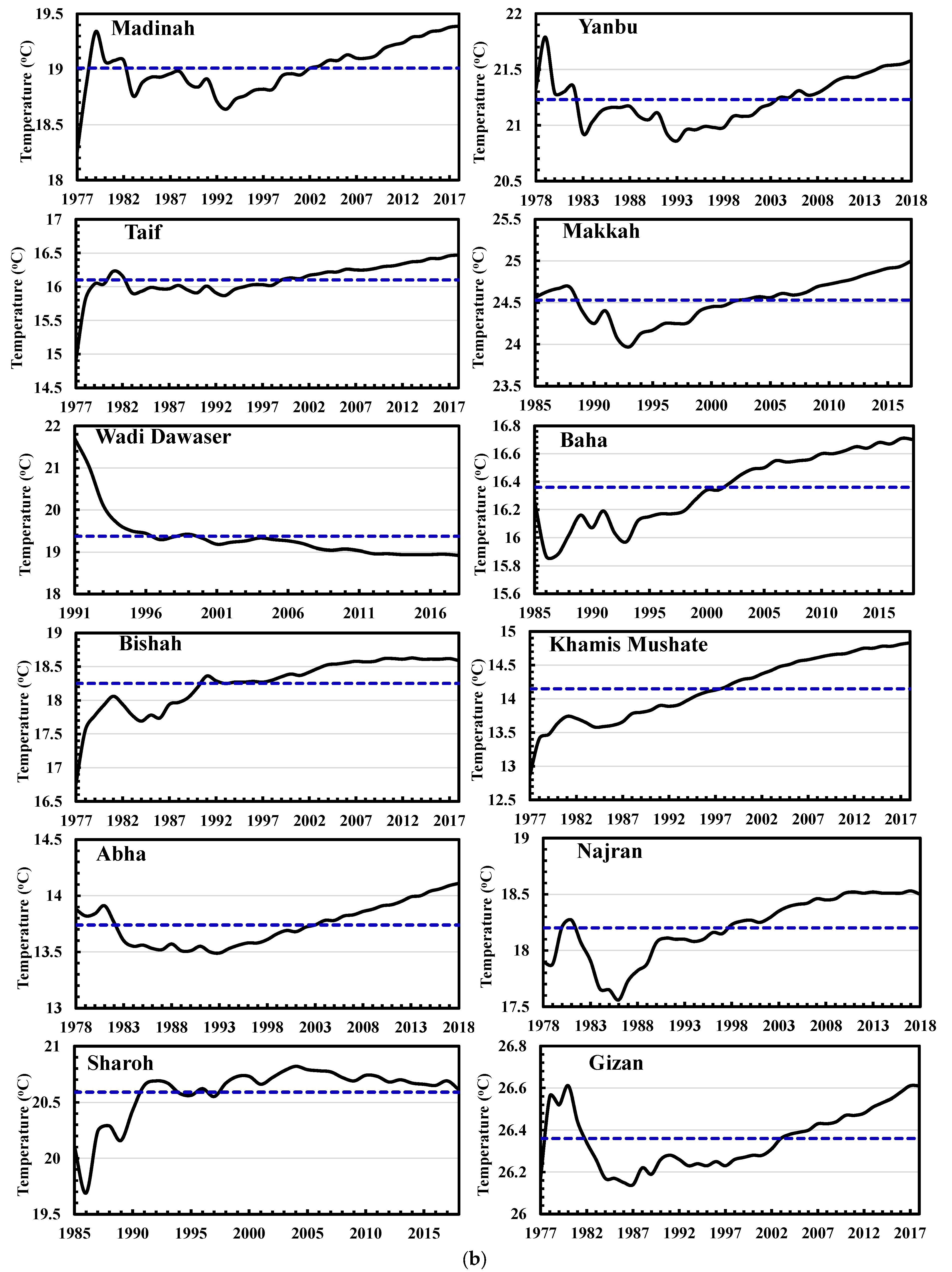
  the CSM time series. The stations are arranged from north to south. (b) As in (a) but for the stations Madinha, Yanbu, Taif, Makkah, Wadi Dawaser, Baha, Bishah, Khamis Mushate, Abha, Najran, Sharoh and Gizan.
The means of CSM and the CSM time series. The stations are arranged from north to south. (b) As in (a) but for the stations Madinha, Yanbu, Taif, Makkah, Wadi Dawaser, Baha, Bishah, Khamis Mushate, Abha, Najran, Sharoh and Gizan.
the CSM time series. The stations are arranged from north to south. (b) As in (a) but for the stations Madinha, Yanbu, Taif, Makkah, Wadi Dawaser, Baha, Bishah, Khamis Mushate, Abha, Najran, Sharoh and Gizan.
The means of CSM and the CSM time series. The stations are arranged from north to south. (b) As in (a) but for the stations Madinha, Yanbu, Taif, Makkah, Wadi Dawaser, Baha, Bishah, Khamis Mushate, Abha, Najran, Sharoh and Gizan.
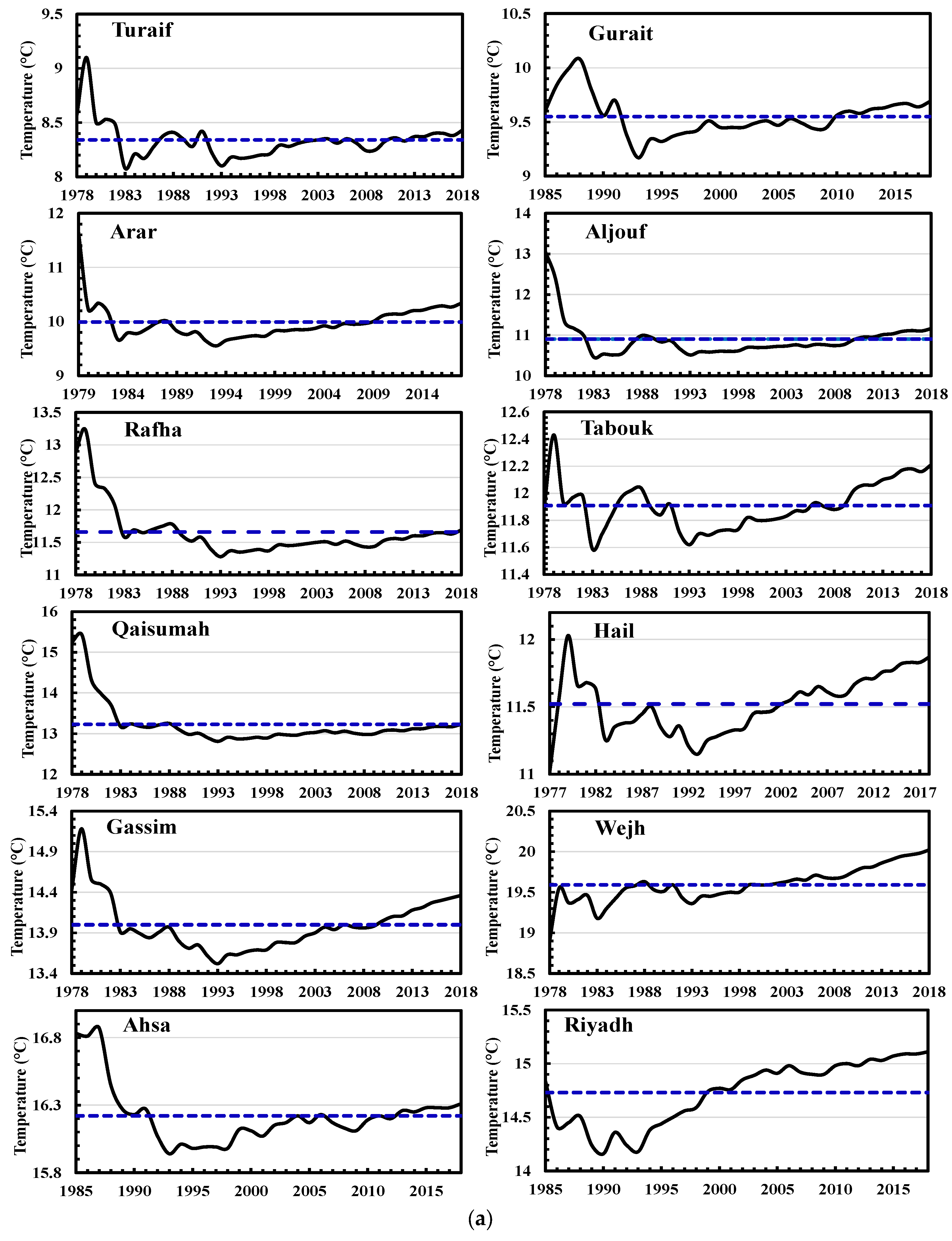
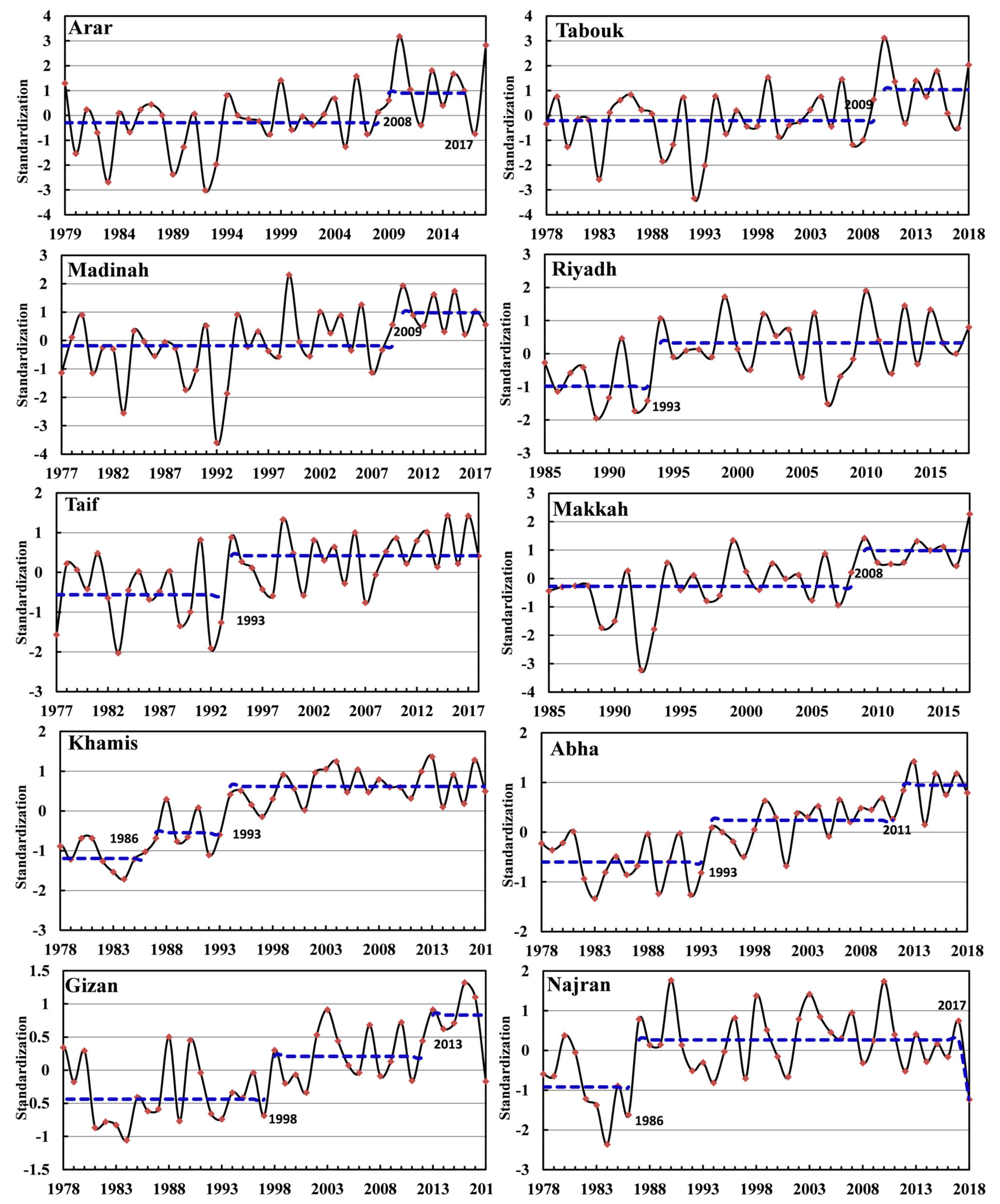
 Weighted arithmetic means and
  the standardization time series.
Weighted arithmetic means and the standardization time series.
the standardization time series.
Weighted arithmetic means and the standardization time series.


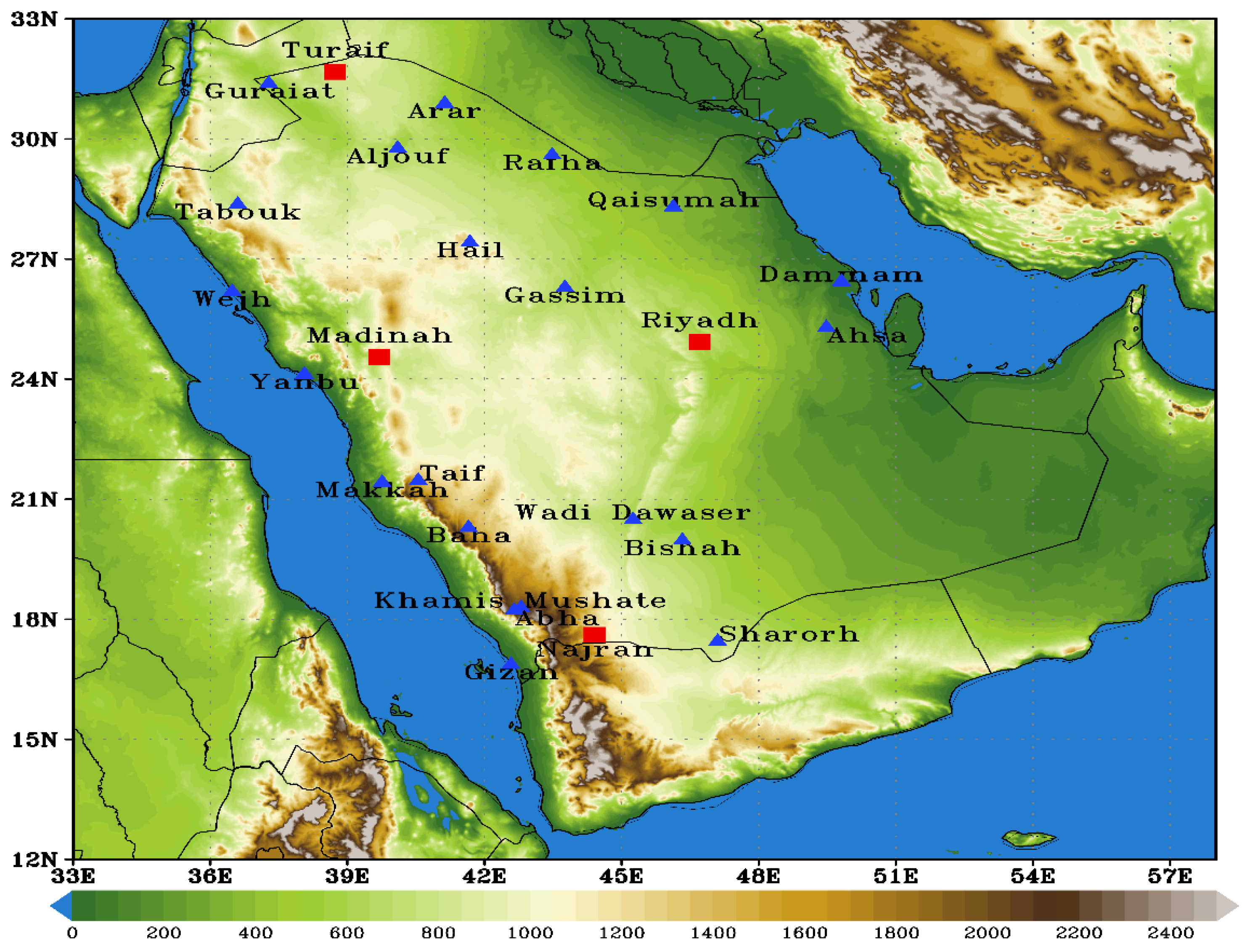
| No. | Station Name | Latitude | Longitude | Elevation (m) | Available Data |
|---|---|---|---|---|---|
| 1 | Turaif | 31.68° N | 38.73° E | 855 | 1978–2018 |
| 2 | Guriat | 31.40° N | 37.28° E | 509 | 1985–2018 |
| 3 | Arar | 30.90° N | 41.13° E | 555 | 1979–2018 |
| 4 | Aljouf | 29.78° N | 40.10° E | 689 | 1978–2018 |
| 5 | Rafha | 29.61° N | 43.48° E | 449 | 1978–2018 |
| 6 | Tabouk | 28.38° N | 36.60° E | 778 | 1978–2018 |
| 7 | Qaisumah | 28.31° N | 46.13° E | 358 | 1978–2018 |
| 8 | Hail | 27.43° N | 41.68° E | 1015 | 1977–2018 |
| 9 | Damam | 26.45° N | 49.81° E | 22 | 2000–2018 |
| 10 | Gassim | 26.30° N | 43.76° E | 648 | 1978–2018 |
| 11 | Wejh | 26.20° N | 36.48° E | 20 | 1978–2018 |
| 12 | Ahsa | 25.30° N | 49.48° E | 179 | 1985–2018 |
| 13 | Riyadh | 24.93° N | 46.71° E | 614 | 1985–2018 |
| 14 | Madinah | 24.55° N | 39.70° E | 654 | 1977–2018 |
| 15 | Yanbu | 24.13° N | 38.06° E | 8 | 1978–2018 |
| 16 | Taif | 21.48° N | 40.55° E | 1478 | 1977–2018 |
| 17 | Makkah | 21.43° N | 39.76° E | 240 | 1985–2018 |
| 18 | Wadi Dawaser | 20.50° N | 45.25° E | 629 | 1991–2018 |
| 19 | Baha | 20.30° N | 41.65° E | 1672 | 1985–2018 |
| 20 | Bishah | 19.98° N | 46.33° E | 1167 | 1977–2018 |
| 21 | Khamis Mushate | 18.30° N | 42.80° E | 2066 | 1977–2018 |
| 22 | Abha | 18.23° N | 42.65° E | 2090 | 1978–2018 |
| 23 | Najran | 17.61° N | 44.41° E | 1214 | 1978–2018 |
| 24 | Sharorh | 17.46° N | 47.10° E | 720 | 1985–2018 |
| 25 | Gizan | 16.88° N | 42.58° E | 6 | 1977–2018 |
| No. | Station Name | m | K | 95% Significant Point | Homogenity of WAT | No. | Station Name | m | K | 95% Significant Point | Homogenity of WAT |
|---|---|---|---|---|---|---|---|---|---|---|---|
| 1 | Turaif | 13 | 3 | 4.16 | 3.575 | 14 | Madinah | 13 | 3 | 4.16 | 4.05 |
| 2 | Guriat | 11 | 3 | 4.85 | 0.07 | 15 | Yanbu | 13 | 3 | 4.16 | 4.08 |
| 3 | Arar | 13 | 3 | 4.16 | 0.97 | 16 | Taif | 13 | 3 | 4.16 | 2.89 |
| 4 | Aljouf | 13 | 3 | 4.16 | 0.49 | 17 | Makkah | 11 | 3 | 4.85 | 0.14 |
| 5 | Rafha | 13 | 3 | 4.16 | 0.82 | 18 | Wadi Dawaser | 9 | 3 | 6.00 | 0.56 |
| 6 | Tabouk | 13 | 3 | 4.16 | 2.07 | 19 | Baha | 11 | 3 | 4.85 | 0.22 |
| 7 | Qaisumah | 13 | 3 | 4.16 | 0.35 | 20 | Bishah | 13 | 3 | 4.16 | 1.69 |
| 8 | Hail | 13 | 3 | 4.16 | 2.12 | 21 | Khamis Mushate | 13 | 3 | 4.16 | 1.34 |
| 9 | Damam | 7 | 3 | 8.38 | 2.82 | 22 | Abha | 13 | 3 | 4.16 | 3.38 |
| 10 | Gassim | 13 | 3 | 4.16 | 1.01 | 23 | Najran | 13 | 3 | 4.16 | 0.24 |
| 11 | Wejh | 13 | 3 | 4.16 | 3.21 | 24 | Sharorh | 11 | 3 | 4.85 | 1.26 |
| 12 | Ahsa | 11 | 3 | 4.85 | 1.79 | 25 | Gizan | 13 | 3 | 4.16 | 0.46 |
| 13 | Riyadh | 11 | 3 | 4.85 | 0.41 | ||||||
| No. | Station Name | SLR (°C/Year) | SS (°C/Year) | p Value | Tau | Trend Direction |
|---|---|---|---|---|---|---|
| 1 | Turaif | 0.017 | 0.012 | 0.019 | 0.08 | + and S |
| 2 | Guriat | 0.026 | 0.02 | 0.003 | 0.13 | + and S |
| 3 | Arar | 0.053 | 0.049 | 0 | 0.279 | + and S |
| 4 | Aljouf | 0.047 | 0.048 | 0 | 0.257 | + and S |
| 5 | Rafha | 0.022 | 0.02 | 0.086 | 0.085 | + and NS |
| 6 | Tabouk | 0.041 | 0.037 | 0 | 0.229 | + and S |
| 7 | Qaisumah | 0.023 | 0.03 | 0.002 | 0.156 | + and S |
| 8 | Hail | 0.042 | 0.039 | 0 | 0.28 | + and S |
| 9 | Damam | 0.024 | 0.031 | 0.101 | 0.099 | + and NS |
| 10 | Gassim | 0.055 | 0.057 | 0 | 0.333 | + and S |
| 11 | Wejh | 0.048 | 0.046 | 0 | 0.388 | + and S |
| 12 | Ahsa | 0.021 | 0.02 | 0.001 | 0.125 | + and S |
| 13 | Riyadh | 0.043 | 0.044 | 0 | 0.289 | + and S |
| 14 | Madinah | 0.044 | 0.04 | 0 | 0.324 | + and S |
| 15 | Yanbu | 0.045 | 0.04 | 0 | 0.328 | + and S |
| 16 | Taif | 0.037 | 0.038 | 0 | 0.364 | + and S |
| 17 | Makkah | 0.071 | 0.063 | 0 | 0.466 | + and S |
| 18 | Wadi Dawaser | −0.046 | −0.04 | 0 | −0.198 | - and S |
| 19 | Baha | 0.038 | 0.035 | 0 | 0.38 | + and S |
| 20 | Bishah | 0.022 | 0.023 | 0.001 | 0.217 | + and S |
| 21 | Khamis Mushate | 0.061 | 0.063 | 0 | 0.609 | + and S |
| 22 | Abha | 0.044 | 0.044 | 0 | 0.6 | + and S |
| 23 | Najran | 0.024 | 0.021 | 0.002 | 0.202 | + and S |
| 24 | Sharorh | −0.013 | −0.01 | 0.262 | −0.059 | − and NS |
| 25 | Gizan | 0.031 | 0.034 | 0 | 0.459 | + and S |
| Year | Stations | Types of the Abrupt |
|---|---|---|
| 1986 | Bishah–Khamis Mushate–Najran | Warming |
| 1993 | Riyadh–Taif–Baha–Khamis Mushate–Abha | Warming |
| 1998 | Gizan | Warming |
| 2001 | Yanbu | Warming |
| 2006 | Wadi Dawaser | Cooling |
| 2008 | Arar–Aljouf–Makkah | Warming |
| 2009 | Tabouk–Hail–Gassim–Wejh–Madinah | Warming |
| 2011 | Abha | Warming |
| 2013 | Gizan | Warming |
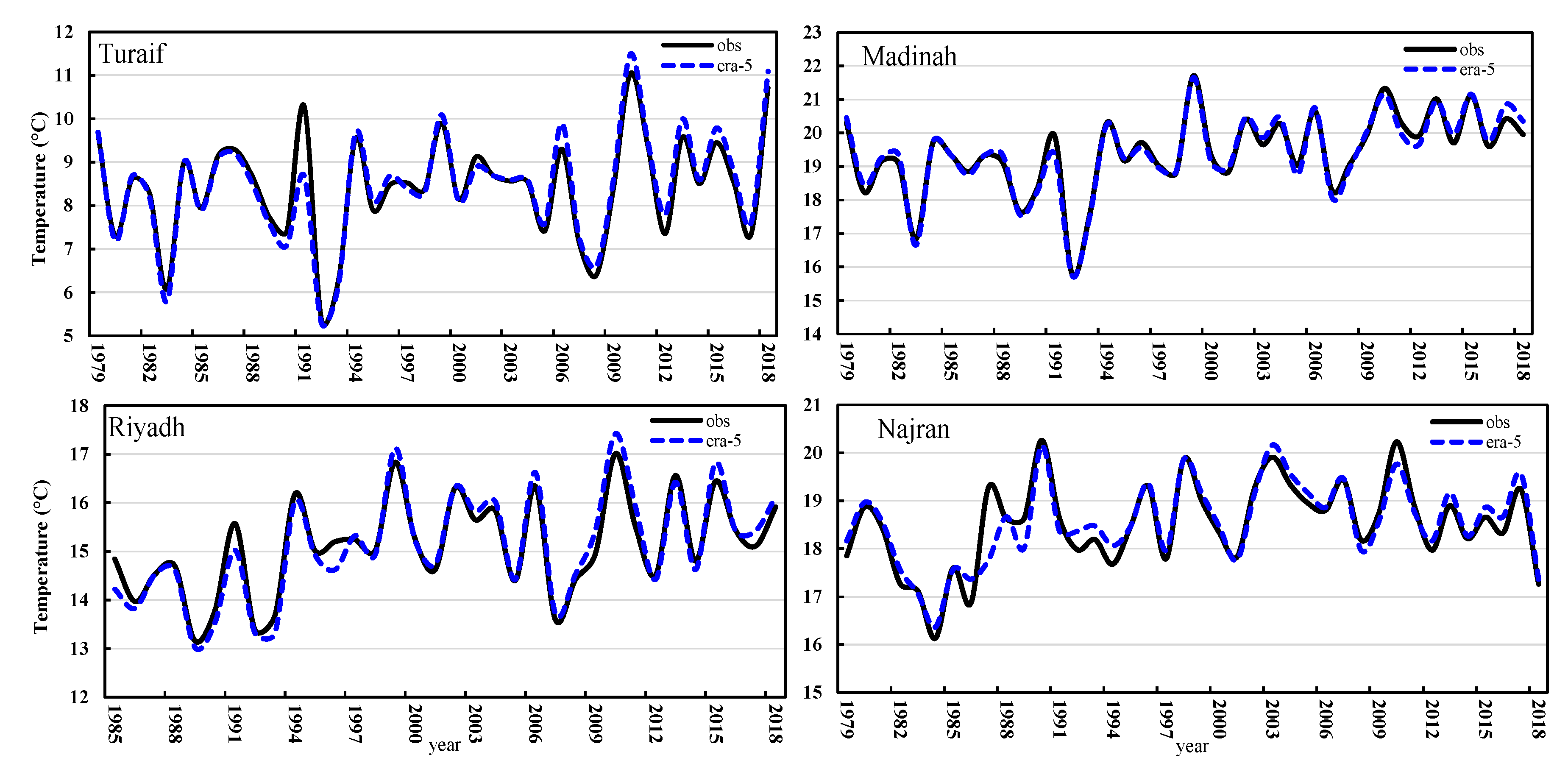
| Station Name | R | d | R2 | RMSE | MBE | MPE% |
|---|---|---|---|---|---|---|
| Turaif | 0.96 | 0.95 | 0.93 | 0.337 | −0.032 | 0.38 |
| Madinah | 0.99 | 0.98 | 0.97 | 0.197 | 2.21 × 10⁻¹⁴ | 1.13 × 10⁻¹³ |
| Riyadh | 0.97 | 0.95 | 0.95 | 0.271 | 5.88 × 10⁻⁵ | 0.0004 |
| Najran | 0.93 | 0.91 | 0.86 | 0.339 | −0.64 | −0.22 |
Disclaimer/Publisher’s Note: The statements, opinions and data contained in all publications are solely those of the individual author(s) and contributor(s) and not of MDPI and/or the editor(s). MDPI and/or the editor(s) disclaim responsibility for any injury to people or property resulting from any ideas, methods, instructions or products referred to in the content. |
© 2023 by the authors. Licensee MDPI, Basel, Switzerland. This article is an open access article distributed under the terms and conditions of the Creative Commons Attribution (CC BY) license (https://creativecommons.org/licenses/by/4.0/).
Share and Cite
Al-Mutairi, M.; Labban, A.; Abdeldym, A.; Abdel Basset, H. Trend Analysis and Fluctuations of Winter Temperature over Saudi Arabia. Climate 2023, 11, 67. https://doi.org/10.3390/cli11030067
Al-Mutairi M, Labban A, Abdeldym A, Abdel Basset H. Trend Analysis and Fluctuations of Winter Temperature over Saudi Arabia. Climate. 2023; 11(3):67. https://doi.org/10.3390/cli11030067
Chicago/Turabian StyleAl-Mutairi, Motirh, Abdulhaleem Labban, Abdallah Abdeldym, and Heshmat Abdel Basset. 2023. "Trend Analysis and Fluctuations of Winter Temperature over Saudi Arabia" Climate 11, no. 3: 67. https://doi.org/10.3390/cli11030067