
Potential Impacts of Climate Change on Surface Water Resources in Arid Regions Using Downscaled Regional Circulation Model and Soil Water Assessment Tool, a Case Study of Amman-Zerqa Basin, Jordan


Abstract
:1. Introduction
2. Materials and Methods
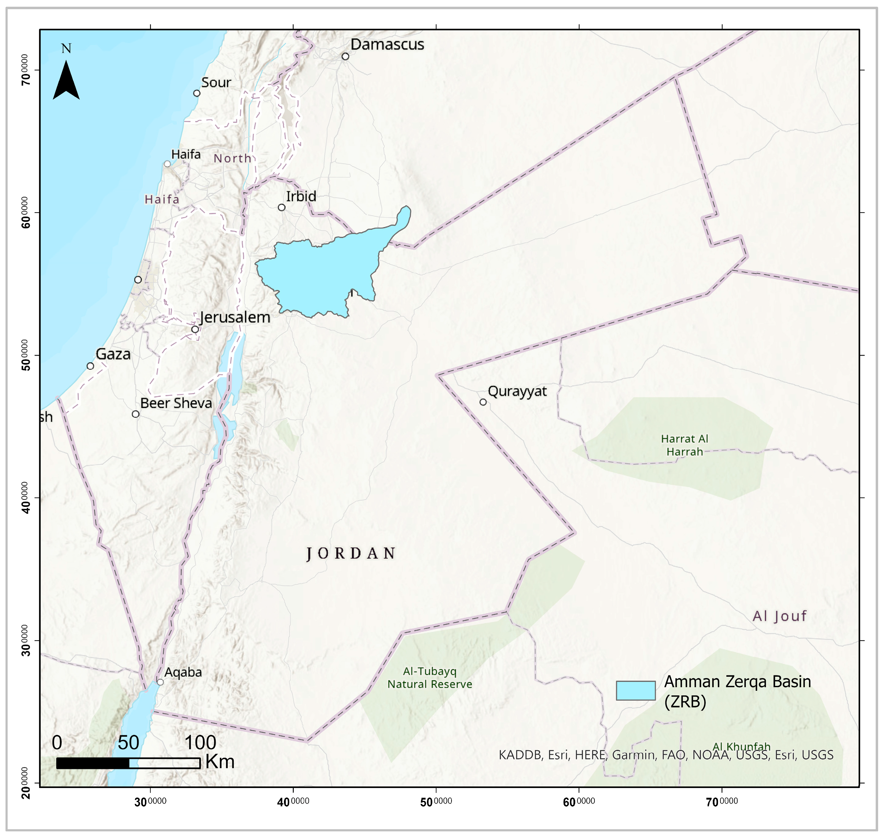
2.1. Study Area
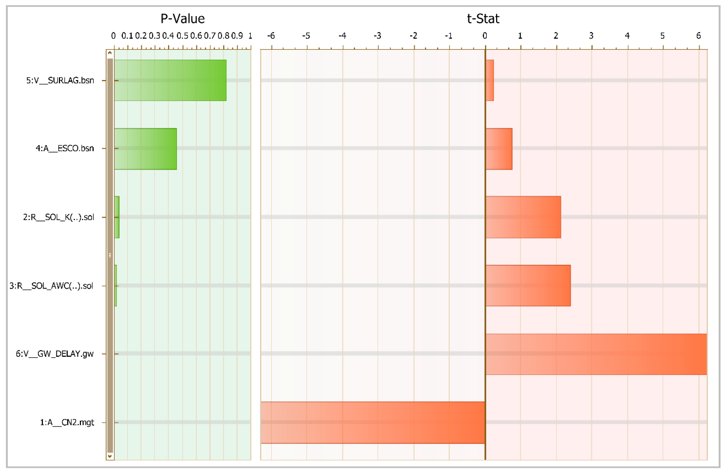
2.2. SWAT Modeling
2.3. Development of Reference Scenario Using SWAT
- Nash-Sutcliffe efficiency (NSE): determines the relative magnitude of the residual variance compared to the measured data variance [23]. Its value ranges from −∞ to 1, where 1 indicates a perfect model and a value less than 0 indicates that the mean value of the observed time series would have been a better predictor than the model.where Qi is the measured discharge on day i, is the simulated discharge on day i, and is the mean measured discharge.
- Percent bias (PBIAS): measures the difference between the simulated and observed quantity, and its optimum value is 0. A positive value of the model represents underestimation, whereas a negative value represents the model overestimation [23].
- The ratio of the root-mean-square error to the standard deviation of measured data (RSR): a complementary indicator to RMSE, it standardizes the RMSE using the observation standard deviation. The optimum value of RSR is 0 and a higher value indicates lower model performance [23].
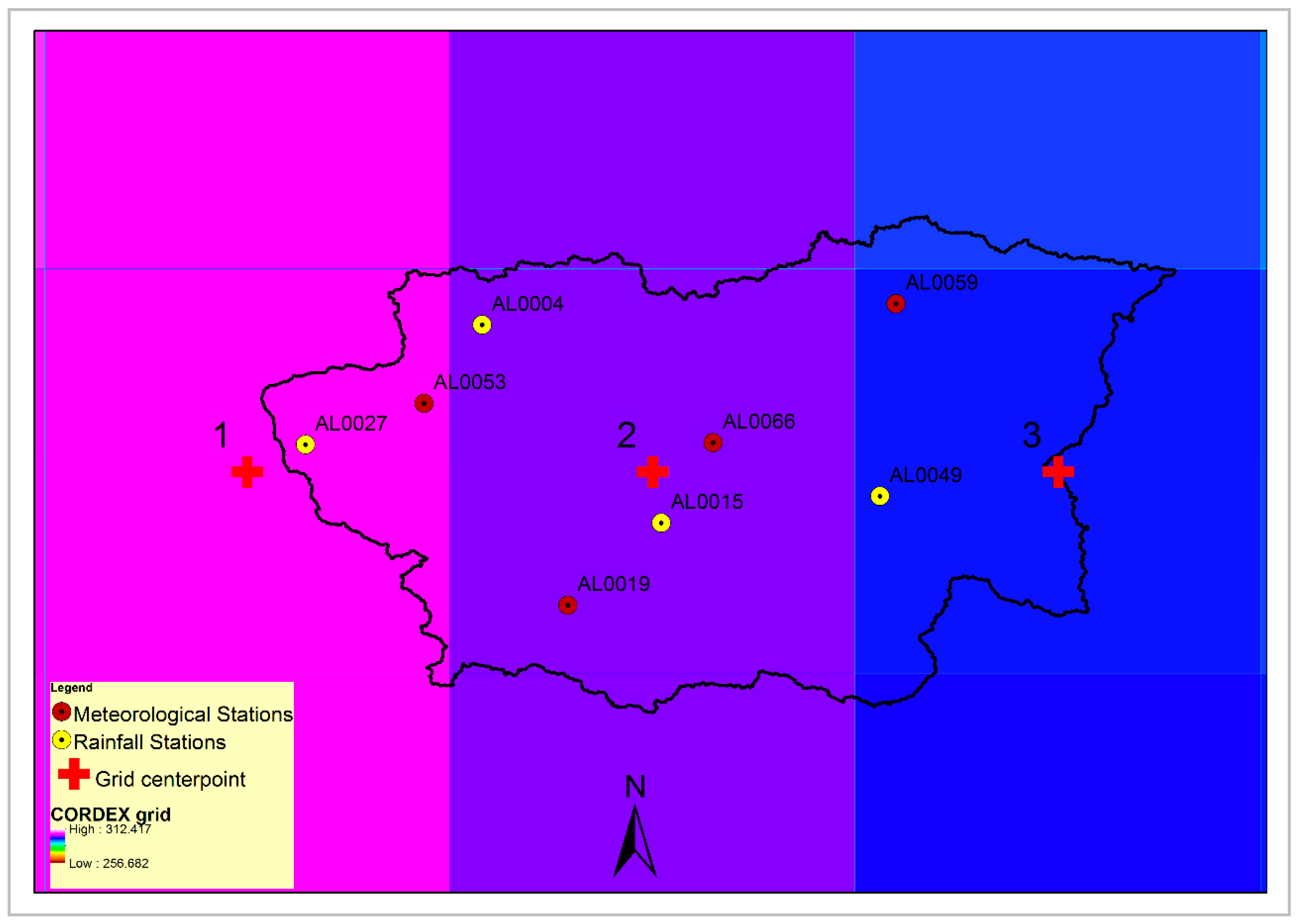
2.4. Climate Model Analysis and Future Scenario Development
3. Results and Discussion
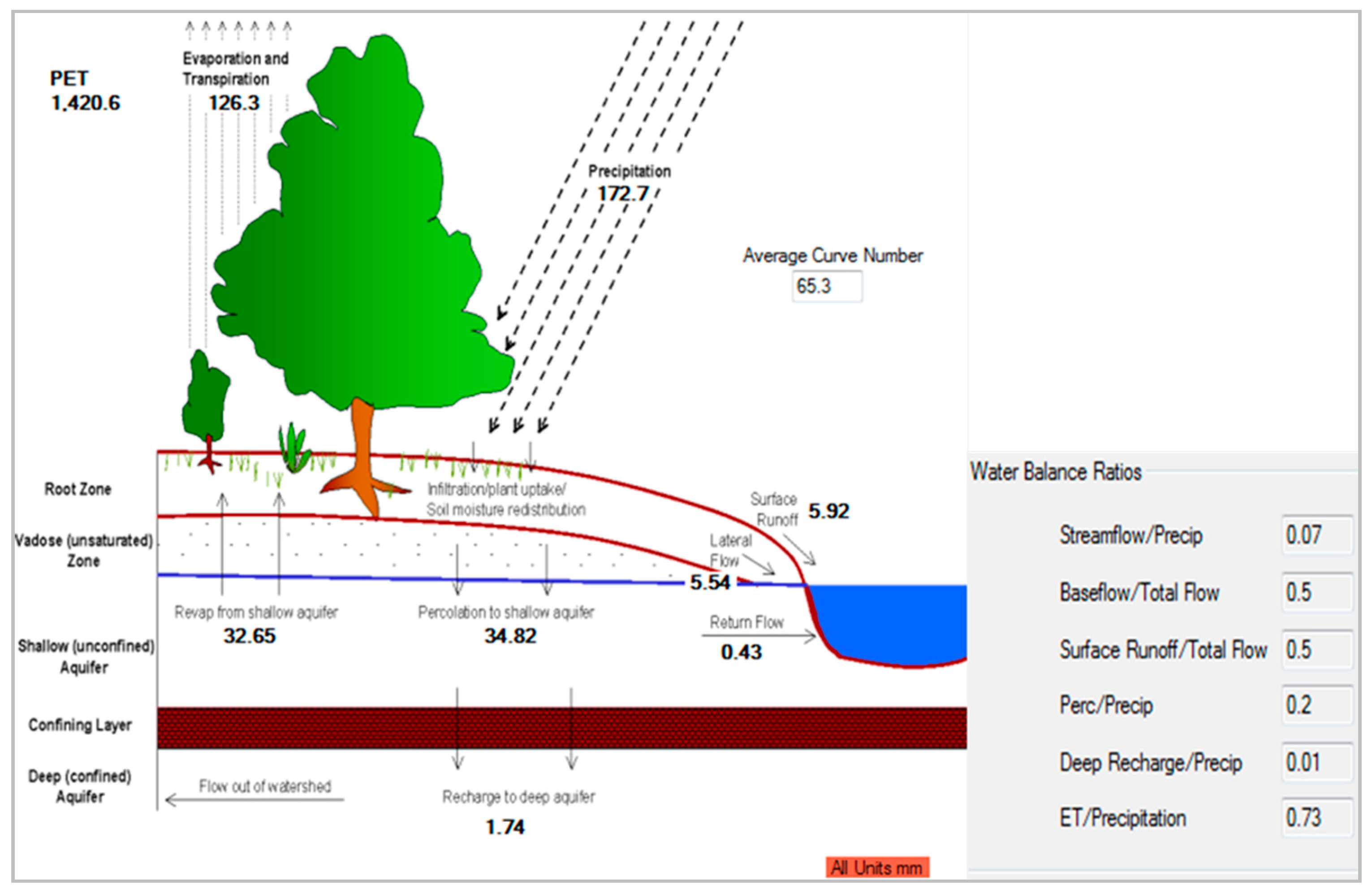
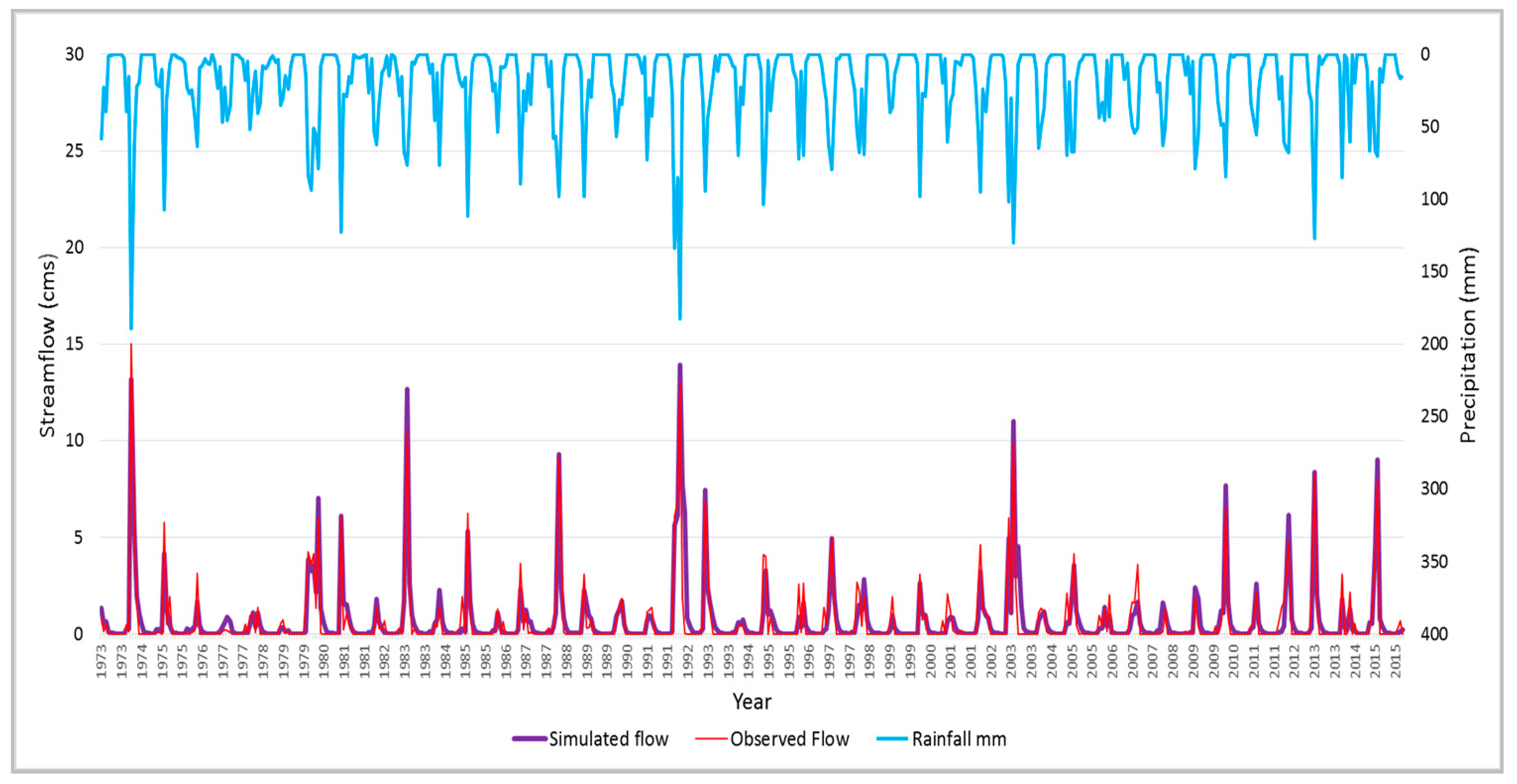
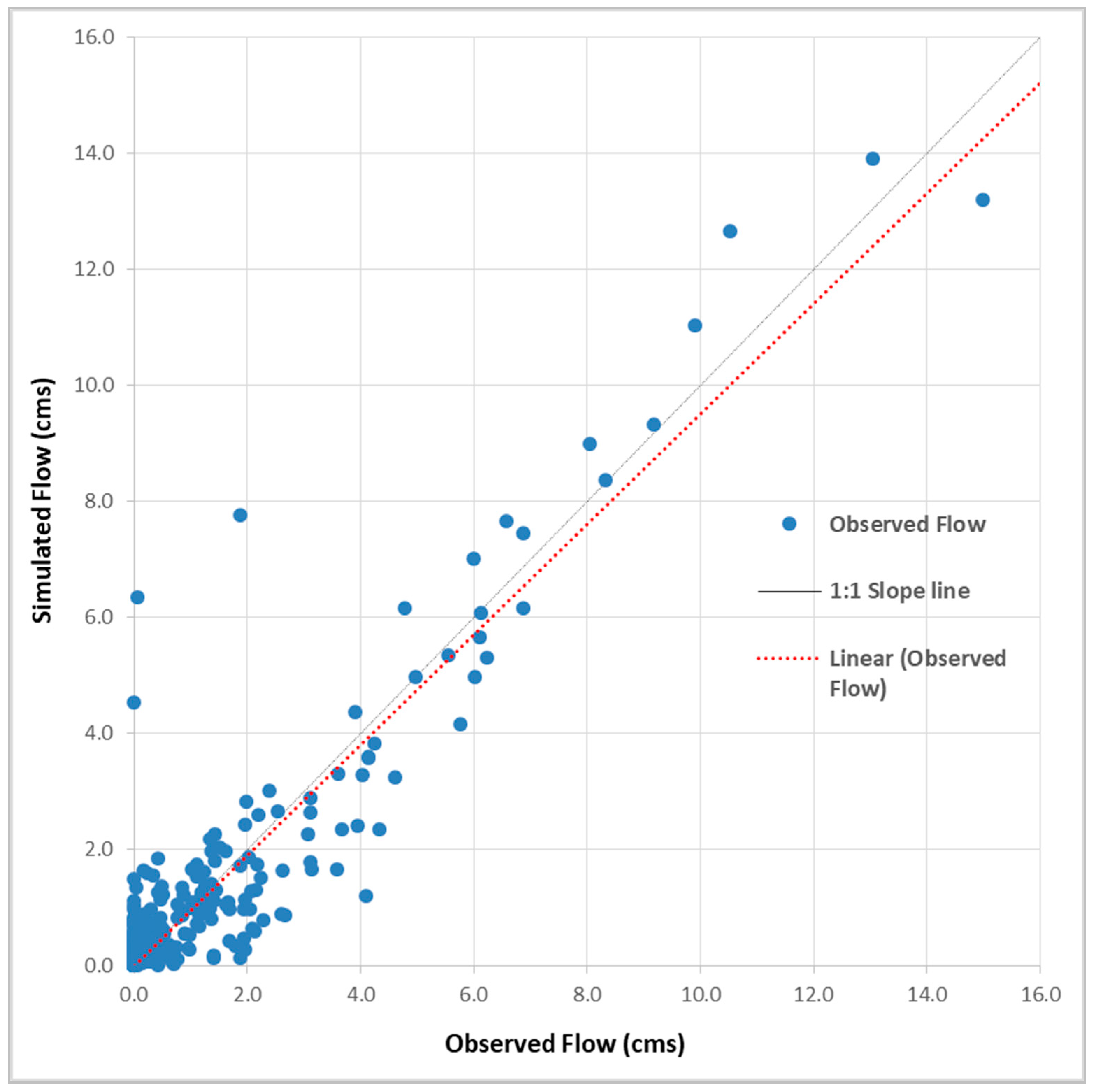
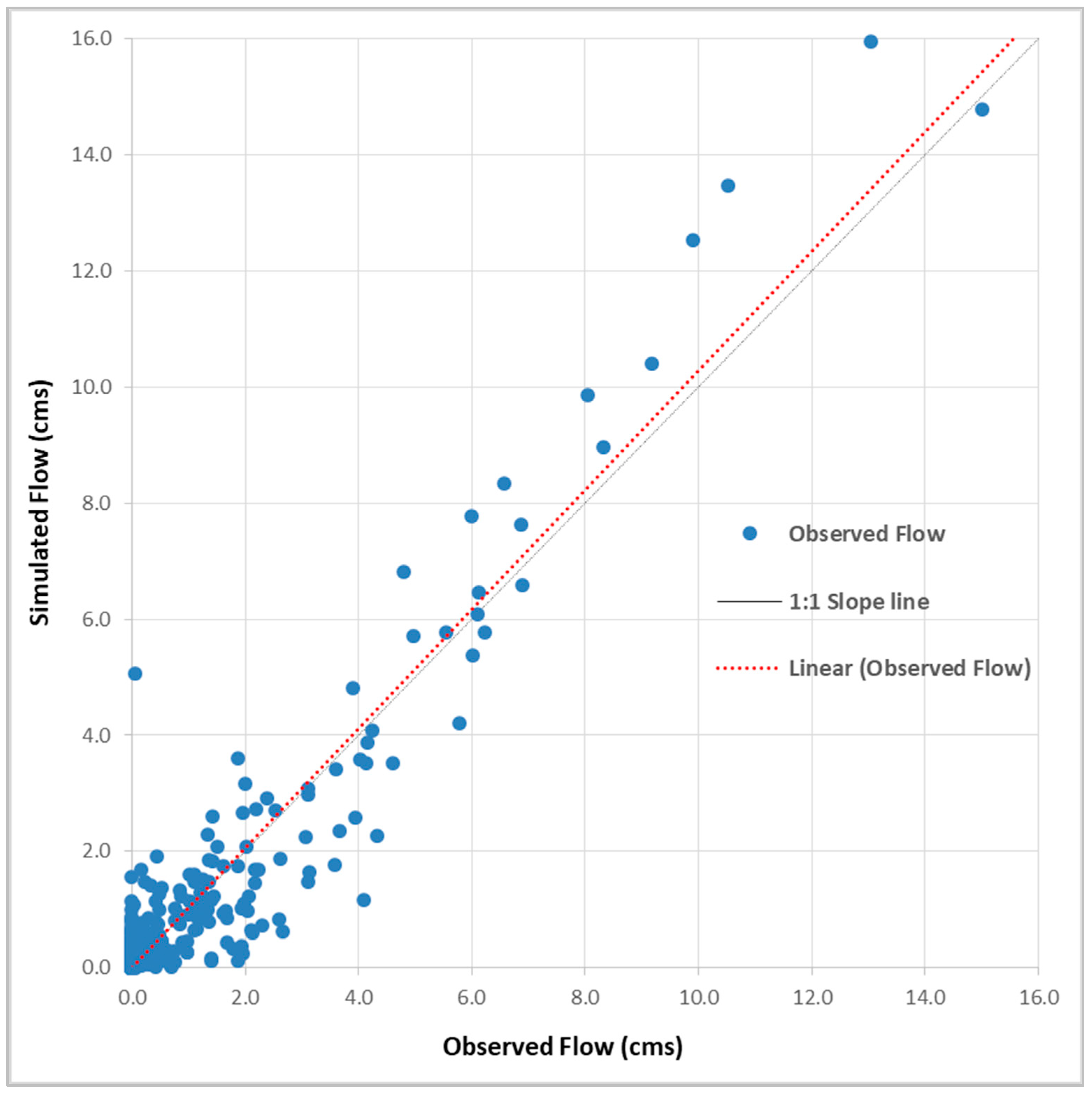
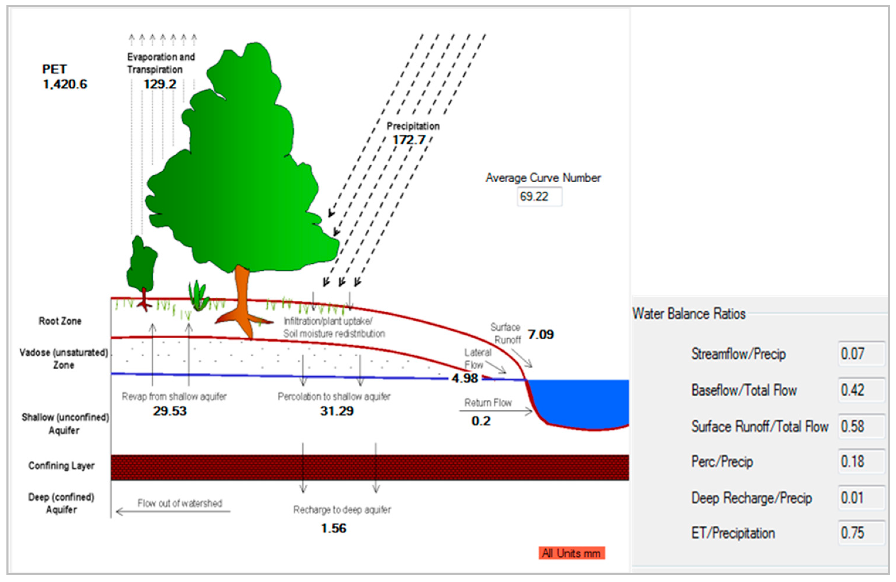
3.1. Reference Scenario
3.2. Future Scenarios
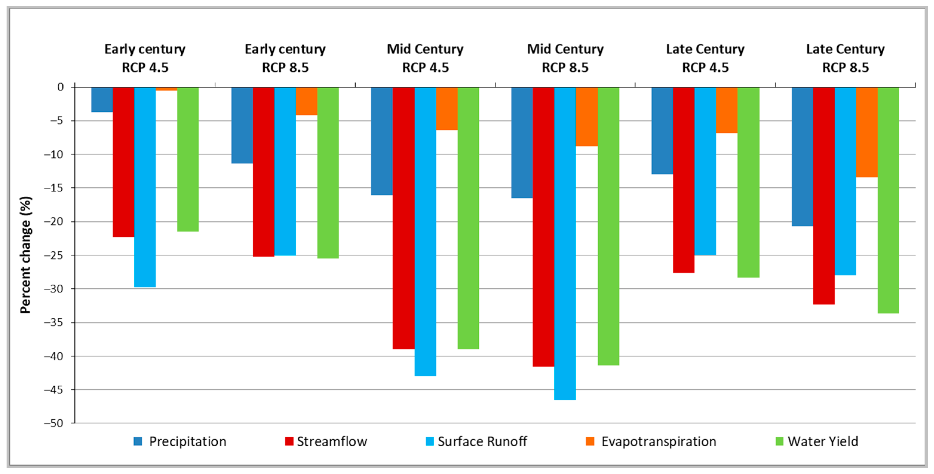
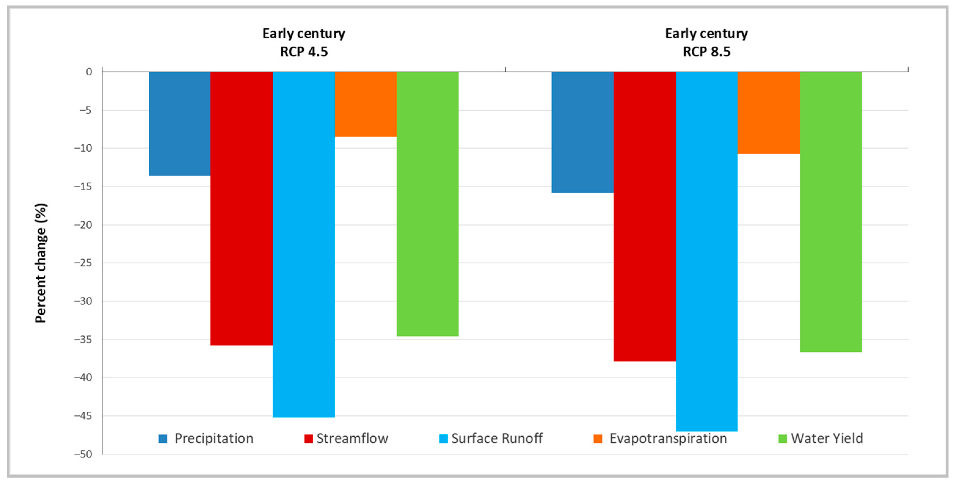
3.3. Climate Change Impacts on Surface Water Resources
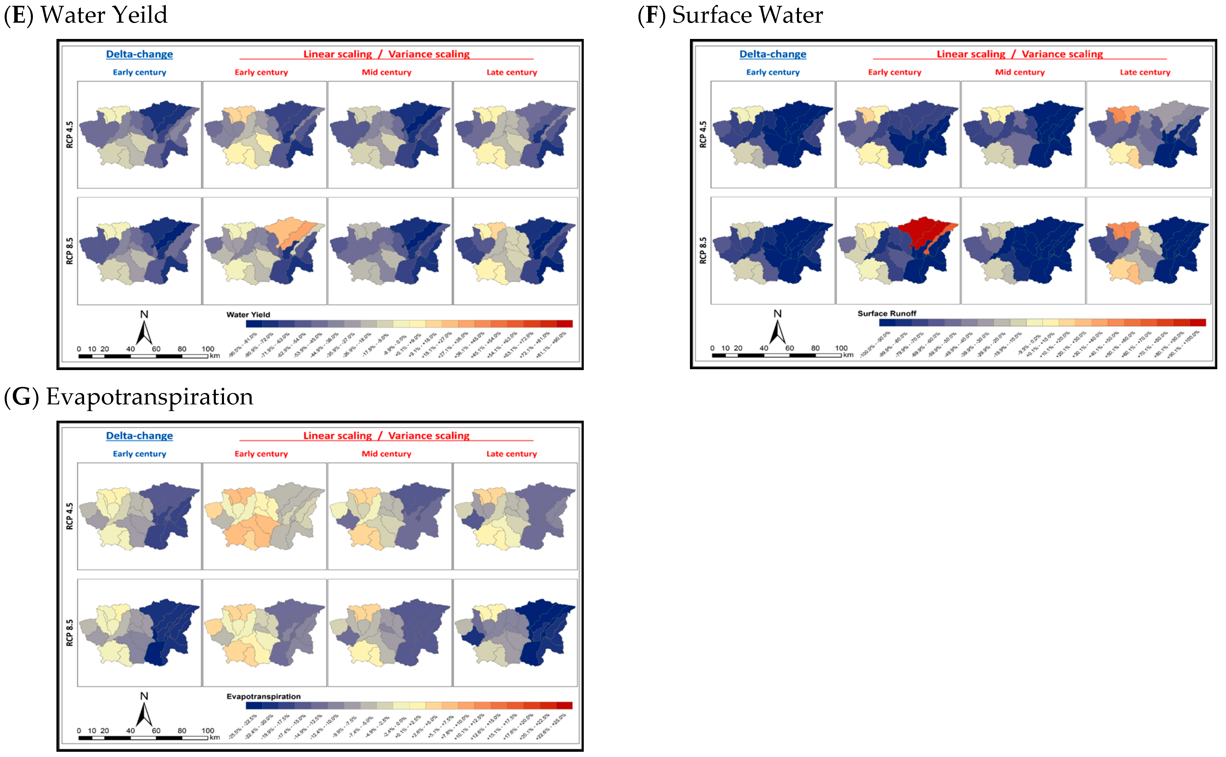
3.3.1. Temporal Changes
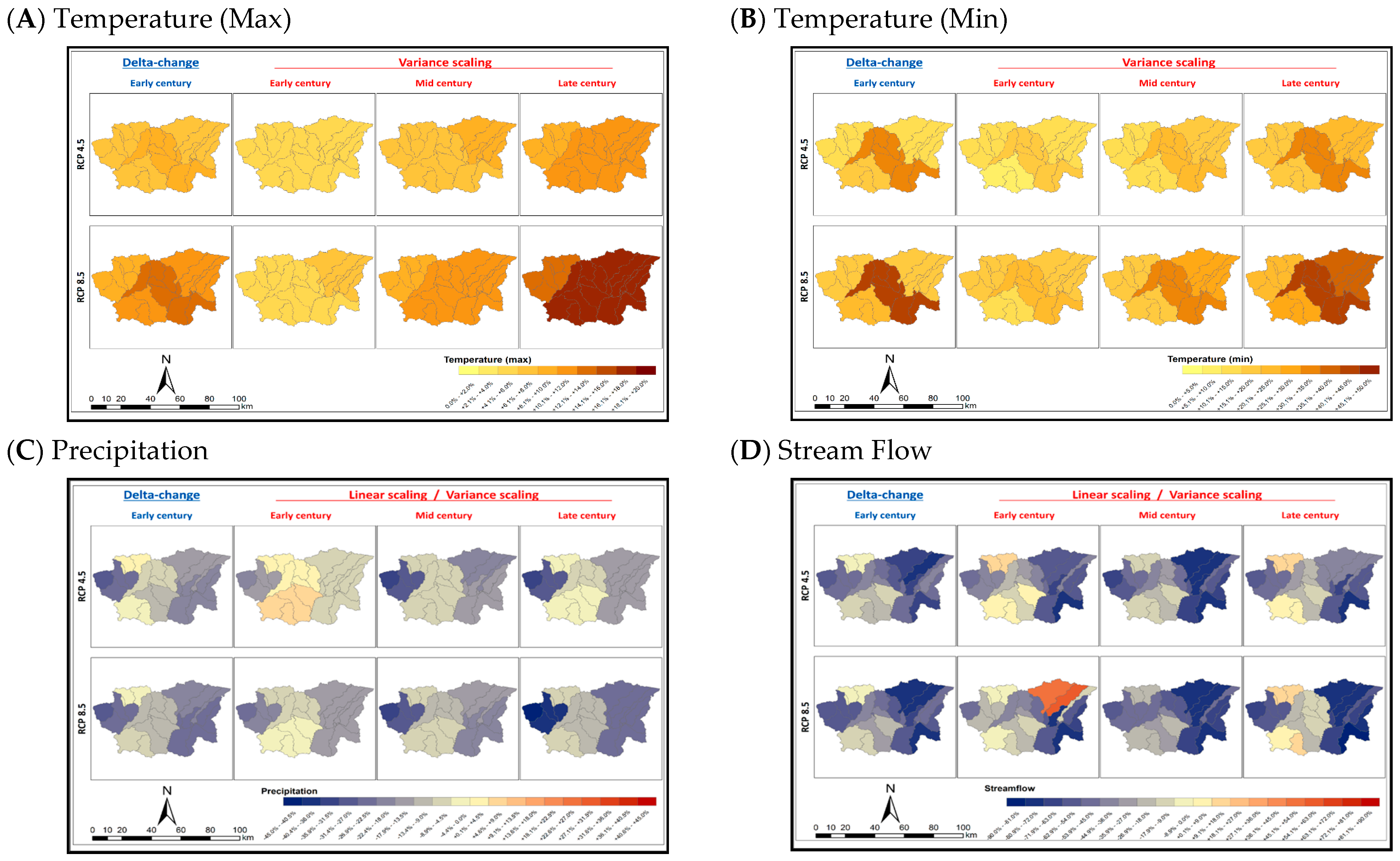
3.3.2. Spatial Changes
4. Conclusions
Supplementary Materials
Author Contributions
Funding
Data Availability Statement
Conflicts of Interest
References
- IPCC. Summary for Policymakers. In Climate Change 2021: The Physical Science Basis. Contribution of Working Group I to the Sixth Assessment Report of the Intergovernmental Panel on Climate Change; Masson-Delmotte, V., Zhai, P., Pirani, A., Connors, S.L., Péan, C., Berger, S., Caud, N., Chen, Y., Goldfarb, L., Gomis, M.I., Eds.; Cambridge University Press: Cambridge, UK; New York, NY, USA, 2021; pp. 3–32. [Google Scholar] [CrossRef]
- Sharma, J.; Ravindranath, N.H. Applying IPCC 2014 framework for hazard-specific vulnerability assessment under climate change. Environ. Res. Commun. 2019, 1, 051004. [Google Scholar] [CrossRef]
- Ministry of Environment (MOENV); United Nations Development Programme (UNDP). Jordan’s Third National Communication on Climate Change; Ministry of Environment: Amman, Jordan, 2014.
- Kour, R.; Patel, N.; Krishna, A.P. Climate and hydrological models to assess the impact of climate change on hydrological regime: A review. Arab. J. Geosci. 2016, 9, 1–31. [Google Scholar] [CrossRef]
- Flato, G.; Marotzke, J.; Abiodun, B.; Braconnot, P.; Chou, S.C.; Collins, W.; Cox, P.; Driouech, F.; Emori, S.; Eyring, V.; et al. Climate change 2013: The physical science basis. In Contribution of Working Group I to the Fifth Assessment Report of the Intergovernmental Panel on Climate Change; Cambridge University Press: Cambridge, UK, 2014; pp. 741–866. [Google Scholar]
- Trzaska, S.; Schnarr, E. A Review of Downscaling Methods for Climate Change Projections. In African and Latin American Resilience to Climate Change (ARCC); USAID: Washington, DC, USA, 2014. [Google Scholar]
- Jajarmizad, M.; Harun, S.; Salarpour, M. A Review on Theoretical Consideration and Types of Models in Hydrology. J. Environ. Sci. Technol. 2012, 5, 249–261. [Google Scholar] [CrossRef] [Green Version]
- Devia, G.K.; Ganasri, B.; Dwarakish, G. A Review on Hydrological Models. Aquat. Procedia 2015, 4, 1001–1007. [Google Scholar] [CrossRef]
- Arnold, J.G.; Kiniry, J.R.; Srinivasan, R.; Williams, J.R.; Haney, E.B.; Neitsch, S.L. Soil and Water Assessment Tool, Input/Output Documentation Version 2012. Texas Water Resources Institute TR-439. sn. 2012. Available online: https://swat.tamu.edu/media/69296/swat-io-documentation-2012.pdf (accessed on 1 January 2018).
- al Mahamid, J. Integration of Water Resources of the Upper Aquifer in Amman-Zarqa Basin Based on Mathematical Modeling and GIS. Ph.D. Thesis, Institut für Geologie, Bern, Switzerland, 2005. [Google Scholar]
- Wolff, H.P.; Al-Karablieh, E.; Al-Assa’D, T.; Subah, A.; Salman, A. Jordan water demand management study: On behalf of the Jordanian Ministry of Water and Irrigation in cooperation with the French Development Agency (AFD). Water Supply 2012, 12, 38–44. [Google Scholar] [CrossRef]
- Winchell, M.; Srinivasan, R.; di Luzio, M.; Arnold, J. ArcSWAT Interface For SWAT2012, User’s Guide; Texas Agricultural Experiment Station and Agricultural Research Service—United State Department of Agriculture: Temple, CA, USA, 2013.
- Monteith, J.L. Evaporation and environment. In Symposia of the Society for Experimental Biology; Cambridge University Press: Cambridge, UK, 1965; Volume 19, pp. 205–234. [Google Scholar]
- Soil Conservation Service (SCS). National Engineering Handbook, Section 4: Hydrology; Department of Agriculture: Washington, DC, USA, 1972; 762p.
- Williams, J.R. Flood Routing with Variable Travel Time or Variable Storage Coefficients. Trans. ASAE 1969, 12, 0100–0103. [Google Scholar] [CrossRef]
- Abbaspour, K.C.; Vaghefi, S.A.; Srinivasan, R. A Guideline for Successful Calibration and Uncertainty Analysis for Soil and Water Assessment: A Review of Papers from the 2016 International SWAT Conference. Water 2017, 10, 6. [Google Scholar] [CrossRef] [Green Version]
- Al-Qaisi, B.M. Climate Change Effects on Water Resources in Amman Zarqa Basin-Jordan; Individual Project Report for Climate Change Mitigation and Adaptation; MWI: Amman, Jordan, 2010. [Google Scholar]
- Abbaspour, K.C.; Rouholahnejad, E.; Vaghefi, S.; Srinivasan, R.; Yang, H.; Kløve, B. A continental-scale hydrology and water quality model for Europe: Calibration and uncertainty of a high-resolution large-scale SWAT model. J. Hydrol. 2015, 524, 733–752. [Google Scholar] [CrossRef] [Green Version]
- Khoi, D.N.; Thom, V. Impacts of Climate Variability and Land-Use Change on Hydrology in the Period 1981–2009 in the Central Highlands of Vietnam. Glob. NEST J. 2015, 17, 870–881. [Google Scholar] [CrossRef]
- Sunde, M.G.; He, H.S.; Hubbart, J.A.; Urban, M.A. Integrating downscaled CMIP5 data with a physically based hydrologic model to estimate potential climate change impacts on streamflow processes in a mixed-use watershed. Hydrol. Process. 2017, 31, 1790–1803. [Google Scholar] [CrossRef]
- Abbaspour, K.C. SWAT-CUP: SWAT Calibration and Uncertainty Programs—A User Manual; Eawag: Dübendorf, Switzerland, 2015; pp. 16–70. [Google Scholar]
- Abbaspour, K.C.; Vejdani, M.; Haghighat, S.; Yang, J. SWAT-CUP calibration and uncertainty programs for SWAT. In Proceedings of the Modsim 2007: International Congress on Modelling and Simulation, Christchurch, New Zealand, 10–13 December 2007; pp. 1596–1602. [Google Scholar]
- Moriasi, D.N.; Arnold, J.G.; van Liew, M.W.; Bingner, R.L.; Harmel, R.D.; Veith, T.L. Model evaluation guidelines for systematic quantification of accuracy in watershed simulations. Trans. ASABE 2007, 50, 885–900. [Google Scholar] [CrossRef]
- Gupta, H.V.; Sorooshian, S.; Yapo, P.O. Status of Automatic Calibration for Hydrologic Models: Comparison with Multilevel Expert Calibration. J. Hydrol. Eng. 1999, 4, 135–143. [Google Scholar] [CrossRef]
- The Earth System Grid Federation-ESGF Datanode. Available online: https://esg-dn1.nsc.liu.se/search/cordex/ (accessed on 20 December 2017).
- Lafon, T.; Dadson, S.; Buys, G.; Prudhomme, C. Bias correction of daily precipitation simulated by a regional climate model: A comparison of methods. Int. J. Clim. 2012, 33, 1367–1381. [Google Scholar] [CrossRef] [Green Version]
- Teutschbein, C.; Seibert, J. Bias correction of regional climate model simulations for hydrological climate-change impact studies: Review and evaluation of different methods. J. Hydrol. 2012, 456, 12–29. [Google Scholar] [CrossRef]
- Brouziyne, Y.; Abouabdillah, A.; Bouabid, R.; Benaabidate, L.; Oueslati, O. SWAT manual calibration and parameters sensitivity analysis in a semi-arid watershed in North-western Morocco. Arab. J. Geosci. 2017, 10, 427. [Google Scholar] [CrossRef]
- Whittaker, G.; Confesor, R., Jr.; Di Luzio, M.; Arnold, J.G.; Oemler, J.A. Detection of Overparameterization and Overfitting in an Automatic Calibration of SWAT. Trans. ASABE 2010, 53, 1487–1499. [Google Scholar] [CrossRef]
- American Society for Agricultural and Biological Engineering-ASABE. Guidelines for Calibration, Validation, and Evaluating Hydrologic and Water Quality Models; Approved Standard & Engineering Practice: St. Joseph, MI, USA, 2017. [Google Scholar]
- Zhang, D.; Chen, X.; Yao, H.; Lin, B. Improved calibration scheme of SWAT by separating wet and dry seasons. Ecol. Model. 2015, 301, 54–61. [Google Scholar]
- Rouholahnejad, E.; Abbaspour, K.; Vejdani, M.; Srinivasan, R.; Schulin, R.; Lehmann, A. A parallelization framework for calibration of hydrological models. Environ. Model. Softw. 2012, 31, 28–36. [Google Scholar] [CrossRef]
- Hamdi, R.; Termonia, P.; Baguis, P. Effects of urbanization and climate change on surface runoff of the Brussels Capital Region: A case study using an urban soil-vegetation-atmosphere-transfer model. Int. J. Clim. 2010, 31, 1959–1974. [Google Scholar] [CrossRef]
- Rajsekhar, D.; Gorelick, S.M. Increasing drought in Jordan: Climate change and cascading Syrian land-use impacts on reducing transboundary flow. Sci. Adv. 2017, 3, e1700581. [Google Scholar] [CrossRef] [PubMed] [Green Version]


| Data Set | Details | Source | Figure |
|---|---|---|---|
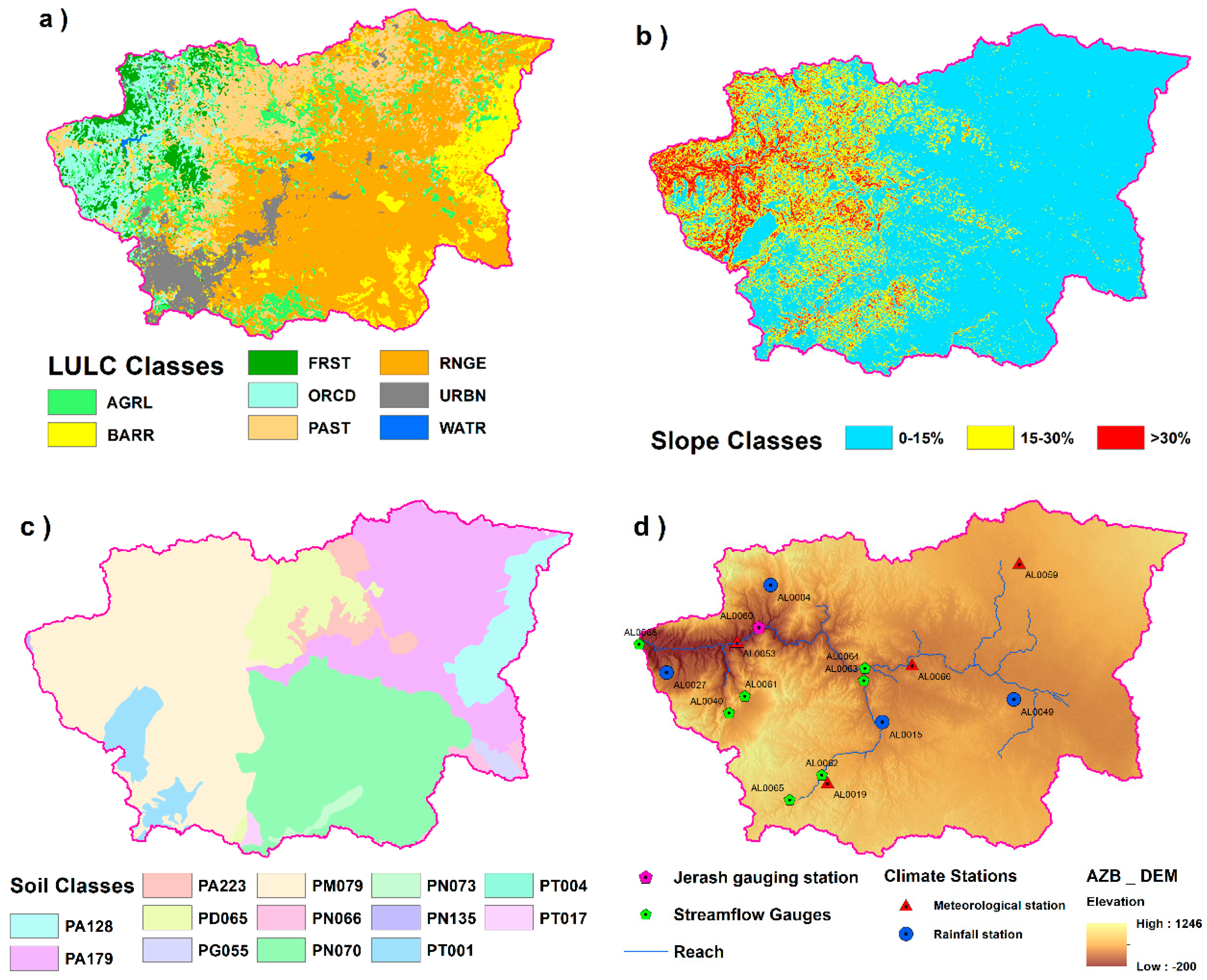
| Land use/land cover | USGS LULC classifications level 1 | Ministry of Water and Irrigation, Jordan | Figure 2a |
| Topographic Data | Shuttle Radar Topography Mission (SRTM)-30 m | USGS Earth Explorer | Figure 2b |
| Soil Map Units | Level 1 National Soil Map and Land-use Project of Jordan | Ministry of Agriculture | Figure 2c |
| Weather Dataset | Precipitation, maximum and minimum air temperature, solar radiation, wind speed, and relative humidity | Ministry of Water and Irrigation, Jordan | Figure 2d |
| Streamflow | Observed streamflow data | Ministry of Water and Irrigation, Jordan | Figure 2d |
| Parameter | Input File Type | Description |
|---|---|---|
| ESCO | Basin | Soil evaporation compensation factor |
| SURLAG | Basin | Surface runoff lag coefficient |
| EPCO | Basin | Plant uptake compensation factor |
| SOL_K | Soil | Saturated hydraulic conductivity (mm/hr) |
| SOL_AWC | Soil | Available water capacity of the soil layer ((mm H2O/mm Soil) |
| SOL_BD | Soil | Moist bulk density (g/cm3) |
| SOL_ALB | Soil | Moist soil albedo (%) |
| GW_REVAP | Groundwater | Groundwater “revap” coefficient |
| REVAPMN | Groundwater | Threshold water depth in the shallow aquifer for “revap” to occur (mm) |
| ALPHA_BF | Groundwater | Baseflow alpha factor (days) |
| GW_DELAY | Groundwater | Groundwater delay (days) |
| GWQMN | Groundwater | Threshold depth of water in the shallow aquifer required for return flow to occur (mm) |
| CANMX | HRU | Maximum canopy storage (mm H2O) |
| OV_N | HRU | Manning’s “n” value for overland flow |
| CH_K2 | Main channel | Effective hydraulic conductivity in main channel alluvium (mm/h) |
| CN2 | Management | SCS runoff curve number for moisture condition II |
| Parameter | Parameter Range | Initial Value | Change Type | Initial Range | Fitting Value | Calibrated Value | ||
|---|---|---|---|---|---|---|---|---|
| Min | Max | Min | Max | |||||
| CN2 * | 35 | 98 | 65.3 | Additive | −5 | 5 | 4.02 | 69.22 |
| SOL_K * | 0 | 2000 | 7.35 | Relative | −0.8 | 0.8 | −0.16 | 6.17 |
| SOL_AWC * | 0 | 1 | 0.106 | Relative | −0.5 | 0.5 | 0.13 | 0.12 |
| ESCO | 0 | 1 | 0.01 | Additive | 0 | 0.2 | 0.007 | 0.02 |
| SURLAG | 0.05 | 24 | 1 | Replace | 0.2 | 3 | 1.8 | 1.8 |
| GW_DELAY | 0 | 500 | 31 | Replace | 10 | 31 | 40.28 | 40.28 |
| Objective Function | Calibration Period (1973–2002) | Validation Period (2003–2015) |
|---|---|---|
| R2 | 0.9 | 0.81 |
| NSE | 0.89 | 0.86 |
| PBIAS | −6.3 | 0.9 |
| RSR | 0.34 | 0.39 |
| Mean_sim (Mean_obs) | 0.71 (0.67) | 0.64 (0.64) |
| StdDev_sim (StdDev_obs) | 1.83 (1.75) | 1.70 (1.53) |
| Variable (Daily) | Bias Correction Method | RMSE (1:1 Fit Line) * | R2 ** |
|---|---|---|---|
| Precipitation (mm) | Linear scaling | 4.647 | 0.004 |
| Local intensity scaling | 4.667 | 0.0039 | |
| Distribution mapping | 4.751 | 0.0034 | |
| Power transformation | 4.866 | 0.0033 | |
| Minimum Temperature (°C) | Variance scaling | 3.846 | 0.667 |
| Distribution mapping | 3.881 | 0.662 | |
| Linear scaling | 4.235 | 0.619 | |
| Maximum Temperature (°C) | Distribution mapping | 5.359 | 0.624 |
| Variance scaling | 5.417 | 0.617 | |
| Linear scaling | 5.42 | 0.618 |
| RCP | Climate Variable | Reference Period | Delta-Change | linear Scaling/Variance Scaling | ||||||
|---|---|---|---|---|---|---|---|---|---|---|
| EC | ∆ | EC | ∆ | MC | ∆ | LC | ∆ | |||
| RCP 4.5 | PCP | 221.6 | 197.4 | −24.2 | 206.8 | −14.7 | 178.9 | −42.6 | 185.5 | −36.1 |
| TMP max | 25.5 | 27.5 | 2.1 | 26.7 | 1.3 | 27.3 | 1.9 | 28.2 | 2.7 | |
| TMP min | 11.4 | 13.5 | 2.1 | 12.8 | 1.4 | 13.4 | 2.0 | 13.9 | 2.5 | |
| RCP 8.5 | PCP | 221.6 | 193.3 | −28.3 | 201.6 | −20.0 | 187.4 | −34.2 | 177.0 | −44.6 |
| TMP max | 25.5 | 28.3 | 2.8 | 26.9 | 1.5 | 28.2 | 2.7 | 29.4 | 4.0 | |
| TMP min | 11.4 | 14.2 | 2.8 | 13.3 | 1.8 | 14.1 | 2.7 | 15.1 | 3.7 | |
| RCP | Water Balance Component | Reference Period | Delta-Change | Linear Scaling/Variance Scaling | ||||||
|---|---|---|---|---|---|---|---|---|---|---|
| Early-Century | ∆ | Early-Century | ∆ | Mid-Century | ∆ | Late-Century | ∆ | |||
| RCP 4.5 | Precipitation | 172.7 | 149.2 | −23.5 | 166.3 | −6.4 | 145.0 | −27.8 | 150.4 | −22.3 |
| Streamflow | 12.3 | 7.9 | −4.4 | 9.5 | −2.7 | 7.5 | −4.8 | 8.9 | −3.4 | |
| Surface Runoff | 7.1 | 3.9 | −3.2 | 5.0 | −2.1 | 4.0 | −3.0 | 5.3 | −1.8 | |
| Evapotranspiration | 129.2 | 118.2 | −11.0 | 128.5 | −0.7 | 121.0 | −8.2 | 120.4 | −8.8 | |
| Water Yield | 13.8 | 9.1 | −4.8 | 10.9 | −3.0 | 8.4 | −5.4 | 9.9 | −3.9 | |
| RCP 8.5 | Precipitation | 172.7 | 145.3 | −27.4 | 153.1 | −19.6 | 144.3 | −28.5 | 137.0 | −35.7 |
| Streamflow | 12.3 | 7.6 | −4.6 | 9.2 | −3.1 | 7.2 | −5.1 | 8.3 | −4.0 | |
| Surface Runoff | 7.1 | 3.8 | −3.3 | 5.3 | −1.8 | 3.8 | −3.3 | 5.1 | −2.0 | |
| Evapotranspiration | 129.2 | 115.4 | −13.8 | 123.8 | −5.4 | 117.8 | −11.4 | 111.9 | −17.3 | |
| Water Yield | 13.8 | 8.8 | −5.1 | 10.3 | −3.5 | 8.1 | −5.7 | 9.2 | −4.7 | |
Disclaimer/Publisher’s Note: The statements, opinions and data contained in all publications are solely those of the individual author(s) and contributor(s) and not of MDPI and/or the editor(s). MDPI and/or the editor(s) disclaim responsibility for any injury to people or property resulting from any ideas, methods, instructions or products referred to in the content. |
© 2023 by the authors. Licensee MDPI, Basel, Switzerland. This article is an open access article distributed under the terms and conditions of the Creative Commons Attribution (CC BY) license (https://creativecommons.org/licenses/by/4.0/).
Share and Cite
Al-Hasani, I.; Al-Qinna, M.; Hammouri, N.A. Potential Impacts of Climate Change on Surface Water Resources in Arid Regions Using Downscaled Regional Circulation Model and Soil Water Assessment Tool, a Case Study of Amman-Zerqa Basin, Jordan. Climate 2023, 11, 51. https://doi.org/10.3390/cli11030051
Al-Hasani I, Al-Qinna M, Hammouri NA. Potential Impacts of Climate Change on Surface Water Resources in Arid Regions Using Downscaled Regional Circulation Model and Soil Water Assessment Tool, a Case Study of Amman-Zerqa Basin, Jordan. Climate. 2023; 11(3):51. https://doi.org/10.3390/cli11030051
Chicago/Turabian StyleAl-Hasani, Ibrahim, Mohammed Al-Qinna, and Nezar Atalla Hammouri. 2023. "Potential Impacts of Climate Change on Surface Water Resources in Arid Regions Using Downscaled Regional Circulation Model and Soil Water Assessment Tool, a Case Study of Amman-Zerqa Basin, Jordan" Climate 11, no. 3: 51. https://doi.org/10.3390/cli11030051