1. Introduction
The forecast of populations in low-elevation coastal areas began at more than 680 million people in 2010 and will possibly exceed 1000 million by 2041–2060 [
1]. As global temperatures rise, rising sea levels will threaten the lives and property of societies in coastal regions, creating economic, social, and environmental problems and increasing the frequency and intensity of coastal flooding [
2]. Therefore, it is essential to estimate sea level rise by the end of this century under different global warming conditions.
The average sea level increased 20 cm between 1901 and 2018, with an annual average of 1.3 mm between 1901 and 1971, increasing to 1.9 mm between 1971 and 2006 and 3.7 mm between 2006 and 2018. Human influence is the most likely cause of such increases [
3]. The Paris Agreement proposed limiting future temperature increase to 1.5 °C compared to the second half of the nineteenth century so as to reduce the impacts of climate change [
4]. Since the Fourth Assessment Report (AR4) of the Intergovernmental Panel on Climate Change (IPCC), progress has been made in observing the average changes in sea level and the different components that contribute to it [
1,
3,
5]. Total sea level rise is about 3 mm per year (about one-eighth of an inch per year). About one-third comes from Greenland and Antarctica, one-third from glaciers, and one-third from the expansion of seawater as it warms [
6,
7].
Long-term models have sparked debate about the possibility of future sea level increases that are more significant than the IPCC’s projections [
3,
5,
8,
9]. Policymakers, planners, coastal engineers, and civil society need clear sea level rise projections for risk assessment and decision making [
10]. The problem is more complex if it is addressed at the regional level:
“Regional Relative Sea Level = Short-Term Effects + Sterodynamic Variability + Glaciers + Land Water Storage + Ice Sheets + Subsidence” [
11]. The absence of this type of projection at the regional level has meant an evident lack of concern about the problem of climate change in local governments, which has been detected by civil actors trying to influence political agenda in this regard [
12].
Studies predicting the contribution of the Antarctic ice sheet to sea level rise show that by 2081–2100 [
13], the sum of the components of global sea level rise will exceed 1.5 m. According to Mastrandrea et al. (2011), the level of confidence assigned to research depends on the line of evidence that provides information for research and its degree of consistency [
14]. Hinkel et al. (2019) state that coastal communities need to understand the expected changes in the height and frequency of extreme sea level events (ESL) in order to select appropriate and cost-effective adaptation strategies [
10]. Medium-term decisions (30 years) include flood control and other infrastructure and spatial planning decisions.
Coastal protection infrastructure, such as levees and breakwaters, involves making decisions that span 30 to 100 years or even longer [
15]. Critical protective infrastructure, such as wind barriers, requires decades of planning and implementation, so its lifespan must be even longer [
16]. That is, in this sector of decision making, horizons of more than 100 years must be considered if a long-term critical infrastructure is planned [
17]. Land-use planning, coastal zone risk zoning, and coastal adjustment decisions [
18] should be considered to last as long as a century. Representative Concentration Pathways (RCPs) describe different levels of greenhouse gases (GHGs) and other radiative emissions that could occur in the future. The four pathways encompass a wide range of climate system forcings between 2081 and 2100—2.6, 4.5, 6.0, and 8.5 watts per square meter (W/m
2)—but these are not accompanied by any socioeconomic “narrative” [
19,
20].
Socioeconomic factors that will be relevant over the next century include population, economic growth, education, urbanization, and the pace of technological development [
21]. The Shared Socioeconomic Pathways (SSPs) examine five ways in which the world would evolve in the absence of climate policies and how different levels of climate change mitigation could be achieved when the mitigation objectives of the RCPs are combined with the SSPs [
22]. Both routes are complementary. The RCPs set the trajectories of the greenhouse gas concentrations and the magnitudes of radiative forcings that could occur by the end of the century; the SSPs establish the context in which emission reductions will (or will not) be achieved [
23], particularly in coastal zones.
The preceding studies have shown the need to display data that is under large uncertainties, both with respect to the understanding of climate change and as a tool for decision makers [
24], particularly in coastal zones. Over the past four decades, elevation, specifically Digital Elevation Models (DEMs), have been used to identify low-lying coastal areas [
25,
26,
27]. Previous research has shown that the quality of the data, and the transformations to which they are subjected, influence the correct modeling of future impacts [
28,
29,
30].
The present work aimed to use recent satellite images to extract a digital elevation model of the study area through the sea level projections of Kopp et al. (2017) and the flood probability statistics of Muis et al. (2016). Three different coastal flood scenarios were generated: SSP1-RCP2.6 for the sustainable pathways, SSP2-RCP4.5 for moderate commitment, and SSP5-RCP8.5 for fossil fuel-rich development [
31,
32].
This work is based on the fact that Mexico in general, and Acapulco in particular, is following a pathway that is not committed to future economic and social development [
33], with little investment in education or health at the national level, driven by an economy based on fossil fuels and high energy consumption, along with rapid growth of the population, persistent inequality, and poverty [
34,
35]. It represents a heterogeneous state with a continuously increasing population and a plan of economic growth oriented towards mass tourism, which is more fragmented and slow than in other areas [
36].
Study Area
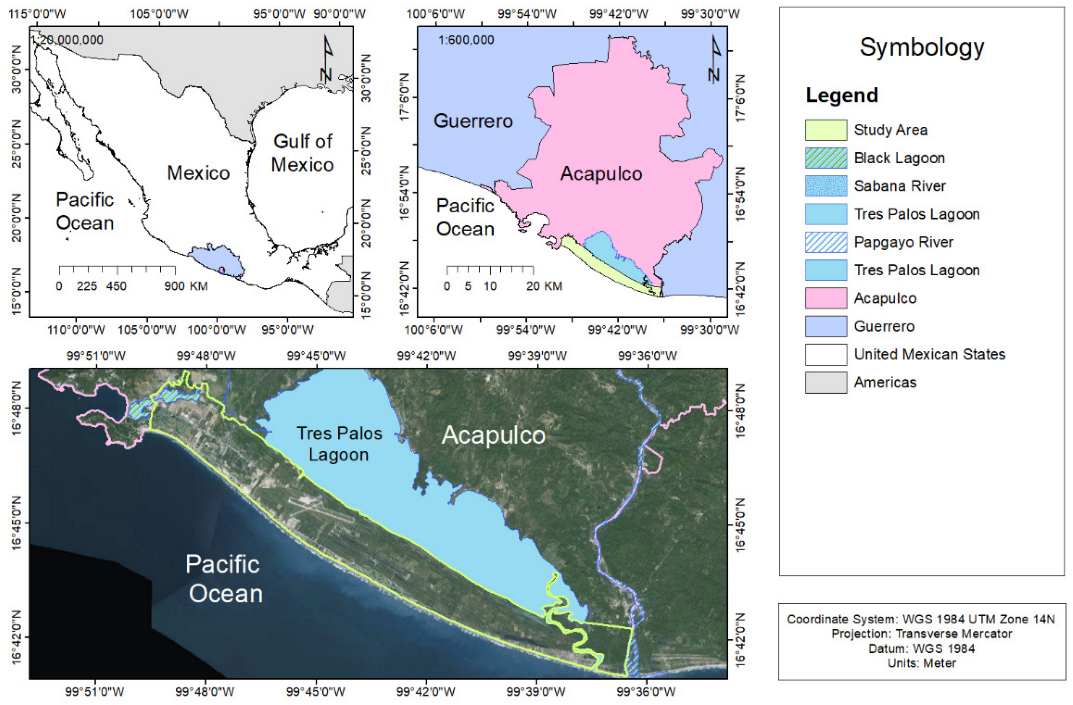
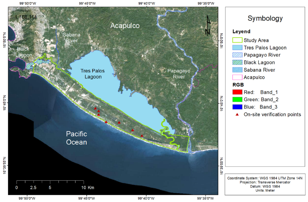
Acapulco is a Mexican city and port located in the state of Guerrero, on the south coast of the country, 379 km by road from Mexico City [
37]. It is the largest city in the state, with 658,609 inhabitants, and is the municipality with the largest population, with 779,566 denizens [
38]. The general location of Acapulco within the Mexican Republic, and the location of the study area, are shown in
Figure 1.
Acapulco is one of Mexico’s top tourist destinations [
39]. It has a coastline approximately 62 km long (12.3% of the coast of the state of Guerrero), and it exhibits a high level of environmental deterioration. From 2010 to 2015, the state of Guerrero lost 17.8% of its mangrove areas, equivalent to 1448 ha [
40]. In 1921, the municipality of Acapulco was inhabited by 5768 people; by 1950, there were 55,892 inhabitants [
41]; by 2010, there were 789,971 [
42]; and the 2020 census recorded a population of 779,566 inhabitants, that is, about 10,000 inhabitants fewer than a decade earlier.
The city comprises three large tourist areas [
43]: Acapulco Tradicional, Acapulco Dorado, and Acapulco Diamante (
Figure 2). Each area was developed in different eras: the Acapulco Tradicional is the central area of the city and the historical point of origin of its urban environment. Acapulco Dorado was created in the 1950s, and Acapulco Diamante arose at the end of the 1980s. The geographical boundaries of the study area are specified in
Table 1. The boundaries of the study area within the Acapulco Diamante zone are shown in
Figure 1 and are as follows:
To the north, the lagoon of Tres Palos (also known as Nahualá);
To the east, the Papagayo River;
To the south, the Pacific Ocean;
To the west, the Black Lagoon.
The coastal area of the municipality of Acapulco has historically been very vulnerable to hydrometeorological phenomena [
44]. It is exposed to coastal flooding by tropical storms, as occurred with hurricane Henriette in 1995 [
45], hurricane Paulina in 1997 [
46], and hurricanes Ingrid and Manuel in 2013 [
47,
48].
Thanks to the infrastructural improvement, mainly due to the investment in tourism promotion programs in the Diamante area, the development of housing has caused a constant increase in population density in this area, which has increased the population at risk of coastal flooding [
49,
50]. Despite being one of the most valuable areas in the city, it is also a high-risk area [
51]. The Diamante Zone is home to about a quarter of the municipality’s population and comprises a quarter of the urban infrastructure [
52].
The Atlas of Natural Hazards of the City of Acapulco [
53] identifies sites with severe problems of pluvial flooding, especially towards the eastern part of the city in the areas adjacent to the Laguna de Tres Palos. Another area that has been identified is located between the Black Lagoon and the Pacific Ocean. Both areas are flat, which increases the difficulty of draining the excess water from bottlenecks of natural channels and parts of the Acapulco Diamante zone.
However, even though Acapulco is the largest city in Guerrero, it currently lacks a proposal for the reduction of risk due to sea level rise, which has been validated and endorsed by social actors [
42]. Although there have been institutional efforts to assess risk, action has not been taken [
46].
2. Materials and Methods
In this work, estimates of future sea level rise based on the climate projections constructed by Kopp et al. (2017) have been made by adding the possibility of the early decline of the West Antarctic ice sheet [
31,
54] with different ranges of future sea level rise under different climate change scenarios. We used the flood risk statistics published by Muis et al. (2016), who studied 35 years of global atmospheric condition records to simulate and estimate the frequency of extreme flooding around the world [
31,
32].
For their global sea level rise projections, Kopp et al. (2017) assume that there is independence among sea level contributors, so they use expert judgment for correlation of uncertainty in the projections, which shows that with RCP 8.5, by 2100, at the 99.5th percentile of their sea level projection, it increased from 176 cm (their uncorrelated hypothesis) to 187 cm (with the expert correlation) [
31]. This shows the effect of the correlation structure for the tail of the future sea level distribution. It is essential to broaden the range of the probabilities at stake, because low probability events are also important for risk management assessment, as long as they have a high impact [
55].
The IPCC Group 1 Sixth Assessment Report (from now on, AR6W1) provides projections of sea levels and their uncertainty [
3]. The AR6W1 projections of sea level rise are based on the following SSP-RCPs: SSP1-RCP2.6 for sustainable pathways, SSP2-RCP4.5 for a moderate commitment, and SSP5-RCP8.5 for fossil fuel-rich development. For physical reasons, the instability of the sea ice sheet, the detachment of glaciers, and the thermal expansion of the oceans all place an upper limit on sea level rise by 2081–2100 [
56]. Recent projections can be used to assess this limit. Related studies show global consensus on a projected increase of between 2 and 4 m by 2081–2100, in relation to the values pertaining to the beginning of this century [
57].
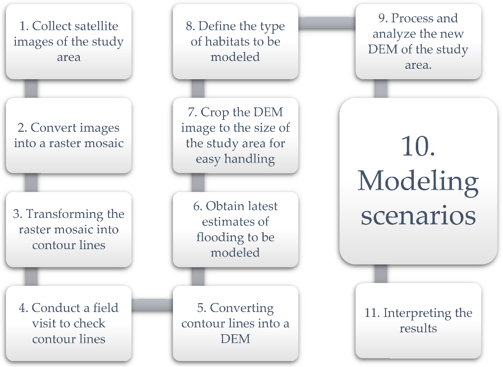
The here-presented
Integrated Procedure for Estimate Sea Level Impacts (IPESLI) integrates Landsat images, official databases, and design software for geographic information systems. IPESLI is useful in areas with little georeferenced and validated information (
Figure 2).
Table 2 presents the projected values of global warming for 2041–2060, 2061–2080, and 2081–2100, relative to the base values of 1995–2014 [
3]. Using the NASA Sea Level Projection Tool, we are able to visualize the local projection data from the IPCC 6th Assessment Report (AR6) [
58].
The IPCC’s projections of future sea level rise are derived from models based on different processes [
3]. Ocean warming causes thermal water expansion, the melting of high mountain glaciers and polar ice caps in Greenland and Antarctica, increases in the amount of groundwater extracted, and contributions of continental surface water. We believe the local projections underestimate the sea level rise in the study area; therefore, the projections used in our scenarios are based on three pairs of SSP-RCPs adapted from the climate projections constructed by Kopp et al. 2017 [
31].
The three scenarios of sea level rise employed in this paper (
Table 2) are described below.
A. Optimistic scenario: SSP1-RCP2.6 is a “rigorous” approach. According to the IPCC, SSP1-RCP2.6 requires that carbon dioxide (CO2) emissions begin to decline in 2020 and reach zero by 2081–2100, consistent with the 1.5 °C warming cap, a target of the Paris Agreement. It implies 840 gigatons of total net carbon pollution by 2081–2100.
B. Conservative scenario: SSP2-4.5 emissions will peak around 2040 and then decline to half the 2041–2060 level by 2081–2100. This implies approximately 2 °C of warming from the 1850–1900 level and 1266 gigatons of total carbon pollution by 2081–2100.
C. Extremist scenario: In SSP5-8.5, emissions continue to increase throughout the 21st century. RCP8.5 is considered the basis of the worst-case climate change scenario, and the result is an overestimation of projected coal production. This scenario is named “Extremist” in this study. It involves 3 or 4 °C of heating and 2430 gigatons of carbon dioxide equivalent emissions by 2081–2100.
Different datasets were obtained from sources such as digital images, cartography, and field data for the area of Acapulco Diamante and its coast [
59]. Cartographic information on coastal water bodies (e.g., Laguna de Tres Palos) [
60] and the outline of the coast (e.g., inner rim and coast) were obtained from the National Institute of Statistics and Geography (from now on, INEGI) [
61]. USGS Earth Explorer is a platform containing one of the largest databases of specialized information from various remote sensing satellites. A shapefile of the study area was used to define the region of interest, which is the geographic boundary that restricts the search in order to acquire data. A shapefile of the study area was delimited between 2019 and 2020. We selected L8 OLI/TIRS and L7 ETM + [
62].
Table 3 lists the extracted images, the satellite from which they were taken, and their respective dates. Spatial resolution refers to the size of a pixel on the ground. Landsat data have a 50 m resolution, meaning that each pixel represents an area of 50 m × 50 m above the ground [
59].
Once the raw images were obtained, image band analysis was done, through which the image could be organized in such a way that unique and current information could be extracted. We used the natural color compound with a combination of red (4), green (3), and blue (2) bands; see
Figure 2. This approximates what human eyes see: while healthy vegetation is green, unhealthy flora is brown. Urban features appear in white and gray, water is dark blue or black, and the combinations of bathymetric bands (4, 3, 1) use red (4) and green (3), with coastal bands peaking in the water. The coastal band is helpful in coastal, bathymetric, and aerosol studies because it reflects blues and violets.
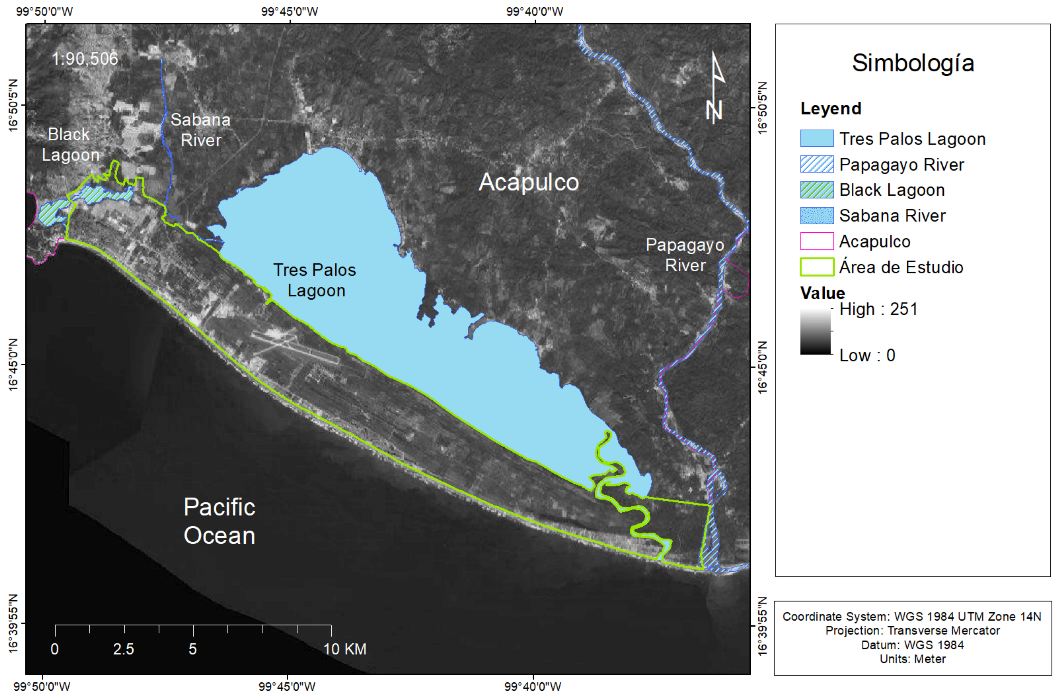
A source tile dataset was formed in ArcGIS 10.7.1 for each generated image set. A mosaic dataset was derived from managing the entire collection, and finally, the reference tile dataset was obtained to apply the final scenarios (
Figure 3). The problems of data management were concerned with merging different geographical areas and resolutions.
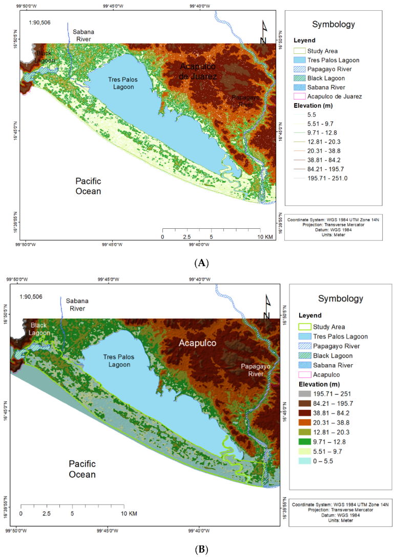
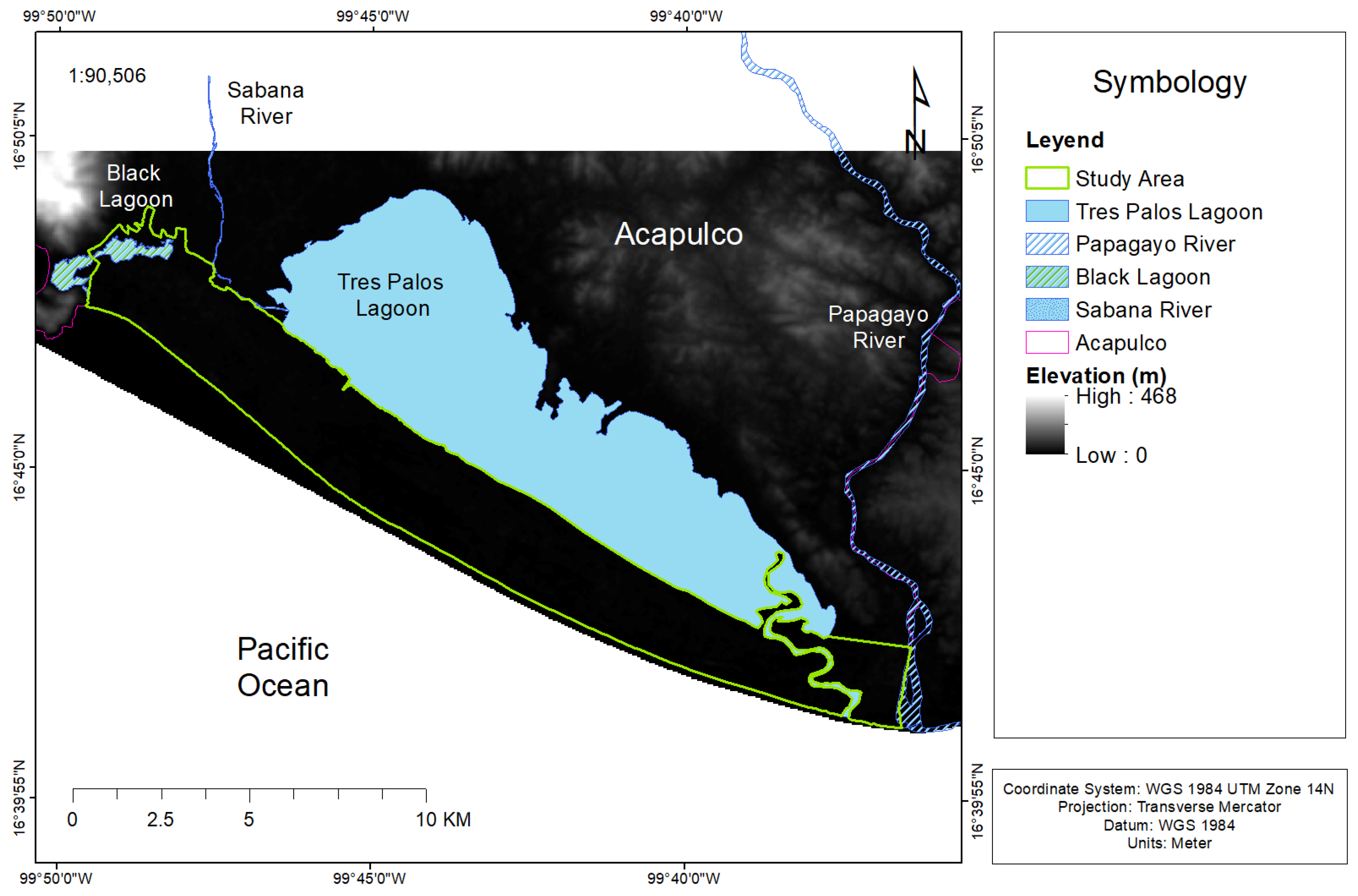
Once the mosaic data were obtained, a series of contour lines was created in Global Mapper 20 from the terrain grid. In this way, equally spaced contour lines were generated at intervals that were as small as possible from the elevation grid data entered into ArcGIS (10 cm). However, we also experimented with distances between 5 m and 1 cm, with more significant and lesser degrees of success. Next, the terrestrial LiDAR point cloud was processed on a contour map (
Figure 4A).
ArcGIS 10.7.1 used contour lines to build a triangulated irregular network (TIN). The TIN components were constructed from vector data, which represent surface features. Once the TIN was created, geoprocessing tools were used to add additional vector data, thus generating a network of streams and delineating watersheds; see
Figure 4B. In situ data were required and were collected during May 2018 and May 2019 in the Diamante Zone to validate the modeling. Through seven field visits made to different villages within the study area (
Figure 5), empirical terrain data (in situ) were obtained with GPS receivers, which allowed us to estimate a negative bias on the average vertical axis of −5.7 m.
INEGI’s cartographic maps show a resolution 4.53175 m below that obtained with our raster, which we have used as the digital elevation model. Therefore, a “manual” adjustment was made in the database; this adjustment consisted of subtracting the value of 4.53175 m from the minimum elevation value of each layer in INEGI. In the maps herein, said error was eliminated. Once the TIN was obtained with additional hydrography data, we transformed the resulting layer into a raster by interpolation. ArcGIS assigns each output cell a height, or a value without information, depending on whether the center of the cell falls within the TIN interpolation zone or not (
Figure 6). The output raster more accurately represents the TIN surface; since the raster has a cell structure, it cannot maintain the edges of the thick and thin cutting lines present in the TIN [
63].
A sensitivity analysis was applied to the resolution of the generated raster through three sets of simulations. The raster images were generated for sensitivity analysis with spatial resolutions of 10 m, 20 m, and 50 m [
63]. The bilinear interpolation method generated the images using a weighted average of the four closest cell centers. The closer the input cell to the center of the output cell, the greater the influence of its value on the value of the output cell. This means that the output value may differ from the nearest input’s, but it is always within the same range of values as the input [
64].
Once the final raster was obtained, this public image was cropped with the shapefile of the specific study area of the Diamante Zone. The horizontal resolution of the elevation data is one arcsecond, which corresponds to approximately 50 m. The maps reflect land elevations relative to extreme coastal water levels and do not incorporate potential defenses such as levees.
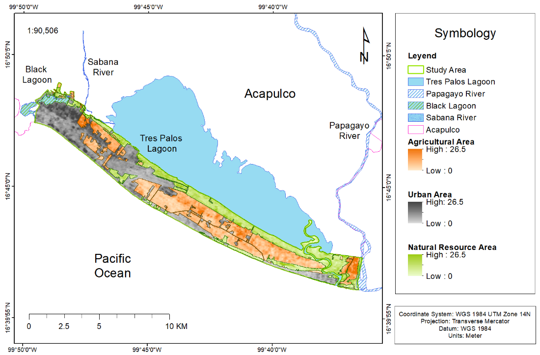
The territory of the study area was classified into three main types to assess land use (
Figure 7):
Agricultural area (cultivated land, livestock production, and aquaculture);
Urban area (residential, recreation, culture, wholesale warehouse, commercial building, business, financial services, market, and plant nursery);
Natural resource areas (bodies of water, mangrove, xerophilous scrub, and low deciduous forest).
The impacts of coastal flood risk on agricultural, urban, and natural resource areas were mapped. The impacts of flooding on each of the habitat types identified in the study area were classified into the scenarios Optimistic SSP1-RCP2.6, Conservative SSP2-RCP4.5, or Extremist SSP5-RCP8.5; see
Figure 7.
Historical observed and reconstructed water levels are used to establish the relationship between flood probability and flood height. Altitude data refer to the mean sea level in the datum WGS 1984 UTM Zone 14N [
65]. A cartographic database was also used to identify deltaic areas related to bodies of water (such as seas, rivers, lagoons). The habitat of Acapulco Diamante was classified according to Corine’s land cover map [
66]. In addition to coastal flooding, the study area is also vulnerable to surface water flooding due to its low topography, intense rainfall episodes during the season of floods and tropical storms, and the low level of drainage capacity [
67].
3. Results
In this discussion, we consider the uncertainties in the global sea level scenarios, such as the loss of ice from Greenland and Antarctica, due to ocean circulation, for example, which has been widely discussed by [
56].
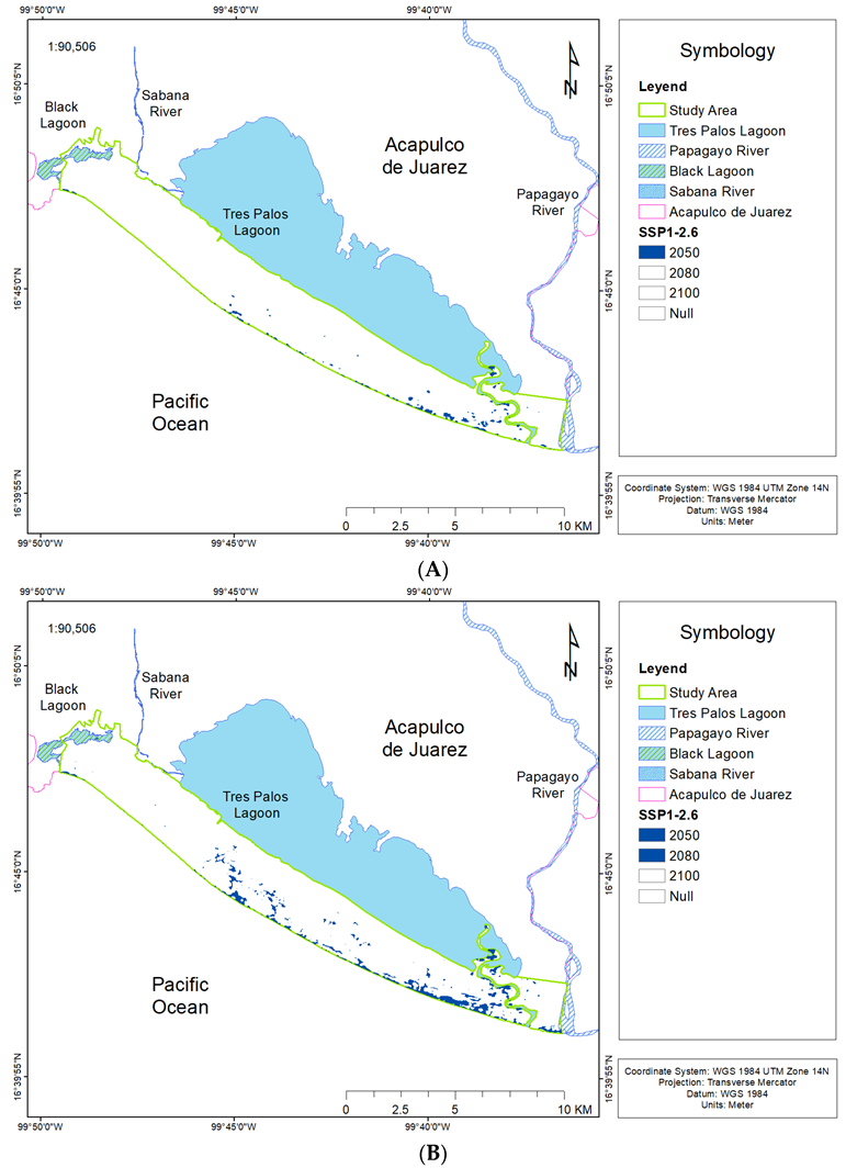
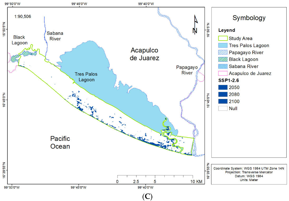
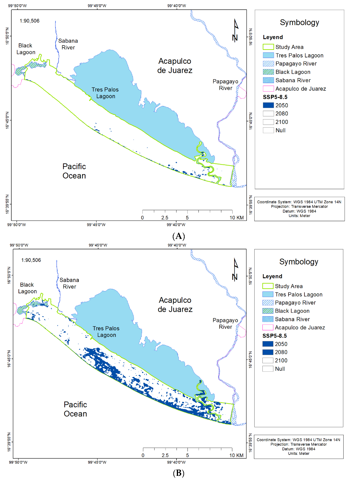
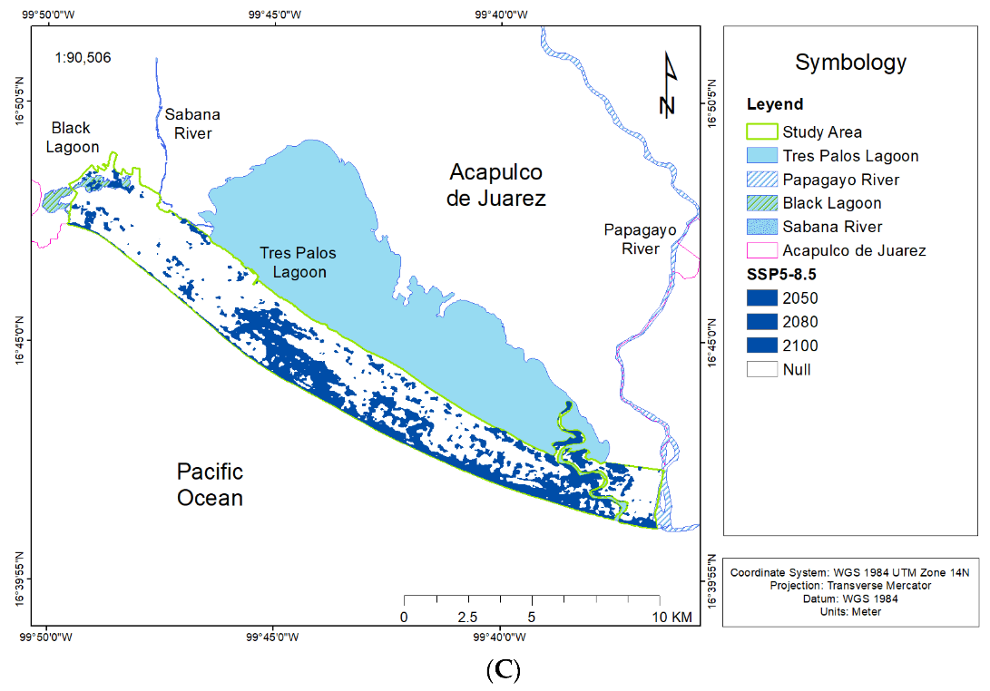
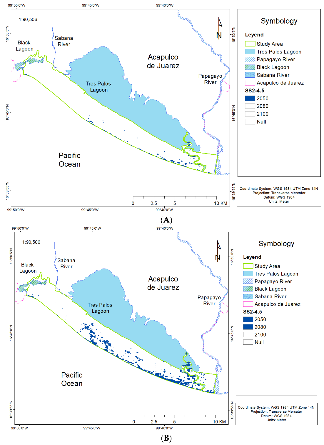
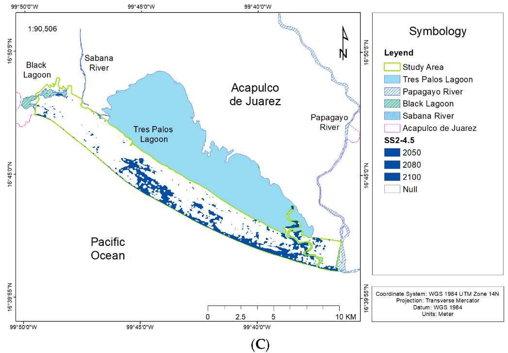
Figure 8C,
Figure 9C, and
Figure 10C show the three prospective scenarios chosen for this study as products of global warming due to climate change: (9c) Optimistic SSP1-RCP2.6, (10c) Conservative SSP2-RCP4.5, and (11c) Extremist SSP5-RCP8.5. Each image shows the maximum flood level for each scenario chosen for 2081–2100.
The areas designated as Null are those that will not be affected by flooding caused by the increase in sea level as a result of climate change until the period 2081–2100. The possibility that these areas may be flooded in subsequent time periods is beyond the scope of this study and will require further analysis of the data.
Along most coasts, local sea level changes can differ by 20% or more from the global mean change, coupled with the effects of long-period tides, and this can significantly increase the frequency of a given extreme water level [
68]. To calculate the percentage and area of flooding, each of the scenarios shown in
Figure 8 used a manual solution. This consisted of creating a database showing the pixel counts of classes containing each of the break values in which the digital elevation model was classified; for the present study, these are 2041–2060, 2061–2080, and 2081–2100 (see
Table 4). As already mentioned, in our digital elevation model, each pixel represents an area of 50 m × 50 m above the ground [
59].
Acapulco Diamante’s total flood zone is likely to increase by approximately 22 km
2 between 2041 and 2060, based on the current coastline, from the boundary of the official Federal Maritime Land Zone for the municipality of Acapulco [
54]—a rise of 0.54 m—and by approximately 540 km
2 for the period 2081–2100 due to a local sea level rise of 2.67 m, compared to the average values for 1995–2014 (
Table 4). A local sea level rise would have repercussions such as frequent road closures, reduced stormwater drainage capacity, deteriorating infrastructure, and saltwater intrusion into drinking water extraction wells. In turn, this would have socioeconomic consequences that would impact restaurant businesses by the sea, tourism service companies, fishing, and many other areas. This point forces us to consider future political plans to mitigate these urban effects.
The results show that the percentage of urban area affected by possible flooding in the SSP1-RCP2.6 scenario would increase from 2% in 2041–2060 to 8% in 2081–2100 (see
Table 5 and
Figure 8), and the percentage of urban area affected by the SSP5-8.5 scenario would increase from 2% to 32% in the same period (see
Table 6 and
Figure 9).
The percentage of the agricultural area that will be affected by 2081–2100 will be approximately 20%, compared to the 1% forecast for 2041–2060, under the SSP2–4.5 scenario, which can be attributed to the greater flood area in 2081–2100 compared to 2041–2060; see
Table 7 and
Figure 10. Agricultural zone flood rates in future scenarios increase significantly the closer we get to 2081–2100; under the SSP5-8.5 scenario, the percentage of flooding in the period 2041–2060 is only 1%, but for 2081–2100, it is an alarming 34%; see
Table 6 and
Figure 9.
4. Discussion
Globally, decision makers and resource managers will be challenged to preserve existing urban and natural habitats. As the first major tourist city on the Mexican Pacific, Acapulco is a representative coastal city. Impacts associated with sea level rise worsen flooding of coastal communities during severe hydrometeorological events and promote erosion, loss of coastal dunes, and loss of habitats.
Through the use of the coastal flood maps generated through the IPESLI method during this study, policy makers can begin to prioritize appropriate responses to future inundation from sea level rise. By providing local elevation values and formulating a time frame in which the greatest impacts of sea level rise inundation may manifest themselves, policy makers can begin to formulate long-term adaptation strategies beyond the current 15-year planning horizon.
The IPESLI procedure proposed here estimated with a high degree of accuracy (above 85%) the prospective effects of sea level rise in a coastal area, since the flood zone showed 87% consistency with water level data. Our method is versatile since satellite images make the remote study possible under non-stationary conditions, particularly in situations such as the pandemic, which has been unfolding since 2019. This allows minimizing field visits in situ. At the same time, it is a comparatively fast, and therefore low-cost, method. A corporation or an academic institution can acquire satellite images that are not freely accessible and can thus substantially improve the data quality.
However, as demonstrated, it is not always necessary for databases to be adjusted with a high degree of accuracy. This could allow this method to be used in other areas where local data on the effect of climate change on the coastal zone are lacking. This will allow for the better calibration and validation of existing models that deal with coastal flooding phenomena, whether they are the product of climate change or are only temporary.
This study has used scenarios supported by sea level rise projections constructed by Kopp et al. (2017) [
31]. These scenarios bear relevance for political decision making at the local level, since they foresee the need for adaptation by estimating, in advance, the retreat of coasts on mainlands and islands of low altitude, which will be very vulnerable during the second half of the 21st century. Creating a shared framework of vital information on sea level rise is essential for better supporting stakeholders, and especially coastal decision makers.
Incorporating climate change science, and specifically the science around sea level rise, into the updating of existing laws and the creation of new public policy is challenging [
69]. Providing information with spatial data and imagery can help reduce personal discretion in decision making by public administrators [
70]. In the context of coastal planning, it has been suggested that a top-down approach with the presence of strong leadership is the best way to eliminate discretion [
71].
A few international research projects have focused on risk management and adaptation, specifically designed for small-scale coastal zones, where satellite images have been used to generate maps showing expected sea level rise levels. An increase of about 25% in inundation area is expected by 2100 in the central region of Singapore [
72]. By 2070–2080, the Bengal tiger is expected to have lost the entirety of its natural habitat in the Sundarbans mangrove forest in southwestern Bangladesh [
73]. Depending on the RCP-SSP projection, an inundation area in San Francisco Bay of between 90 and 218 km
2 is expected [
74]. Entire coastal dune habitats worldwide are expected to be reduced as a result of permanent sea level rise [
75]. The Guadeloupe area is expected to present future chronic flooding and severe impacts given the high urbanization [
76].The results of our study represent a step in the right direction with respect to the lack of spatial information for sea level rise projections for the Mexican South Pacific coast. These types of studies increase the awareness of the community that will have to deal with permanent increases in the coastal strip, which will lead them to implement new adaptation strategies to cope with potential future economic, natural, and cultural impacts. Therefore, this analysis provides a new tool for public administrators to monitor and evaluate at-risk areas in order to prevent the loss of property and potentially future human lives.
The simulated flood magnitudes related to local sea level rise may be overestimated because future structural flood control measures have not been considered (since there are none) and also because of the micro details of the topography in the model’s configuration. In addition, the above results should be considered in the context of implicit error. Factors such as buildings, vegetation, terrain slope, and random noise can cause vertical errors in elevation data, leading to the incorrect classification of areas as safe or risky. Different elevation data sources also contain errors, both in their typical range and in their average.
In subsequent studies, an analysis of morphological conditions (estuary areas, retro-dune areas, old emissaries of the lagoon filled up, etc.) is recommended. For example, in the case of the Acapulco Diamante coast, the role of the lagoon’s emissary cannot be denied.
5. Conclusions
This article concludes that, if the increase in global temperature stops at 2 °C in relation to 1850–1900, it is possible that, by 2081–2100, up to 5% of the study area will be affected by extreme floods, leading to approximately 78 km2 of flooded land. If we reach 3 °C, 24% of the zone could be flooded (approximately 371 km2), and it could be 35% if we reach 5.7 °C, representing up to 541 km2 of flooded land. Future research may exclude several scenarios that cannot be ruled out today. However, the effects of local subsidence may continue to contribute to future relative sea level changes in some areas, and these need to be characterized. To determine the regional consequences of global phenomena such as global warming, the constant and systematic monitoring of phenomena such as sea level increases is required.
The IPESLI procedure presents a proof-of-concept for a policy-making tool designed to graphically show the impact that sea level rise could have on a low-elevation coastal area. The methodology allows high quality estimates to be achieved, while, at the same time, it is applicable to all coastal areas of the planet, taking into account that its cost-benefit is relatively low in relation to the available data and resources. The coastal inundation maps created in this study can be used to identify the most vulnerable areas and initiate decision making that will benefit both wetland and coastal areas, as well as nearby communities, and should be taken into account for conscious land-use planning and the creation of climate adaptation strategies.
Although the exercise is still perfectible, and improvements can always be made, the present procedure has the potential to contribute to forming a communication bridge between climate change science and local decision makers, which will contribute to moving sea level rise adaptation in the right direction. Implementing this type of methodology through citizen science initiatives such as observatories could account for the constant evolution of projections for this problem. In the same way, it would make visible a problem that has been little discussed in the local and national public spheres due to our perceived remoteness from the consequences of these phenomena.


 ,
, 


