1. Introduction
Economic and financial time series may exhibit many distinctive characteristics, including the presence of serial correlation, stochastic or deterministic trends, seasonality, time varying volatility, and nonlinearities. However, when the focus of the analysis is on the relationships among various variables, it is commonly observed that one or more of these features detected in individual series are common to several variables. We talk about common features when such features are annihilated by some suitable linear combinations of variables (
Engle and Kozicki 1993). The most well-known example is probably cointegration, which is the presence of common stochastic trends (
Engle and Granger 1987). Other forms of comovements have also been studied, giving rise to developments around the notions of common cyclical features (
Vahid and Engle 1993), common deterministic seasonality (
Engle and Hylleberg 1996), common volatility (
Engle and Susmel 1993), cobreaking (
Hendry and Massmann 2007), etc. Recognizing these common feature structures presents numerous advantages from an economic perspective (e.g., the whole literature on the existence of long-run relationships), but there are also several benefits for statistical modeling. Indeed, imposing the commonalities in estimation reduces the number of parameters, thus potentially leading to efficiency gains in statistical inference and improvements in forecasts accuracy (
Issler and Vahid 2001). Moreover, the presence of common dynamics can be used for analyzing and forecasting large dimensional systems (
Cubadda and Hecq 2011,
2022a;
Bernardini and Cubadda 2015).
Building on the common feature approach, we propose the detection of common bubbles in stationary time series. Intuitively, the idea is to detect bubble patterns in univariate time series and then to investigate whether those bubbles are common to a set of assets. In the affirmative case, a portfolio composed of those series would not have such a nonlinear local explosive characteristic. There are several ways to capture bubbles in the data. We rely on mixed causal–noncausal models (denoted as MAR
hereafter), namely autoregressive time series that depend on both
r lags and
s leads. Indeed, there has been recent interest in the properties of noncausal processes associated with a blooming of applications on commodity prices, inflation or cryptocurrency series, and the developments around the notion of nonfundamental shocks, see, i.a.,
Hecq and Voisin (
2022) and the references therein. We choose to consider mixed causal and noncausal, models as they might also be used for forecasting. This is not necessarily the case with other approaches aimed at identifying bubble phases.
A first attempt into this direction was made by
Cubadda et al. (
2019), who extended the canonical correlation framework of
Vahid and Engle (
1993) from purely causal vector autoregressive models (namely the traditional serial correlation common feature approach within a VAR) to purely noncausal VARs (a VAR with leads only). They showed that different forms of commonalities can emerge when we also look at VARs in reverse time. However, their approach, being based on either canonical correlation analysis or the general method of moments, do not work for mixed models where non-Gaussianity of the error terms is required for identification, see e.g.,
Lanne and Saikkonen (
2013).
In this paper, we extend their work and we propose a Student t-distribution maximum likelihood (ML henceforth) framework to compare the multivariate mixed causal–noncausal model with
r lags and s leads (VMAR
hereafter) with a restricted version where a reduced rank structure is imposed on the lead polynomial matrix. This is our notion of common bubbles, which is equivalent to requiring that there exist linear combinations of variables exhibiting bubbles that no longer possess the bubble feature. See for instance
Cubadda and Hecq (
2022b) for a recent survey on reduced rank techniques for common feature analysis. We consider both likelihood ratio tests and information criteria for our purposes.
Given that explosive roots and noncausal dynamics in VARs are intimately related (see, e.g.,
Gourieroux and Jasiak (
2017) and the references therein), our approach has a similar spirit as the one of
Engsted and Nielsen (
2012), who proposed a test for the hypothesis that stock prices and dividends possess a common explosive root. Possible comparative merits of our methodology are that it does not require the prior knowledge of the value of the common explosive root and that as we work with stationary VMAR models, only standard asymptotic theory applies.
The rest of this paper is organized as follows: in
Section 2 we establish the notations for multivariate mixed causal and noncausal models. Contrary to the univariate case, two distinct multivariate multiplicative representations lead to the same additive form of the VMAR
. Consequently, such alternative representations have the same likelihood but with different lag–lead polynomial matrices. We advocate the use of the multiplicative representation where the lead polynomial matrix is the first factor since the alternative representation does not allow for the easy unraveling of the presence of common bubbles. Within a Student t-distribution ML framework, we explain how to implement both likelihood ratio tests and information criteria to detect the existence of common bubbles.
Section 3 investigates, using Monte Carlo simulations, the small sample properties of our strategy for bivariate and trivariate systems both under the null of common bubbles and the alternative of no rank reductions.
Section 4 illustrates the practical value of our approach with an empirical analysis of three commodity prices.
Section 5 concludes.
2. Multivariate Mixed Causal–Noncausal Models
Recall that a univariate MAR(
) model is constructed as follows:
where
is the lag operator such that
and
is the lead operator such that
. Since all the coefficients are scalars, the polynomial product is commutative and the representation
will yield the same model parameters as the previous one. The error term
is assumed to be i.i.d. and non-Gaussian for identification purposes.
Let us now consider the case where
is an
N-dimensional stationary process. For the sake of simplicity, we assume that deterministic elements are absent. Analogously to the univariate case, the VMAR
, is defined in its multiplicative forms as follows:
where
Both models (
1) and (
2) are equivalent in the sense that they generate the same time series, but due to the noncommutativity property of the matrix product, they are two distinct representations of the same process. Specifically, the lag polynomial matrices
and
, although of the same order
r, have unequal values of the coefficient matrices, and the same observation applies to the
order lead polynomial matrices
and
as well.
We assume that
and
are i.i.d. and follow multivariate Student t-distribution with location zero. We could consider different distributions as long as they are non-Gaussian. This is indeed the condition that allows for distinguishing the genuine VMAR
specification from the so-called pseudo causal and noncausal representations, see
Lanne and Saikkonen (
2013) for details.
We further assume that the roots of the determinant of each of the polynomial matrices , are outside the unit circle to fulfill the stationarity condition. Furthermore, we will show later that the distribution of the errors and have identical degrees of freedom but different positive definite scale matrices, which are respectively denoted by and .
Let us respectively denote with
and
the products of the lag and lead matrix polynomials of the two models (
1) and (
2):
1
The general forms of the product of the lead and lag matrix polynomials for both the representation respectively read as follows:
with
and
. Hence, both the multiplicative representations yield exactly the same additive form
where
follows a multivariate Student t-distribution with degrees of freedom
, as
and
in representations (
1) and (
2), and with a scale matrix
. The lag polynomial in (
3) is the following:
An example of derivation of the polynomial matrix
for VMAR
is given in
Section 2.1.
In summary, contrary to the univariate case, a VMAR
process has two distinct multiplicative representations. ML inference can indifferently be performed with each of the two representations (
1) and (
2). However, both representations will correspond to the same additive form of the model in Equation (
3). This makes the interpretation of the lag and lead coefficient matrices in the multiplicative forms more intricate.
Lanne and Saikkonen (
2013) advocated for the use of one or the other representation depending on the analysis performed; one representation might be easier to employ for certain inquiries.
2.1. Common Bubbles in VMAR(r,s)
Having discussed the main properties of the unrestricted VMAR, we consider additional restrictions coming from a reduced rank structure in the lead polynomial matrix in order to model
common bubbles. Notably, the noncausal component explains the growth phase of the bubble, whereas the causal component determines the burst phase (
Gouriéroux and Zakoïan 2017). Hence, it is the multiplicative structure of the VMAR, combined with heavy tailed errors, that captures the nonlinearity of the bubbles as a whole. However, without the noncausal component, heavy tailed errors in a causal AR setting would not be able to reproduce locally explosive episodes. Although the focus in this paper is on common bubbles, our approach can be easily extended to investigate commonalities in the causal part or in both the lag and the lead components.
Definition 1. An N-dimensional VMAR process displays common bubbles (CBs hereafter) if there exists a full-rank matrix δ of dimension , with , such that, for , where the coefficient matrix is defined in (4). This implies that the coefficient matrices can be factorized as where is the orthogonal complement of such that and constitute a matrix with dimensions . For the sake of simplicity, let us start the analysis from the case
. The coefficient matrices of the leads in the additive representation (
3) with reduced rank restrictions are as follows:
where the matrices
and
are as follows:
When
k CBs exist, the matrix
annihilates the forward looking dynamics
This implies for the second lead coefficient matrices that
Since
(resp.
) cannot be equal to zero, it follows that
(resp.
), with
(resp.
) being a full-rank
dimensional matrix, and thus
(resp.
). Hence, both
and
must have rank
but potentially different left null spaces (see also
Cubadda et al. 2019).
By premultiplying the first lead coefficient matrix of representation (
1) by
, we have
which implies that
and
must have the same left null space. Moreover, keeping in mind that
, we have
which shows that
and
have the same left null space as
and
, respectively.
By premultiplying the first lead coefficient matrix of the alternative representation (
2) by
, we instead have
which implies that the matrix
might not even have a reduced rank.
It is easy, although tedious, to see that the same conclusion holds for any VMAR. We summarize these results in the following proposition.
Proposition 1. In the presence of k CBs in an N-dimensional VMAR process, we have in (1), whereas in (2). Hence, the same linear combinations annihilate the lead coefficient matrix both in the additive representation (3) and in the multiplicative representation (1) but not in the alternative multiplicative representation (2). This implies that the coefficient matrices can be factorized as for . 2.2. Testing for Common Bubbles
In view of Proposition 1, a likelihood ratio test (LRT henceforth) for the presence of
k CBs requires the comparison of the likelihood value of the unrestricted model (
1) with the likelihood value of the restricted model:
Since
has dimension
with
, there are
possible reduced-rank models to consider for all possible
k. Furthermore, since the matrix
can be normalized such that
it has only
free parameters in
.
A sample
Y of
T observations drawn from an
N-dimensional VMAR(
) process with i.i.d.
t-distributed errors has location 0, a positive definite scale matrix
, and degrees of freedom;
has the following log-likelihood function
where
Without any commonality restrictions,
is given either by (
1) or (
2), depending on the representation chosen for the estimation. For the estimation of the likelihood function with commonality restrictions,
is given by (
5), where normalization (
6) is imposed for identification of matrix
.
2 Hence, imposing the restrictions within the Student’s
t-ML estimation framework of the MVAR model is straightforward. The LRT is then constructed as follows
where
and
are, respectively, the likelihood values associated with the restricted model (
5) and with the unrestricted one (
1). Under the null of
k CBs, (
7) follows an asymptotic
distribution with
degrees of freedom.
One can also perform an LRT for the null hypothesis such that the
versus the alternative
k with
. The associated LRT statistic is as follows:
which is asymptotically distributed as a
distribution with
degrees of freedom.
An alternative is to select the best specification according to the minimization of an information criterion as follows:
with
being the number of coefficients estimated in a model with
CBs for
.
3. Monte Carlo Analysis
We investigated the performance of our strategies using Monte Carlo simulations to detect the common bubbles in bivariate and trivariate VMAR(1,1) models. We considered two sample sizes,
and 1000, and two different degrees of freedom of the error term with very leptokurtic distributions, namely
, to respectively consider a finite and infinite variance case. We employed lead coefficient matrices with and without reduced rank to analyze the detection of the correct model under the null of common bubbles and under the alternative of no such comovements. The coefficients employed in the bivariate settings are displayed in
Table 1.
The results, based on 3000 replications for each combination of parameters, are reported in
Table 2.
3 All entries are the frequency of correctly detected model. That is, under the null of a CB, we report the proportion of correctly detected CB, and under the alternative of no CB, we report the proportion of correctly rejected CB. We hence performed the test
against the alternative that the rank is 2. The LRTs were performed at a 95% confidence level. The information criteria detected a CB when the IC of the restricted model was lower than the one of the unrestricted model.
We can notice that the frequency of type I errors of the LRT increases when the variance of the errors becomes infinite and that it does not significantly decrease when the sample size gets larger. With finite variance (), the LRT has an appropriate size of around 5.5%, and it increases to around 8.6% when the degrees of freedom of the error distribution reach 1.5. Under the alternative, the LRT has a power of at least 99.9% across all parameter combinations, implying that it almost never detects a CB when there are none.
Regarding the model selection using information criteria, results show that BIC outperforms AIC. Under the null of a CB, BIC selects the correct model specification in 98.9% of the cases with finite variance and a sample size of 500. The frequency increases to 99.3% when the sample size increases to 1000. AIC, on the other hand, selects the correct model in only 83.8% of the cases and does not increase with the sample size. The frequency of the correctly selected model decreases for both when in the infinite variance case, but more drastically for AIC, which decreases to around 78%. BIC still selects the correct model for 96.8% of the cases with a sample size , and the frequency increases to 97.7% for . Under the alternative of no CB, however, both ICs correctly select the unrestricted specification in more than 99.4% of cases across all parameter combinations.
We now turn to the trivariate case. In the presence of a CB, the rank of the lead coefficient matrix can be either 1 or 2. We thus consider the two possible CB structures. The parameters of the data generating processes are displayed in
Table 3.
We evaluated our approach with 1500 replications with each of the parameter combinations. Under the null of a CB, we tested the correct CB specification against the alternative of the unrestricted full rank model. Under the alternative of no CB, we tested for each of the CB specifications.
4 Table 4 reports the frequencies of the correctly detected models either with the LRT or with model selection using the information criteria. Analogously to the bivariate case, the LRTs were performed at a 95% confidence level, and the information criteria detect a CB when the IC of the restricted model was lower than the one of the unrestricted model.
We can notice that the size of the LRT when the true rank of the lead coefficient matrix is 2 is similar to the bivariate case. With a finite variance error distribution, the size of the LRT is around 5%, and it increases to around 9% when the variance is infinite (
). We can see that the size of the test decreases in the more restrictive CB specification when the rank of the matrix is 1. For the finite variance cases, the size decreases to 91.9% when
and to 93.3% when
. The correctly detected model frequency decreases further to 86% in the infinite variance case. Under the alternative of no CB, with finite variance and a sample size of
, the LRT incorrectly detects a bubble (
2 vs. 3) in 30.5% of the cases; however, this frequency decreases to 6.8% when the sample size increases to 1000. Hence, it seems that with a smaller sample size and the finite variance of the error distribution, estimating 8 coefficients in the lead matrix instead of 9 in the unrestricted model still provide a good enough fit to not be rejected by the test. The power of the test for all other model specification is above 99.7%.
5As it relates to the model selection using information criteria, BIC outperformed AIC in detecting common bubbles in each of the settings. BIC correctly selected a model with CBs in more than 97.2% of the cases across all model specifications, and the frequencies increased with the sample size and the amount of restricted coefficients. Indeed, it correctly selected a restricted model with a coefficient matrix of rank 1 in at least 99.8% of the cases, whereas AIC selected the correct restricted model in fewer than 88.3%. The frequency decreased with the sample size as did the variance of the errors when the rank of the restricted matrix was closer to full rank. Hence, for the infinite variance case with a sample size , its frequency of correctly selected CB model is around 77.5% for each of the CB specifications. Under the alternative of no CB, we observe the same pattern as that for the LRT. In the finite variance case, both information criteria overselected a restricted model with a matrix of rank 2. For a sample size of 500, BIC selected the restricted model in 51.9% of the cases although it decreased to 19.8% when the sample size increased to 1000. AIC, on the other hand, only selected the restricted model in 14.5% with and it even decreased to 3% with . For all other model specifications, both IC selected the correct model in at least 99.4% of the cases.
Overall, the size of the LRT seems to converge to 5% in the finite variance cases when the sample size increases. In the infinite variance cases, the size is around 5 percentage points lower and seems to be less affected by the sample size. The power of the test is above 93% in all model specifications except with
and
, with a restricted model that has only 1 coefficient less to estimate than the unrestricted model (
2 vs. 3). For the model selection using information criteria, BIC overall outperforms AIC in correctly detecting a CB but also tends to detect a CB more often than does AIC when there is none in the
2 vs. 3 case with
.
6 4. Common Bubbles in Commodity Indices?
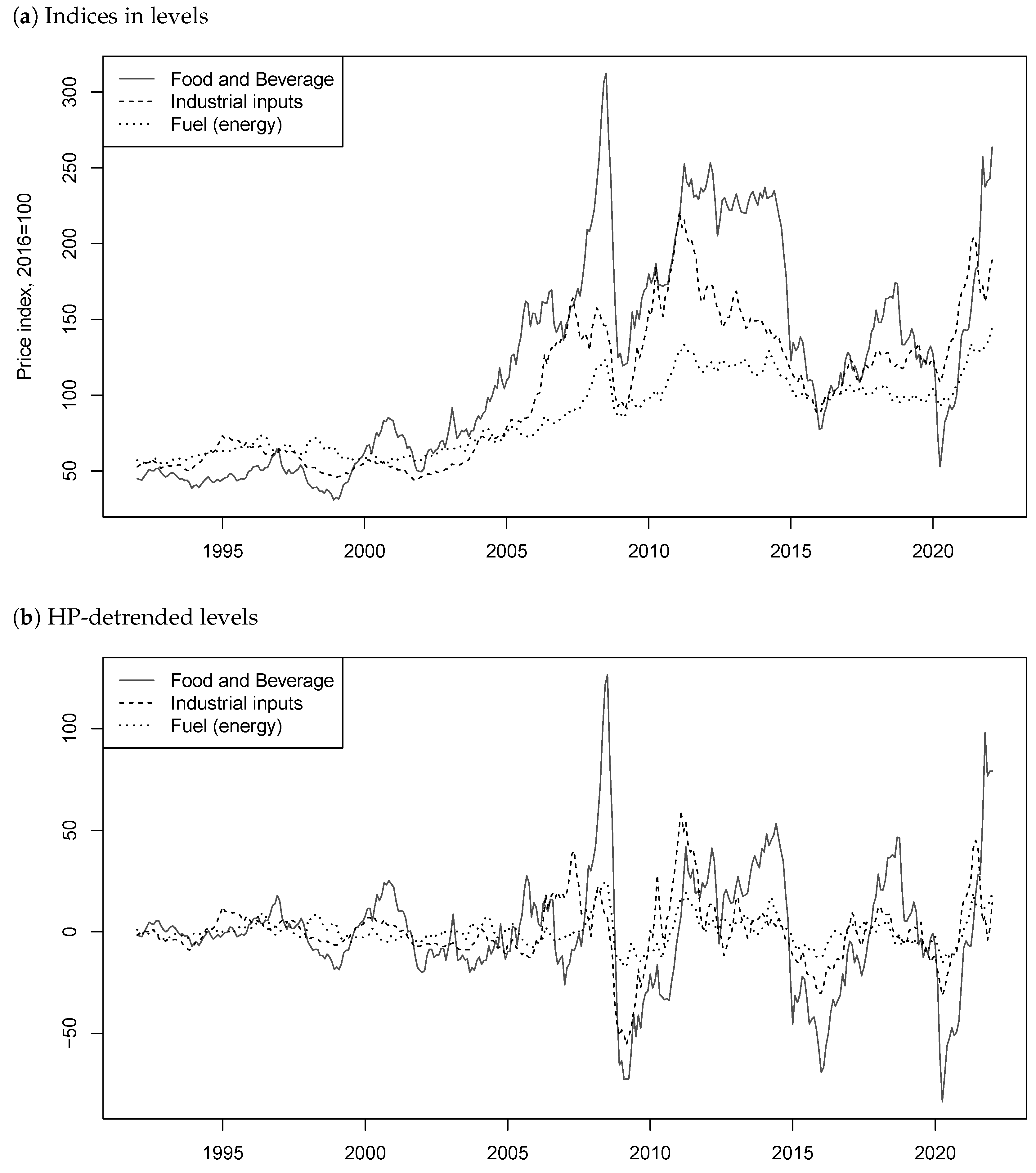
We illustrate our strategies in testing for common bubbles in mixed causal–noncausal processes on three commodity price indices: food and beverage, industrial inputs
7 and fuel (energy)
8. The sample of 362 data points ranges from January 1992 to January 2022.
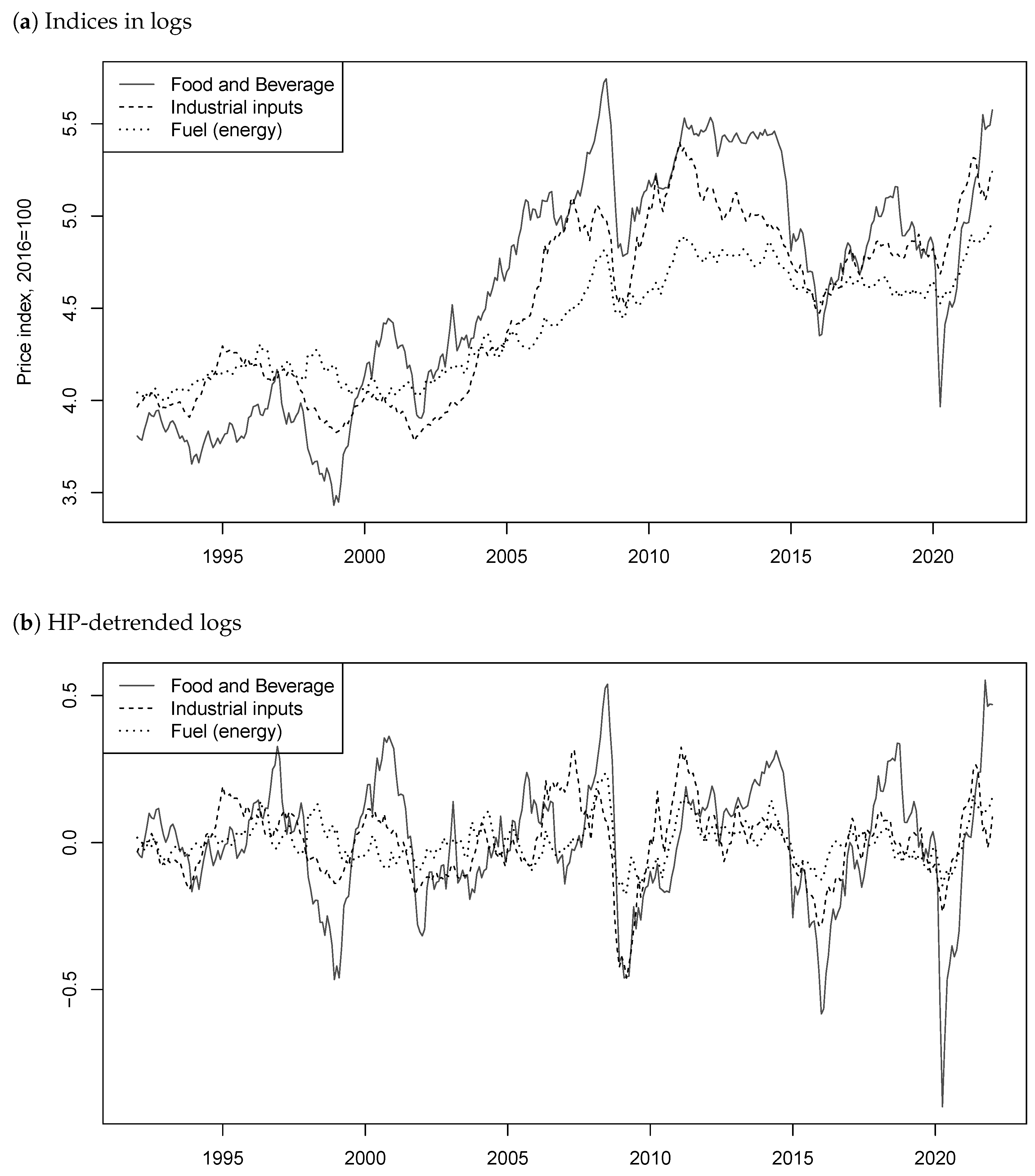
9 We can see from graphs (a) of
Figure 1 and
Figure 2, which respectively show the series in levels and logs, that the indices seem to follow similar trends. Long-lasting increases and crashes roughly occur at the same time. This could potentially suggest the presence of common bubbles between the series.
Following the work of
Hecq and Voisin (
2022), we detrend all series using the Hodrick–Prescott filter (hereafter HP filter). Although this approach to obtain stationary time series has been strongly criticized, in particular for the investigation of business cycles,
Hecq and Voisin (
2022) show that it is a convenient strategy to preserve the bubble features. They also show in a Monte Carlo simulation that this is the filter that preserves the best identification of the MAR(
) model.
Giancaterini et al. (
2022) arrive at the same conclusion using analytical arguments.
The HP detrended series are displayed on graphs (b) of the two Figures. It can indeed be seen that the dynamics inherent to mixed causal–noncausal processes mentioned above are preserved. The that occurred during the financial crisis of 2007 and the COVID-19 pandemic in 2020, while being of different magnitudes, happened roughly at the same time on all three series. Furthermore, long lasting increases such as the one before the financial crash and the recovery around 2009 or after 2020 are also present in all three index prices.
We first analyzed the series individually. We estimated pseudo causal autoregressive models to identify the order of autocorrelation in each of the detrended series (both in levels and logs). All the models that we identified using BIC were ultimately AR(2) processes. The normality of the errors was rejected for all series: values of the Jarque–Bera statistics ranged between 48 and 253 for the 6 series. The next step was to identify MAR() models for all r and s subject to the constraint , namely MAR(), MAR() or MAR(). Based on the ML estimator with Student’s t-distributed error term, the best fitting model for all six series was the MAR() model.
The estimated models are shown in
Table 5.
10 For comparison purposes with the trivariate case shown later, we display both the coefficients estimated from the multiplicative
and the associated coefficients of the linear form obtained as follows:
It appears that “food and beverage” and “industrial inputs” are both mostly forward looking with lead coefficients close to 0.85 and lag coefficients around 0.4. Conversely, the “fuel index” appears more backward looking with coefficients inverted. Except for the level of industrial inputs, all models have error terms with finite variance, and as expected, one obtains lower variance for the logs of the series. The similar dynamics between food and beverages and industrial inputs could indicate commonalities. The same conclusions can be drawn from the coefficients of the linear form.
For the multivariate investigations, we analyzed both bivariate and trivariate systems. Similarly to the univariate estimation, the strategy consisted of first estimating the pseudo lag order
p using a standard VAR(
p) for the six bivariate combinations (three in levels and three in logs) and the two trivariate models. Using BIC, all VARs were identified as VAR(2). There were starting value issues when estimating VMARs by ML, meaning that we often reached local maxima. To avoid this issue, we used a large range of starting values to estimate VMAR(1,1) with multivariate Student’s
t-distributed errors, and we kept the estimated model with the highest likelihood value.
11The estimated models are shown below in
Table 6. We used representation (
1) for the estimation, but the coefficients displayed are those of the additive form (
3), which are independent of the representation used for the estimations in the following form:
where
follows a multivariate Student’s
t-distribution with
degrees of freedom and correlation matrix
.
In comparison to the coefficients
and
of the univariate linear forms in
Table 5, the directions and magnitudes of the dynamics have been preserved in the multivariate model estimations. From the off-diagonal coefficients of the bivariate models, we can notice that “Food” is impacting both “Indus” and “Fuel” with the lag and the lead, with coefficient magnitudes between 0.11 and 0.47 for the levels. However, in the other direction, the magnitude of the coefficients does not exceed 0.05 for the lag of “Fuel” on “Food”. “Fuel” slightly impacts “Indus” with coefficients of magnitude around 0.1. These dynamics can also be observed in the trivariate model.
To perform the common bubble tests, we estimated VMAR models with restrictions on the lead coefficients matrix as shown in (
5).
12 In the trivariate settings, the LRTs and information criteria compare the unrestricted model where the lead matrix has full rank with both CB specifications, namely imposing rank 2 or rank 1 to the lead coefficient matrix.
The results are shown in
Table 7. The LRT column displays the LRT statistic, and the IC columns are the difference in the IC values of the restricted and the unrestricted models. As can be seen from the LRTs, the null hypothesis of a common bubble in the bivariate and trivariate models is rejected for all combinations of variables at a confidence level of 95%. All information criteria also indicate a better fit for the models without commonalities since all values are positive. Even for the trivariate cases
2 vs. 3, no bubble can be detected even though in the simulations exercise, the test and information criteria overdetected a CB for the same sample size and degrees of freedom. Hence, while the series seem to follow a similar pattern in the locally explosive episodes throughout the time period, we did not find there to be a significant indication of commonalities in their forward looking components.
There are two possible explanations for these findings. First, our definition requires that bubbles occur at the same time for all the series, whereas graphical evidence may suggest the presence of some degree of nonsynchronicity in the bubble patterns among variables. Second, the series apparently display uncommon explosion rates of the locally explosive episodes.


