
Maximum Likelihood Inference for Asymmetric Stochastic Volatility Models

1
Canvas Capital S.A., Sao Paulo 04538-000, Brazil
2
Department of Statistics, University of Campinas, Campinas 13083-859, Brazil
*
Author to whom correspondence should be addressed.
Econometrics 2023, 11(1), 1; https://doi.org/10.3390/econometrics11010001
Submission received: 3 September 2022
/
Revised: 19 December 2022
/
Accepted: 20 December 2022
/
Published: 23 December 2022
Abstract
:In this paper, we propose a new method for estimating and forecasting asymmetric stochastic volatility models. The proposal is based on dynamic linear models with Markov switching written as state space models. Then, the likelihood is calculated through Kalman filter outputs and the estimates are obtained by the maximum likelihood method. Monte Carlo experiments are performed to assess the quality of estimation. In addition, a backtesting exercise with the real-life time series illustrates that the proposed method is a quick and accurate alternative for forecasting value-at-risk.
1. Introduction
Since the seminal paper of Black (1976), one of the most studied empirical regularities in the financial econometrics literature is the inverse (asymmetric) relationship between return and volatility. For instance, in equities, a higher increase in volatility is observed after a negative return compared with a positive return. This stylized fact is called the leverage effect. For a discussion of this topic, see McAleer (2014).
Stochastic volatility (SV) models, first proposed by Taylor (1982), are characterized by the presence of two random disturbances: one in the return equation and the second in the log-variance equation. In this family of models, the asymmetry of volatility can be included via the correlation of the two disturbances; see Taylor (1994) and Harvey and Shephard (1996)1.
Since then, several works have presented methods for estimating asymmetric stochastic volatility (A-SV) models. We can cite Jacquier et al. (2004); Selçuk (2005); Omori et al. (2007); Jensen and Maheu (2010); Asai and McAleer (2011); Nakajima and Omori (2012); Jensen and Maheu (2014) and Hosszejni and Kastner (2021). These are Bayesian proposals and in most of them, the estimation is carried out by MCMC procedures.
The main objective of this paper is to propose a new method for estimating A-SV models. Our proposal combines the framework of Shumway and Stoffer (2006, chp. 6) for SV models and the approximation method proposed by Omori et al. (2007). The estimation is carried out by maximum likelihood and does not involve simulations, such as in MCMC or importance sampling methods. We also present a procedure for forecasting the value-at-risk, a topic that is not discussed in most works related to A-SV models.
The proposed method has several advantages. First, it works for multiple A-SV specifications, where the perturbations in the return equation can be non-Gaussian. Second, the estimation procedure is very quick (it takes only a few seconds), which is a very important feature for practitioners. Third, out-of-sample value-at-risk forecasts can be quickly and easily obtained.
The results obtained in Monte Carlo experiments evidence that the proposed method is good in terms of point estimations. Additionally, the proposal performs well when estimating value-at-risk forecasts in the stock market and exchange rates in the return time series.
The results of our proposal, both in the simulated data and real-life dataset, are compared with those obtained using the Bayesian method implemented in the stochvol package of R (R Core Team 2020). Among the Bayesian alternatives, this method was chosen because it is easily available and is very quick.
There are alternative methods for modeling the asymmetry of volatility in SV models. For example, asymmetric behaviors are included explicitly in the log-variance equation in Mao et al. (2020), while Schäfers and Teng (2022) discuss some specifications where the parameters of the log-variance dynamics change after a positive/negative return. Finally, Takahashi et al. (2021) modeled the asymmetric behavior in the realized volatility using a realized SV model. We do not discuss these approaches here.
The paper is organized in five sections, including this Introduction section. The proposal is presented in Section 2. To assess the performance of the proposed method, Monte Carlo experimental results are described in Section 3. Empirical illustrations are presented in Section 4. Section 5 contains the principal conclusions, and the derivation of the Kalman filter is described in the Appendix A.
2. Methods
Here, the proposed method and its implementation are described in the first three subsections. Then, brief comments about a comparison method are presented.
2.1. Parameter Estimation
Let be a sequence of returns. The asymmetric stochastic volatility (A-SV) model is given by the following:
where is a sequence of independent identically distributed bivariate random variables with a mean vector of and the following covariance matrix.
Normally, it is assumed that () follows a bivariate normal distribution (see, for example, Omori et al. (2007)). In our proposal, as in Jensen and Maheu (2010) and other approaches in the literature, we relax the bivariate normality assumption but maintain .
In the AS-V model the impact of returns on the volatility depends on the correlation between and , . Thus, if and the other parameters remain constant, positive returns produce an increase of the expected log-volatility; see Yu (2005). Likewise, if , then negative returns produce an increase in log-volatility. Therefore, the parameter controls for the leverage effect.
From Equation (1), taking the logarithm of the squares, we have the following:
where , , and . Since is not normally distributed, the system formed by Equations (4) and (2) constitutes a non-Gaussian state-space model. In consequence, we have to tackle two problems: non-normality and the dependence structure in .
In the case of , Shumway and Stoffer (2006, chp. 6) provide a maximum likelihood estimation method. The idea of this method is to approximate the distribution for by using a mixture of normals:
where with , and is a sequence of independent Bernoulli variables with . Therefore, adopting the framework of dynamic linear models with Markov switching, the states are associated with the m terms of the mixture, and the expressions of the Kalman filter are readily obtained because we have a Gaussian conditional distribution given a state.
Next, we describe a modification of the above method to account for the correlation between and , i.e., when .
Second, we approximate the conditional distribution of by following an approach similar to that presented by Omori et al. (2007). For instance, let , where is the indicator function that is equal to one if the argument is true and zero otherwise. Therefore, it is possible to map to as follows:
and then and .
Our objective is to approximate by a mixture of normals assuming that satisfies Equation (5). As a consequence, we have an additional problem to tackle because we need to evaluate quantity . Thus, we follow the approach presented in Omori et al. (2007), where is approximated by the following:
and quantities and , for , are obtained by minimizing the mean square norm.
By solving this problem, we obtain and . Then, the approximation of is given by the following.
Third, from the previous result and using the approach of Omori et al. (2007), the joint distribution of that is conditional on and satisfies the following:
with . Therefore, from Equation (11), we obtain the following:
where is calculated as for .
Using Quantities (12) and (13), we can derive the Kalman filter algorithm’s expressions in a similar way as performed in Shumway and Stoffer (2006, chp. 6); see the Appendix A for details. These expressions are as follows:
for where the probabilities are calculated by the following equation:
with density being approximated by :
and given values for
Then, the log-likelihood is evaluated by the following equation:
with for , and the maximum likelihood estimates are obtained by optimizing (21) using numerical routines.
There are three differences in our approach compared with the work of Omori et al. (2007). First, as described earlier, we are not restricted to the case when the distribution of is a bivariate Gaussian distribution. Second, we estimate the parameters by maximum likelihood while Omori et al. (2007) used an MCMC algorithm. Third, their work considered an approximation of a mixture of 10 terms with known values for and , and it is only valid when . In contrast, in our approach, quantities and for are estimated by usually involving a smaller number of mixtures, such as .
2.2. VaR Forecasting
We follow the same strategy presented by Abbara and Zevallos (2019, 2022) for VaR forecasting. Thus, given the sample of returns , we perform the following:
- 1.
- Estimate the parameters for .
- 2.
- From the Kalman filter, calculate for and obtain the predicted volatilities , where .
- 3.
- Obtain the standardized residuals for and compute the -quantile of , which is called .
- 4.
- The %-VaR is then equal to
Note that since our model is semiparametric in the sense that only the first two moments of the distribution of are specified, and we use the standardized residuals to estimate the distribution of . This adds flexibility compared to parametric approaches in the literature.
2.3. Implementation
All codes were written using the R language (R Core Team 2020). The Kalman filter algorithm is implemented using the Rcpp and RcppArmadillo packages, and we use the nlminb function to perform the numerical optimization needed to obtain parameter estimates.
The initial values of the parameters are , , , , (except for ), and for . Additionally, for the Kalman filter, we use as initial values and probabilities for .
2.4. The Stochvol Method
We compare our method with the algorithm available in the stochvol package of R where the estimation of A-SV models is performed by Bayesian MCMC methods. Details about the priors for each parameter and other estimation steps are presented in Hosszejni and Kastner (2021).
For each parameter in , the package provides a sample from the posterior distribution when or . We choose the sample’s mean of the posterior sample as the point estimate (which minimizes the quadratic loss function).
The stochvol package also provides the posterior distribution of the volatility, , for . We consider the sample mean of this posterior as the point estimate of the volatility. Furthermore, the -VaR calculated from stochvol is the quantile of the predictive distribution for , which is also provided by the package.
3. Monte Carlo Experiments
The performance of the proposed method is assessed here by performing Monte Carlo experiments. Models (1)–(2) were simulated by considering an around −7.36, , and three pairs of values for and : (, ), (, ), and (, ). These sets of parameters were chosen based on the empirical results presented in Section 4. In addition, we considered two different distributions for , the standard normal distribution and a standardized t-Student distribution with degrees of freedom, denoted by . To simulate the bivariate distribution of for the latter case, we used , where follows a standardized Student’s t-distribution with degrees of freedom, and . Then, as required, we used the following: , , and .
For each combination of parameter values and distribution, we simulated 1000 samples of , and the performance was assessed by the bias, standard deviation (SD), and the root mean square error (RMSE).
The proposed method was implemented using to evaluate the sensitivity to the number of mixture terms. In addition, the results were compared to those obtained using the stochvol method described in Section 2.4, specifying the distribution of .
The results of the Monte Carlo experiments for and are shown in Table 1 and Table 2, respectively2. From the analysis of the proposed method, in terms of bias, the estimates are very good for and in all cases. The relative bias is less than 1% for and less than 5% for . Most of the time, the estimates for are very good, especially when ; however, there are some cases where present high values of biases. For example, in cases 3 and 6, we observe a relative bias around 34%.
The estimates of present worse results compared with the other parameters of the log-variance process, given by , , and . We observe a negative moderate bias when and it is positive when .
Additionally, when comparing the results using and , we found that in terms of the bias and RMSE, the results were almost similar for . The best choice of m differs for parameters and . On the one hand, we observed better results for when , but on the other hand, the results for were better when . We observed mixed results for . For this estimate, the best results were observed when for cases 1 to 3, while for cases 4 to 6, the best choice was observed at .
Finally, we compared our proposal with the with the stochvol method. Overall, our proposal presents better results for and for when , and stochvol was the best for and . However, these methods show similar results in several situations. For instance, for the leverage parameter, the point estimates of the proposal with and the stochvol package are very close in cases 1, 2, and 4 when and when in cases 2, 4, and 5. In addition, when , the proposal with and the stochvol present very close results in terms of the bias for .
4. Empirical Illustrations
In this section, we apply the proposed method to a set of four stock market indexes (Ibovespa (IBOV), S&P 500, Nikkei, and FTSE) and for two foreign exchange (FX) time series: Brazilian Real (USD-BRL) and Mexican Peso (USD-MXN). For each FX, the price series is viewed against the US dollar; that is, for each currency, we use the price for buying USD 1. The time series returns of stock indexes start on 3 January 1996, whereas the USD-BRL returns start on 2 January 2000 and the USD-MXN starts on 4 January 1999. All time series returns end on 30 December 20213. The data were obtained from Bloomberg. It is important to note that most studies examined the leverage effect for stock returns, and only a few of them considered FX returns. Among the exceptions, we can cite Asai and McAleer (2011), who applied their method for the Australian dollar and the Japanese yen4.
The estimation results for the first 2500 observations are presented in Table 3, where standard errors were calculated using the Hessian matrix. Here, we can see that the values of range from around 0.97 to 0.99, showing a highly persistent volatility. Moreover, the values are negative for stock indexes and positive for FX series. The signs of have economic interpretation: for stock markets, bad news occurs when the price falls while for FX prices the opposite, the bad news happens when the price for the US dollar rises. Furthermore, all estimates are statistically significant at 5% except for for the USD-MXN time series5.
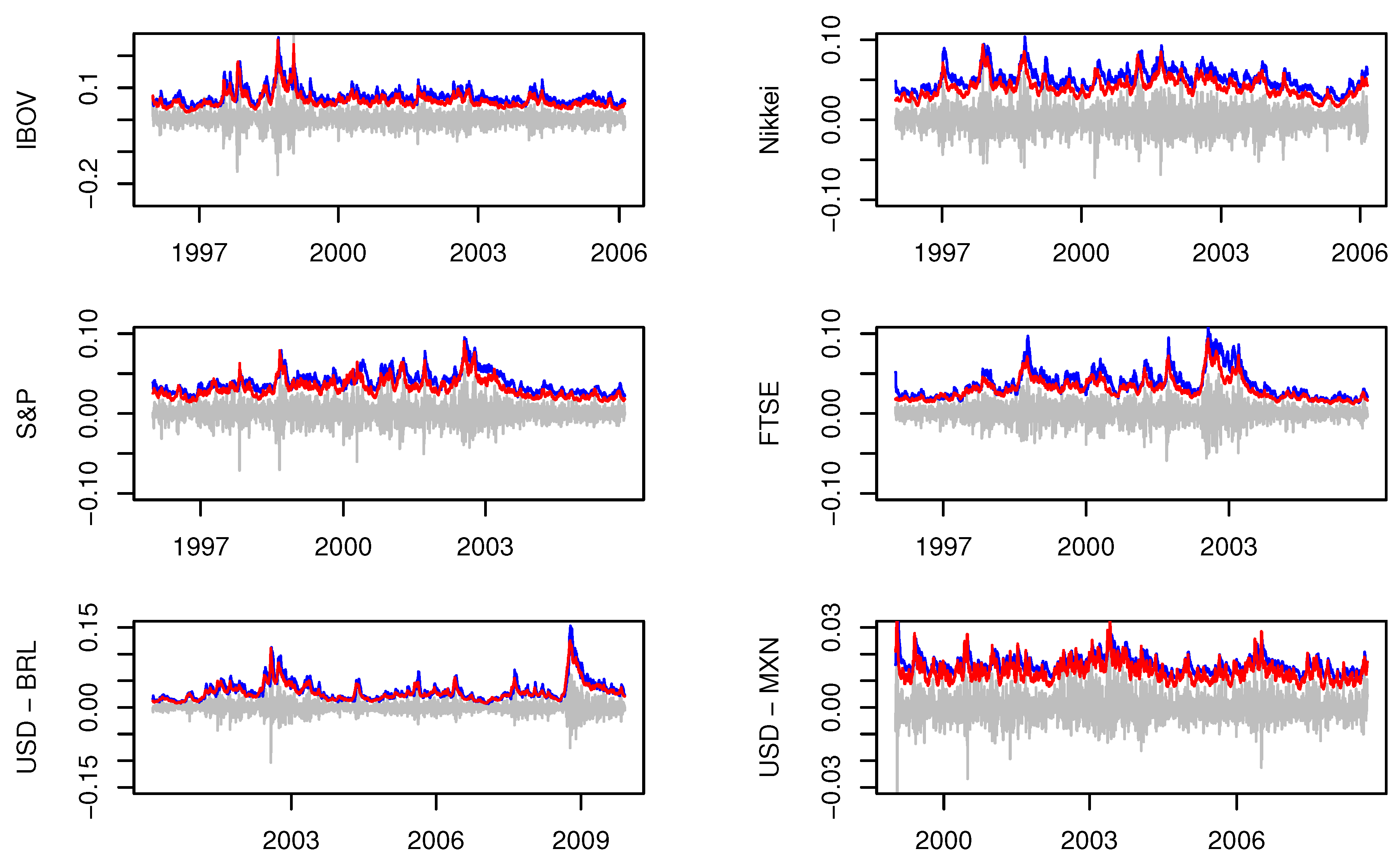
In Figure 1, we present a graph of the predicted volatility, , which was obtained from the first 2500 observations, and the estimates are presented in Table 3. As observed, the volatility of the proposed method mimics the variability of returns, with peaks associated with financial crisis episodes between 1996 and 2010. To name a few, we can observe an increase in volatility at the beginning of 1999 for IBOV, associated with the Brazilian currency crisis. In addition, we observed an increase in the volatility in 2008, which is associated with the subprime crisis.
We now discuss the results of a VaR backtesting exercise. We assessed the performance of the proposed method for both long and short positions. This is important because future volatilities in A-SV models present different behaviors when comparing negative and positive returns. As an example, consider the case of an asset for which its volatility has an increase after a fall in its price. The volatility of a seller will not increase after a loss in the same way as that of a buyer.
The backtesting exercise was performed with a rolling window with sample size of 2500. For each window, we estimated the model and computed the one-step ahead VaR forecast. Then, we evaluated the estimated VaRs using the tests of Kupiec (1995); Christoffersen (1998) and Christoffersen and Pelletier (2004).
The results of the backtesting exercise using the proposed method are presented in Table 4. Using , we found very good results for most of the series for both long and short positions. The exceptions are the 97.5%-VaR and 99%-VaR of a long position in the S&P, the 99%-VaR of a long position in the FTSE, and the 99%-VaR of a short position in the USD-MXN. For the other series, the proportion of violations is close to the nominal value (assessed by the Kupiec test), and for most cases, the violations are independent, assessed by the tests of Christoffersen (1998) and Christoffersen and Pelletier (2004), the latter abbreviated as CP. There are some situations where the p-values of CP tests are lower than 0.05: for example, the 99%-VaR of the long position in the IBOV and the S&P, and the 99%-VaR of the short position in the USD-MXN. Using , we also obtained good results, but these results are not as good compared with in terms of the proportions of violations and p-values of the tests. For instance, for most cases, the proportion of violations using is much closer to the nominal values compared to those obtained with .
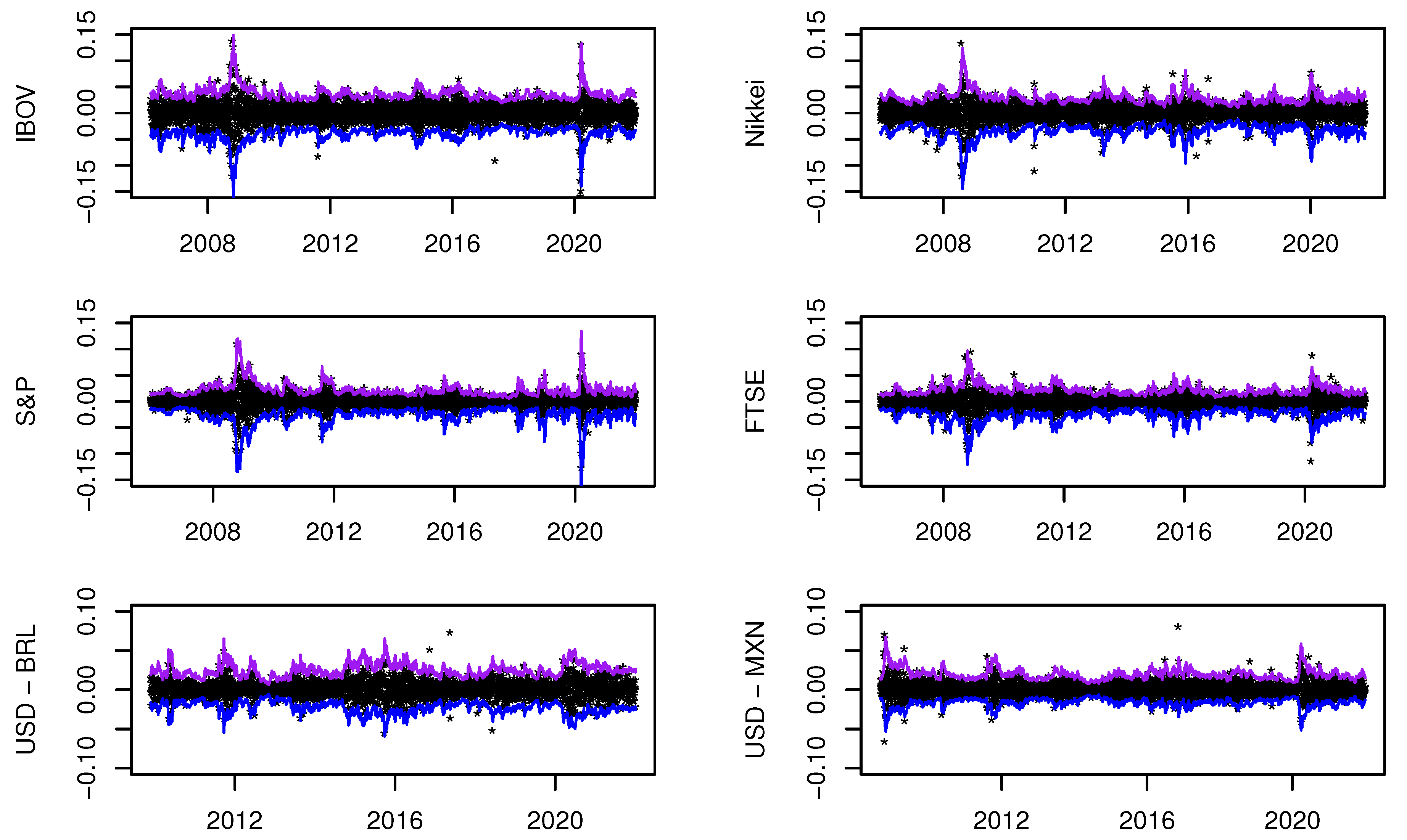
In Figure 2, we plot the predicted VaRs using our proposal. As observed, these values mimic the variability of returns. Additionally, we also observe an increase in VaR estimates during some crisis episodes during the period 2008–2021, e.g., the sub-prime crisis in 2008, the euro crisis in 2011, and the COVID-19 pandemic at the beginning of 2020.
We also estimated the time series using the stochvol method when 6. Using the first 2500 observations, we calculated the point parameter estimates of the posterior means. The results are shown in Table 3. Compared to the proposed method, the results are similar, with the exception of the USD-MXN series. In particular, according the point estimate and precision, the stochvol method accuses the presence of leverage for that series. In addition, in Figure 1, we present the stochvol estimates of , as described in Section 2.4. As can be seen, these estimates are very similar to those obtained when using the proposed method.
The backtesting results using the stochvol method are presented in Table 5. We observed better results using the proposal with than the stochvol method. For instance, excluding three cases (the 95%-VaR of a long position in the Nikkei, the 99%-VaR of a long position in the USD-BRL, and the 97.5%-VaR of a short position in the USD-BRL), the proportion of the violations of the proposal is much closer to the nominal values than those of the stochvol method.
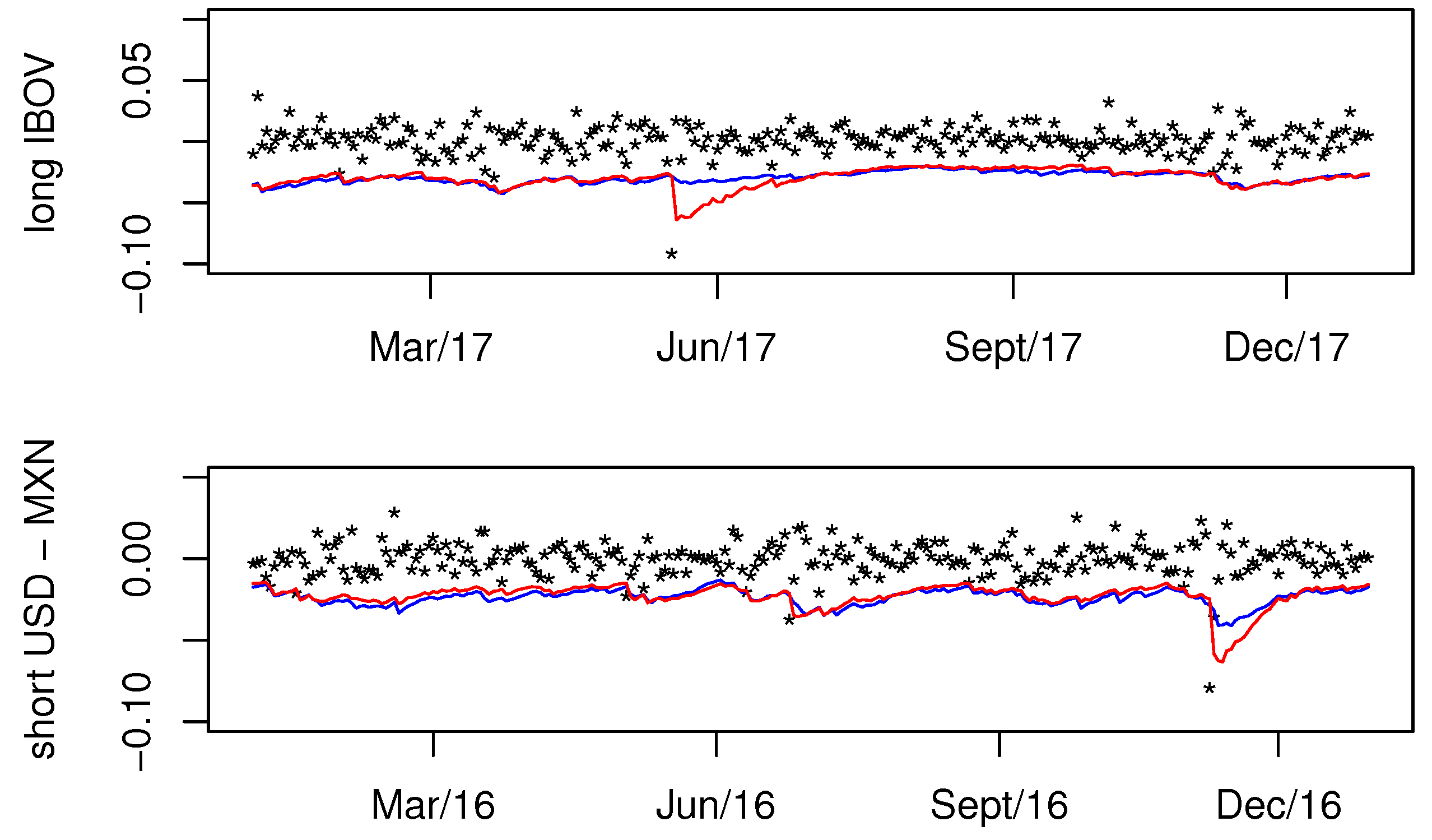
Although not shown, the behavior of predicted VaRs using stochvol is graphically similar with that obtained using the proposal. However, even though the volatilities of both methods are close most of the time, the stochvol method is affected more by outliers. This fact can clearly be observed for two selected situations shown in Figure 3. Here, we can see that the 99%-VaR of our proposal is more stable than stochvol even after extreme returns. This occurs for a long position in IBOV, after 17 May 2017, when news of a major scandal triggered a political crisis in Brazil during the administration of Michel Temer. The same happens for a short position in USD-MXN after 9 November 2016, when Donald Trump was elected the president of the USA.
5. Conclusions
In this study, we present a new method for the estimation of A-SV models that combines the framework of Shumway and Stoffer (2006, chp. 6) for SV models and the proposal of Omori et al. (2007) in order to approximate the density: .
The performance of the proposed method was assessed via Monte Carlo experiments. Overall, we obtained very good results in terms of point estimations.
In addition, the paper presents a procedure to forecast the value-at-risk for A-SV models. To evaluate the empirical performance of the proposal, an empirical study using stock market returns and FX returns is presented. The backtesting analysis of the VaR indicates that the proposed method is very good for both long and short positions. Hence, in practice, the estimation and VaR-forecasting procedures can be applied regardless of the direction of the position.
We compared our proposal with the method available in the stochvol package using simulated data and real-life data. The Monte Carlo experiments reveal that in terms of point estimations, these methods show similar results in several situations but, overall, the proposal provides better results for estimating , the stochvol method is better for estimating leverage parameter , and there is no clear winner for estimating . The empirical analysis evidenced that even though both methods showed similar VaR forecasts for most parts of the analyzed time series, the proposal exhibited a percentage of violations closer to the nominal VaR values and that is better for accounting for the influence of outliers.
Finally, it is important to stress that all routines for estimation and forecasting VaR can be executed within a few seconds7, which is a very important feature for practitioners. All codes are available upon request.
Author Contributions
Conceptualization, O.A. and M.Z.; methodology, O.A. and M.Z.; software, O.A.; validation, O.A. and M.Z., formal analysis, O.A. and M.Z.; data curation, O.A.; writing—original draft preparation, O.A.; writing—review and editing, O.A. and M.Z.; visualization, M.Z.; fundind acquisition, M.Z. All authors have read and agreed to the published version of the manuscript.
Funding
This research was funded by Fundação de Amparo à Pesquisa do Estado de São Paulo (FAPESP), grant number 2018/04654-9.
Data Availability Statement
No new data were created or analyzed in this study. Data sharing is not applicable to this article.
Acknowledgments
The second author acknowledges the financial support of FAPESP (grant 2018/04654-9) and both authors acknowledge the support of the Center for Applied Research in Econometrics, Finance, and Statistics (CAREFS).
Conflicts of Interest
No potential conflicts of interest are reported by the authors.
Appendix A
This appendix contains the derivation of the Kalman filter algorithm for the A-SV model.
Let be the information from time 1 to time t. We start by obtaining . From Equation (2), we have
where is calculated as
and by (12), we obtain
with .
On the other hand, let
Therefore,
The expressions for and depend on the joint distribution of and , which is conditional upon and . Thus,
since and are uncorrelated.
Therefore, the bivariate distribution of and conditional on and is given by
Now, we find as follows.
In turn, to obtain , consider
| 1 | In the ARCH/GARCH framework, models for accounting for the leverage effect include the EGARCH model of Nelson (1991) and the GJR model proposed by Glosten et al. (1993), among others. |
| 2 | The results for are qualitative similar and are available upon request |
| 3 | The total number of observations are as follows: 6419 for IBOV, 6543 for S&P 500, 6371 for Nikkei, 6565 for FTSE, 5533 for USD-BRL, and 5977 for USD-MXN. |
| 4 | We tested our method for both FX series in a different period compared to Asai and McAleer (2011). Since we did not obtain significant correlation parameter estimates even when using the stochvol method, the results are not reported here. |
| 5 | However, is significant using the stochvol method, and so we considered this time series in our analysis. |
| 6 | We tested the estimation when , but all degrees of freedom were higher than 30; thus, the results did not differ greatly from the Gaussian distribution. |
| 7 | As pointed out by a referee, the estimation process can be accelerated by using steady state expressions in the Kalman filter. This idea can be particularly fruitful for more complex models and deserves further investigation. |
References
- Abbara, Omar, and Mauricio Zevallos. 2019. A note on stochastic volatility model estimation. Brazilian Review of Finance 17: 22–32. [Google Scholar] [CrossRef] [Green Version]
- Abbara, Omar, and Mauricio Zevallos. 2022. Estimation and forecasting of long memory stochastic volatility models. Studies in Nonlinear Dynamics and Econometrics. [Google Scholar] [CrossRef]
- Asai, Manabu, and Michael McAleer. 2011. Alternative assymmetric stochastic volatility models. Econometric Reviews 30: 548–64. [Google Scholar] [CrossRef] [Green Version]
- Black, Fischer. 1976. Studies of stock price volatility changes. In Proceedings of the Business and Economics Section of the American Statistical Association. Washington, DC: American Statistical Association, pp. 177–81. [Google Scholar]
- Christoffersen, Peter. 1998. Evaluating interval forecasts. Symposium on Forecasting and Empirical Methods in Macroeconomics and Finance 39: 841–62. [Google Scholar] [CrossRef]
- Christoffersen, Peter, and Denis Pelletier. 2004. Backtesting value-at-risk: A duration-based approach. Journal of Financial Econometrics 2: 84–108. [Google Scholar] [CrossRef]
- Glosten, Lawrence R., Ravi Jagannathan, and David E. Runkle. 1993. On the relation between the expected value and the volatility of nominal excess return on stocks. Journal of Finance 48: 1779–801. [Google Scholar] [CrossRef]
- Harvey, Andrew C., and Neil Shephard. 1996. Estimation of an asymmetric stochastic volatility model for asset returns. Journal of Business and Economic Statistics 14: 429–34. [Google Scholar]
- Hosszejni, Darjus, and Gregor Kastner. 2021. Modeling univariate and multivariate stochastic volatility in r with stochvol and factorstochvol. Journal of Statistical Software 100: 1–34. [Google Scholar] [CrossRef]
- Jacquier, Eric, Nicholas G. Polson, and Peter E. Rossi. 2004. Bayesian analysis of stochastic volatility models with fat-tails and correlated errors. Journal of Econometrics 122: 185–212. [Google Scholar] [CrossRef]
- Jensen, Mark J., and John M. Maheu. 2010. Bayesian semiparametric stochastic volatility modeling. Journal of Econometrics 157: 306–16. [Google Scholar] [CrossRef] [Green Version]
- Jensen, Mark J., and John M. Maheu. 2014. Estimating a semiparametric asymmetric stochastic volatility model with a dirichlet process mixture. Journal of Econometrics 178: 523–38. [Google Scholar] [CrossRef] [Green Version]
- Kupiec, Paul. 1995. Techniques for verifying the accuracy of risk management models. Journal of Derivatives 3: 73–84. [Google Scholar] [CrossRef]
- Mao, Xiuping, Veronika Czellar, Esther Ruiz, and Helena Veiga. 2020. Asymmetric stochastic volatility models: Properties and particle filter-based simulated maximum likelihood estimation. Econometrics and Statistics 13: 84–105. [Google Scholar] [CrossRef]
- McAleer, Michael. 2014. Asymmetry and leverage in conditional volatility models. Econometrics 2: 145–50. [Google Scholar] [CrossRef] [Green Version]
- Nakajima, Jouchi, and Yasuhiro Omori. 2012. Stochastic volatility model with leverage and asymmetrically heavy-tailed error using gh skew student’s-t distribution. Computational Statistics and Data Analysis 56: 3690–704. [Google Scholar] [CrossRef]
- Nelson, Daniel. 1991. Conditional heteroskedasticity in asset returns: A new approach. Econometrica 59: 347–70. [Google Scholar] [CrossRef]
- Omori, Yasuhiro, Siddhartha Chib, Neil Shephard, and Jouchi Nakajima. 2007. Stochastic volatility with leverage: Fast and efficient likelihood inference. Journal of Econometrics 140: 425–49. [Google Scholar] [CrossRef] [Green Version]
- R Core Team. 2020. R: A Language and Environment for Statistical Computing. Vienna: R Foundation for Statistical Computing. [Google Scholar]
- Schäfers, Torben, and Long Teng. 2022. Asymmetric stochastic volatility models with threshold and time-dependent correlations. Studies in Nonlinear Dynamics and Econometrics. [Google Scholar] [CrossRef]
- Selçuk, Faruk. 2005. Asymmetric stochastic volatility in emerging markets. Applied Financial Econometrics 15: 867–74. [Google Scholar] [CrossRef]
- Shumway, Robert H., and David S. Stoffer. 2006. Time Series Analysis and Its Applications. New York: Springer. [Google Scholar]
- Takahashi, Makoto, Toshiaki Watanabe, and Yasuhiro Omori. 2021. Forecasting daily volatility of stock price index using daily returns and realized volatility. Econometrics and Statistics. [Google Scholar] [CrossRef]
- Taylor, Stephen John. 1982. Financial returns modelled by the product of two stochastic processes—A study of daily sugar prices, 1961–79. In Time Series Analysis: Theory and Practice. Edited by Oliver Duncan Anderson. North-Holland and New York: Elsevier, vol. 1, pp. 203–26. [Google Scholar]
- Taylor, Stephen John. 1994. Modelling stochastic volatility: A review and comparative study. Mathematical Finance 4: 183–204. [Google Scholar] [CrossRef]
- Yu, Jun. 2005. On leverage in a stochastic volatility model. Journal of Econometrics 127: 165–78. [Google Scholar] [CrossRef]
Figure 1.
Estimated volatilities. The gray line denotes the returns of the first 2500 observations of each series. The blue line denotes the predicted volatility of our proposal using , while the red line denotes the sample mean of the posterior sample of the volatility, obtained from stochvol. In these graphs, all volatilities are multiplied by 3.

Figure 2.
Backtesting results of the proposed method with . The blue line is the predicted 99%-VaR of a long position, while the purple line is the 99%-VaR of a short position (with change in sign).
Figure 2.
Backtesting results of the proposed method with . The blue line is the predicted 99%-VaR of a long position, while the purple line is the 99%-VaR of a short position (with change in sign).

Figure 3.
Comparison of VaR forecasting. The blue line is the forecast using the proposed method (with ) and the red line is the forecast obtained using stochvol. The graph at the top shows the backtesting of 1%-quantile for IBOV during 2017 and the graph at the bottom shows the 99%-quantile for USD-MXN during 2016.


Table 1.
Results of Monte Carlo experiments for the A-SV model ( and around −7.36). For each case, the bias, standard deviation (SD), and root mean square error (RMSE) of the estimates are presented. Results are based on 1000 replications of a time series of size .
Table 1.
Results of Monte Carlo experiments for the A-SV model ( and around −7.36). For each case, the bias, standard deviation (SD), and root mean square error (RMSE) of the estimates are presented. Results are based on 1000 replications of a time series of size .
| Proposal | Stochvol | ||||||||||||||
|---|---|---|---|---|---|---|---|---|---|---|---|---|---|---|---|
| Case 1 | Bias | −0.005 | 0.008 | −0.141 | 0.120 | −0.006 | 0.026 | 0.382 | 0.096 | −0.012 | 0.017 | −0.002 | 0.090 | ||
| SD | 0.023 | 0.039 | 0.077 | 0.164 | 0.034 | 0.041 | 0.202 | 0.186 | 0.017 | 0.024 | 0.059 | 0.068 | |||
| RMSE | 0.024 | 0.039 | 0.160 | 0.203 | 0.034 | 0.049 | 0.432 | 0.210 | 0.021 | 0.030 | 0.059 | 0.113 | |||
| Case 2 | Bias | −0.004 | −0.005 | −0.145 | 0.121 | −0.004 | 0.022 | 0.359 | 0.114 | −0.013 | 0.020 | −0.005 | 0.150 | ||
| SD | 0.016 | 0.030 | 0.067 | 0.137 | 0.025 | 0.033 | 0.205 | 0.152 | 0.013 | 0.020 | 0.050 | 0.049 | |||
| RMSE | 0.016 | 0.030 | 0.160 | 0.183 | 0.025 | 0.039 | 0.413 | 0.189 | 0.018 | 0.029 | 0.050 | 0.158 | |||
| Case 3 | Bias | −0.002 | 0.023 | −0.148 | −0.134 | −0.002 | 0.055 | 0.399 | −0.108 | −0.005 | 0.009 | 0.002 | −0.045 | ||
| SD | 0.012 | 0.036 | 0.106 | 0.080 | 0.012 | 0.037 | 0.139 | 0.087 | 0.011 | 0.025 | 0.095 | 0.057 | |||
| RMSE | 0.013 | 0.043 | 0.182 | 0.156 | 0.012 | 0.066 | 0.423 | 0.138 | 0.012 | 0.026 | 0.095 | 0.072 | |||
| Case 4 | , | Bias | −0.008 | 0.006 | −0.523 | 0.153 | −0.008 | 0.021 | 0.037 | 0.110 | −0.030 | 0.041 | −0.020 | 0.135 | |
| SD | 0.026 | 0.046 | 0.081 | 0.145 | 0.032 | 0.048 | 0.169 | 0.167 | 0.045 | 0.045 | 0.074 | 0.079 | |||
| RMSE | 0.028 | 0.046 | 0.529 | 0.211 | 0.033 | 0.052 | 0.173 | 0.200 | 0.054 | 0.061 | 0.077 | 0.156 | |||
| Case 5 | Bias | −0.006 | −0.013 | −0.526 | 0.165 | −0.005 | 0.011 | 0.021 | 0.126 | −0.023 | 0.038 | −0.027 | 0.214 | ||
| SD | 0.019 | 0.038 | 0.076 | 0.176 | 0.019 | 0.038 | 0.137 | 0.149 | 0.027 | 0.032 | 0.066 | 0.060 | |||
| RMSE | 0.020 | 0.040 | 0.532 | 0.241 | 0.020 | 0.039 | 0.139 | 0.195 | 0.035 | 0.050 | 0.072 | 0.222 | |||
| Case 6 | , | Bias | −0.003 | 0.015 | −0.529 | −0.163 | −0.003 | 0.042 | 0.034 | −0.124 | −0.009 | 0.019 | −0.014 | −0.062 | |
| SD | 0.013 | 0.039 | 0.113 | 0.083 | 0.013 | 0.041 | 0.238 | 0.096 | 0.014 | 0.033 | 0.107 | 0.066 | |||
| RMSE | 0.014 | 0.042 | 0.541 | 0.183 | 0.013 | 0.058 | 0.240 | 0.157 | 0.016 | 0.039 | 0.108 | 0.091 | |||
Table 2.
Results of Monte Carlo experiments for the A-SV model ( and around −7.36). For each case, the bias, standard deviation (SD), and root mean square error (RMSE) of the estimates are presented. Results are based on 1000 replications of a time series of size .
Table 2.
Results of Monte Carlo experiments for the A-SV model ( and around −7.36). For each case, the bias, standard deviation (SD), and root mean square error (RMSE) of the estimates are presented. Results are based on 1000 replications of a time series of size .
| Proposal | Stochvol | ||||||||||||||
|---|---|---|---|---|---|---|---|---|---|---|---|---|---|---|---|
| Case 1 | Bias | −0.002 | 0.022 | −0.119 | 0.149 | −0.002 | 0.052 | 0.402 | 0.133 | −0.002 | 0.007 | 0.007 | 0.078 | ||
| SD | 0.004 | 0.020 | 0.297 | 0.097 | 0.004 | 0.022 | 0.331 | 0.099 | 0.004 | 0.015 | 0.254 | 0.064 | |||
| RMSE | 0.004 | 0.030 | 0.320 | 0.178 | 0.004 | 0.056 | 0.521 | 0.166 | 0.004 | 0.017 | 0.254 | 0.100 | |||
| Case 2 | Bias | −0.001 | 0.007 | −0.150 | 0.174 | −0.001 | 0.043 | 0.327 | 0.175 | −0.002 | 0.008 | 0.024 | 0.123 | ||
| SD | 0.003 | 0.018 | 0.266 | 0.105 | 0.003 | 0.020 | 0.306 | 0.096 | 0.003 | 0.013 | 0.203 | 0.044 | |||
| RMSE | 0.004 | 0.020 | 0.305 | 0.204 | 0.004 | 0.047 | 0.448 | 0.200 | 0.004 | 0.015 | 0.204 | 0.131 | |||
| Case 3 | Bias | −0.001 | 0.043 | −0.065 | −0.151 | −0.001 | 0.087 | 0.419 | −0.137 | −0.002 | 0.005 | 0.025 | −0.040 | ||
| SD | 0.004 | 0.026 | 0.752 | 0.071 | 0.004 | 0.029 | 0.852 | 0.078 | 0.003 | 0.019 | 0.443 | 0.055 | |||
| RMSE | 0.004 | 0.051 | 0.755 | 0.167 | 0.004 | 0.092 | 0.949 | 0.157 | 0.004 | 0.020 | 0.444 | 0.068 | |||
| Case 4 | , | Bias | −0.002 | 0.014 | −0.522 | 0.190 | −0.002 | 0.039 | −0.001 | 0.158 | −0.003 | 0.010 | −0.007 | 0.105 | |
| SD | 0.004 | 0.022 | 0.275 | 0.102 | 0.004 | 0.025 | 0.370 | 0.111 | 0.004 | 0.018 | 0.260 | 0.072 | |||
| RMSE | 0.005 | 0.027 | 0.590 | 0.215 | 0.005 | 0.046 | 0.370 | 0.192 | 0.005 | 0.020 | 0.260 | 0.127 | |||
| Case 5 | Bias | −0.002 | −0.003 | −0.537 | 0.224 | −0.002 | 0.026 | −0.059 | 0.202 | −0.003 | 0.010 | −0.006 | 0.166 | ||
| SD | 0.004 | 0.022 | 0.252 | 0.125 | 0.004 | 0.024 | 0.364 | 0.119 | 0.004 | 0.016 | 0.216 | 0.050 | |||
| RMSE | 0.004 | 0.022 | 0.593 | 0.257 | 0.004 | 0.035 | 0.368 | 0.235 | 0.005 | 0.019 | 0.216 | 0.174 | |||
| Case 6 | , | Bias | −0.001 | 0.034 | −0.520 | −0.177 | −0.001 | 0.071 | 0.011 | −0.150 | −0.002 | 0.008 | −0.008 | −0.053 | |
| SD | 0.004 | 0.027 | 0.633 | 0.074 | 0.004 | 0.032 | 0.730 | 0.085 | 0.004 | 0.022 | 0.462 | 0.063 | |||
| RMSE | 0.004 | 0.043 | 0.819 | 0.191 | 0.004 | 0.078 | 0.730 | 0.172 | 0.004 | 0.023 | 0.462 | 0.083 | |||
Table 3.
Results of the estimation of the A-SV model for the real-life time series using the first 2500 observations. The standard errors and standard deviations for the proposal and stochvol methods are in parentheses.
Table 3.
Results of the estimation of the A-SV model for the real-life time series using the first 2500 observations. The standard errors and standard deviations for the proposal and stochvol methods are in parentheses.
| Proposal | Stochvol | ||||||||||||
|---|---|---|---|---|---|---|---|---|---|---|---|---|---|
| IBOV | Estimate | 0.975 | 0.168 | −7.950 | −0.386 | 0.968 | 0.224 | −7.431 | −0.413 | 0.956 | 0.214 | −7.850 | −0.471 |
| Std. error/Std. dev. | (0.010) | (0.034) | (0.172) | (0.118) | (0.011) | (0.041) | (0.165) | (0.113) | (0.010) | (0.025) | (0.095) | (0.058) | |
| Nikkei | Estimate | 0.982 | 0.136 | −8.811 | −0.345 | 0.984 | 0.157 | −8.254 | −0.380 | 0.971 | 0.165 | −8.727 | −0.463 |
| Std. error/Std. dev. | (0.008) | (0.029) | (0.191) | (0.155) | (0.007) | (0.032) | (0.206) | (0.162) | (0.007) | (0.020) | (0.111) | (0.063) | |
| S&P 500 | Estimate | 0.986 | 0.104 | −9.244 | −0.776 | 0.986 | 0.138 | −8.704 | −0.760 | 0.976 | 0.163 | −9.135 | −0.658 |
| Std. error/Std. dev. | (0.006) | (0.024) | (0.166) | (0.170) | (0.005) | (0.026) | (0.173) | (0.123) | (0.006) | (0.020) | (0.110) | (0.047) | |
| FTSE | Estimate | 0.987 | 0.137 | −9.222 | −0.728 | 0.986 | 0.178 | −8.744 | −0.752 | 0.987 | 0.135 | −9.265 | −0.627 |
| Std. error/Std. dev. | (0.004) | (0.022) | (0.219) | (0.136) | (0.004) | (0.025) | (0.208) | (0.105) | (0.003) | (0.015) | (0.174) | (0.058) | |
| USD-BRL | Estimate | 0.980 | 0.249 | −9.581 | 0.224 | 0.979 | 0.279 | −9.127 | 0.234 | 0.980 | 0.210 | −9.592 | 0.322 |
| Std. error/Std. dev. | (0.007) | (0.039) | (0.299) | (0.104) | (0.007) | (0.041) | (0.277) | (0.111) | (0.005) | (0.019) | (0.211) | (0.062) | |
| USD-MXN | Estimate | 0.968 | 0.143 | −11.037 | 0.163 | 0.967 | 0.164 | −10.463 | 0.118 | 0.862 | 0.354 | −10.926 | 0.363 |
| Std. error/Std. dev. | (0.018) | (0.046) | (0.135) | (0.170) | (0.018) | (0.052) | (0.155) | (0.191) | (0.038) | (0.059) | (0.060) | (0.054) | |
Table 4.
Backtesting results using the proposal.
| Asset | Stat/Test | Long Position | Short Position | Long Position | Short Position | ||||||||
|---|---|---|---|---|---|---|---|---|---|---|---|---|---|
| IBOV | Proportion | 0.012 | 0.024 | 0.048 | 0.047 | 0.026 | 0.011 | 0.011 | 0.024 | 0.048 | 0.046 | 0.025 | 0.010 |
| Kupiec | 0.287 | 0.608 | 0.558 | 0.332 | 0.682 | 0.656 | 0.547 | 0.608 | 0.558 | 0.301 | 0.920 | 0.773 | |
| Christoffersen | 0.483 | 0.082 | 0.513 | 0.385 | 0.899 | 0.574 | 0.663 | 0.082 | 0.795 | 0.380 | 0.959 | 0.622 | |
| Christoffersen-Pelletier | 0.029 | 0.045 | 0.421 | 0.516 | 0.699 | 0.708 | 0.029 | 0.015 | 0.668 | 0.064 | 0.953 | 0.428 | |
| Nikkei | Proportion | 0.014 | 0.029 | 0.052 | 0.051 | 0.026 | 0.013 | 0.012 | 0.029 | 0.052 | 0.050 | 0.026 | 0.012 |
| Kupiec | 0.029 | 0.126 | 0.489 | 0.744 | 0.666 | 0.110 | 0.195 | 0.152 | 0.536 | 0.909 | 0.741 | 0.322 | |
| Christoffersen | 0.042 | 0.021 | 0.459 | 0.910 | 0.834 | 0.253 | 0.140 | 0.022 | 0.612 | 0.977 | 0.878 | 0.513 | |
| Christoffersen-Pelletier | 0.016 | 0.003 | 0.115 | 0.075 | 0.718 | 0.167 | 0.030 | 0.135 | 0.252 | 0.008 | 0.470 | 0.133 | |
| S&P 500 | Proportion | 0.017 | 0.034 | 0.056 | 0.052 | 0.026 | 0.013 | 0.016 | 0.032 | 0.055 | 0.050 | 0.025 | 0.011 |
| Kupiec | 0.000 | 0.000 | 0.105 | 0.481 | 0.769 | 0.080 | 0.000 | 0.009 | 0.180 | 0.894 | 0.994 | 0.389 | |
| Christoffersen | 0.000 | 0.002 | 0.266 | 0.029 | 0.868 | 0.201 | 0.000 | 0.022 | 0.407 | 0.065 | 0.956 | 0.406 | |
| Christoffersen-Pelletier | 0.001 | 0.047 | 0.099 | 0.010 | 0.914 | 0.432 | 0.001 | 0.113 | 0.083 | 0.000 | 0.329 | 0.247 | |
| FTSE | Proportion | 0.014 | 0.031 | 0.050 | 0.053 | 0.028 | 0.013 | 0.013 | 0.028 | 0.049 | 0.052 | 0.025 | 0.013 |
| Kupiec | 0.022 | 0.030 | 0.900 | 0.443 | 0.188 | 0.086 | 0.045 | 0.261 | 0.815 | 0.579 | 0.970 | 0.117 | |
| Christoffersen | 0.036 | 0.014 | 0.071 | 0.025 | 0.015 | 0.117 | 0.128 | 0.031 | 0.157 | 0.002 | 0.072 | 0.153 | |
| Christoffersen-Pelletier | 0.461 | 0.236 | 0.478 | 0.000 | 0.027 | 0.895 | 0.916 | 0.406 | 0.756 | 0.000 | 0.057 | 0.778 | |
| USD-BRL | Proportion | 0.012 | 0.026 | 0.054 | 0.048 | 0.023 | 0.010 | 0.011 | 0.025 | 0.054 | 0.049 | 0.023 | 0.010 |
| Kupiec | 0.405 | 0.801 | 0.310 | 0.697 | 0.420 | 0.952 | 0.511 | 0.923 | 0.272 | 0.760 | 0.493 | 0.903 | |
| Christoffersen | 0.470 | 0.773 | 0.230 | 0.927 | 0.639 | 0.740 | 0.548 | 0.990 | 0.326 | 0.549 | 0.686 | 0.721 | |
| Christoffersen-Pelletier | 0.679 | 0.094 | 0.038 | 0.956 | 0.482 | 0.553 | 0.661 | 0.230 | 0.013 | 0.686 | 0.451 | 0.492 | |
| USD-MXN | Proportion | 0.009 | 0.026 | 0.050 | 0.054 | 0.027 | 0.013 | 0.010 | 0.026 | 0.050 | 0.053 | 0.025 | 0.013 |
| Kupiec | 0.632 | 0.660 | 0.929 | 0.312 | 0.448 | 0.131 | 0.895 | 0.585 | 0.929 | 0.390 | 0.994 | 0.095 | |
| Christoffersen | 0.662 | 0.531 | 0.343 | 0.016 | 0.043 | 0.020 | 0.709 | 0.071 | 0.343 | 0.288 | 0.239 | 0.018 | |
| Christoffersen-Pelletier | 0.990 | 0.952 | 0.134 | 0.085 | 0.002 | 0.001 | 0.364 | 0.352 | 0.025 | 0.384 | 0.009 | 0.035 | |
Table 5.
Backtesting results using stochvol.
| Asset | Stat/Test | Long Position | Short Position | ||||
|---|---|---|---|---|---|---|---|
| IBOV | Prop | 0.011 | 0.024 | 0.043 | 0.038 | 0.018 | 0.008 |
| Kupiec | 0.547 | 0.760 | 0.052 | 0.000 | 0.004 | 0.124 | |
| Christoffersen | 0.518 | 0.934 | 0.149 | 0.002 | 0.014 | 0.243 | |
| Christoffersen-Pelletier | 0.718 | 0.990 | 0.529 | 0.356 | 0.284 | 0.568 | |
| Nikkei | Prop | 0.014 | 0.032 | 0.051 | 0.043 | 0.016 | 0.005 |
| Kupiec | 0.009 | 0.013 | 0.800 | 0.045 | 0.000 | 0.000 | |
| Christoffersen | 0.017 | 0.044 | 0.968 | 0.134 | 0.001 | 0.000 | |
| Christoffersen-Pelletier | 0.648 | 0.950 | 0.476 | 0.687 | 0.027 | 0.261 | |
| S&P 500 | Prop | 0.019 | 0.037 | 0.060 | 0.044 | 0.017 | 0.005 |
| Kupiec | 0.000 | 0.000 | 0.003 | 0.089 | 0.001 | 0.001 | |
| Christoffersen | 0.000 | 0.000 | 0.005 | 0.120 | 0.001 | 0.005 | |
| Christoffersen-Pelletier | 0.660 | 0.878 | 0.061 | 0.274 | 0.468 | 0.786 | |
| FTSE | Prop | 0.016 | 0.035 | 0.057 | 0.040 | 0.017 | 0.006 |
| Kupiec | 0.000 | 0.000 | 0.059 | 0.002 | 0.001 | 0.008 | |
| Christoffersen | 0.000 | 0.000 | 0.162 | 0.000 | 0.001 | 0.025 | |
| Christoffersen-Pelletier | 0.053 | 0.148 | 0.123 | 0.005 | 0.944 | 0.282 | |
| USD-BRL | Prop | 0.009 | 0.017 | 0.044 | 0.054 | 0.026 | 0.010 |
| Kupiec | 0.536 | 0.005 | 0.134 | 0.310 | 0.630 | 0.952 | |
| Christoffersen | 0.415 | 0.004 | 0.009 | 0.571 | 0.888 | 0.740 | |
| Christoffersen-Pelletier | 0.412 | 0.905 | 0.479 | 0.394 | 0.749 | 0.412 | |
| USD-MXN | Prop | 0.008 | 0.020 | 0.043 | 0.067 | 0.034 | 0.018 |
| Kupiec | 0.311 | 0.033 | 0.069 | 0.000 | 0.001 | 0.001 | |
| Christoffersen | 0.469 | 0.026 | 0.102 | 0.001 | 0.002 | 0.001 | |
| Christoffersen-Pelletier | 0.899 | 0.281 | 0.194 | 0.018 | 0.529 | 0.091 | |
Disclaimer/Publisher’s Note: The statements, opinions and data contained in all publications are solely those of the individual author(s) and contributor(s) and not of MDPI and/or the editor(s). MDPI and/or the editor(s) disclaim responsibility for any injury to people or property resulting from any ideas, methods, instructions or products referred to in the content. |
© 2022 by the authors. Licensee MDPI, Basel, Switzerland. This article is an open access article distributed under the terms and conditions of the Creative Commons Attribution (CC BY) license (https://creativecommons.org/licenses/by/4.0/).
Share and Cite
MDPI and ACS Style
Abbara, O.; Zevallos, M. Maximum Likelihood Inference for Asymmetric Stochastic Volatility Models. Econometrics 2023, 11, 1. https://doi.org/10.3390/econometrics11010001
AMA Style
Abbara O, Zevallos M. Maximum Likelihood Inference for Asymmetric Stochastic Volatility Models. Econometrics. 2023; 11(1):1. https://doi.org/10.3390/econometrics11010001
Chicago/Turabian StyleAbbara, Omar, and Mauricio Zevallos. 2023. "Maximum Likelihood Inference for Asymmetric Stochastic Volatility Models" Econometrics 11, no. 1: 1. https://doi.org/10.3390/econometrics11010001
Note that from the first issue of 2016, this journal uses article numbers instead of page numbers. See further details here.