Energy-Efficient Relay Tracking and Predicting Movement Patterns with Multiple Mobile Camera Sensors

Abstract

Camera sensor networks (CSN) have been widely used in different applications such as large building monitoring, social security, and target tracking. With advances in visual and actuator sensor technology in the last few years, deploying mobile cameras in CSN has become a possible and efficient solution for many CSN applications. However, mobile camera sensor networks still face several issues, such as limited sensing range, the optimal deployment of camera sensors, and the energy consumption of the camera sensors. Therefore, mobile cameras should cooperate in order to improve the overall performance in terms of enhancing the tracking quality, reducing the moving distance, and reducing the energy consumed. In this paper, we propose a movement prediction algorithm to trace the moving object based on a cooperative relay tracking mechanism. In the proposed approach, the future path of the target is predicted using a pattern recognition algorithm by applying data mining to the past movement records of the target. The efficiency of the proposed algorithms is validated and compared with another related algorithm. Simulation results have shown that the proposed algorithm guarantees the continuous tracking of the object, and its performance outperforms the other algorithms in terms of reducing the total moving distance of cameras and reducing energy consumption levels. For example, in terms of the total moving distance of the cameras, the proposed approach reduces the distance by 4.6% to 15.2% compared with the other protocols that do not use prediction.

1. Introduction

In the last few years, the emergence of Internet of Things (IoT) applications has paved the way for enhancing the services provided to users in indoor smart buildings like airports, hospitals, and supermarkets [1]. In such environments that emphasize human needs, a person’s location is critical information. It has the potential to improve a wide range of services and applications, including energy management, smart HVAC controls, tracking, navigation, healthcare, and emergency response [2,3,4,5,6]. For example, even a one-minute reduction in emergency response time due to improved localization accuracy can save nearly 10,000 lives each year in the United States alone [7]. Because most people spend the majority of their time indoors, there is a strong emphasis on improving indoor localization, as the normal GPS cannot be utilized owing to signal interference and reflection, which obstruct the line of sight to reference satellites. As a result, researchers are actively looking for accurate and widely available alternatives to GPS for indoor localization. Different technologies have been proposed for indoor localization, including magnetic fields, WiFi, Bluetooth, and hybrid sensor fusion [8,9,10]. However, compared with the previous techniques, camera sensor networks (CSN), which are composed of distributed camera sensor nodes, require no collaboration from the object being tracked. Moreover, CSN-based object tracking techniques have more advantages as they are robust to failures and they utilize the communication infrastructure in the environment more efficiently [11].

This paper concentrates on the security and safety of individuals and facilities as a service provided by institutions. To attain this service, video surveillance is used as a monitoring tool [12]. Over time, video surveillance records the motions of any moving objects in a certain area. One of the most important functions of video surveillance is to detect and assist in the investigation of illegal activities. When utilized in advance of questionable actions, it may also serve as a deterrent [13]. Because of that, camera sensor networks have attracted wide research attention over the past few years. Consequently, camera sensor networks have been utilized in a wide range of applications, including area monitoring and surveillance. Camera sensor networks are employed as a tool in object identification and tracking tasks. Object detection determines when an object will appear inside the camera’s visual range. On the other hand, multiple camera sensors are employed to constantly monitor the object as it passes across the region to ensure continuous monitoring.

For all sensors, a camera’s position in a network of cameras is critical to its performance. A basic configuration for each site might include the number of cameras needed to cover the whole area while maintaining relationships with other nearby cameras, the viewing range of each camera, and which regions are covered by a particular camera. The camera sensor network’s most important feature is its ability to monitor suspicious objects by moving the cameras around the network’s perimeter. However, the overlap between the neighboring cameras resulted in a waste of energy and duplicated recorded images. As a result, we require more information that may be utilized to identify the camera that should be moved to a specific location or to switch between cameras as the object moves to reduce the total energy consumed. However, utilizing the traditional tracking and monitoring method [14] still has security issues, such as employing fixed positions for cameras. Increased camera deployment is required to guarantee coverage of the whole region being monitored. In contrast, if cameras are placed in a fixed position, the target can use the blind spot that is not covered by the cameras, allowing him to deliberately avoid the cameras while committing crimes [15]. In most applications, the applied analysis of moving objects reveals that the behavior of object movement is not totally random and is generally dependent on particular occurrences. The observation of animals like birds moving generally forms an orderly cluster during periods of migration to seek food. Data mining approaches for wireless sensor networks (WSNs) provide numerous benefits in terms of detection and energy savings. As part of our efforts to improve tracking accuracy, we will observe and identify the relevant rules from the object’s prior movement pattern and compare them with the movement pattern of the past observation to forecast its upcoming position. Consequently, the demand for energy-efficient systems for tracking objects has risen. To choose the lowest number of sensors to be in active mode, we present a tracking method that employs both relay tracking between cameras and the prediction pattern of object movement.

Existing research on this topic focuses on avoiding blind areas [16], enhancing detection probability [17], or creating routes for mobile cameras [18]. However, in this paper, cooperative relay tracking between mobile camera sensors is developed by including the prediction of object movement in the tracking process. The primary idea of the relay tracking algorithm is to schedule the mobile camera sensors to follow the target and select the cameras with the shortest moving distance that will follow the target to ensure continuous monitoring of the target. The target movement is based on the Markov Chain Monte Carlo model probability [19]. Using data mining techniques, we aim to develop an energy-efficient relay tracking algorithm to identify the movement of a target. To conserve energy, only a limited number of cameras will be utilized to monitor a single target. Figure 1 shows a simple scenario of the target and the camera’s movement in a mall. As illustrated in the figure, multiple camera sensors may be used to track any moving object in the mall area.

As we can see, in this scenario, the target is moving from one shop to another. His future path is illustrated by the red line in the figure. Whenever the target is moving, the camera closest to it is also moving to keep up with the target’s activities. When the target passes across an intersection point where more than one camera is available, the total moving distance of cameras can be reduced by using a camera relay. Based on the target’s prior movements, the prediction pattern is used to predict the target’s upcoming movement. When the target moves, only the chosen camera will be active, and its movement is determined by the cooperative relay algorithm, which is utilized to reduce the total movement distance of cameras.

As the demand for information on building power consumption grows, it’s important to explore cost-effective ways to collect, store, and visualize this data. Current building management solutions are costly and difficult to implement in small and medium-sized buildings that lack intelligence. Several articles proposed various techniques, but none of them examined the prediction of target movement in the relay monitoring of the camera’s movement. In this paper, we examine the notion of activating and scheduling cameras in CSN by predicting the target’s future route based on the determined frequency of movement patterns. Our main contribution in this paper is threefold, as follows:

• We implemented and enhanced the mobile cooperative relay algorithm [20] to demonstrate that it reduces the total moving distance of cameras and provides efficient monitoring time.
• We consider a single target problem and apply path prediction based on data mining.
• Cooperative relay tracking is used in cooperation with object movement prediction to obtain the shortest possible movement distance between camera sensors while also saving energy.

The rest of this paper is organized as follows: Section 2 reviews the related work. Section 3 discusses the proposed approach. The simulation results are illustrated in Section 4, and the paper is concluded in Section 5.

2. Related Work

Surveillance systems play major roles in infrastructure monitoring for the security of things, places, and people. In order to replace outdated surveillance cameras, new technologies with surveillance capabilities are being created. The main challenge in a surveillance system is constantly monitoring a moving object while also trying to conserve energy by placing each camera sensor in the most efficient location possible, which is not always possible. In this context, Gao et al. [21] proposed a full-view barrier-covered model that works with a randomly deployed WMSN that drives camera sensors to create a full-view covered barrier. In order to obtain full coverage, they analyzed the needed number of camera sensors for their system and experimented hwith different parameters. The authors utilized two centralized methods (S-Dijkstra, S-Thorup). The authors prove that their technique can guarantee full view coverage while using fewer camera sensors.

The authors of [22] attempted to address the object tracking problem by employing real-time tracking that handled position and feature vectors that would be extracted for the area-of-interest object in two frames. They utilized the Euclidean distance to evaluate the extracted features between the first frame feature vectors and the second frame, trying to identify the minimum distance between the two frames. However, the feature comparison has difficulty encoding the changes that came from the long-term view because of the changes in the view angle and the light settings.

The authors of [23] introduced DROP, a novel framework for monitoring multiple objects. In this framework, objects are tracked by calculating the affinity between the previous tracking trajectory and the detection at the present video frame by creating several measurements such as appearance and motion and then merging them based on confidence. The authors employed a lightweight convolutional neural network to extract characteristics from observed individuals. This network can tackle the re-tracking problem by raising and learning the affinity of the appearance features of the same object in multiple frames.

In [24], the authors utilize an adaptive model of every object that is compatible with any adaptively updated feature. They observe the long-term perspective change online. The authors also designed re-identification schemes to handle closer targets who share a similar appearance. All these algorithms are based on a fixed tracking model. The problem with selecting a fixed place for the camera sensor is that it is easy for criminal suspects to avoid cameras by walking through blind spots where the camera cannot capture them. To resolve the issue of the cameras being fixed in one place by making the routing protocol adaptable to the change in network topology in advance, Ref. [25] presented a hole recovery method that improves the routing protocol.

With the growth of deep learning, multi-object tracking systems that employ deep neural networks partition distinct functional modules into many networks and train them individually on certain tasks. As a result of all of the modules being used directly, tracking will be poor, and there will be incompatibility concerns. As a result, the authors of [26] developed a novel approach that combines object regression across frames for a single model and exploits features to improve the coherence between diverse functional modules of multi-object tracking. The results show that the proposed approach achieves state-of-the-art performance. The majority of the current research focuses on the deployment of the camera sensor while attempting to accomplish effective monitoring of the movement path [27]. The authors of [28] suggested a control algorithm that employs local information exchange for monitoring trains, whereas the authors of [29] attempted to achieve high detection probability by predicting the target’s future position and then directing the camera sensors. Many approaches have been presented to offer precise camera calibration, such as [30,31], which uses a collection of reference points with known locations. Moreover, the authors in [32] presented a sensor network approach that relies on estimating the outer parameters of cameras, whereas [33] proposed a distributed technique that relies on calibrating networked cameras. Examples include a solution described by [34] to solve object tracking and camera calibration difficulties, such that when tracking objects, a camera’s cooperation is required. It’s possible to use a calibrated camera system for object tracking by using a system like [35].

However, none of the papers discussed above have considered the prediction of target movement in the relay tracking of the cameras movements. In this paper, we investigate the idea of activating and scheduling the cameras in CSN by predicting the future route of the target using the calculated frequency of the movement patterns.

3. Proposed Approach

As a result of the constant operation of camera sensor nodes in many existing monitor systems, a significant amount of energy is wasted. The proposed approach addresses this problem and presents a tracking algorithm by scheduling camera sensor nodes in active-sleep states efficiently, therefore reducing the energy consumption levels. The proposed approach employs a cooperative relay tracking algorithm to construct a movement schedule of the camera sensors to determine which camera should move and stay active and which camera should take over the monitoring operation by predicting the future route of the moving object. The proposed approach is divided into three stages:

• Prediction of an object’s future movement to activate only the camera sensor nodes required to follow the object;
• A wake-up technique that determines which nodes and when they should be activated based on some heuristics that take both energy and performance into account;
• A recovery mechanism that is activated only when the camera sensors fail to predict the object’s future path.

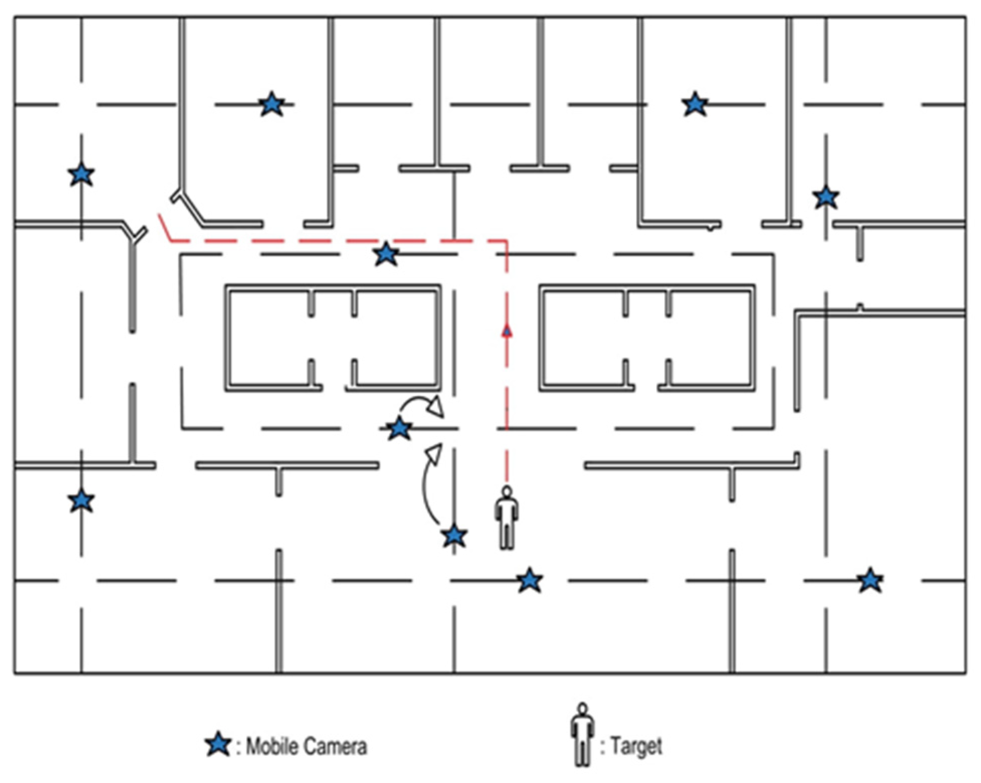
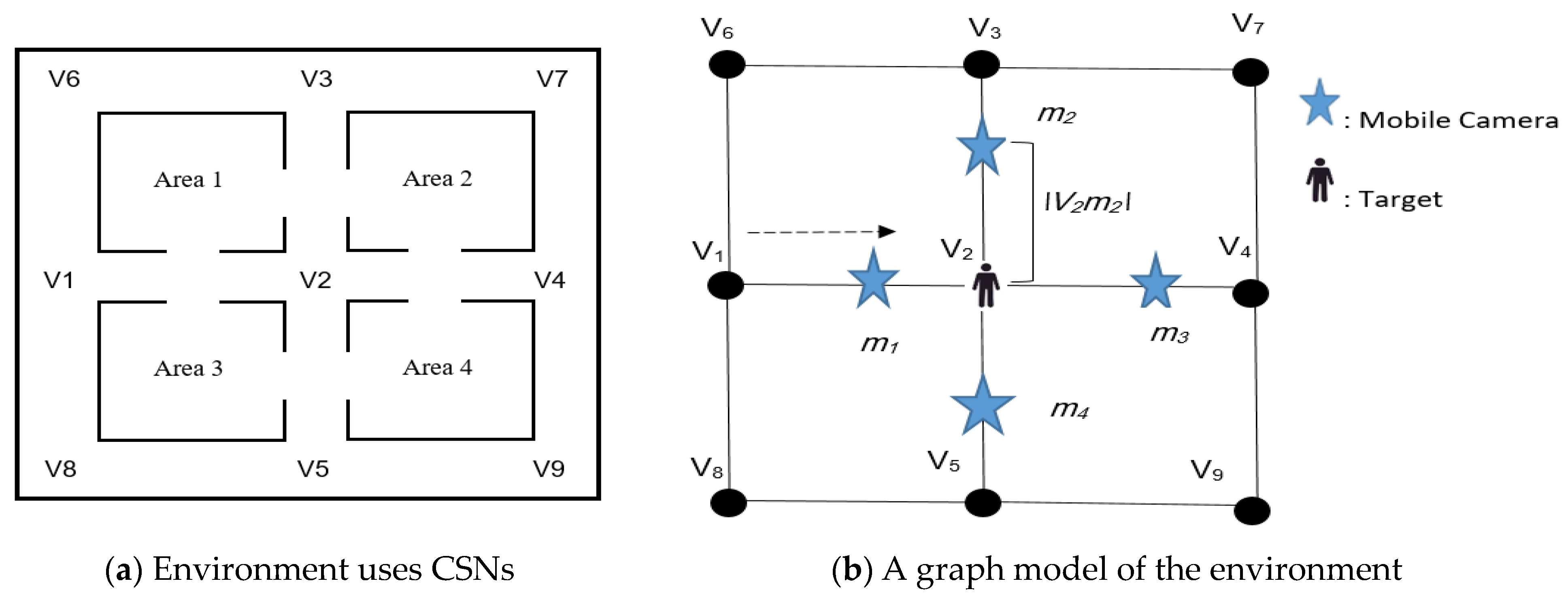
3.1. Tracking Problem Definition

Assume CN mobile camera sensors are deployed randomly in an environment, such as a building or an area composed of streets that intersect with each other. Suppose, as shown in Figure 2a, that a target navigates around some areas in the environment. This situation can be modeled as a graph (G = V, E), where V = {V₁, V₂, …, V_n} represents the set of vertices in G and E = {E₁, E₂, …, E_m} represents the set of edges, as shown in Figure 2b. Each vertex is an intersection point between two or more paths in the given environment. Every camera has a visual range denoted as v. A tracking camera records the movement distance Td of the target as it travels randomly from vertex to vertex. It is assumed that each camera knows the graph topology and records the target location when the target is within its visual range. As the target moves from one vertex to another, several camera sensors will hold on to the path. Finding the required number of mobile camera sensors in order to reduce the cost of tracking the target is a critical problem in CSNs. Since moving and activating unnecessary camera sensors in order to be ready to track the target will result in consuming some of the energy of these cameras. For example, when the target in Figure 2b moves from V₁ to V₃, without any kind of cooperative relay tracking mechanism, all three cameras (m₂, m₃, and m₄) will be activated and ready to start tracking the target when it reaches vertex V₂. However, in the case of predicting the target’s future direction, only some cameras will be needed to monitor the target, and the other cameras should be set in a sleep state.

Example: As shown in Figure 2, assume the target is moving from V₁ toward V₃. Assume the following distances: X₁₂ = 120 m (the distance between V₁ and V₂), X₂₃ = 100 m (the distance between V₂ and V₃), X₂₄ = 120 m (the distance between V₂ and V₄), X₂₅ = 100 m (the distance between V₂ and V₅), d₂₁ = |V_2m1| = 10 m (the distance between V₂ and m₁), d₂₂ = |V_2m2| = 20 m (the distance between V₂ and m₂), and d₂₃ = |V_2m3| = 15 m (the distance between V₂ and m₃), and d₂₄ = |V_2m4| = 20 m (the distance between V₂ and m₄). Assume the visual range of camera sensors is 30 m. There are three methods for scheduling the camera sensors to track the target. The first one is to schedule m₂ to vertex V₂ to replace m₁. In this case, the total distance of moving the camera sensors will be 150 m (120 − 60 + 20 + 100 − 30). The second choice is to schedule m₃ to vertex V₂. In this case, the total distance of moving the camera sensors will be 115 m (120 − 60 + 15 + 100 − 20 − 30). The third choice is to schedule m₄ to vertex V₂. In this case, the total distance of moving the camera sensor will be 120 m (120 − 60 + 20 + 100 − 20 − 30). Thus, the second method has the shortest distance among the three choices.

The problem can be modeled as a linear programming model. Assume a target moves from a starting vertex vs. = V₁ to a final vertex V_f = V_m through a sequence of vertices vs. = V₁, V₂, V₃, …, V_m = V_f. Let Td be the total distance between vs. and V_f. Assume X_ij is the distance between V_i and V_j. Let CN be the number of camera sensors that should be activated to track the target along all the paths from vs. to V_f. Assume that di is the total distance that a set of activated camera sensors will move when the target reaches the vertex V_i. Then, the objective of the problem is:

Minimize

$${\displaystyle \sum }_{i=2}^m{d}_i$$

(1)

Subject to

$$T_d\le {\displaystyle \sum }_{i=1}^m{X}_{ij} , 1\le j\le m, i\ne j$$

(2)

$$m\le CN$$

(3)

The objective function in Equation (1) is to minimize the total distance that the activated camera sensors will move. Constraint (2) indicates that the total distance that the target will move should be less than or equal to the total distance between vs. and V_f. Constraint (3) indicates that the number of activated camera sensors should be at least m, assuming there is at least one camera between any two vertices. However, the cooperative relay tracking with multiple mobile camera sensors problem is NP-hard, as was proved in [20].

3.2. Relay Tracking Algorithm

According to Figure 2, the target is moving from V₁ to V₃ and will select the next camera for monitoring. In order to reschedule the camera sensor, we must consider the following scenarios: The first one is when a single camera can only be used if the target is moving and no other cameras are available to be used to follow the target’s progress on the future route line. For example, in Figure 2b, suppose that there is only one camera, which is m₁. Using Equation (4), the total distance can be computed as follows:

$$T_d=X_1+X_2-v$$

(4)

where X₁ and X₂ represent the distance between V₁ and V₂ and V₂ and V₃, respectively, and v represents the camera’s visual range. As for the second scenario, if there is another camera in the current path line, we will not move it to avoid incurring additional distance costs. Another camera on the future path is the third scenario. Suppose there are two cameras, m₁, which is the camera that currently follows the target, and m₂, which is the camera on the future route. In this case, the reduced distance is calculated as follows:

$$\mathsf{\Delta }=\{\begin{array}{l}v-2\left|v_2{m}_2\right| , v\le y\\ y-2\left|v_2{m}_2\right| , v>y\end{array}$$

(5)

where ∆ represents the reduced distance, v is the camera’s visual range, and y is the distance between V₂ and the moving target, and this will be satisfied if this meets the following equation:

$$\{\begin{array}{l}2\left|v_2{m}_2\right|<v\le y\\ 2\left|v_2{m}_2\right|<y<v\end{array}$$

(6)

The last scenario is that if we have two cameras, m₁, which is the camera that currently follows the target, and a camera in V₂V₅, like m₄, as shown in Figure 2b, which is not the future selected path, in this case, the reduced distance that will apply will be calculated using Equation (7):

$$\mathsf{\Delta }=\{\begin{array}{c}2v-2\left|v_2{m}_2\right| , v\le y\\ y+v-2\left|v_2{m}_2\right| ,v>y\end{array}$$

(7)

And this will be applied only if Equation (8) is satisfied:

$$\{\begin{array}{c}\left|v_2{m}_2\right|<2, y\ge v\\ \left|v_2{m}_2\right|<v, y<v\end{array}$$

(8)

To reschedule the camera sensors, we will calculate the expected value for each camera, including the current processing, and then select the camera that has the maximum value to replace the current one. Let ηVi Vj represent the movable probability of each edge. In light of [24]’s analysis, any camera can be chosen. Therefore, we will go with the one that will offer us the maximum reduced distance, which means that it will give us the shortest moving distance. The following equation will be applied to every camera near the target:

$$Exp={\mathsf{\eta }}_{V_i{V}_j}\times {\mathsf{\Delta }}_1+\left(1-{\mathsf{\eta }}_{V_i{V}_j}\right)\times {\mathsf{\Delta }}_2$$

(9)

The pseudo-code of the movement pattern generation and cooperative relay algorithm for a single target is shown in Algorithm 1. One of the two scenarios is if the target moves and the next vertex does not contain a camera sensor. Either a new camera is required to cover the region, or the existing camera, which is currently moving, continues to monitor until it reaches the next vertex. The selection of the next moving camera is based on the maximum expected value, so that the camera with the highest value will move to start monitoring. At the end of each step, we will update the states of the vertex and edge. However, the current monitoring camera will keep recording if there is no satisfactory camera. The second case is that future paths will have camera sensors, so they will take over the current camera to continue the tracking.

Algorithm 1: movement pattern generation and cooperative relay algorithm for single target.
Input: target’s position, state of vertex (v-State), state of edge (E-State), log all movements.
Output: schedule of camera sensors; movement patterns.
1.	Divide network to regions.
2.	While target is moving do
3.	Calculate all satisfied EXP using Equation (9)
4.	The camera sensor with the maximum EXP is chosen
5.	Update V-state, E-state          /* based on location of cameras */
6.	Log all sequential path p
7.	For sensor id s in p
8.	For level
9.	S = S + 1     Increase count of pattern for s to next sensor in the corresponding level
10.	End For
11.	End For
12.	Update V-state, E-state
13.	Repeat steps 3 through 12
14.	End while

3.3. Pattern Recognition Algorithm

The primary notion behind our proposed approach is that the sensor will enter the sleep state whenever it is not within the range of object movement. Meanwhile, a sensor node that has an object to monitor within its visual range will try to make it enter sleep mode as fast as possible by considering the cooperative relay tracking and prediction model. Based on this, the current monitoring camera will predict the object’s likely next location and inform the next sensor node, and if a relay happens, the current node will go into sleep mode. The prediction is made based on some heuristics.

A pattern recognition algorithm attempts to obtain efficient real-time tracking. Using data mining techniques, the objective is to detect any moving target and predict its future path based on previously extracted information [35]. As shown in Figure 3, the proposed algorithm for pattern recognition has several steps. It begins with a classification method to cluster the sensors into regions, forming a hierarchical model of sensor nodes to log each movement of the object. Then, a data mining algorithm will analyze the logs to construct the movement patterns. We utilize the target’s movement patterns to predict his next location. By dividing the testing area into regions, we can minimize the number of cameras that are active, allowing us to turn on just those cameras that are in the area where the target is located. therefore, saving energy for the remaining cameras. Node-to-node patterns and node-to-region patterns are two types of movement patterns in the network that characterize the target’s movements. An object transfer from node-to-node occurs in the same region, whereas an object transfer from node-to-region occurs in a different region. Because of this, the movement patterns of each sensor node are distinct. As the last step, we calculate the frequency of the derived pattern to determine which one is most likely to be accurate.

We add a sink node that is responsible for collecting data from all sensor nodes. Each node keeps a record table that includes the object movement information as it is delivered to the sink.

Table 1. Example of a record table of a sensor node (Assume the node ID is 10).

Node ID	Time of Arrival	Next Node	Final Destination
Object1	14:15	Node 8	Node 13
Object2	14:20	Node 2	Node 20
Object3	14:45	Node 4	Node 10
Object4	15:10	Node 8	Node 13
Object5	16:30	Node 8	Node 26
Object6	16:50	Node 2	Node 10
Object7	17:17	Node 3	Node 13

shows an example of a record table for a sensor node. According to the table, the sensor node has a frequency count of 7, indicating that it has detected seven motions. Assume the table is for node 10 in a CSN. The likelihood of an object moving from node 10 to node 8 is 43%, 29% for node 2, and 14% for node 3 and node 4. We observe the target path pattern in the camera’s test area.

Table 2. Example of the structure of the target movement log.

Obj-Path-id	Movement Path
1	21, 16, 17, 12, 13, 8, 9, 10
2	21, 22, 17, 16, 11, 12, 17, 18
3	21, 22, 23, 16, 17, 18, 19, 14, 9, 4, 3, 4, 5, 10, 9
4	1, 2, 7, 12, 13, 18, 17, 22, 23, 24, 19, 14, 15, 20, 25, 24, 19, 14, 15
5	21, 16, 21, 22, 17, 12, 7, 6, 7, 12, 17, 16, 17, 18, 17, 16, 17, 18, 23, 24, 25, 24, 19, 18, 23, 22, 23, 18
6	1, 6, 11, 12, 21, 22, 23, 18
7	1, 2, 3, 8, 7, 12, 13, 14, 9, 10, 15, 11, 12, 17, 18, 23, 15, 20
8	1, 6, 7, 12, 11, 16, 21, 22, 12, 17, 18, 13, 18, 19, 14, 15, 20, 25
9	21, 22, 17, 22, 23, 24, 19, 20, 25, 24, 25, 20, 19, 14, 13, 8, 9, 10, 5
10	21, 16, 21, 22, 17, 12, 7, 6, 7, 12, 17, 16, 17, 18, 17, 16, 17, 12, 7, 6, 1, 2, 7, 8, 9, 15, 20, 19, 18
11	21, 22, 17, 22, 23, 24, 19, 20, 25, 24, 25, 20, 19, 14, 13, 8, 9, 10, 5
12	21, 16, 17, 12, 7, 6, 7, 12, 17, 16, 17, 18, 19, 13, 8, 9, 14, 18, 23, 24, 25, 24, 19, 18, 13, 8, 9, 10, 5
13	1, 6, 7, 8, 13, 12, 17, 18, 23, 18, 13, 5, 9, 14, 19, 20, 25, 24, 19, 14, 9, 4, 5

illustrates an example of the target movement log’s structure and also acts as the transaction database for learning association rules to forecast an object’s next position. Rather than being completely random, the movement of the object often follows certain defined patterns. Some details, including the location of the object, the time of arrival, and the overall route, are useful to conceal some relevant association rules that may be unearthed by employing an appropriate data mining technique.

Instead of being completely random, the movement of the moving object often follows certain defined patterns. Moving object position, arrival time, and overall route are likely to conceal some useful association rules that can be extracted using a suitable data mining algorithm. The priori algorithm is a data mining approach for identifying association rules from transaction databases. The algorithm traverses the transaction database numerous times, finding the set of items whose count exceeds the minimum support count in each run. For example, consider the transaction database R from

Table 3. Item transaction database.

TID	T1	T2	T3	T4	T5	T6	T7	T8	T9
Item set	I1, I2, I5	I2, I4	I2, I3	I1, I2, I4	I1, I3	I2, I3	I1, I3	I1, I2, I3, I5	I1, I2, I3

.

Each item in the first iteration of this method is a member of the set of candidate first item sets, S1. Assume the minimum number of supported counts is two. The set of frequent items P1 is the set of items in S1 with more than two occurrences in R, as shown in Figure 4. The method then executes a join of P1 on P1 to generate the candidate of second items S2, and the set of frequent item sets P2 will be formed by collecting all the items in S2 with a support count larger than 2. This technique is continued until there are no more common k-item sets detected.

3.4. Tracking the Location of the Target

We can predict the next future path of the target by using extracted movement patterns from the previous algorithm, then activate the fewest number of nodes. The algorithm is shown in Algorithm 2. Recursively, we extend the range of the region for camera sensor activation to keep track of the future path of a moving target. Our predictive algorithm is based on the highest frequency related to movement patterns identified through pattern generation when selecting the next moving camera sensor. If the prediction fails, however, we will expand the area to a higher level, which will contain more nodes in the camera sensors, and then we will activate all the sensor nodes in this area. Then we start predicting again until the moving target is found. The worst case is that we will not discover the object until we reach the last level. All sensor nodes in the network are then activated, and we will rely on an algorithm in this scenario.

Algorithm 2: movement predicting the future location of a moving object
Input: patterns: movement patterns.
Output: predictable path.
1:	For level
2:	Procedure predict (R, minSupport)
3:	Sk: Candidate itemset of size k
4:	Pk: frequent itemset of size k
5:	P1 = {frequent items}
6:	For (i = 1; Pk ! = Ø; i++) do
7:	Sk+1 = candidates generated from Pk
8:	Fore transaction t in R do
9:	Sk+1 = Sk+1 + 1
10:	Pk+1 =     Min(Sk+1)    ,       candidates (Pk+1)  ɛ minSupport
11:	End
12:	If the pattern i is correctly predicted then
13:	Success and activate sensors in p only
14:	Calculate the energy consumption
15:	Else
16:	Extend to higher region and predict
17:	If predict fails then Call Cooperative relay algorithm
18:	Calculate the energy consumption
19:	End if
20:	End For
21:	End For

As shown in

Table 4. The movement frequency table.

Source Node ID	Level 1	Level 2	Level 3	Level 4
1	6 (9) 2 (6) 3 (1)	3 * (10) 2 * (6)	2 * (3)	**
2	3 (7) 7 (5)	3 * (4)	2 * (3)	**
3	4 (5) 8 (4)	3 * (6)	2 * (6)	**
4	9 (5) 5 (3) 3 (3)	4 * (7) 1 * (4)	4 * (3) 1 * (1)	**
5	10 (6) 4 (4)	4 * (3)	3 * (3)	**
6	7 (5) 11 (4) 1 (2)	3 * (4) 2 * (2)	1 * (4) 2 * (2)	**
7	8 (5) 12 (4) 2 (2) 6 (1)	3 * (4) 2 * (2)	1 * (4) 2 * (2)	**
8	13 (8) 9 (5) 3 (4) 7 (1)	2 * (5) 3 * (2)	2 * (5) 1 * (2)	**
9	10 (5) 8 (4) 14 (3)	4 * (6) 1 * (2)	4 * (4) 2 * (2)	**
10	15 (10) 9 (5) 5 (3)	4 * (3) 1 * (2)	4 * (3) 2 * (2)	**

*: Moving to different region. **: Prediction is failed and all sensor cameras will be activated.

, we begin by counting the frequencies of different object motions at each level, i.e., node-to-node and node-to-region. Level 1’s column illustrates node-to-node movement patterns. Level 2, Level 3, and Level 4 columns show the frequency of node-to-region movement patterns. It should be noted that Level 4 represents the worst-case scenario, in which all sensor nodes are activated. The sensor node ID in the first column of Table 4 represents the last sensor node that identified the missing object. Level 1 holds all potential next locations of objects. For example, if an object’s last detected position is sensor node 1, activating node 6 rather than nodes 2 and 3 raises the probability of recapturing the object since the number of visited times for node 6, node 2, and node 3 are 9, 6, and 1, respectively. If the prediction fails, the prediction process is initiated to predict the object that was missed. By checking the pattern table, we first expand the region up to Level 1, and the number of times moving from sensor node 1 to Region 3 is determined to be 10, and the number of times passing to Region 2 is determined to be 6. As a result, we wake up all sensor nodes in region 3, i.e., sensor nodes 10, 13, and 4, and detect whether the object is within the scope of region 3. The level will be raised until the object is captured.

4. Performance Evaluation

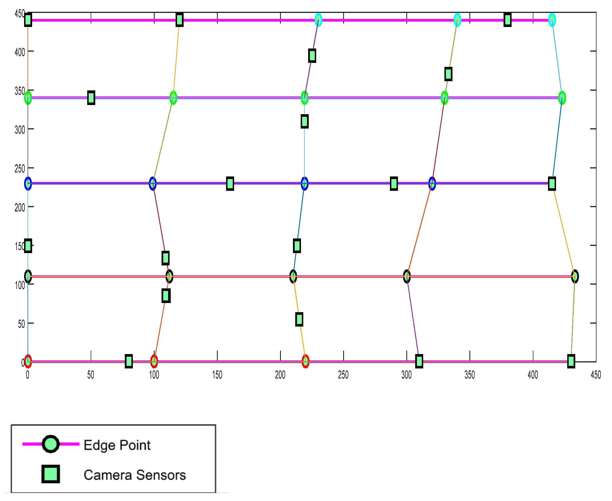
4.1. Simulation Setup

The proposed approach was evaluated using the MATLAB simulation tool. For the purpose of comparison with Ref. [20], the same testing environment, which is a square topology, was used. The size of the environment is 450 m × 450 m. A set of camera sensors were deployed randomly in the edges of the testing area. A picture of the simulated environment is shown in Figure 5. The figure could represent a building composed of five floors where each floor has five intersections or an area composed of [5 × 5] streets with an edge length of [80, 120]. Each camera sensor has an initial energy of 200 J. The parameters that were used in the simulation are shown in

Table 5. Simulation parameters.

Parameters	Values
Area Size (m2)	450 × 450
Camera Number	20, 30, 40
Round	50
Moving Distance of Target (m)	1000–4000
Visual sight of a Camera (m)	10–40
Initial Energy	200 J
Switch Energy	0.026 J
Consumed Energy	0.6 J
Sensing Energy	0.028 J

.

The performance analysis of the proposed approach is performed using the following metrics:

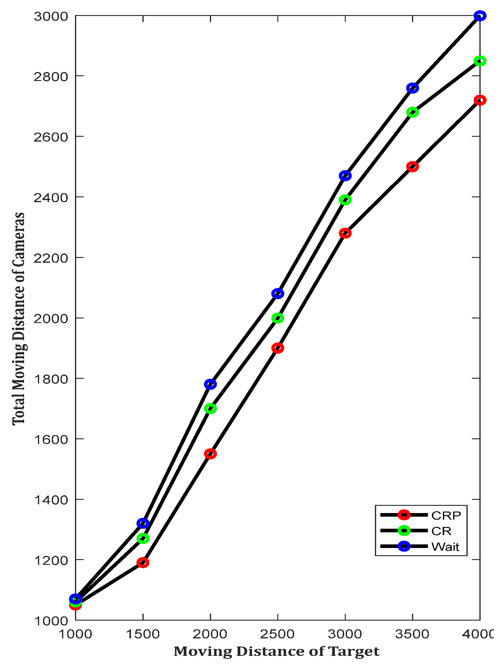
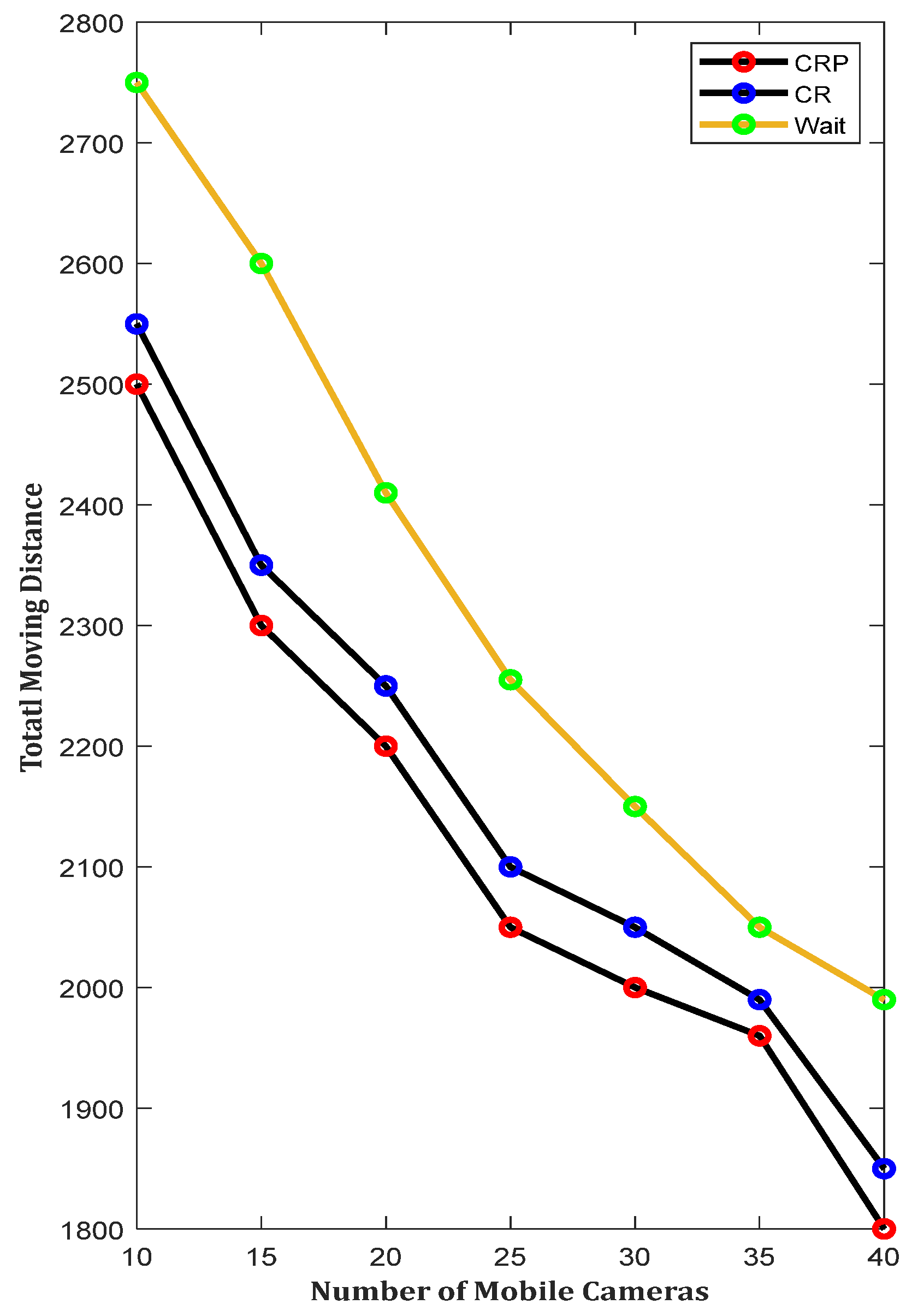
• The total moving distance of the cameras;
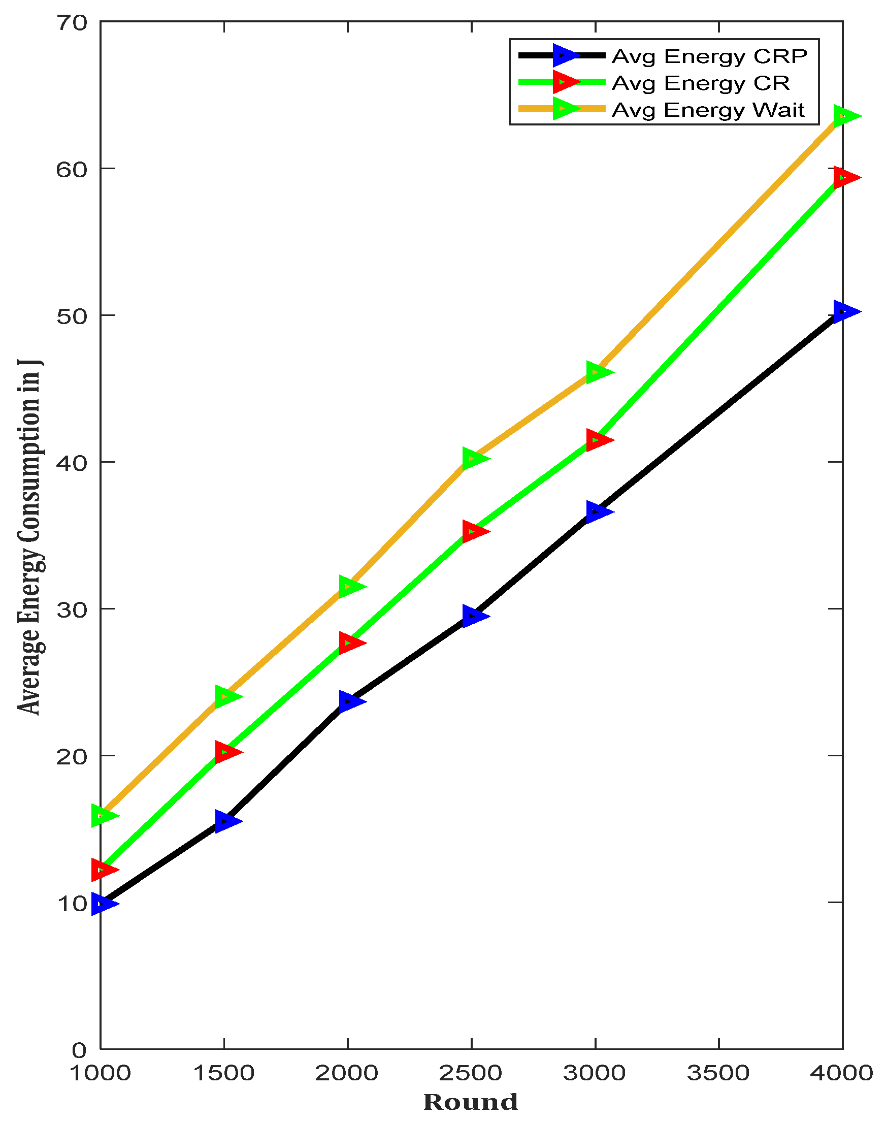
• The total energy consumed by the cameras;
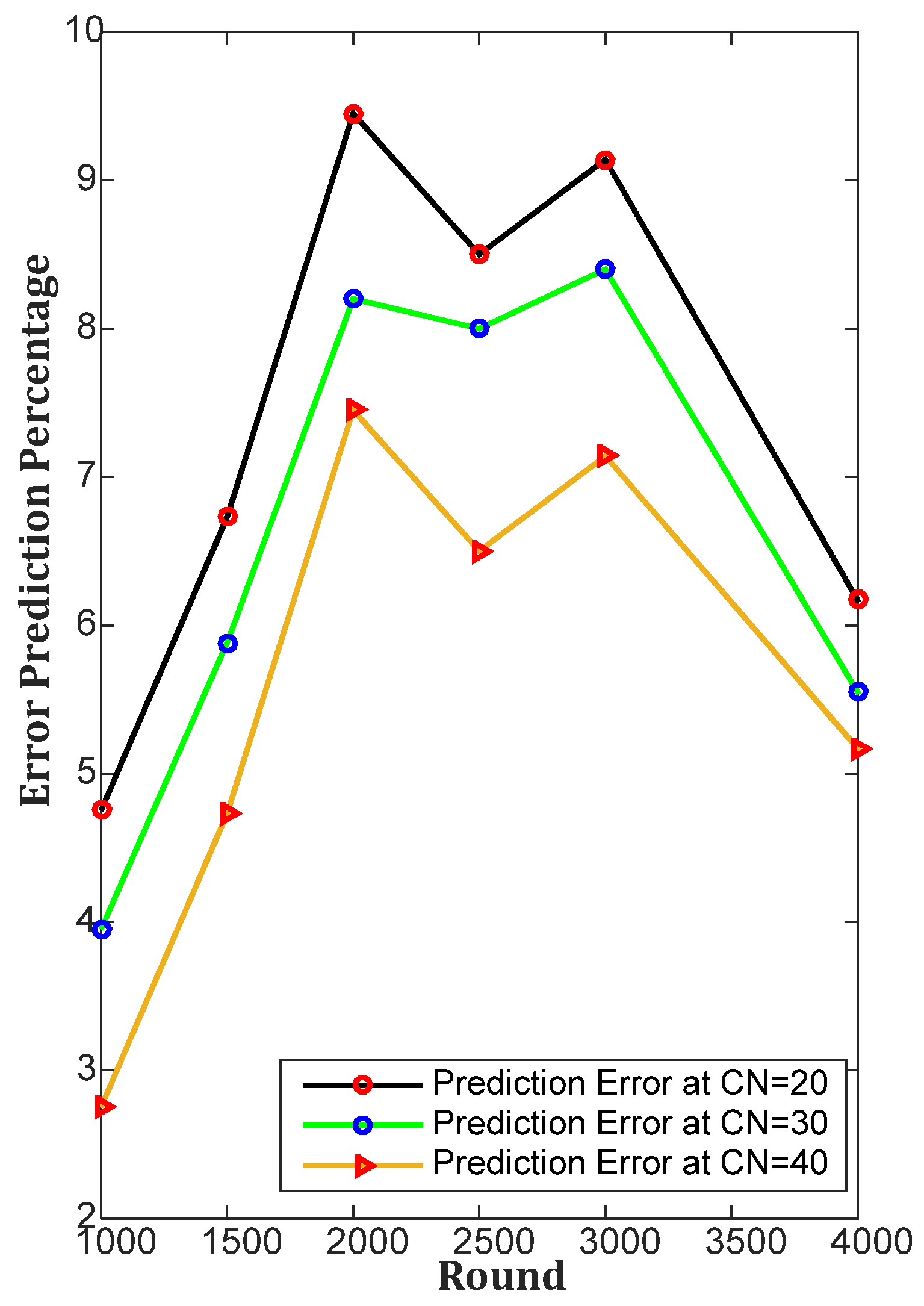
• The prediction error;
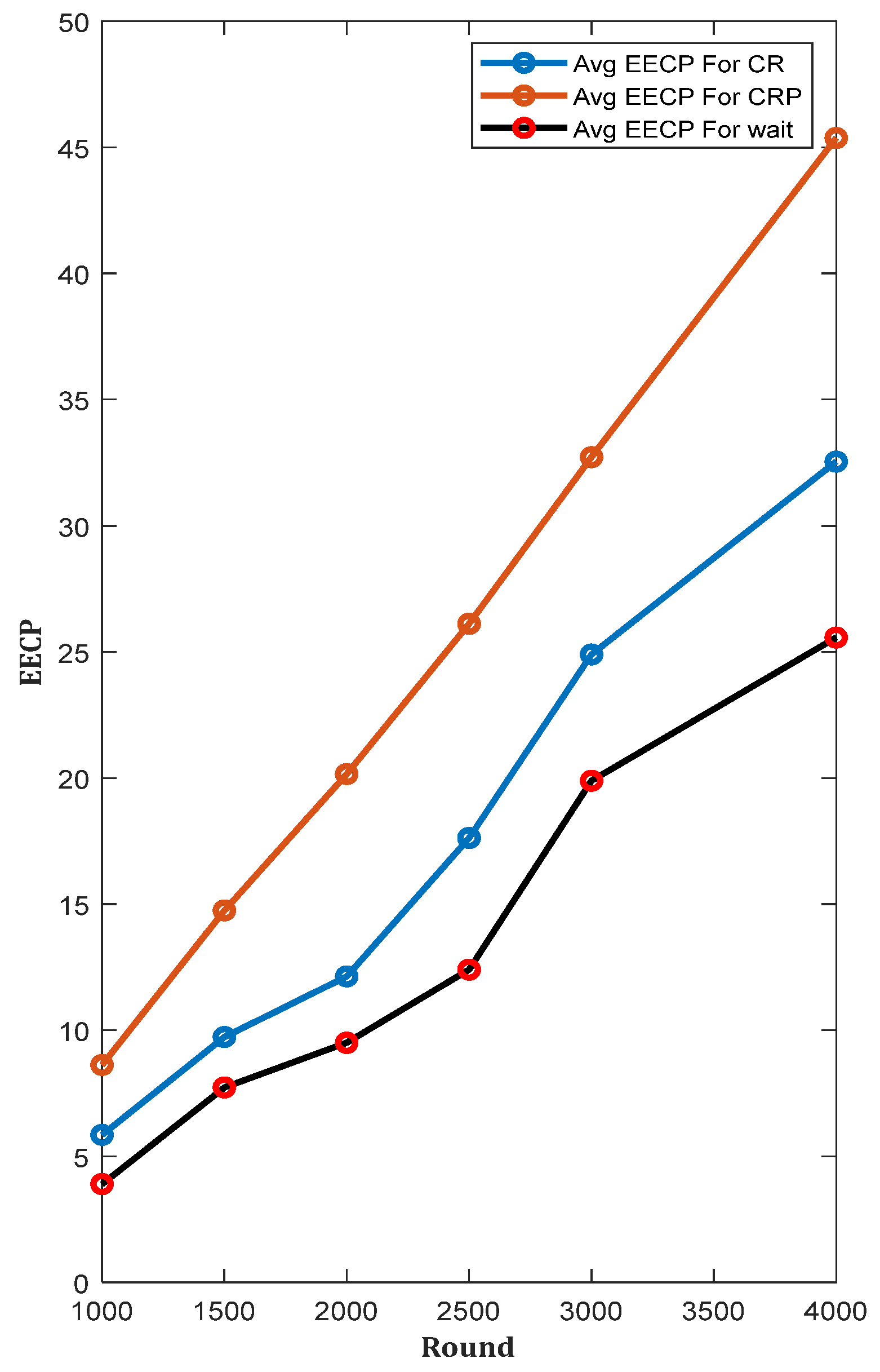
• The effective energy cost percentage (EECP), which is calculated as:

$$\mathrm{EECP} =\frac{E_{detected nodes}}{E_{active nodes} }$$

(10)

where E_{detected nodes} is the energy consumed by the nodes that actually detect the target, and E_{active nodes} is the energy consumed by all the nodes that were set in the active state.

4.2. Simulation Results

In this section, we discuss the simulation results that were produced by conducting several experiments. We compare the proposed enhanced cooperative relay tracking with prediction (CRP) algorithm with the camera relay (CR) algorithm proposed in [20] and the Wait algorithm, which is an approach of scheduling the cameras such that they will wait until the relay occurs.

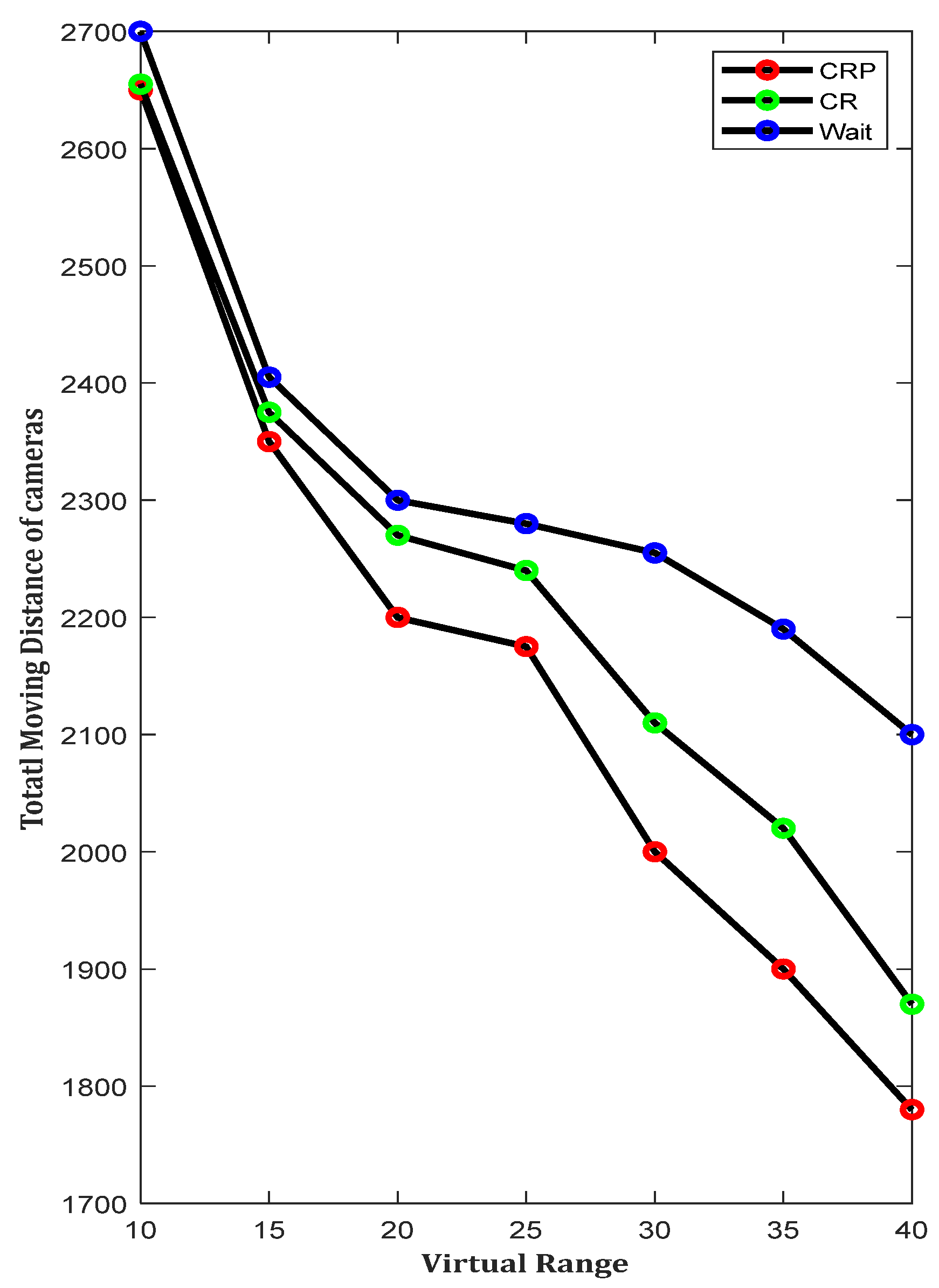
4.2.1. The Total Moving Distance of the Cameras

Figure 6 shows the total moving distance of cameras vs. virtual range. When the number of cameras is 20, the visual range increases from 10 m to 40 m, and the target’s total path is 3000 m. As shown in the figure, the overall distance decreases as the visual range increases. This can be justified as when the visual range is high, the distance will be reduced since increasing the value of the visual range will increase the probability of finding the shortest path for each camera. This will result in the overall moving distance of all cameras decreasing. Moreover, the proposed CRP protocol represents a significant improvement compared with the Wait and CR protocols. For example, when the virtual range is 40 m, the moving distance of cameras is 1780 m in the case of the CRP protocol, 1782 m in the case of the CR protocol, and 2100 m in the case of the Wait protocol. This means that the CRP protocol reduces the total moving distance by 5% compared with the CR protocol and by 15.2% compared with the Wait protocol.

Figure 7 shows the relationship between the moving distance of the target when it increases from 1000 m to 4000 m and the total moving distance of 20 cameras when the visual range is set to 25 m. It shows that the total moving distance of the cameras increases as the distance of the target increases. This is an intuitive conclusion: as the target moves into the area, more cameras will be activated in order to keep it under surveillance. Therefore, the total moving distance of cameras will increase as well. However, as shown in Figure 7, our proposed CRP tracking approach is more efficient than the CR and Wait algorithms due to its ability to schedule the cameras in advance. For example, when the moving distance of the target was 4000 m, the CRP protocol recorded 2720 m, the CR protocol recorded 2850 m, and the Wait protocol recorded 2999 m. This means that the CRP protocol reduces the total moving distance by 4.6% compared with the CR protocol and by 9.2% compared with the Wait protocol.

Figure 8 presents the distance differentiation when the number of cameras is increased from 10 to 40 and the visual range is set to 25 m. For each number of used cameras, the target moves randomly for a distance of 3000 m. It can be noticed that as the number of cameras increases, the process of relaying information between them becomes more frequent and more efficient, which results in a smaller total moving distance for all the activated cameras. This can be justified by saying that increasing the number of cameras will increase the options for selecting the next camera for activation. Therefore, the relying probability will be high due to the large number of available deployed cameras. However, in the real-life scenario, the cost problem should be taken into consideration because whenever the number of total cameras increases, the cost will increase too, which will affect energy efficiency as well. Therefore, there should be a compromise between the number of used cameras and their cost and consumed energy such that the deployment of the cameras in the environment guarantees the coverage of all areas while taking the cost and energy issues into consideration.

4.2.2. The Total Energy Consumed by the Cameras

Figure 9 compares our CRP prediction approach in terms of energy consumption with the CR and Wait algorithms. In this experiment, the number of cameras is 20, the distance moved by the target is 3000 m, and the camera’s visual range is 25 m. As shown in the figure, the CRP approach gives better energy savings due to the active-sleep schedule and the advanced path prediction. As shown in the figure, at round 4000, the energy consumed by all camera sensors is 50.23 joules, while it is 59.37 joules in the CR approach and 63.59 joules in the case of the Wait protocol. This means the CRP approach achieves a 13.36% reduction in the consumed energy compared with the CR approach and a 21% reduction compared with the Wait approach.

While the camera sensors in the CR and Wait algorithms will be active all the time, the CRP algorithm will activate only the corresponding cameras that are responsible for detecting the object. Even though it will sometimes have to turn on all the sensors within a specific region, the overall energy consumption will be less than with typical relay tracking.

4.2.3. The Prediction Error

Figure 10 shows the prediction error percentage versus round for the proposed approach when the camera number is [20, 30, and 40]. The distance traveled by the target is 4000 m, and the camera’s visual range is 30 m. The prediction error percentage is calculated as the number of failed predictions over the total number of steps with respect to the number of cameras that were activated in each round. The figure shows the error percentage in each round, and these errors are independent of each other, which means that there is no relationship between the rounds and the values related to the movement log and the correctness of the prediction. However, it can be observed that the error percentage in every round is significantly smaller compared to the overall prediction moves, and its values are limited between 2.7% and 9.5%.

4.2.4. The Effective Energy Cost Percentage (EECP)

Figure 11 illustrates the values of the effective energy cost percentage. A high EECP value implies that the protocol uses the energy more efficiently for the actual detection of the target, which is the desired goal of a wireless sensor network. A low EECP value, on the other hand, would indicate that a smaller proportion of the energy consumed by the nodes is being used for the actual detection of the target, which would be less efficient and may not achieve the desired goal of the network.

Compared to the CR and Wait algorithm, the figure shows that our CRP approach has a higher average effective energy cost due to its ability to schedule the camera sensors to be active and sleep efficiently, while in the CR and Wait algorithm every sensor will be active all the time.

5. Conclusions

Target tracking using camera sensor networks has received wide attention in recent years. In this paper, we propose an approach called CRP that utilizes the mobility of camera sensors in order to enhance the cooperative operation between camera sensors by applying a pattern recognition algorithm based on the past records of the targets. The CRP approach predicts the future route of the moving object and then constructs a movement schedule for the camera sensors to determine which camera should move and stay active and which camera should take over the monitoring operation. Compared with the Wait approach and the CR approach that uses cooperation relaying without prediction, simulation results have shown that the proposed approach is more efficient in terms of reducing the total distance of the mobile cameras that are activated to track the object and in terms of reducing the energy consumed by camera sensors. For example, the reduced total distance of the camera sensors reaches 5% compared with the CR protocol and up to 15.2% compared with the Wait protocol. On the other hand, in terms of the consumed energy, the CRP approach achieves a 13.36% reduction in the consumed energy compared with the CR approach and a 21% reduction compared with the Wait approach. Furthermore, simulation results showed that the prediction error percentage is significantly small compared to the overall prediction moves.

The proposed approach is designed and limited for single target movement. As future work, we intend to study and propose algorithms for multiple target movements using a pattern recognition model to find the shortest distance between camera movements and achieve the energy-saving objective.

References

1. Floris, A.; Porcu, S.; Girau, R.; Atzori, L. An IoT-Based Smart Building Solution for Indoor Environment Management and Occupants Prediction. Energies 2021, 14, 2959. [Google Scholar] [CrossRef]
2. Tekler, Z.D.; Low, R.; Yuen, C.; Blessing, L. Plug-Mate: An IoT-based occupancy-driven plug load management system in smart buildings. Build. Environ. 2022, 223, 109472. [Google Scholar] [CrossRef]
3. Zhuang, D.; Gan, V.J.; Tekler, Z.D.; Chong, A.; Tian, S.; Shi, X. Data-driven predictive control for smart HVAC system in IoT-integrated buildings with time-series forecasting and reinforcement learning. Appl. Energy 2023, 338, 120936. [Google Scholar] [CrossRef]
4. Yang, C.; Wang, W.; Li, F.; Yang, D. A Sustainable, Interactive Elderly Healthcare System for Nursing Homes: An Interdisciplinary Design. Sustainability 2022, 14, 4204. [Google Scholar] [CrossRef]
5. Cavur, M.; Demir, E. RSSI-based hybrid algorithm for real-time tracking in underground mining by using RFID technology. Phys. Commun. 2022, 55, 101863. [Google Scholar] [CrossRef]
6. Kumar, T.; Srinivasan, R.; Mani, M. An Emergy-based Approach to Evaluate the Effectiveness of Integrating IoT-based Sensing Systems into Smart Buildings. Sustain. Energy Technol. Assess. 2022, 52, 102225. [Google Scholar] [CrossRef]
7. Rizk, H.; Torki, M.; Youssef, M. CellinDeep: Robust and accurate cellular-based indoor localization via deep learning. IEEE Sens. J. 2018, 19, 2305–2312. [Google Scholar] [CrossRef]
8. Hernández, N.; Parra, I.; Corrales, H.; Izquierdo, R.; Ballardini, A.L.; Salinas, C.; García, I. WiFiNet: WiFi-based indoor localisation using CNNs. Expert Syst. Appl. 2021, 177, 114906. [Google Scholar] [CrossRef]
9. Tekler, Z.D.; Low, R.; Gunay, B.; Andersen, R.K.; Blessing, L. A scalable Bluetooth Low Energy approach to identify occupancy patterns and profiles in office spaces. Build. Environ. 2020, 171, 106681. [Google Scholar] [CrossRef]
10. Tekler, Z.D.; Chong, A. Occupancy prediction using deep learning approaches across multiple space types: A minimum sensing strategy. Build. Environ. 2022, 226, 109689. [Google Scholar] [CrossRef]
11. Jang, J.; Seon, M.; Choi, J. Lightweight Indoor Multi-Object Tracking in Overlapping FOV Multi-Camera Environments. Sensors 2022, 22, 5267. [Google Scholar] [CrossRef] [PubMed]
12. Liu, Q.; Wang, G.; Li, F.; Yang, S.; Wu, J. Preserving privacy with probabilistic indistinguishability in weighted social networks. IEEE Trans. Parallel Distrib. Syst. 2016, 28, 1417–1429. [Google Scholar] [CrossRef]
13. Pasqualetti, F.; Zanella, F.; Peters, J.R.; Spindler, M.; Carli, R.; Bullo, F. Camera network coordination for intruder detection. IEEE Trans. Control Syst. Technol. 2013, 22, 1669–1683. [Google Scholar] [CrossRef] [Green Version]
14. Alam Bhuiyan, Z.; Wang, G.; Wu, J.; Cao, J.; Liu, X.; Wang, T. Dependable structural health monitoring using wireless sensor networks. IEEE Trans. Dependable Secur. Comput. 2015, 14, 363–376. [Google Scholar] [CrossRef]
15. Morbidi, F.; Mariottini, G.L. Active target tracking and cooperative localization for teams of aerial vehicles. IEEE Trans. Control Syst. Technol. 2012, 21, 1694–1707. [Google Scholar] [CrossRef]
16. Liao, Z.; Wang, J.; Zhang, S.; Cao, J.; Min, G. Minimizing movement for target coverage and network connectivity in mobile sensor networks. IEEE Trans. Parallel Distrib. Syst. 2014, 26, 1971–1983. [Google Scholar] [CrossRef]
17. Tan, R.; Xing, G.; Wang, J.; So, H.C. Exploiting reactive mobility for collaborative target detection in wireless sensor networks. IEEE Trans. Mob. Comput. 2009, 9, 317–332. [Google Scholar] [CrossRef]
18. Wang, G.; Alam Bhuiyan, Z.; Cao, J.; Wu, J. Detecting movements of a target using face tracking in wireless sensor networks. IEEE Trans. Parallel Distrib. Syst. 2013, 25, 939–949. [Google Scholar] [CrossRef] [Green Version]
19. Yu, Q.; Medioni, G.; Cohen, I. Multiple target tracking using spatio-temporal markov chain monte carlo data association. In Proceedings of the 2007 IEEE Conference on Computer Vision and Pattern Recognition, Minneapolis, MN, USA, 17–22 June 2007; pp. 1–8. [Google Scholar] [CrossRef]
20. Wang, T.; Zeng, J.; Alam Bhuiyan, Z.; Chen, Y.; Cai, Y.; Tian, H.; Xie, M. Energy-efficient relay tracking with multiple mobile camera sensors. Comput. Netw. 2018, 133, 130–140. [Google Scholar] [CrossRef]
21. Gao, X.; Yang, R.; Wu, F.; Chen, G.; Zhou, J. Optimization of full-view barrier coverage with rotatable camera sensors. In Proceedings of the 2017 IEEE 37th International Conference on Distributed Computing Systems (ICDCS), Atlanta, GA, USA, 5–8 June 2017; pp. 870–879. [Google Scholar] [CrossRef]
22. Reddy, V.P.; Fathima, A.A. Object Tracking Based on Position Vectors and Pattern Matching. In Computational Signal Processing and Analysis; Springer: Singapore, 2018; pp. 407–416. [Google Scholar] [CrossRef]
23. Zhang, X.; Wang, X.; Gu, C. Online multi-object tracking with pedestrian re-identification and occlusion processing. Vis. Comput. 2020, 37, 1089–1099. [Google Scholar] [CrossRef]
24. Tang, Z.; Hwang, J.-N. Moana: An online learned adaptive appearance model for robust multiple object tracking in 3d. IEEE Access 2019, 7, 31934–31945. [Google Scholar] [CrossRef]
25. Wang, T.; Jia, W.; Wang, G.; Guo, M.; Li, J. Hole Avoiding in Advance Routing with Hole Recovery Mechanism in Wireless Sensor Networks. Adhoc Sens. Wirel. Netw. 2012, 16, 191–213. [Google Scholar]
26. Yang, J.; Ge, H.; Yang, J.; Tong, Y.; Su, S. Online multi-object tracking using multi-function integration and tracking simulation training. Appl. Intell. 2021, 52, 1268–1288. [Google Scholar] [CrossRef]
27. Hu, Y.; Wang, X.; Gan, X. Critical sensing range for mobile heterogeneous camera sensor networks. In Proceedings of the IEEE INFOCOM 2014-IEEE Conference on Computer Communications, Toronto, ON, Canada, 27 April–2 May 2014; pp. 970–978. [Google Scholar] [CrossRef]
28. Wang, Y.; Song, Y.; Gao, H.; Lewis, F.L. Distributed fault-tolerant control of virtually and physically interconnected systems with application to high-speed trains under traction/braking failures. IEEE Trans. Intell. Transp. Syst. 2015, 17, 535–545. [Google Scholar] [CrossRef]
29. Qi, Y.; Cheng, P.; Bai, J.; Chen, J.; Guenard, A.; Song, Y.-Q.; Shi, Z. Energy-efficient target tracking by mobile sensors with limited sensing range. IEEE Trans. Ind. Electron. 2016, 63, 6949–6961. [Google Scholar] [CrossRef]
30. Tsai, R. A versatile camera calibration technique for high-accuracy 3D machine vision metrology using off-the-shelf TV cameras and lenses. IEEE J. Robot. Autom. 1987, 3, 323–344. [Google Scholar] [CrossRef] [Green Version]
31. Zhang, Z. A flexible new technique for camera calibration. IEEE Trans. Pattern Anal. Mach. Intell. 2000, 22, 1330–1334. [Google Scholar] [CrossRef] [Green Version]
32. Liu, X.; Kulkarni, P.; Shenoy, P.; Ganesan, D. Snapshot: A self-calibration protocol for camera sensor networks. In Proceedings of the 2006 3rd International Conference on Broadband Communications, Networks and Systems, San Jose, CA, USA, 1–5 October 2006; pp. 1–10. [Google Scholar] [CrossRef] [Green Version]
33. Funiak, S.; Guestrin, C.; Paskin, M.; Sukthankar, R. Distributed localization of networked cameras. In Proceedings of the 5th International Conference on Information Processing in Sensor Networks, Nashville, TN, USA, 19–21 April 2006; pp. 34–42. [Google Scholar]
34. Chu, M.; Reich, J.; Zhao, F. Distributed attention in large scale video sensor networks. IEEE Intell. Distrib. Surveilliance Syst. 2004, 61–65. [Google Scholar] [CrossRef]
35. Liao, W.-H.; Chang, K.-C.; Kedia, S.P. An object tracking scheme for wireless sensor networks using data mining mechanism. In Proceedings of the 2012 IEEE Network Operations and Management Symposium, Maui, HI, USA, 16–20 April 2012; pp. 526–529. [Google Scholar] [CrossRef]
Figure 1. An example of cooperative relay tracking and prediction of targets is in the mall.
Jsan 12 00035 g001
Figure 2. An example of CSN environment and its graph model.
Jsan 12 00035 g002
Figure 3. Steps of the pattern recognition algorithm.
Jsan 12 00035 g003
Figure 4. An illustration of how pattern recognition algorithm works.
Jsan 12 00035 g004
Figure 5. An example of a simulation environment.
Jsan 12 00035 g005
Figure 6. Total moving distance of cameras vs. virtual range.
Jsan 12 00035 g006
Figure 7. Total moving distance of cameras vs. moving distance of target.
Jsan 12 00035 g007
Figure 8. Total moving distance vs. number of mobile cameras.
Jsan 12 00035 g008
Figure 9. Energy consumption of nodes vs. round.
Jsan 12 00035 g009
Figure 10. Prediction error vs. round.
Jsan 12 00035 g010
Figure 11. EECP vs. round.
Jsan 12 00035 g011