1. Introduction
Multiple sensor nodes make up a wireless sensor network (WSN), where these nodes can sense, measure, gather, and transmit information from the environment via radio. In a wide range of applications, such as healthcare, industrial control, public security, commercial, military, and environmental monitoring, WSNs are widely used [
1,
2,
3]. A WSN has limited storage, battery, and processing capacity, which affects the network lifetime, quality of service, and cost [
4,
5]. Furthermore, data collection and transmission in WSNs may be affected by attacks or interference in harsh environments. Therefore, a WSN’s reliability is an important issue, to be sure that the WSN works properly. It is essential to calculate WSN reliability, to minimize the cost, minimize the node power consumption, and maximize the network lifetime, as unreliable WSNs may fail to accomplish the tasks, resulting in inefficient use of sensor resources [
6]. The reliability of the WSN can be evaluated using various methods such as Markov chain theory, universal generating function (UGF), a Monte Carlo (MC) simulation approach, a reliability block diagram (RBD), fault tree (FT) [
7], and a signal strength and trust model [
8].
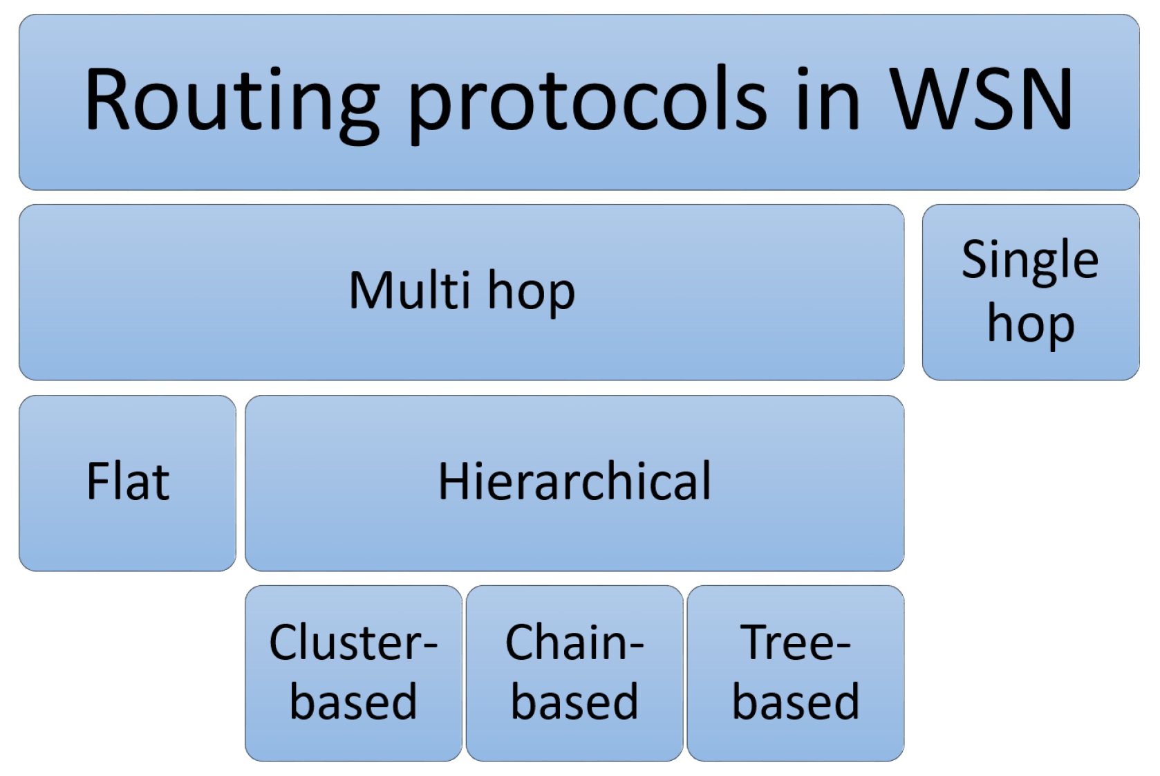
The routing issue in transferring data from the source node to the target node is one of the most significant challenges facing WSNs. Existing routing protocols can be classified into single-hop and multi-hop, where in single-hop, the data is directly sent from the node to the base station (BS), while the data is sent to the BS through several nodes in multi-hop [
5]. Multi-hop routing protocols fall into two main categories based on the network structure: hierarchical and flat [
9,
10,
11]. In the flat routing protocol, all nodes perform the same task and function. Whereas in hierarchical routing protocols, different tasks and functions are assigned to the nodes [
10,
12,
13,
14]. The three main types of the flat routing protocol are: proactive (table-driven), reactive (source-initiated), and hybrid [
10]. RPL, Hydro, CPT, and Zigbee are the most popular proactive routing protocols [
15,
16]. LOAD, LOADng, AODVbis, and Tiny AODV are some examples of reactive routing protocols [
15,
16,
17]. Moreover, zone routing is an example of hybrid routing protocols.
Figure 1 illustrates the three main types of hierarchical routing protocols: cluster-based, tree-based, and chain-based [
2,
5,
9,
13,
18].
In cluster-based routing [
19,
20,
21,
22], each cluster has at most one cluster head (CH) that manages the cluster, while other nodes are called cluster members (CMs), as illustrated in
Figure 2, where the CMs send the collected data to the CH and do not directly communicate with the BS. In the WSN, the BS serves as both the central data-collecting node and the common destination for data gathered from the nodes. There are usually no power restrictions on the BS, which acts as a bridge between WSN and the end user (via communication). The most popular cluster-based routing protocol is the low-energy adaptive clustering hierarchy (LEACH) [
13].
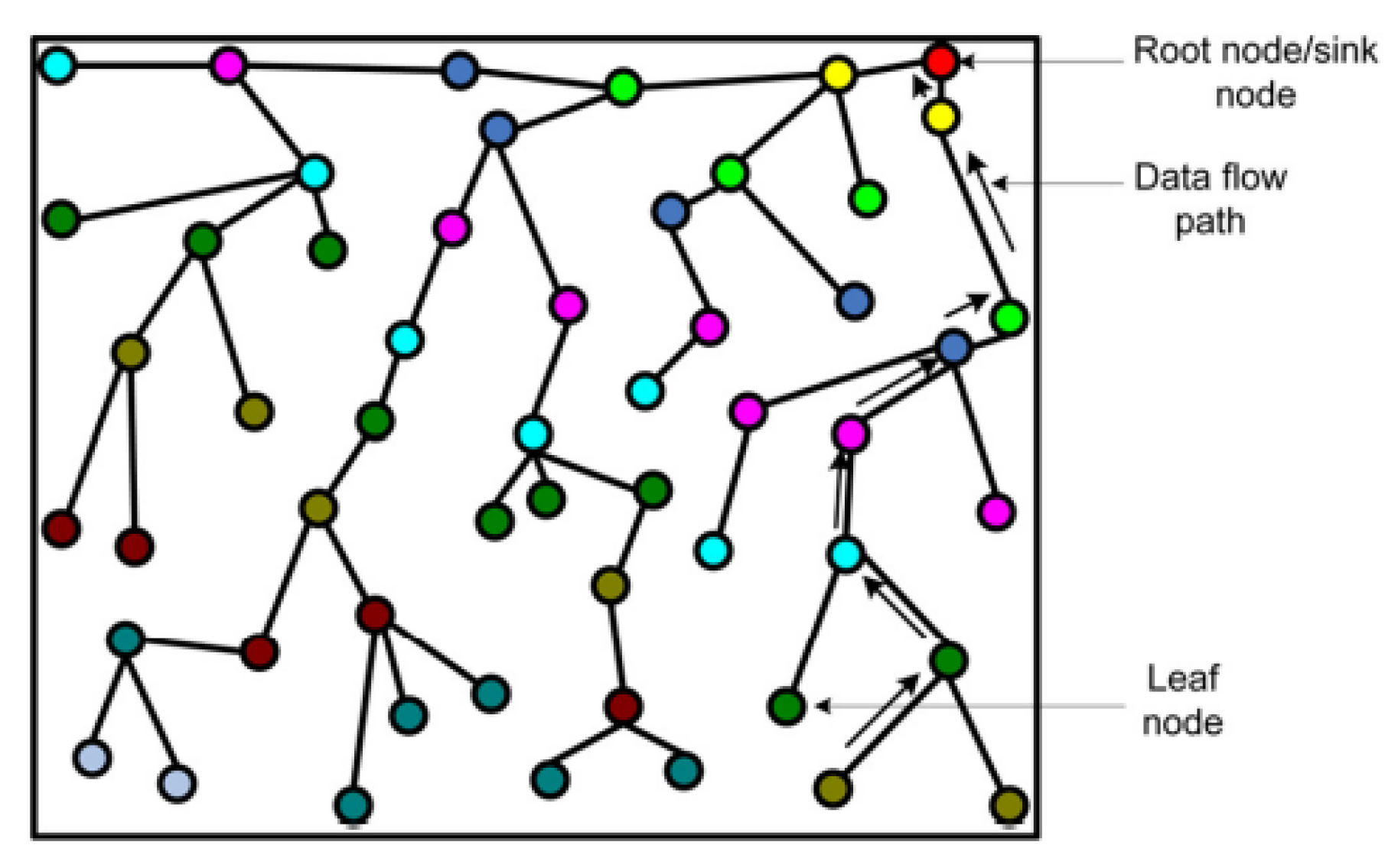
As shown in
Figure 3, the tree-based topology deploys nodes in a logical tree configuration, with all sensor data being transferred from leaf nodes (children) to their respective parents [
12,
18].
An appropriate neighbor node is selected as the parent node for every node in a tree-based approach. A routing tree is constructed with a sink node that acts as a root node, and all nodes are connected to the root through the most energy-saving path [
23]. The sensor node’s data is transmitted along the tree towards the root node (sink) and is fused between nodes. There are different tree-based routing protocols such as energy-aware data aggregation tree (EADAT), balanced aggregation tree routing (BATR), power-efficient data gathering and aggregation protocol (PEDAP), and enhanced tree routing (ETR) [
18].
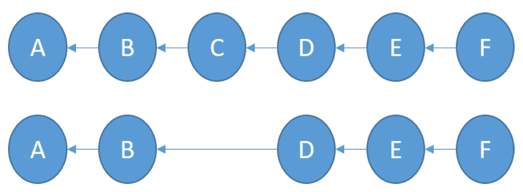
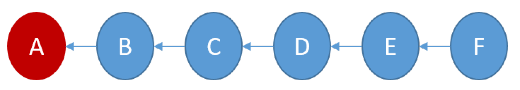
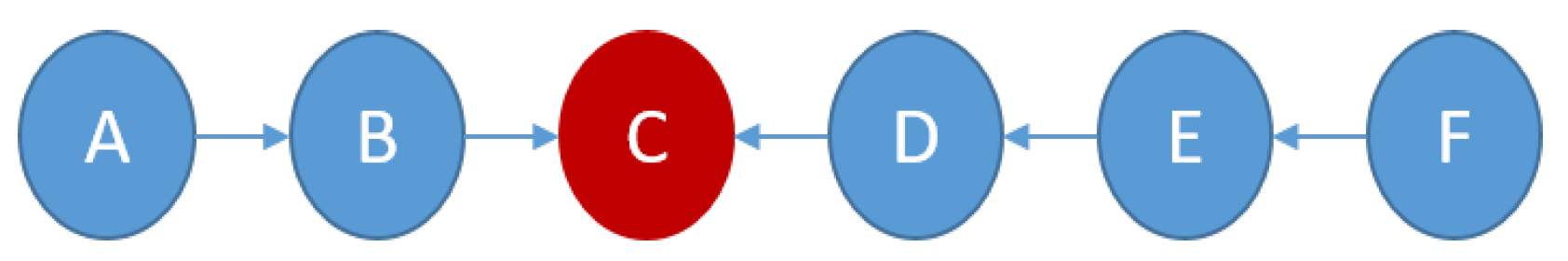
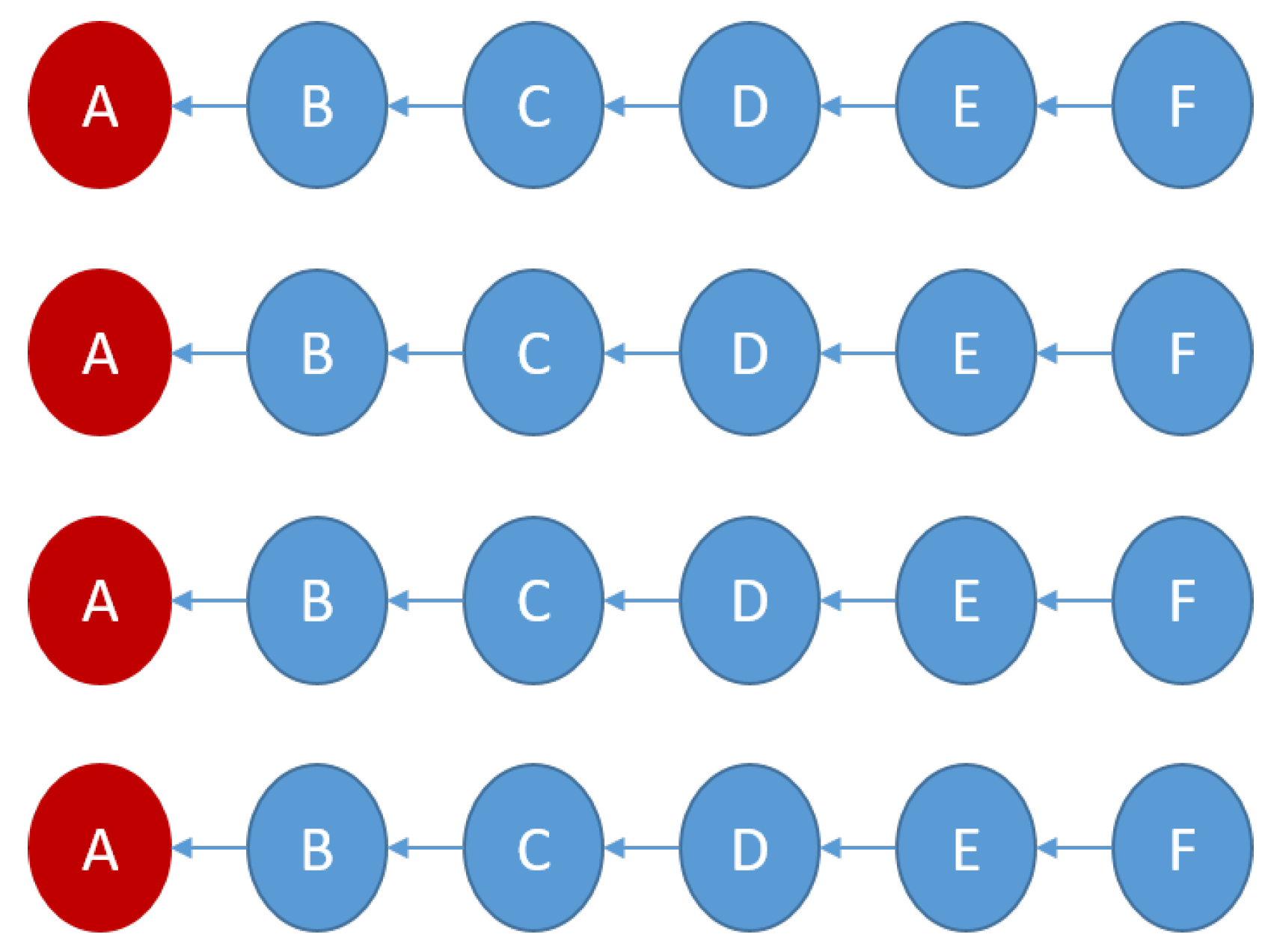
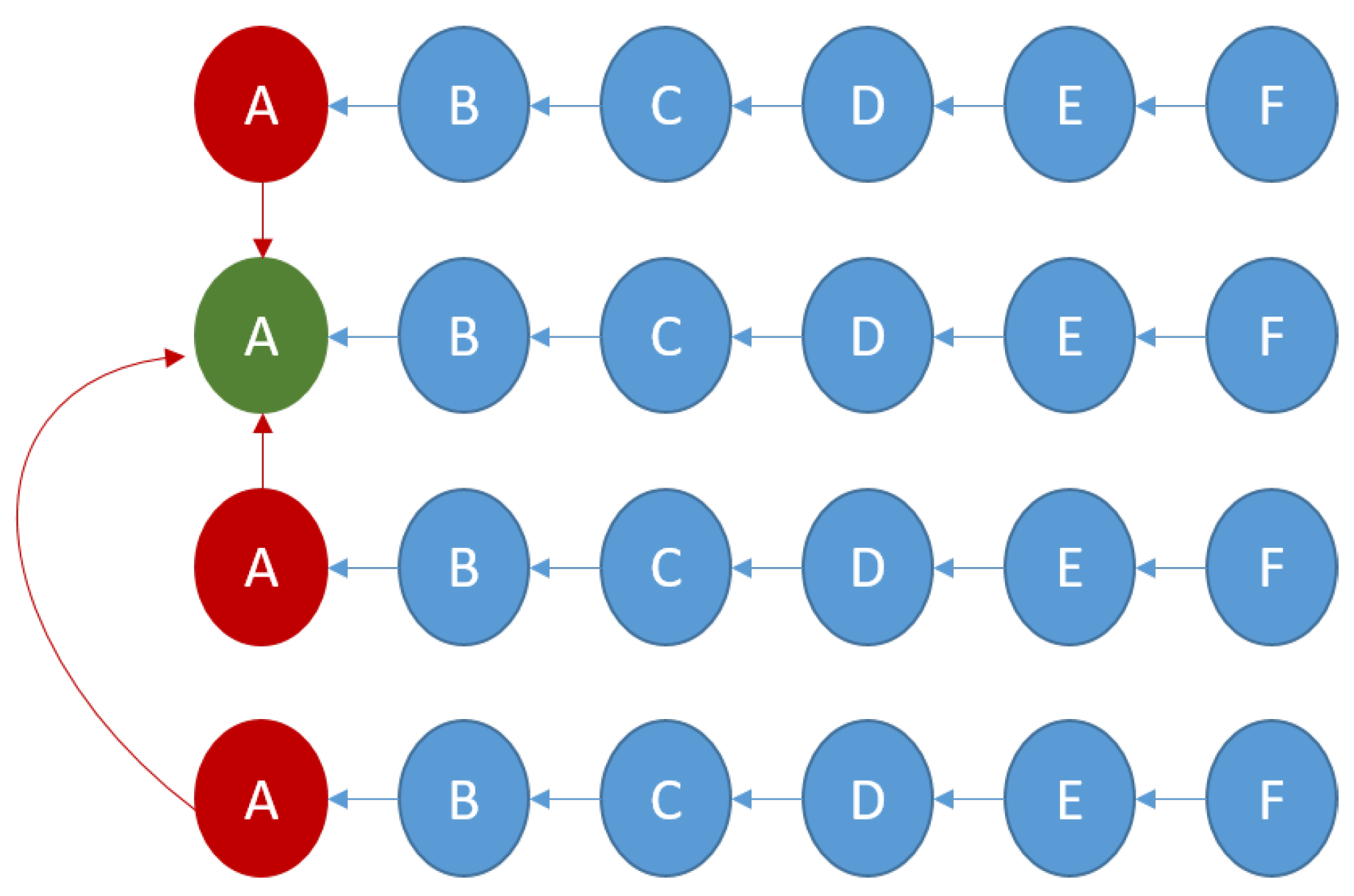
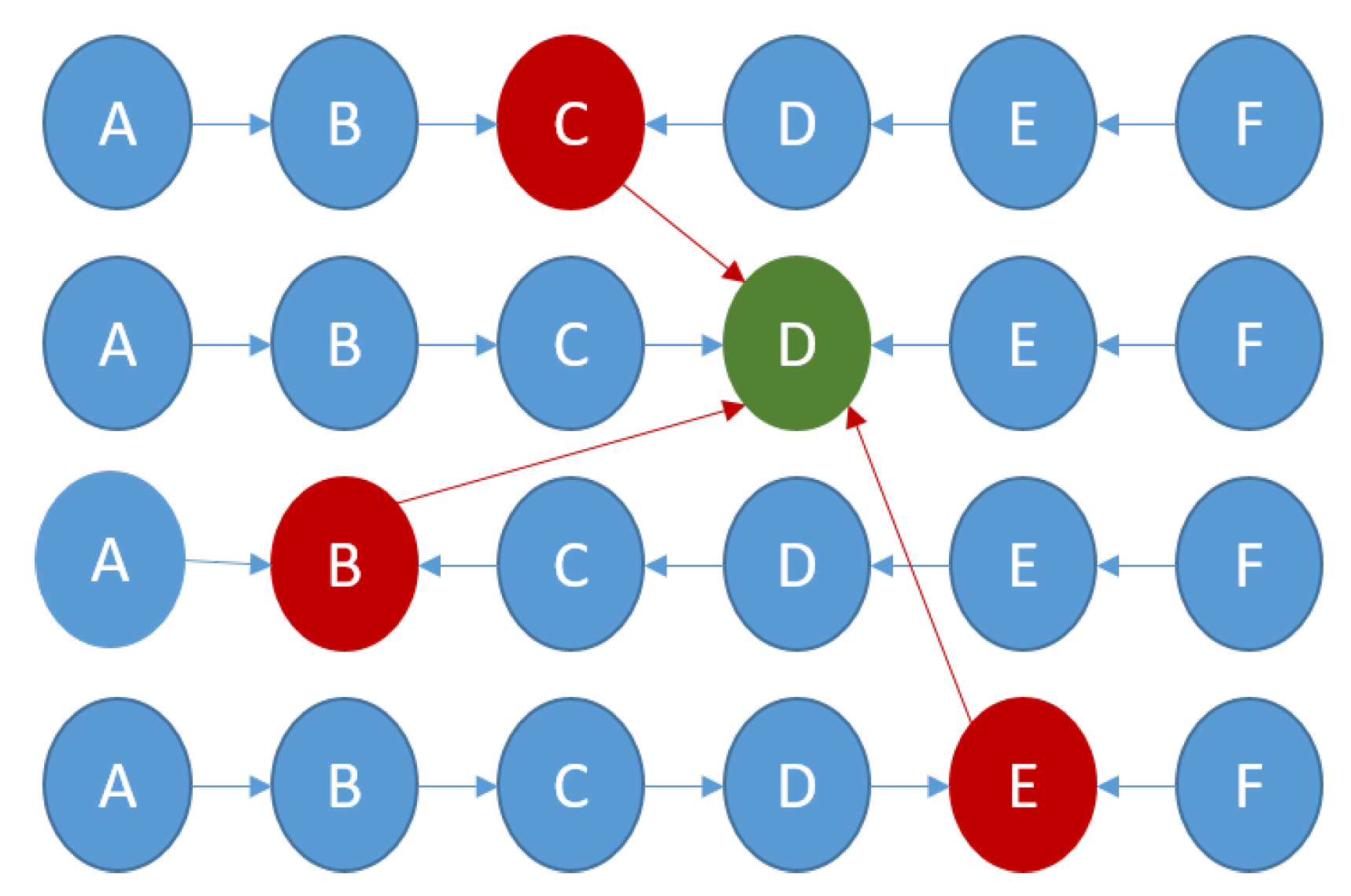
On the other hand, chain-based topology arranges nodes to form and construct chains, where each chain has a chain leader and sensor nodes, as shown in
Figure 4 [
9]. In WSN, a chain can be built either by the nodes themselves, using a greedy strategy, or by the BS, which will calculate and broadcast the chain to all nodes. Single chains or multi-chains can be constructed in chain-based routing. Chain-based routing is simpler to configure and maintain than cluster-based routing [
13,
18]. Furthermore, local communication conserves energy compared to cluster-based routing, since nodes only transmit data to nearby nodes (i.e., their next nearest neighbor nodes) [
12,
18,
24]. There are various protocols and algorithms that can be implemented based on chain routing, such as power efficient gathering in sensor information systems (PEGASIS), concentric clustering scheme (CCS), balanced chain-based routing protocol (BCBRP), and rotation PEGASIS-based (RPB) [
2,
13,
18]. However, the most popular protocol is PEGASIS, where a chain is constructed from the farthest node from the BS, followed by the closest not-connected neighbor node, and so on [
13]. The chain head is responsible for data aggregation and data processing. Therefore, a new chain head can be selected randomly in the event that the current chain head fails.
In this paper, we focus on hierarchical routing protocols that are categorized according to the network structure, particularly chain-based routing protocols. There are a number of applications that benefit from chain-based topology, including monitoring coal mine gas, periodic monitoring of building conditions, wind power, parking management systems, IoT-WSN-based smart agricultural environments, and underwater smart things. Furthermore, a chain-based topology can be applied as part of a fog-supported WSN, along with other topologies [
9,
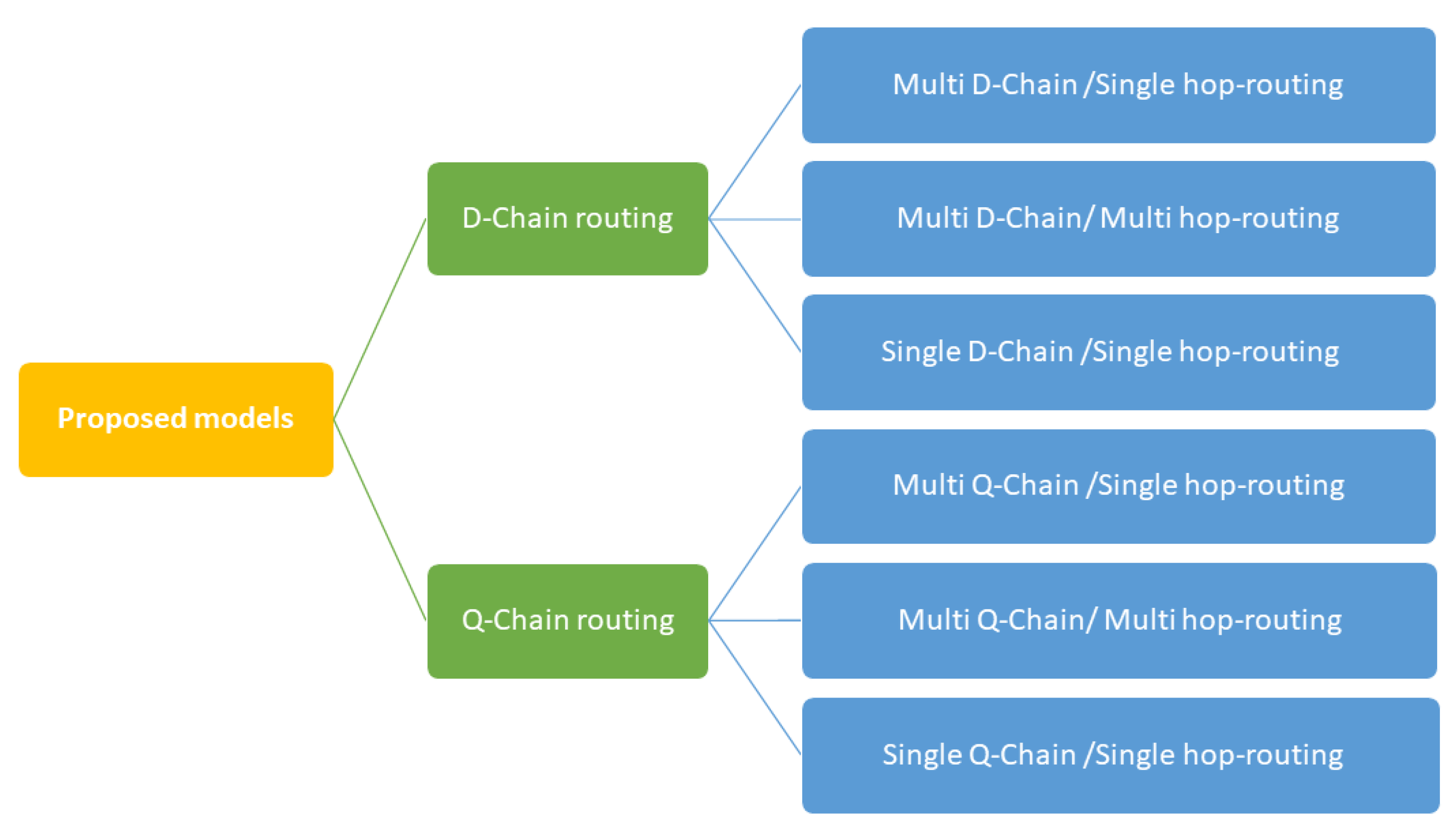
25]. This work proposes various chain configurations and evaluates the system reliability of different proposed chain-based routing models, based on the proposed RBD in WSN. The power consumption for each node is the main factor that is considered to evaluate the system’s reliability. The main contributions of this work are summarized below:
Various chain-based routing models are considered and discussed.
Chain head selection approaches that are based on weight Q, or distance D, are investigated and evaluated.
We propose a new RBD-based methodology, to evaluate the reliability of different chain-based routing models in cases of fixed and dynamic chain head settings, where the node reliability is evaluated based on energy.
The work in this paper is presented as follows:
Section 2 presents the related work. The background of the reliability block diagram is illustrated in
Section 3. The proposed model is presented in
Section 4.
Section 5 discusses the experimental setup and results, and
Section 6 gives the conclusions of our proposed work.
2. Related Work
This section demonstrates the previous studies regarding evaluating the system reliability of WSNs. The different techniques for evaluating WSN reliability are discussed. Moreover, analyzing and calculating WSN reliability-based RBD is illustrated.
Studies, evaluations, and analyses of WSNs’ reliability have been previously carried out in several studies [
26,
27]. Evaluation of the reliability of a WSN can be conducted utilizing different techniques, of which the most well-known are a universal generating function [
28], a Markov model [
29], a fault tree [
30], and a Monte Carlo simulation [
31], where the authors utilized an ordered binary decision diagram (OBDD) beside a Monte Carlo simulation, to evaluate the WSN’s reliability. The authors of [
32] proposed a Monte Carlo Markov chain simulation method to evaluate the reliability, regarding data capacity and coverage area, of mobile WSNs with multi-state nodes, but the power consumption was not taken into account. A Markov model was proposed in [
33], to address the reliability of sensor nodes in a WSN-based monitoring strategy, but power consumption was not considered. A modified sum of disjoint products approach was proposed in [
34], for evaluating the reliability of WSN with multi-state nodes, where the reliability was evaluated based on the network’s dynamic state only. The reliability evaluation of WSNs and compromised node identification was described in [
8], where an enhanced way of evaluating reliable nodes was proposed to protect the entire WSN from compromised nodes. A new efficient algorithm-based OBDD was proposed in [
6], to evaluate WSN reliability, where the proposed approach executed the recursive construction of OBDD once. A new sum of disjoint products technique (SDP) was proposed in [
35] to generate disjoint products and calculate the network reliability. Moreover, probabilistic analysis was utilized to evaluate the network transmission reliability in [
36], where the required retransmission was decreased and the transmission reliability was improved.
The reliability block diagram paradigm (RBD), is one of the most useful techniques to calculate reliability [
37,
38]. The reliability was evaluated via RBD in the following studies: RBD was applied in [
37], to analyze the reliability of a mesh network that consisted of different tree and star networks and was classified as a series–parallel system. The authors of [
39] evaluated the reliability of star and cluster WSNs with dynamic dependent nodes based on dynamic RBD (DRBD), where it overcame the Markov model’s limitations because it considered nonlinear discharge processes. Furthermore, the author in [
40] calculated the reliability of star, cluster, and mesh WSNs, with sleep/wake-up interfering nodes-based DRBD and Petri nets, which overcame the Markov model’s limitations according to nonlinear processes. Since RBD overcomes the limits of the Markov model, RBD is utilized to evaluate WSNs’ reliability in [
5], considering the DIRECT, FLOODING, and LEACH routing algorithms and battery level. In [
41], the reliability of a mesh WSN was analyzed and evaluated, based on RBD and fault tree analysis. Moreover, the authors studied the effects of way redundancy and node arrangements on reliability. The authors in [
42] analyzed the reliability of WSN data transport protocols based on RBD and the higher-order logic theorem prover.
Reliability is an important factor to consider when evaluating the performance of WSNs since it can be evaluated according to network power, where a dead sensor node is unable to transmit data and affects the entire system. The reliability of different network topologies in WSN-based RBD has been evaluated in a range of studies, except for chain routing, which has not been examined in any studies. All published works have assumed the same concept of probability, where probability is 1 for a working node and 0 for a failure node. However, in our proposed RBD, the probability of each node is evaluated based on the ratio between the residual energy and the initial energy of the node. Moreover, all the previous research assumes that the system fails in series configuration if any node fails, while our proposed RBD continues the reliability evaluation until the chain head dies, in the case of a stationary chain head, or till the network dies, in the case of a dynamic chain head.
3. Reliability Block Diagram (RBD)
RBD is a technique for evaluating the reliability of a whole system. All the components of a system are represented graphically, and their reliability determines the overall system’s reliability. A block indicates whether a component is working or not, so the reliability depends on the configurations of the components [
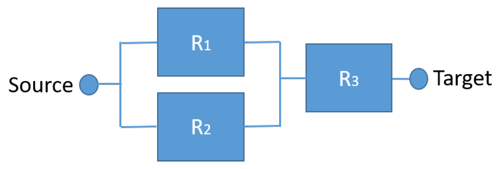
41]. A series configuration, a parallel configuration, and a combined (hybrid) configuration are the most commonly used configuration types, as shown in
Figure 5,
Figure 6 and
Figure 7, respectively [
5]. Whenever a component fails in a series configuration, the entire system fails. Thus, the least reliable component is the one that has the most impact on the overall reliability. Therefore, the reliability of a system in series is lower than the reliability of the least reliable component.
In a series system, reliability is defined as the product of the reliability of the components that make it up (series reliability = R1 × R2 × R3), where R1, R2, and R3 represent the working reliability of components 1, 2, and 3, respectively [
43]. For a parallel system to function properly, at least one unit must function.
In a parallel configuration, the system reliability is largely affected by the item characterized by the highest reliability trend, where the system reliability is derived from the complement of the product of the reliability of each component (parallel reliability = 1 − ((1 − R1) × (1 − R2) × (1 − R3))) [
43].
In a hybrid configuration, combining blocks creates other formats: series–parallel, parallel–series, bridge, and k-out-of-n. In order to solve the reliability problem, the parallel blocks must first be solved, and then the series blocks (hybrid reliability = R3 × (1 − ((1 − R1) × (1 − R2)))).


