Loitering Detection Using Spatial-Temporal Information for Intelligent Surveillance Systems on a Vision Sensor

Abstract

As one of the essential modules in intelligent surveillance systems, loitering detection plays an important role in reducing theft incidents by analyzing human behavior. This paper introduces a novel strategy for detecting the loitering activities of humans in the monitoring area for an intelligent surveillance system based on a vision sensor. The proposed approach combines spatial and temporal information in the feature extraction stage to decide whether the human movement can be regarded as loitering. This movement has been previously tracked using human detectors and particle filter tracking. The proposed method has been evaluated using our dataset consisting of 20 videos. The experimental results show that the proposed method could achieve a relatively good accuracy of 85% when utilizing the random forest classifier in the decision stage. Thus, it could be integrated as one of the modules in an intelligent surveillance system.

1. Introduction

The development of intelligent surveillance systems (ISS) has become significantly popular due to increasing demand for security and safety in public spaces [1,2]. The ISS configures a set of vision sensors, e.g., closed circuit television (CCTV), installed in different areas and a server/command center connected to a computer network. The ISS can analyze the image, audio, and video generated by the vision sensor to identify anomalous events with limited human intervention in the monitoring area using artificial intelligence technologies such as computer vision, pattern recognition, machine learning, etc. [2]. For example, the ISS might contain various modules that analyze a specific anomaly case.

As one of its applications, the ISS could be used to reduce crime rates, for example, in theft cases. In this case, the ISS should be able to prevent theft incidents. So, we need a module integrated with ISS to detect possible theft cases before the incident occurs.

One way to detect possible theft cases is to identify the suspicious behavior of human objects in the monitoring area, namely loitering. In loitering detection, the system must be able to detect the presence of human objects and track their movements. The movement of human objects involves the spatial domain associated with the position of the object in the monitoring area, as well as the temporal domain related to the duration of the event. However, only some previous papers have exploited these two pieces of information in detecting loitering. Therefore, we propose to use both pieces of information as part of the feature extraction stage.

Several previous studies related to loitering detection used two approaches. The first approach uses handcrafted features [3,4,5,6,7,8], while the second uses non-handcrafted features (deep learning) [9,10]. In the handcrafted feature approach, the steps can be divided into three parts: (1) the person-detection process, (2) the feature extraction used to distinguish normal videos and videos that contain people loitering based on the detected person’s movements, and (3) the video classification process. As for the non-handcrafted feature approach, the video input goes directly into a deep-learning architecture. The neural network layers in the deep-learning architecture function as a feature extractor and a classifier.

The features used to identify loitering can vary in the handcrafted feature approach. For example, the total time a person is in the area on the surveillance camera could be used as a feature. The system will detect loitering if the occurrence of a person exceeds the duration limit in the surveillance area. After the person detection and tracking stage, each duration in a particular area will be compared with the safe time limit of 10 s [3]. If people are in a specific area for over 10 s, then that person is identified as loitering. Patel et al. [4] used the same features, but only the time limit is adjusted adaptively based on the movement of the person in the frame.

Another feature that can be used is the angle formed by the movement of a person in a sequenced frame. Angle refers to the change in the center of gravity (CoG) of the detected person in a particular frame with the same person in the next frame [5]. The larger the angle formed, the greater the chance the person will do the lottery and vice versa.

Some researchers have tried combining time and changing angles as features [6,7]. The time limit was adjusted based on various video shooting areas (bus stops, shopping malls, railway stations, etc.) [6]. When a person passes the time threshold and has a significant angle change, that person is indicated to be loitering. If the values for these two features exceed the limit, the person in the frame loiters.

Apart from time and angle changes, optical flow is another handcrafted feature that can be used for loitering detection. Zhang et al. [8] associate the optical flows between multiple frames to capture short-term trajectories. The optical flow is then represented in a histogram. The next stage is clustering using k-nearest neighbor (KNN). The outlier data generated after the clustering process are assumed to be videos with a loitering person.

In the non-handcrafted feature approach, several deep-learning architectures can be used for loitering detection. The deep-learning architecture used is 2-Stream 3D-Convolutional Neural Network (3D-CNN) [9]. One branch uses input RGB frames, while the other uses optical flow frames. Asad et al. [10], used the deep-learning architecture in the form of a 3D convolutional autoencoder (3D-CAE). First, the spatiotemporal features of the last layer output of the 3D max polling are clustered using k-means. Then, the clusters are separated using Support Vector Machine (SVM) to distinguish between normal videos and videos with a loitering person.

We aim to integrate the loitering-detection module into a CCTV-based intelligent surveillance system (ISS). In the ISS, the speed of the process is crucial in responding quickly to detected abnormal events to prevent criminal activities as early as possible. Because of this requirement, the integrated module should be executed in real-time but still maintain performance. Therefore, this paper proposed a loitering-detection method based on spatial and temporal information and machine learning to achieve real-time processing and high accuracy in performance. Overall, the main contributions of the work are summarized as follows:

• Proposing a novel feature extraction based on spatial and temporal information for loitering detection.
• Integrating the visual background extractor (ViBe) in human detection and tracking for better accuracy and processing time performance.
• Introducing the novel dataset containing comprehensive video for evaluating loitering detection.

The rest of the paper is composed of several sections. Section 2 explains the proposed method for loitering detection. Section 3 shows the experiment and result. Section 4 concludes our report.

2. The Proposed Framework

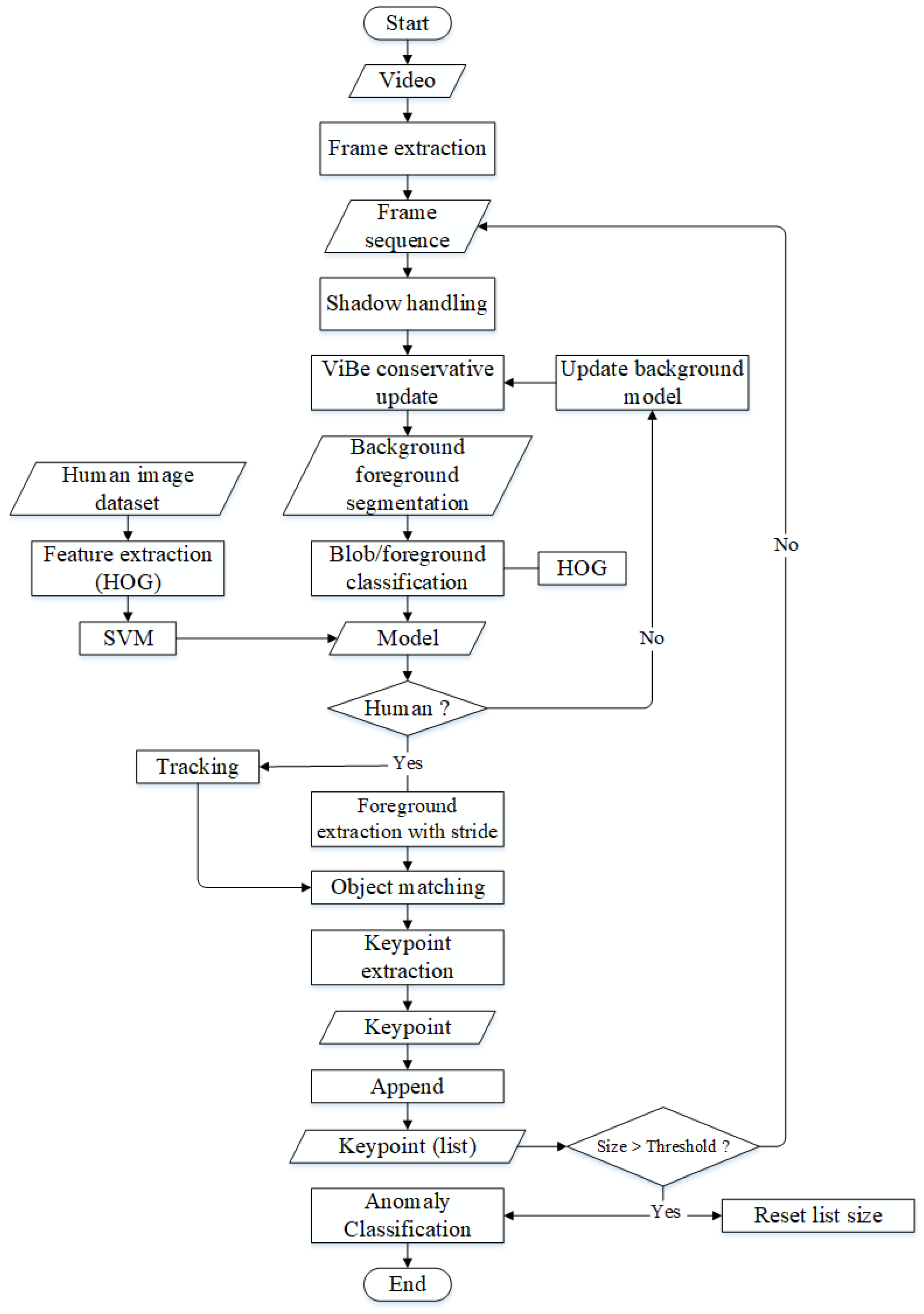
The loitering-detection system starts with video-data acquisition. The video data obtained is extracted into video frames. The video frame is a sequential image. The object shadows on the video frame are removed using a mixture of Gaussian, so as not to affect the background frame modeling results. The background video-modeling process uses the ViBe conservative method. The resulting background model is used for the segmentation process, which results in human objects. Human objects are trained using the histogram of oriented gradient (HOG) method. If a human object is in the video frame, a bounding box will appear, and the tracking process will be carried out. The results of this tracking are in the form of key points from the same human object in video frames. This key point uses the mid-point of the human bounding box. This key point is stored to determine whether the video is normal or abnormal. The angle feature of human steps is used in this study’s analysis. The proposed framework in this research is shown in Figure 1.

2.1. Data Acquisition

In the data acquisition stage, we use two types of data: augmented data and video data. The augmented data describe the movement of objects in a specific time duration to determine whether this object’s movement is an anomaly. An anomaly object represents a human object loitering in a monitoring area. These augmented data are only used for training purposes. In contrast, the second dataset is a collection of video data taken directly using CCTV cameras and shows the movement of humans in various scenarios.

2.1.1. Augmented Data Acquisition for Training

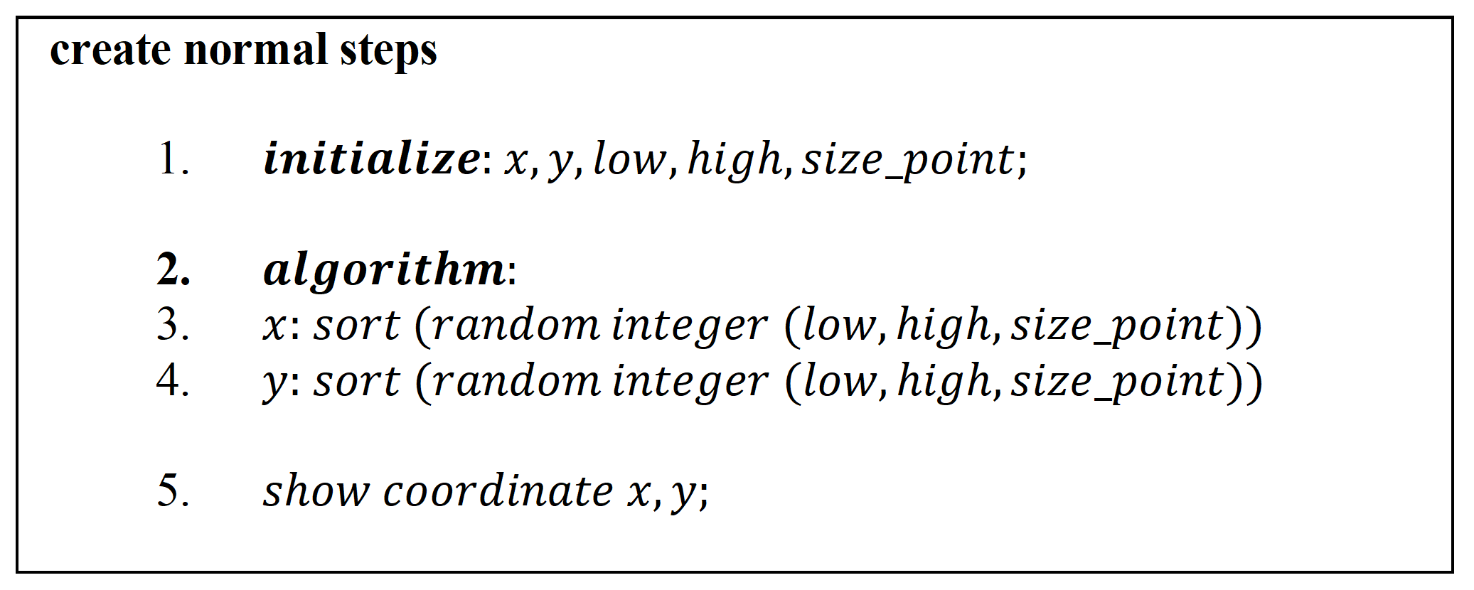
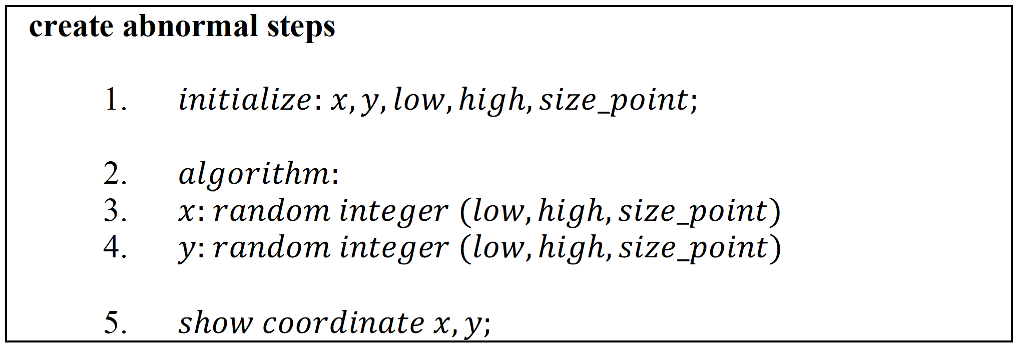
This research uses augmented data which are generated through the program. The augmented data in this research consist of normal and abnormal movement classes. Figure 2 shows the algorithm to get the normal path, while Figure 3 shows the algorithm to get the abnormal path. The number of steps (points) generated in this research was 10, 15, 20, 25, and 30. The data used in this study are 480 in each class, so the total amount of data is 960. The data distribution is 75% for training data and 25% for testing data. The data used for the training process are 720, while the amount for testing is 240.

The step process is obtained by making a simulation with x and y coordinates. A normal movement is a straightforward step or a zigzag in a straight line. In the simulation, as shown in Figure 2, for the program created using the ascending sorting function. This sorting function can be placed on the x or y coordinates or both. The sorting function here is to sequence the steps so that the coordinates appear in the same direction. On the other hand, abnormal movements are back-and-forth motions. 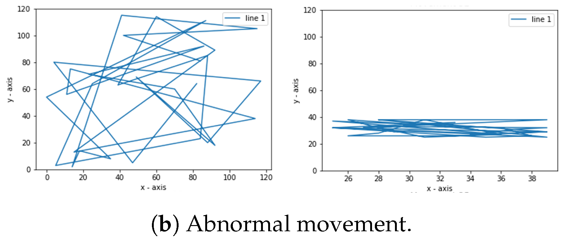In Figure 3, the program does not use the sorting function, which means it only creates random points. Instead, the resulting dots are connected using lines. 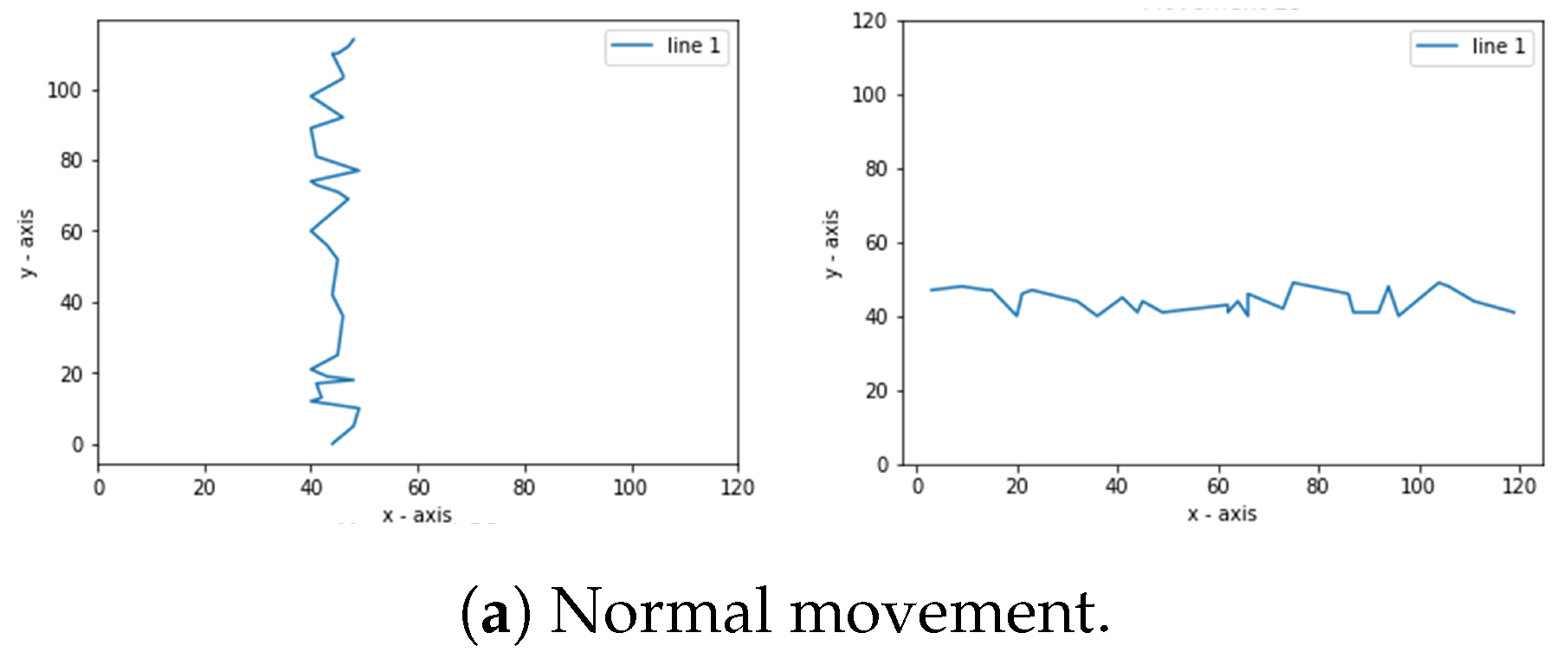Figure 4 shows examples of normal and abnormal steps.

2.1.2. Video Data Acquisition

A total of 20 videos were collected to evaluate the proposed model and features in the testing stage. As many as 7 of the 20 videos contain movements of people who do not loiter, so they are categorized as normal videos. On the other hand, the other 13 videos have scenarios of people loitering in the monitoring area, so those videos are classified as abnormal. The camera used for data collection has full high definition (Full HD) resolution (1080 p) with a 15 fps sampling process. The camera is placed at 2 to 2.5 m in height with a depression angle of 10${}^{\circ }$–45${}^{\circ }$. In detail, the characteristics of each video used in the testing process are shown in

Table 1. Video data description.

Video	Label	Duration (min)	Description
1	Abnormal	00:28	Indoor, narrow room, close object, horizontal zigzag walking object
2	Abnormal	00:34	Indoor, narrow room, close object, vertical zigzag walking object
3	Abnormal	00:20	Indoor, spacious room, distant object, zigzag walking object with minimal displacement
4	Abnormal	00:29	Indoor, large room, distant object, zigzag walking object with minimal displacement
5	Abnormal	00:38	Indoor, large room, close object, vertical zigzag walking object
6	Abnormal	01:03	Outdoor, zigzag moving object when close to camera
7	Abnormal	01:17	Outdoor, objects move zigzag when close to the camera, objects move other objects
8	Abnormal	01:03	Outdoor, diagonal zigzag moving object
9	Abnormal	01:07	Outdoor, objects move zigzag vertically horizontally and diagonally
10	Abnormal	01:07	Outdoor, horizontal vertical zigzag moving object, object crossing obstacle
11	Abnormal	01:06	Outdoor, horizontal vertical zigzag moving object, object crossing obstacle
12	Abnormal	01:02	Outdoor, object moving zigzag horizontally and vertically, object close to camera
13	Abnormal	01:05	Outdoor, object moving zigzag horizontally and vertically, object close to camera
14	Normal	00:13	Indoor, spacious room, distant object
15	Normal	00:21	Indoor, spacious room, close object, object exit towards the stairs
16	Normal	00:19	Indoor, spacious room, close object, object entering through stairs
17	Normal	01:02	Outdoor, horizontal moving object
18	Normal	01:07	Outdoor, moving object combination of horizontal and vertical, object approaching the camera
19	Normal	01:02	Outdoor, the object moves horizontally and vertically, the object moves away from the camera
20	Normal	01:04	Outdoor, horizontal and vertical moving objects, objects close to the camera

.

2.2. Background Modeling

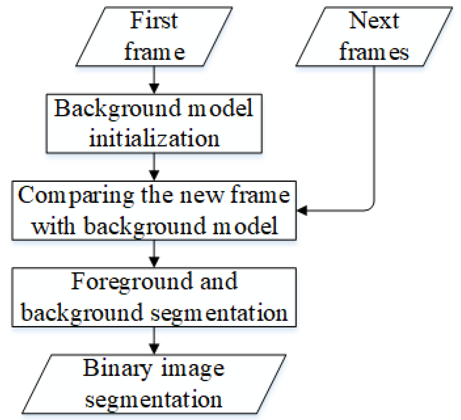
The initial stage of the proposed method is extracting human region candidates from a video. Due to static video characteristics, we may use background modeling to perform this task. The candidate region we will extract is assumed to be a moving human object. Human object movement is detected using ViBe conservative update [11]. This method has three stages: background modeling, comparing new frames with background models, and foreground and background segments. Figure 5 shows a flowchart of the ViBe conservative method. The model of each background pixel is initialized in the first frame. This model contains $N=20$ sample values v taken randomly from the 8-connected region in the pixel. If the background model on the pixel with location x, i.e., $M\left(x\right)$ and $T\left(x\right)$, is the set of neighboring pixels with location x, then $M\left(x\right)$ will contain an Equation (1).

$$\begin{array}{c}\hfill M\left(x\right)=\left\{v\right(y\mid y\in T\left(x\right)\left)\right\}\\ \hfill M\left(x\right)=\{v_1,v_2,\dots ,v_N\}\end{array}$$

(1)

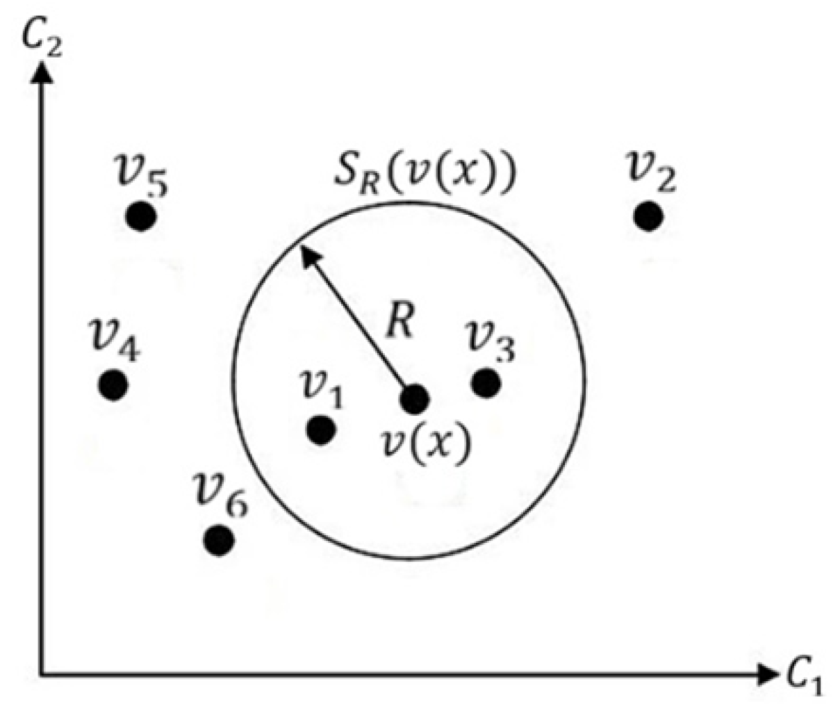
The pixel $v\left(x\right)$ is classified by comparing $M\left(x\right)$ values in the next frame. This comparison is made by defining a circular area $S_R(v\left(x\right)$, which has a radius R and a center point $v\left(x\right)$. An illustration of this stage can be seen in Figure 6.

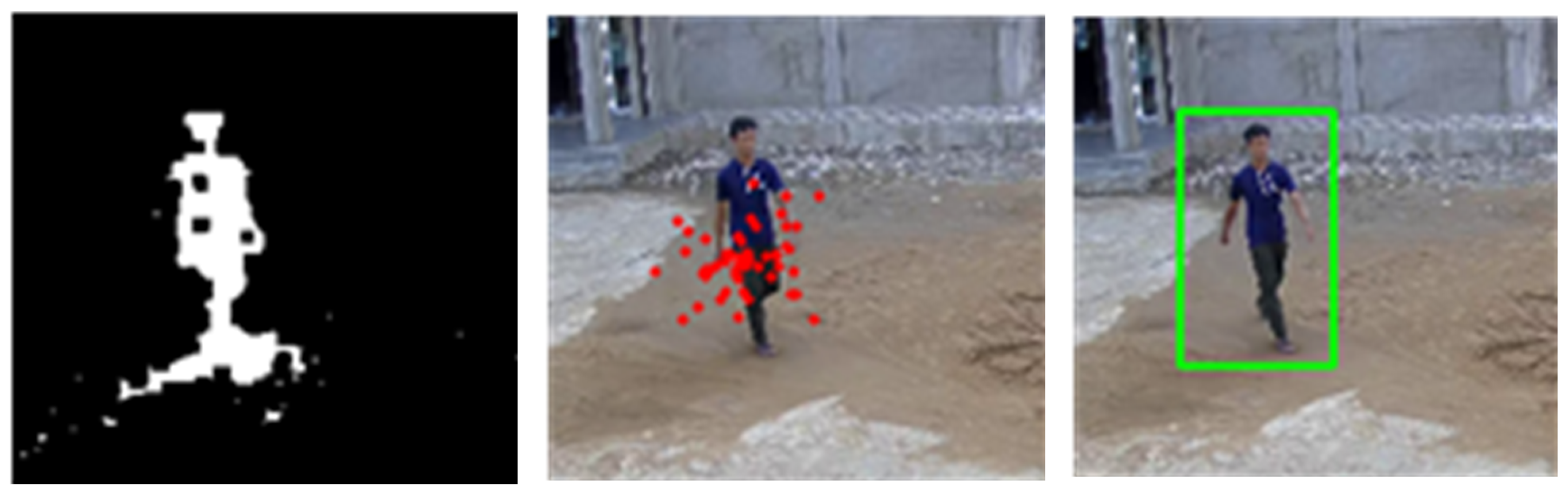
Next, the minimum cardinality $min=2$ threshold value is set. If the number of samples contained in $M\left(x\right)$ from the $S_R\left(v\left(x\right)\right)$ circle area is more significant than #min, then the pixel $v\left(x\right)$ is set as background. If it is smaller, then it is set as foreground. After classifying a pixel as either the background or foreground, the pixel is segmented by giving a value of 0 for the background and 1 for the foreground. Then, the median filtering technique was applied to reduce noise, resulting in a binary image of each frame, with moving objects detected in white while the background is black. 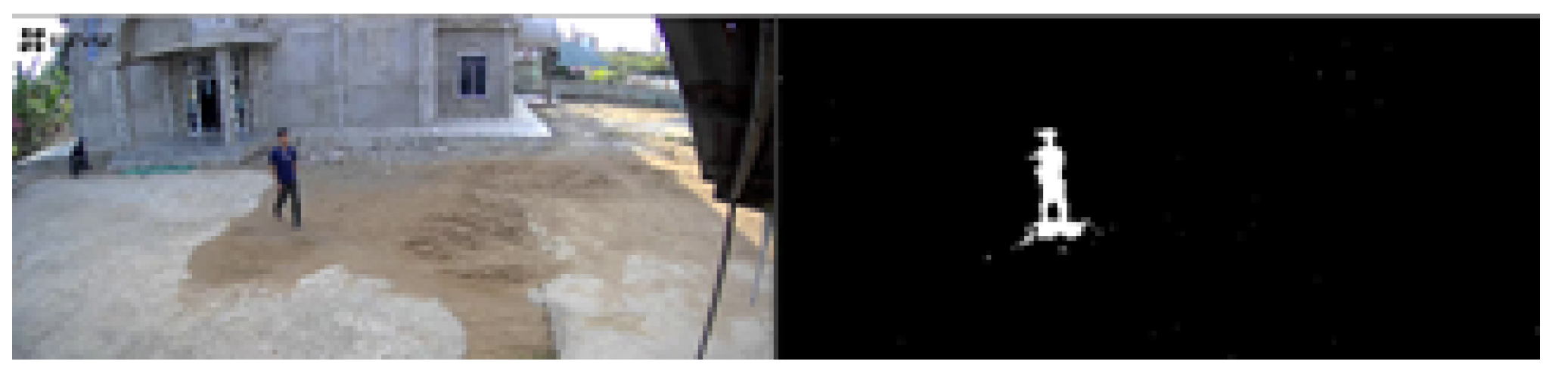Figure 7 shows an example of the segmentation results.

2.3. Human Detection and Tracking

The background modeling method in the previous stage might extract the non-human object region. Therefore, the extracted foreground regions should be verified in the human detection and tracking stage. In this stage, we utilize the classification model of a human object based on the support vector machine (SVM) with the histogram of oriented gradient (HOG) as feature input. Before starting the verification stage, a human image dataset for the training and validation process was prepared, consisting of 665 humans and 665 non-human samples. The human and non-human datasets used in the process were obtained from the image collection of the The Pedestrian Attribute (PETA) dataset [12].

The foreground, classified as a human object, will then be extracted based on the specified stride parameters. The stride parameter is the number of separator frames between two frames containing human foreground at different times. The smaller the value of the stride parameter, the more foreground frames are extracted, and vice versa. In the experiments carried out, the stride parameter used is fps/5.

The tracking method used is tracking by particle filter. There are two steps in tracking using a particle filter: prediction and correction. In performing the two steps, it is necessary to define a target state representation, a dynamic model that describes how the states transition, and an observation model that measures the possibility of new measurements. In this study, the target representation is a foreground object classified as a human. Figure 8 is an example of a tracking particle filter.

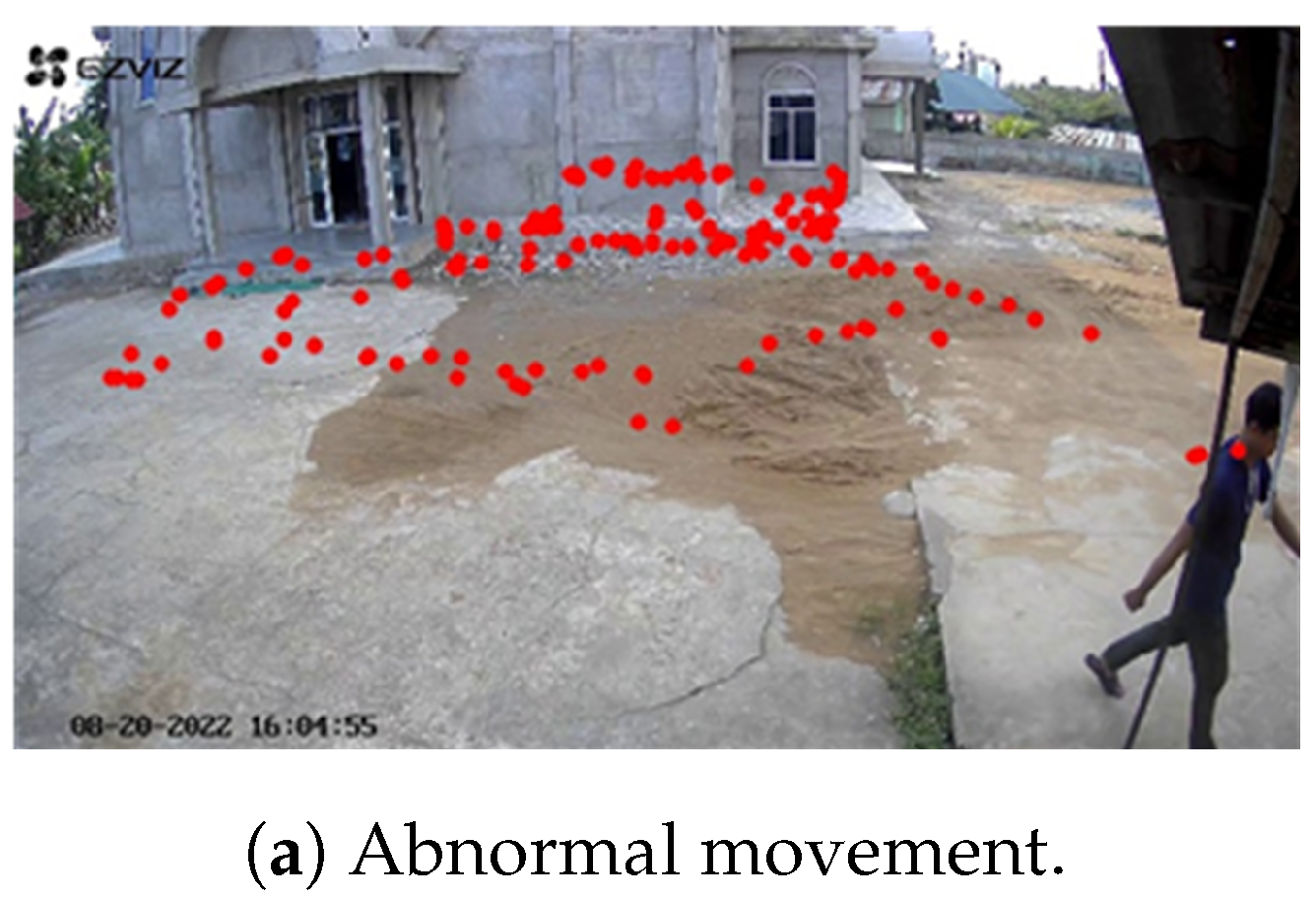
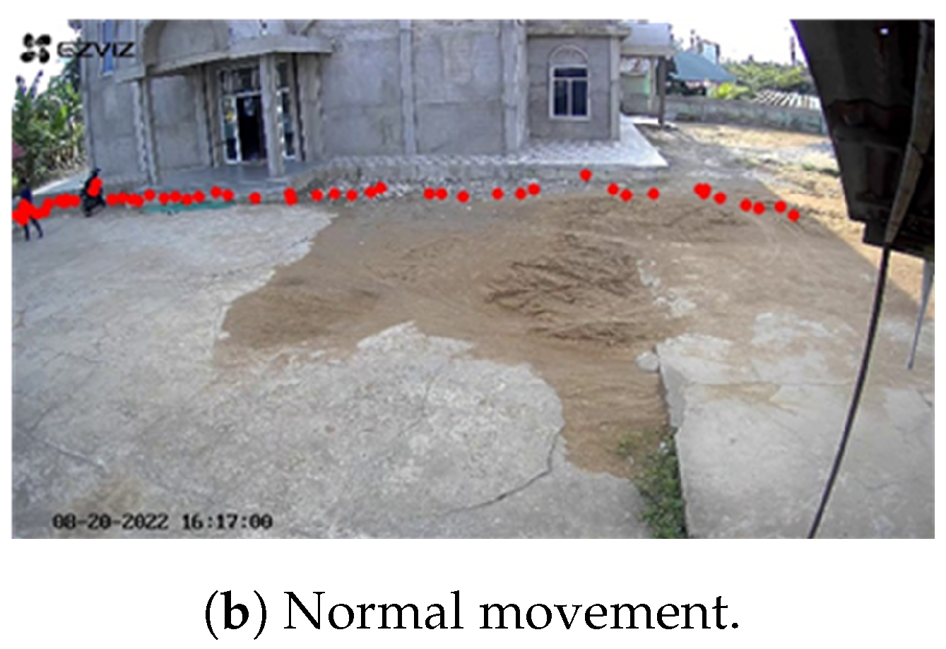
Key point extraction is performed when the similarity value between objects in the bounding box tracking and objects in the bounding box foreground is greater than 80%. Here are some examples of key point extraction results (the extracted key point positions are marked with a red dot). Figure 9 shows an example of the points of detection of both abnormal and normal human movement.

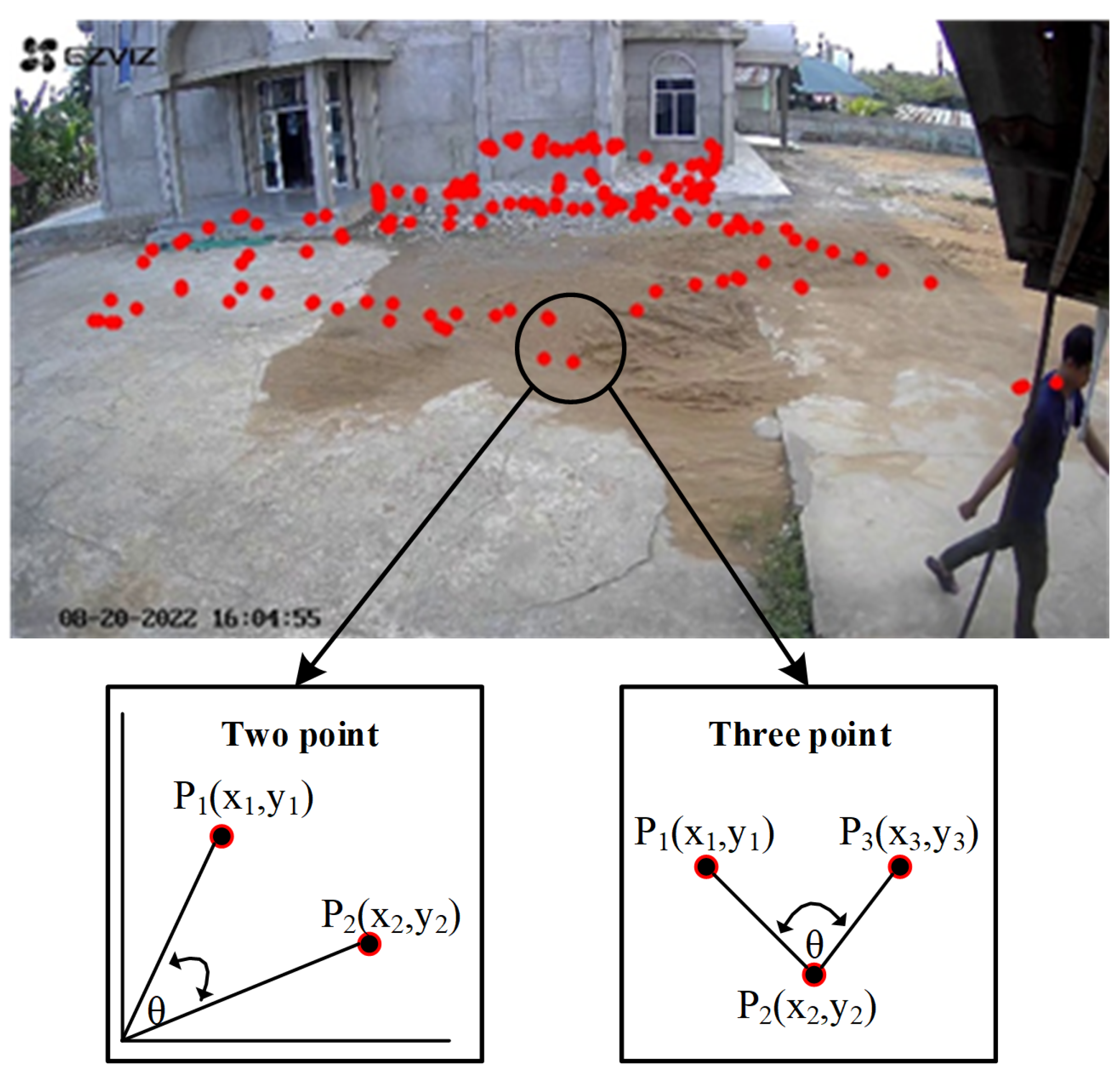
2.4. Spatial-Temporal Feature Extraction

Loitering events are highly dependent not only on the position of the human object in a particular frame, referred to as spatial information, but also on the specific time duration the object appears, defined as temporal information. Therefore, we propose both pieces of information as a novel feature for loitering detection, defined as spatial-temporal features. These features were obtained by calculating the angle at each step. Then, the resulting steps in the video frame are converted into angles. The angle is from $0^{\circ }$ to ${360}^{\circ }$. 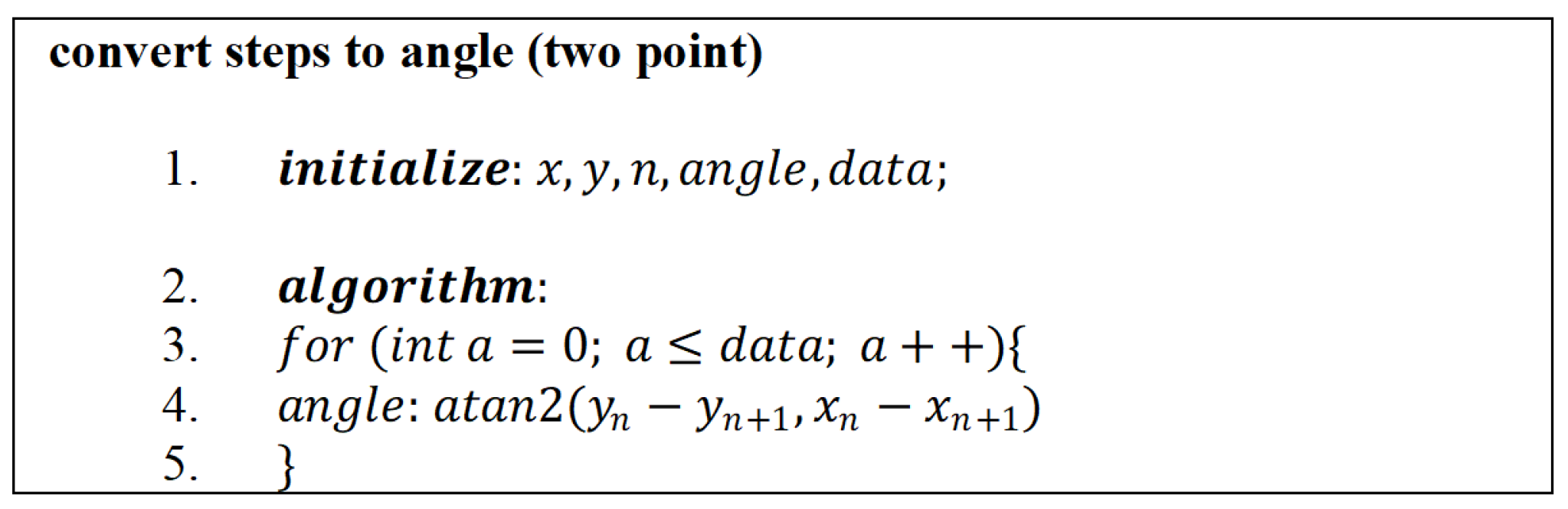The visualization of the point in the step converted into an angle is shown in Figure 10. In this research, the angle is obtained from two or three points. The definition of the tangent of an angle between two points is $delt{a}_y/delt{a}_x$, or $(y_2-y_1)/(x_2-x_1)$. This means that $math.atan2(dy,dx)$ returns the angle between the two locations that constitute the coordinates base of the axis. 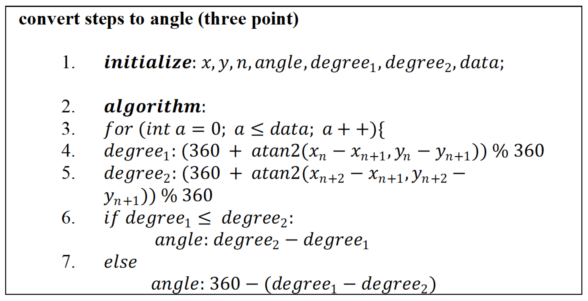Figure 11 shows the algorithm for finding the angles originating from two points. Then, the angle obtained from the three points makes the second angle or $P_2$ axis, $P_1$, and $P_3$ as the endpoint. The algorithm for calculating angles at three points is shown in Figure 12.

The angle results are relatively large, namely 0 to 360. Therefore, the angle is normalized from 0 to 1 to reduce the gap in data. The normalization process is carried out by dividing the angle obtained by 360. The normalization equation is shown in Equation (2).

$$Normalize=\frac{angle}{360}$$

(2)

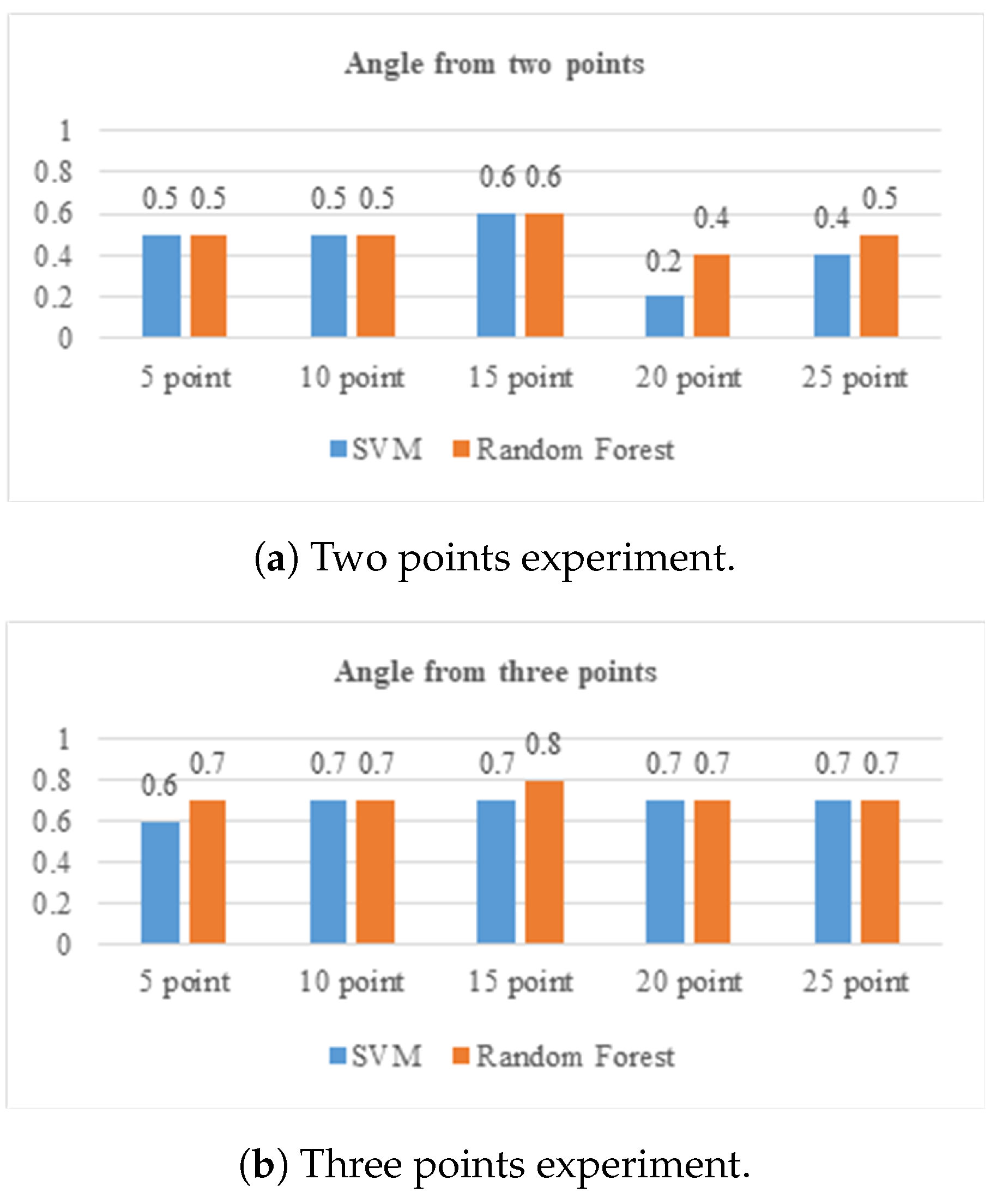
Finally, the final feature will represent the video with 10, 15, 20, or 25 angle values. The extracted feature is then used to classify whether the video is normal or abnormal. This research uses labels $(-1)$ for abnormal and $\left(1\right)$ for normal movements.

2.5. Decision of Loitering Event

In this research, three supervised learning methods will be explored: the k-nearest neighbor [13], support vector machine [14], and random forest [15].

2.5.1. K-Nearest Neighbor

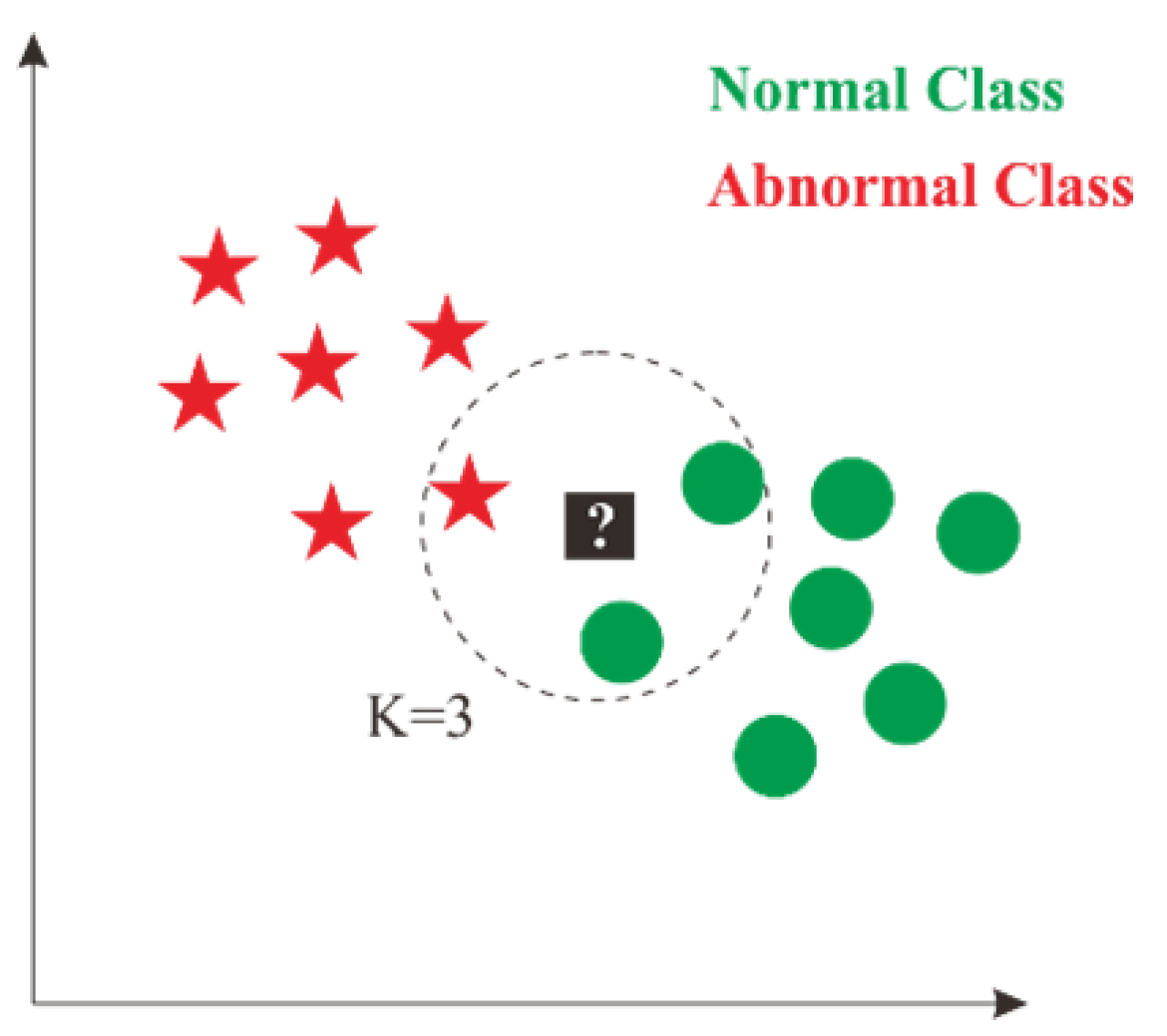
The k-nearest neighbor (KNN) approach classifies objects based on the learning data nearest to the database. KNN is a supervised classification technique in which input data are labeled before training. This technique is utilized frequently in pattern recognition [16,17] and image processing [18]. The data will be projected onto multidimensional spaces, with each dimension representing a data characteristic. This area is separated into categories based on the classification of learning data, including normal and abnormal. Figure 13 illustrates an example of the KNN approach.

2.5.2. Random Forest

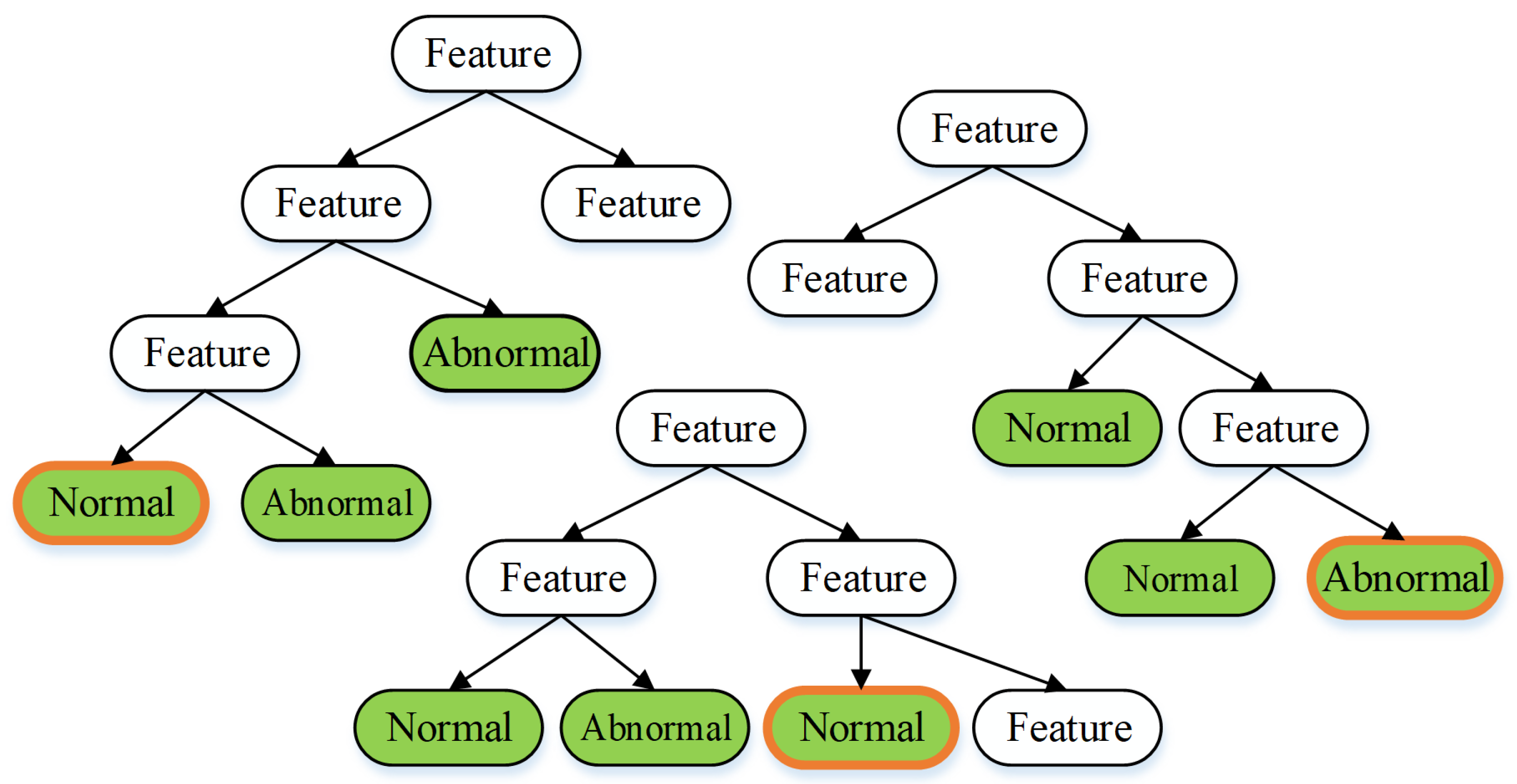
Random forest is a commonly used predictive model method for classification [15]. Random forest generates an arbitrary number of random decision trees. The decision tree includes the characteristics of each class. The decision or categorization procedure is derived from most voting decisions on the decision tree. Then, Figure 14 depicts the application of the random forest approach to the investigation.

In Figure 14, for instance, there are three trees. Then, every node in the tree represents a property of each class. Two normal classes and one abnormal class are derived from the three trees. Hence, it can be inferred that the random forest approach yields the normal class.

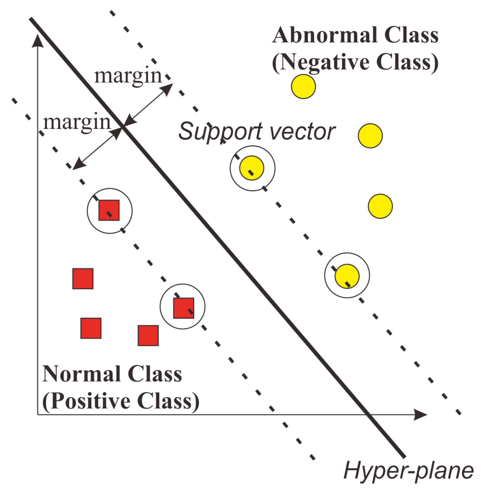
2.5.3. Support Vector Machine

Support vector machine (SVM) is one of the classification techniques commonly employed in supervised learning [14]. By maximizing the distance between classes, SVM is used to discover the optimal hyperplane. The hyperplane is a function that can be utilized to divide classes. The hyperplane discovered by SVM is depicted in Figure 15. The hyperplane is located between the two classes. The hyperplane should maximize the margin between the support vector from each class, as described in red and yellow circles.

3. Results and Discussion

3.1. Experimental Setting and Evaluation Protocols

The experimental process was carried out using a core i5 11400H device with 8 GB of RAM. The programming language used is Python with the library OpenCV [19]. The experiment was carried out by conducting the training process for the angular features using the SVM, KNN, and random forest methods. Finally, the best results are used for trials using video data for the normal or abnormal classification process.

3.2. Optimal Model Selection

3.2.1. Optimal Model Selection of Support Vector Machine

Our first experiment was done by using a support vector machine. In the implementation, we compare the performance of the kernel on SVM, namely the linear kernel, radial basis function kernel, and polynomial kernel [20]. As shown in

Table 2. Experiment with SVM Method.

Kernel	Three Points				Two Points
	Recall	Precision	F1 Score	Accuracy	Recall	Precision	F1 Score	Accuracy
Linear	0.58	0.60	0.57	0.59	0.83	0.83	0.83	0.82
RBF	1.00	1.00	1.00	1.00	0.82	0.84	0.82	0.82
Polynomial	0.93	0.94	0.94	0.93	0.81	0.82	0.80	0.80

, it is found that the Radial Basis Function (RBF) kernel has the best performance among the three kernels. On the other hand, the linear kernel produces the worst accuracy. This happens because the data involved in the training process are non-linear.

In many cases, RBF performs well in handling non-linear data. The results on the polynomial kernel are good, but the implementation requires significant resources and longer computational time than RBF. In addition, using polynomial functions allows for overfitting because our model may fit too much data. Therefore, generalizations may suffer. In contrast, RBF may generalize the data better than polynomials. Therefore, our best model in the support vector was the utilization of the RBF kernel function.

3.2.2. Optimal Model Selection of K-Nearest Neighbor

In the second experiment, we did use a support vector machine. We compare several K values in the implementation, namely 1, 3, 5, and 7. As seen in

Table 3. Experiment with KNN method.

K Value	Three Points				Two Points
	Recall	Precision	F1 Score	Accuracy	Recall	Precision	F1 Score	Accuracy
1	0.82	0.88	0.82	0.82	0.74	0.75	0.75	0.74
3	0.78	0.86	0.78	0.79	0.76	0.76	0.76	0.76
5	0.65	0.81	0.61	0.67	0.79	0.79	0.79	0.79
7	0.63	0.80	0.59	0.65	0.77	0.77	0.77	0.77

, it is found that as the value of K increases, the model decreases in terms of accuracy at three points. On the other hand, the model increases in terms of accuracy when the value of K increases when two points are used. However, the three-point strategy is still better than the two-point strategy. In addition, increasing the value of K will generally increase the computational time during the classification process. So, in the KNN model, we decided to use a value of K = 1 for the three-point strategy.

3.2.3. Optimal Model Selection of Random Forest

Our third experiment is implementing random forest to model the proposed feature. One of the essential hyperparameters in a random forest is the number of trees used. In our experiment, we used various numbers of trees, including 20, 40, 60, and 80. As seen in

Table 4. Experiment with random forest method.

Number of Trees	Three Points				Two Points
	Recall	Precision	F1 Score	Accuracy	Recall	Precision	F1 Score	Accuracy
20	0.98	0.98	0.98	0.97	0.89	0.89	0.89	0.88
40	0.98	0.98	0.98	0.98	0.91	0.91	0.91	0.91
60	0.99	0.99	0.99	0.99	0.92	0.92	0.92	0.92
80	0.98	0.98	0.98	0.98	0.93	0.93	0.93	0.93

, it is found that increasing the number of trees increases the accuracy value obtained by the model. However, there is no significant increase after the number of trees exceeds 80, so we only use the number of trees equal to 80 by considering the computational time required. If we increase the number of trees to more than 80, the computation time will increase, but the accuracy tends to experience only a slight increase.

3.3. Evaluation of Loitering Detection on Video Data

The proposed feature has been modeled in the previous experiment with three popular machine-learning methods. Based on the experimental results, using two points that are converted into angles, the best results are obtained using the SVM and random forest methods. First, the best configuration uses a linear kernel on SVM and a composition of 80 trees on the random forest method. Then, using three points converted to angles, the best results were obtained using the RBF kernel in the SVM method, 60 trees in the random forest method. Therefore, the video data experiment will use this configuration to determine the accuracy of the classification results.

We use as many as 20 videos to evaluate the best model to detect anomalies (loitering) or not in a video. Because the duration of the video and the loitering event can be different, we set the length of the extracted key points in the video with several values of 5, 10, 15, 20, and 25 points. The difference in the length of these points will be evaluated based on the level of accuracy. The video contains two classes of normal and abnormal movement, with five videos in each class. Figure 16 shows the experiment using matched video data on the two- and three-point models. The experimental results show all the best accuracy results from the three-point matching model. The best accuracy is generated at 15 points. Therefore, video testing will use this configuration for experiments using various conditions.

In testing video data, the configuration of the SVM method with RBF kernel and random forest with 60 trees will be carried out. The videos used for this testing process are 20, with 13 actual videos being abnormal and seven actual videos being normal. The results of testing 20 videos are shown in

Table 5. Experiment on video data.

Video	Actual	Prediction
		SVM	Random Forest
1	Abnormal	Abnormal	Abnormal
2	Abnormal	Abnormal	Abnormal
3	Abnormal	Abnormal	Abnormal
4	Abnormal	Normal	Abnormal
5	Abnormal	Abnormal	Abnormal
6	Abnormal	Normal	Abnormal
7	Abnormal	Abnormal	Abnormal
8	Abnormal	Normal	Normal
9	Abnormal	Normal	Normal
10	Abnormal	Abnormal	Abnormal
11	Abnormal	Normal	Normal
12	Abnormal	Abnormal	Abnormal
13	Abnormal	Abnormal	Abnormal
14	Normal	Normal	Normal
15	Normal	Normal	Normal
16	Normal	Normal	Normal
17	Normal	Normal	Normal
18	Normal	Normal	Normal
19	Normal	Normal	Normal
20	Normal	Normal	Normal

. The best results were obtained using the random forest method based on the experimental results. The number of correct predictions is 17, so the accuracy is $85\%$, while in the SVM method, the correct number is only 15, so the accuracy is $75\%$.

3.4. State of the Art Comparison

Finally, the proposed method is also compared with other loitering detection methods, namely the method in Jin Su Kim’s research [5]. The loitering detection method used in Jin Su Kim’s research [5] uses two main features, namely the distance between objects moving between frames (Equation (3)) and the angle resulting from the movement of objects between frames (Equation (4)). Figure 17a shows the method for measuring movement distance of the object.

The object centroid displacement method computes the object displacement distance between frames. The object’s $L(t-1)$ motion from $t-1$ to t is calculated by Equation (3). X is the change in object length. Y is the change in object height. H stands for the object height, which is used to correct incorrect movement distance calculations based on the video and the object’s distance. Figure 17b shows the method for changing the angles of the object.

$$\begin{array}{c}\hfill L(t-1)=\frac{\sqrt{X^2+Y^2}}{H}\end{array}$$

(3)

When an object moves from time $t-2$ to time $t-1$, the angle generated is $(t-1)$, and when it moves from time $t-1$ to time t, the angle created is $\left(t\right)$. The angle is determined using X and Y changes in the centroid of the object. Angle changes are calculated using the difference between $(t-1)$ and $\left(t\right)$. The angles are calculated using Equation (4).

$$\begin{array}{c}\hfill \theta \left(t\right)=arctan\frac{Y}{X}\end{array}$$

(4)

The loitering detection system uses a human step three-point configuration. The parameter configuration for our the best model is shown in

Table 6. Parameter configuration for classifier methods.

Method	Parameter
SVM	RBF kernel
KNN	Value of K = 1
Random forest	Number of trees = 80

. In evaluating this system, the SVM method parameters use the RBF kernel. Then, the KNN method uses parameters with a value of K = 1. Furthermore, the random forest method uses 80 trees as a configuration parameter. The choice of this parameter configuration is based on the experimental analysis results found in Table 2, Table 3 and Table 4. The two features are combined and become the input of the three classifier models used in the proposed feature. By testing using the same data, the difference in accuracy between the feature in [5] and the proposed feature in this study can be seen in

Table 7. Loitering detection method accuracy comparison.

Method	Accuracy in Each Classifer (%)			Average
	SVM	KNN	Random Forest
Distance and angle [5]	65	70	60	65
Proposed method	75	79	85	79.67

.

Table 7 shows that the proposed method produces a higher accuracy value when compared to the method in [5]. The difference in the average accuracy for the three models is 14.67%, with the proposed method being superior. This comparison shows that more features only sometimes result in better accuracy.

3.5. Discussion

From the several experiments conducted, the method produces good accuracy in detecting loitering. Therefore, this method can be integrated into the intelligent surveillance system as a model to detect anomalies in monitoring areas along with detection of fire [21], illegal parking [22], or other anomaly cases [23]. However, the proposed method still has some weaknesses that can be improved in further research.

Firstly, the model fails to detect loitering when the illumination change occurs very quickly, for example, when the weather suddenly turns from sunny to cloudy. The background modeling used has yet to handle this problem, so the resulting region candidates are sometimes imperfect, which causes the determination of key points to be wrong. Furthermore, it will cause the feature extraction process to be irrelevant. Therefore, it is necessary to consider using more robust background modeling technique in handling very fast illumination changes [24,25]. Apart from being based on the appearance of human objects, the use of human skeletons to detect human objects is also seen as more resistant to changes in illumination [26]. In addition, the combination of several sensor devices to detect human objects is also suggested [27].

Second, the proposed model can only be used in the case of videos containing only one person. If the number of people in the video is more than one, using tracking with a particle filter can cause problems during key point extraction, when more than one object is occluded with another. Therefore, the use of tracking also greatly affects results in detecting human loitering. Tracking methods other than particle filters might be considered in further research [28]. It should be noted that the spatial information used in this study is information obtained from 2D images. Thus, it is possible that changes in human poses while walking will affect tracking results; in this case, loitering detection will be also failed. Therefore, spatial information from 3D human objects may also be considered in obtaining spatial information [29].

4. Conclusions

The method for detecting loitering events in a CCTV monitoring area has been implemented. The proposed method was conducted based on spatial and temporal information in the feature extraction stage. Spatial information is obtained by determining the position of the human object in each frame, while temporal information is obtained by looking for the continuity of the position of the human object in consecutive frames. The experimental results show that the combination of spatial and temporal information achieved a relatively good result for detecting loitering.

References

1. Ibrahim, S.W. A comprehensive review on intelligent surveillance systems. Commun. Sci. Technol. 2016, 1, 7–14. [Google Scholar] [CrossRef] [Green Version]
2. Wahyono; Filonenko, A.; Hariyono, J.; Jo, K.-H.; Shahbaz, A.; Kang, H.D. Integrating Multiple Tasks of Vision-based Surveillance System: Design and Implementation. In Proceedings of the 21st Korea-Japan Joint Workshop on Frontiers of Computer Vision (FCV-2016), Takayama Gifu, Japan, 17–19 February 2016; pp. 91–94. [Google Scholar]
3. Kim, D.; Kim, H.; Mok, Y.; Paik, J. Real-time surveillance system for analyzing abnormal behavior of pedestrians. Appl. Sci. 2021, 11, 6153. [Google Scholar] [CrossRef]
4. Patel, A.S.; Vyas, R.; Vyas, O.P.; Ojha, M.; Tiwari, V. Motion-compensated online object tracking for activity detection and crowd behavior analysis. Vis. Comput. 2022, 1–21. [Google Scholar] [CrossRef] [PubMed]
5. Kim, J.S.; Kim, M.G.; Pan, S.B. A study on implementation of real-time intelligent video surveillance system based on embedded module. Eurasip J. Image Video Process. 2021, 2021, 35. [Google Scholar] [CrossRef]
6. Ganapathyraja, R.; Balamurugan, S.P. Suspicious Loitering detection using a contour-based Object Tracking and Image Moment for Intelligent Video Surveillance System. J. Algebr. Stat. 2022, 13, 1294–1303. [Google Scholar]
7. Chen, H.; Bohush, R.; Kurnosov, I.; Ma, G. Detection of Appearance and Behavior Anomalies in Stationary Camera Videos Using Convolutional Neural Networks. Pattern Recognit. Image Anal. 2022, 32, 254–265. [Google Scholar] [CrossRef]
8. Zhang, X.; Yang, S.; Zhang, J.; Zhang, W. Video anomaly detection and localization using motion-field shape description and homogeneity testing. Pattern Recognit. 2020, 105, 107394. [Google Scholar] [CrossRef]
9. Mehmood, A. Abnormal behavior detection in uncrowded videos with two-stream 3d convolutional neural networks. Appl. Sci. 2021, 11, 3523. [Google Scholar] [CrossRef]
10. Asad, M.; Yang, J.; Tu, E.; Chen, L.; He, X. Anomaly3D: Video anomaly detection based on 3D-normality clusters. J. Vis. Commun. Image Represent. 2021, 75, 103047. [Google Scholar] [CrossRef]
11. Barnich, O.; Van Droogenbroeck, M. ViBe: A universal background subtraction algorithm for video sequences. IEEE Trans. Image Process. 2011, 20, 1709–1724. [Google Scholar] [CrossRef] [Green Version]
12. Deng, Y.; Luo, P.; Loy, C.C.; Tang, X. Pedestrian Attribute Recognition At Far Distance. In Proceedings of the 22nd ACM international conference on Multimedia (MM ’14), Orlando, FL, USA, 3–7 November 2014; Association for Computing Machinery: New York, NY, USA, 2014; pp. 789–792. [Google Scholar] [CrossRef]
13. Cover, T.M.; Hart, P.E. Nearest neighbor pattern classification. IEEE Trans. Inf. Theory 1967, 13, 21–27. [Google Scholar] [CrossRef] [Green Version]
14. Cortes, C.; Vapnik, V. Support-vector networks. Mach. Learn. 1995, 20, 273–297. [Google Scholar] [CrossRef]
15. Ho, T.K. Random Decision Forests. In Proceedings of the 3rd International Conference on Document Analysis and Recognition, Montreal, QC, Canada, 14–16 August 1995; pp. 278–282. [Google Scholar]
16. Tamamadin, M.; Lee, C.; Kee, S.-H.; Yee, J.-J. Regional Typhoon Track Prediction Using Ensemble k-Nearest Neighbor Machine Learning in the GIS Environment. Remote Sens. 2022, 14, 5292. [Google Scholar] [CrossRef]
17. Saini, I.; Singh, D.; Khosl, A. QRS detection using K-Nearest Neighbor algorithm (KNN) and evaluation on standard ECG databases. J. Adv. Res. 2013, 4, 331–344. [Google Scholar] [CrossRef] [Green Version]
18. Bistroń, M.; Piotrowski, Z. Comparison of Machine Learning Algorithms Used for Skin Cancer Diagnosis. Appl. Sci. 2022, 12, 9960. [Google Scholar] [CrossRef]
19. Pulli, K.; Baksheev, A.; Kornyakov, K.; Eruhimov, V. Real-Time Computer Vision with OpenCV. Commun. ACM 2012, 55, 61–69. [Google Scholar] [CrossRef]
20. Panja, S.; Chatterjee, A.; Yasmin, G. Kernel Functions of SVM: A Comparison and Optimal Solution. In Advanced Informatics for Computing Research; Luhach, A., Singh, D., Hsiung, P.A., Hawari, K., Lingras, P., Singh, P., Eds.; ICAICR 2018; Communications in Computer and Information Science; Springer: Singapore, 2019; Volume 955. [Google Scholar] [CrossRef]
21. Wahyono; Harjoko, A.; Dharmawan, A.; Adhinata, F.D.; Kosala, G.; Jo, K.-H. Real-Time Forest Fire Detection Framework Based on Artificial Intelligence Using Color Probability Model and Motion Feature Analysis. Fire 2022, 5, 23. [Google Scholar] [CrossRef]
22. Wahyono; Jo, K.-H. Cumulative Dual Foreground Differences For Illegally Parked Vehicles Detection. IEEE Ind. Inform. 2017, 13, 2464–2473. [Google Scholar] [CrossRef]
23. Patrikar, D.R.; Parate, M.R. Anomaly detection using edge computing in video surveillance system: Review. Int. J. Multimed. Inf. Retr. 2022, 11, 85–110. [Google Scholar] [CrossRef]
24. Xu, Y.; Dong, J.; Zhang, B.; Xu, D. Background modeling methods in video analysis: A review and comparative evaluation. CAAI Trans. Intell. Technol. 2016, 1, 43–60. [Google Scholar] [CrossRef] [Green Version]
25. Kim, W.; Jung, C. Illumination-Invariant Background Subtraction: Comparative Review, Models, and Prospects. IEEE Access 2017, 5, 8369–8384. [Google Scholar] [CrossRef]
26. Yu, T.; Jin, H.; Tan, W.-T.; Nahrstedt, K. SKEPRID: Pose and Illumination Change-Resistant Skeleton-Based Person Re-Identification. ACM Trans. Multimed. Comput. Commun. Appl. 2018, 14, 1–24. [Google Scholar] [CrossRef]
27. Shuai, X.; Shen, Y.; Tang, Y.; Shi, S.; Ji, L.; Xing, G. milliEye: A Lightweight mmWave Radar and Camera Fusion System for Robust Object Detection. In Proceedings of the International Conference on Internet-of-Things Design and Implementation, Charlottesvle, VA, USA, 18–21 May 2021; pp. 145–157. [Google Scholar] [CrossRef]
28. Mrabti, W.; Baibai, K.; Bellach, B.; Thami, R.; Tairi, H. Human motion tracking: A comparative study. Procedia Comput. Sci. 2019, 148, 145–153. [Google Scholar] [CrossRef]
29. Sun, J.; Fang, H.-S.; Zhu, X.; Li, J.; Lu, W. Correlation Field for Boosting 3D Object Detection in Structured Scenes. Proc. AAAI Conf. Artif. Intell. 2022, 36, 2298–2306. [Google Scholar] [CrossRef]
Figure 1. The proposed method flowchart.
Jsan 12 00009 g001
Figure 2. Algorithm for generating normal movements.
Jsan 12 00009 g002
Figure 3. Algorithm for generating abnormal movements.
Jsan 12 00009 g003
Figure 4. Movement simulation.
Jsan 12 00009 g004aJsan 12 00009 g004b
Figure 5. Flowchart of the ViBe conservative update.
Jsan 12 00009 g005
Figure 6. Pixel classification using a circular area S R ( v ( x ) ) in a two-dimensional Euclidean color space ( C 1 , C 2 ) .
Jsan 12 00009 g006
Figure 7. Example of moving object segmentation results with the ViBe conservative update.
Jsan 12 00009 g007
Figure 8. Tracking with particle filter.
Jsan 12 00009 g008
Figure 9. Example of normal and abnormal tracking.
Jsan 12 00009 g009aJsan 12 00009 g009b
Figure 10. Angular feature extraction visualization.
Jsan 12 00009 g010
Figure 11. Algorithm for calculating angle from two point.
Jsan 12 00009 g011
Figure 12. Algorithm for calculating angle from three point.
Jsan 12 00009 g012
Figure 13. Illustration of KNN method.
Jsan 12 00009 g013
Figure 14. Illustration of random forest method.
Jsan 12 00009 g014
Figure 15. Illustration of support vector machine.
Jsan 12 00009 g015
Figure 16. Experiment on data video using two and three points.
Jsan 12 00009 g016
Figure 17. Distance and angle measurement used in method [5].
Jsan 12 00009 g017