
Power Distribution of D2D Communications in Case of Energy Harvesting Capability over κ-μ Shadowed Fading Conditions

Abstract
:1. Introduction
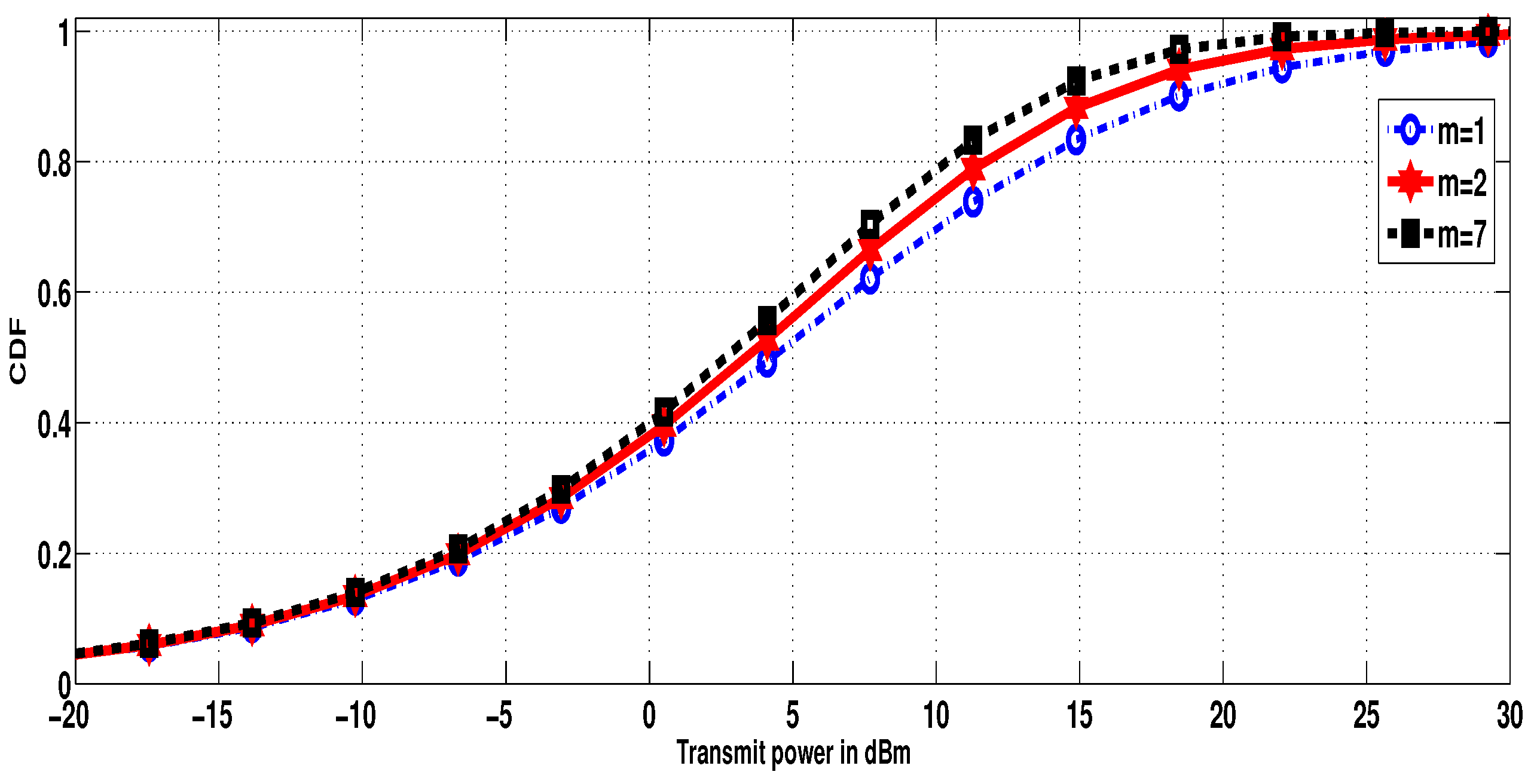
- In the context of D2D underlaid communications, we analyze the SINR at the receiver side when the channel fading is modeled as - shadowed. We then derive the CDF of the required transmission power to achieve the target where the SINR is greater than a threshold.
- Based on the general form of CDF, some particular cases of channel fading, especially Nakagami and Rayleigh fading channels, are also derived. We also derive the transmit power distribution in a noiseless environment.
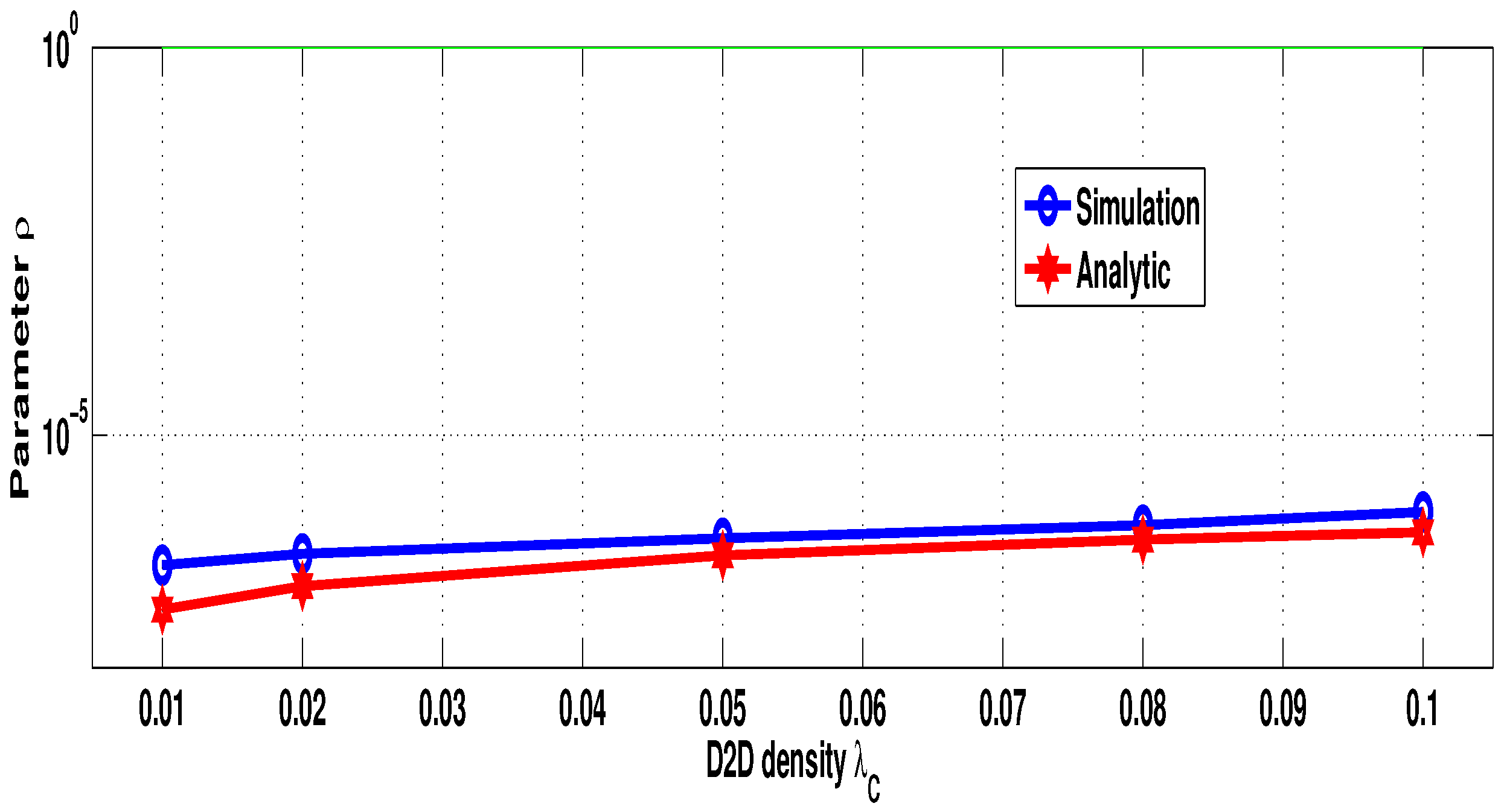
- We consider the case where D2D transmitters are equipped with a radio frequency harvesting system. We assume that the power is gathered from the cellular users’ equipment transmitted energy. Then, we derive the expectation of the harvested energy. In addition, we calculate the expectation of the transmit power of D2D transmitters. Based on this finding, we suggest the probability that a D2D transmitter can achieve its transmission successfully.
- Finally, the accuracy of the analytical results under different fading channel schemes is assessed through an extensive numerical simulation.
2. Related Work
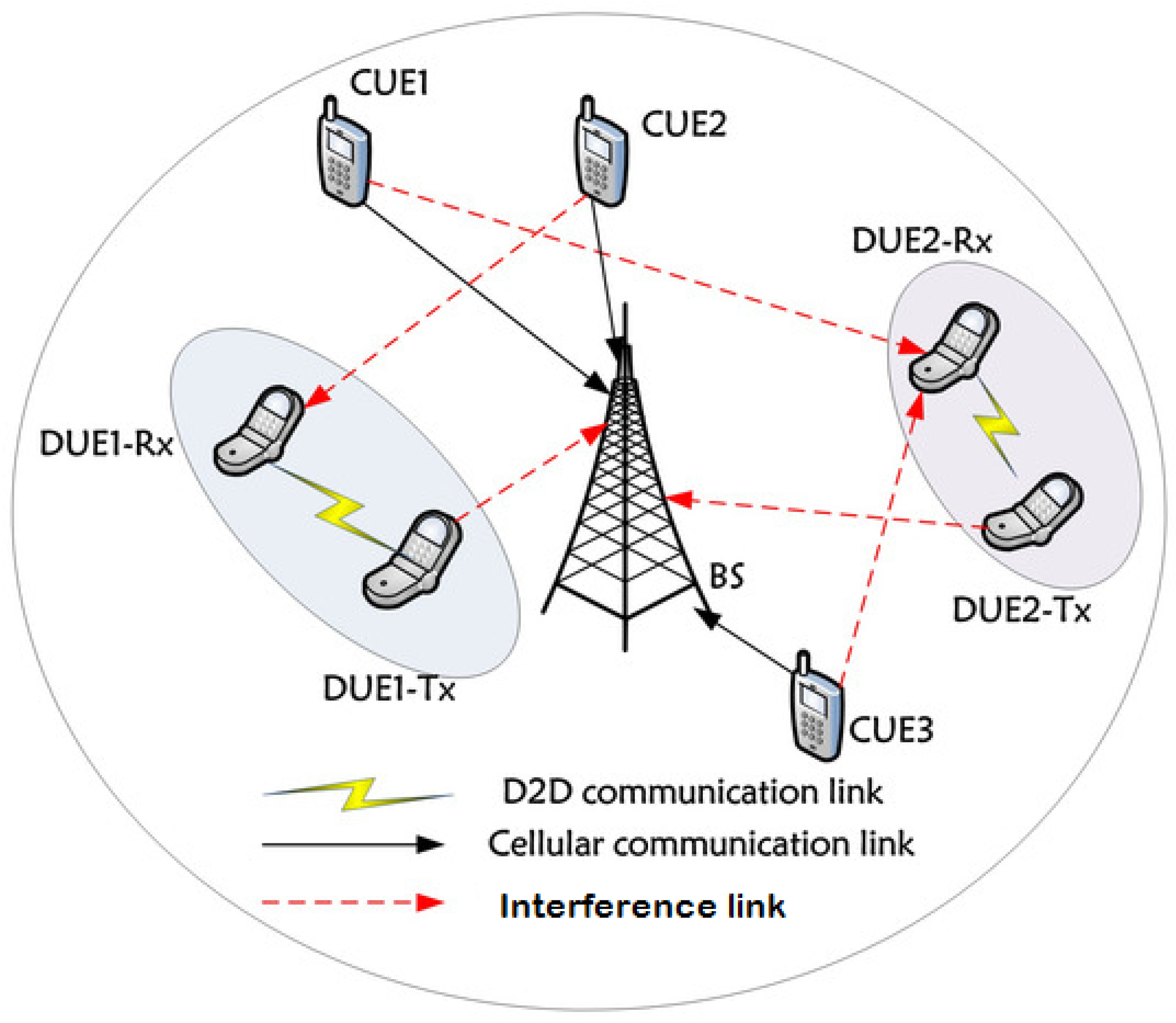
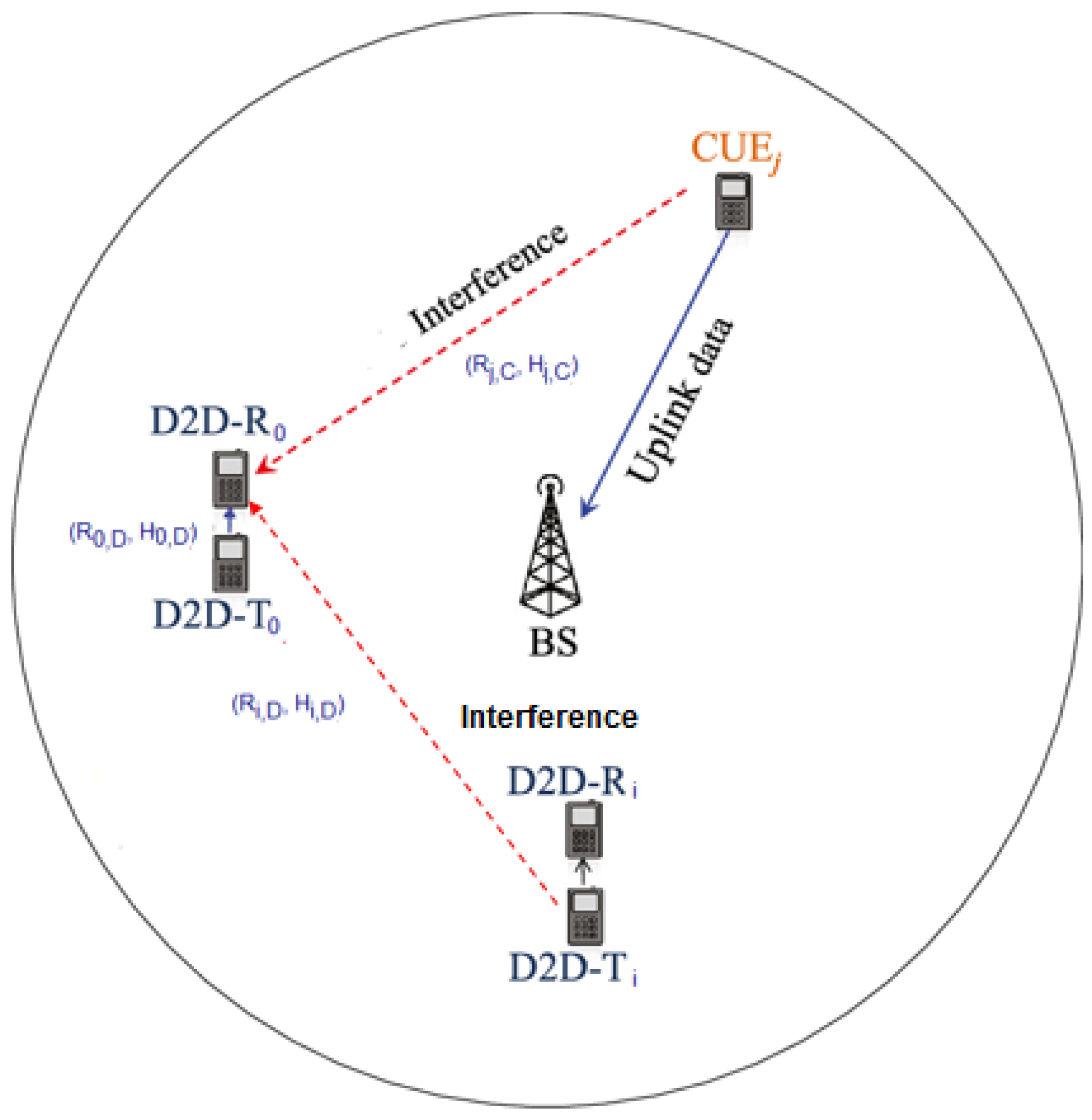
3. System Model
4. CDF of Transmit Power
- There is a circularity in our CDF, in which, depends on the PDF of . Thus, by differentiating (17) and making some variables change, we obtain:
- Based on Table I in [39], we can obtain many distributions. As the - distribution is a special case of a - shadowed distribution (when ), we can easily express our CDF in the case of the - fading environment by putting . We will highlight other special cases in the following corollaries, as they have more closed forms.
5. RF Energy-Harvesting Model
5.1. Expected RF Energy Harvesting Rate
5.2. Energy Utilization Rate
5.3. D2D User Transmission Probability
6. Numerical Study
6.1. Simulation Parameters
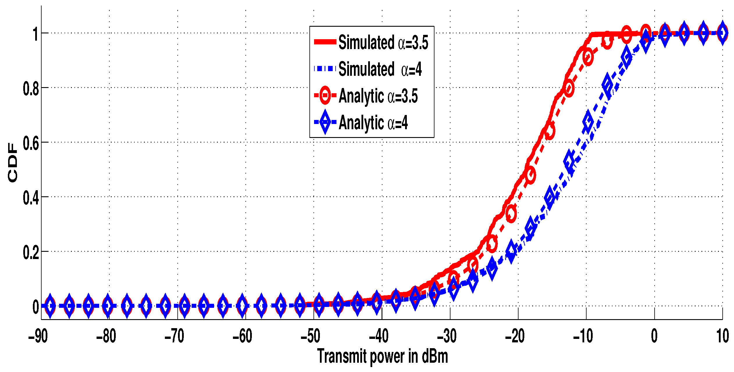
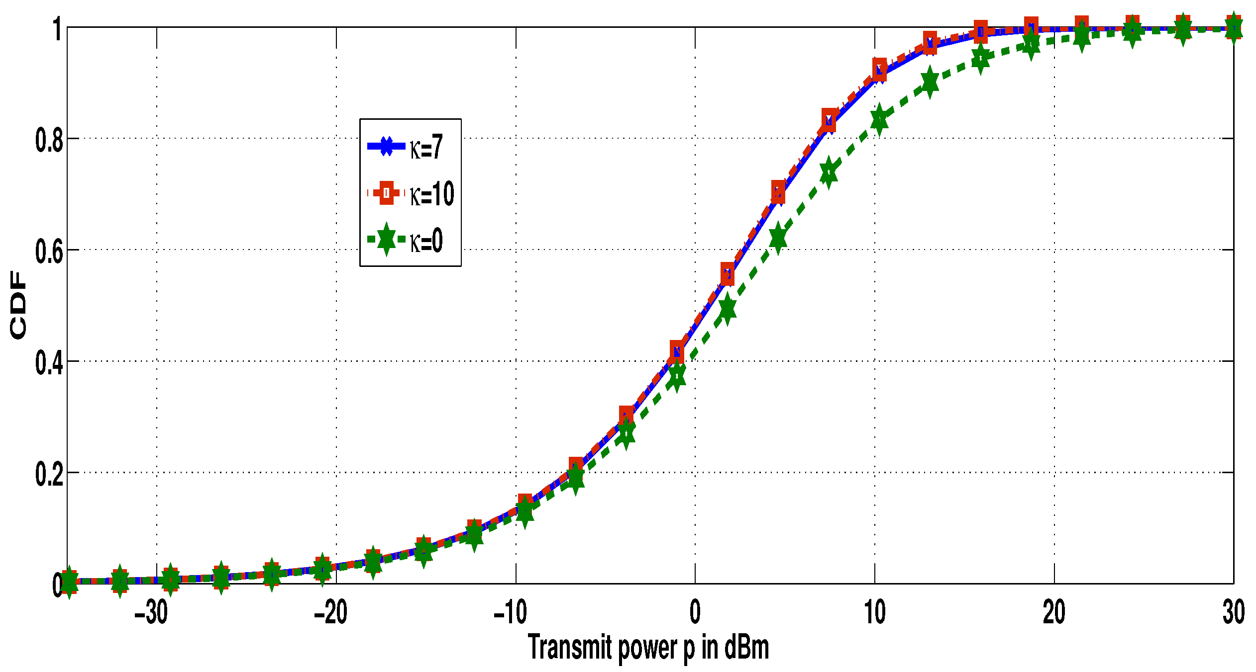
6.2. Results and Discussions
7. Conclusions
Author Contributions
Funding
Institutional Review Board Statement
Informed Consent Statement
Data Availability Statement
Conflicts of Interest
References
- Shafique, K.; Khawaja, B.A.; Sabir, F.; Qazi, S.; Mustaqim, M. Internet of Things (IoT) for Next-Generation Smart Systems: A Review of Current Challenges, Future Trends and Prospects for Emerging 5G-IoT Scenarios. IEEE Access 2020, 8, 23022–23040. [Google Scholar] [CrossRef]
- Porambage, P.; Gur, G.; Osorio, D.P.M.; Liyanage, M.; Gurtov, A.; Ylianttila, M. The roadmap to 6G security and privacy. IEEE Open J. Commun. Soc. 2021, 2, 1094–1122. [Google Scholar] [CrossRef]
- Kar, U.N.; Sanyal, D.K. An overview of device-to-device communication in cellular networks. ICT Express 2018, 4, 203–208. [Google Scholar] [CrossRef]
- Alnoman, A.; Anpalagan, A. On D2D communications for public safety applications. In Proceedings of the 2017 IEEE Canada International Humanitarian Technology Conference (IHTC), Toronto, ON, Canada, 21–22 July 2017; pp. 124–127. [Google Scholar] [CrossRef]
- Goratti, L.; Steri, G.; Gomez, K.M.; Baldini, G. Connectivity and security in a D2D communication protocol for public safety applications. In Proceedings of the 2014 11th International Symposium on Wireless Communications Systems (ISWCS), Barcelona, Spain, 26–29 August 2014; pp. 548–552. [Google Scholar] [CrossRef]
- Liu, J.; Kato, N.; Ma, J.; Kadowaki, N. Device-to-Device Communication in LTE-Advanced Networks: A Survey. IEEE Commun. Surv. Tutor. 2014, 17, 1923–1940. [Google Scholar] [CrossRef]
- Han, L.; Zhang, Y.; Zhang, X.; Mu, J. Power Control for Full-Duplex D2D Communications Underlaying Cellular Networks. IEEE Access 2019, 7, 111858–111865. [Google Scholar] [CrossRef]
- Wen, S.; Zhu, X.; Lin, Z.; Zhang, X.; Yang, D. Energy Efficient Power Allocation Schemes for Device-to-Device(D2D) Communication. In Proceedings of the 2013 IEEE 78th Vehicular Technology Conference (VTC Fall), Las Vegas, NV, USA, 2–5 September 2013; pp. 1–5. [Google Scholar] [CrossRef]
- Bulashenko, A.; Piltyay, S.; Demchenko, I. Energy Efficiency of the D2D Direct Connection System in 5G Networks. In Proceedings of the 2020 IEEE International Conference on Problems of Infocommunications. Science and Technology (PIC S&T), Kharkiv, Ukraine, 6–9 October 2020; pp. 537–542. [Google Scholar] [CrossRef]
- Nguyen, K.K.; Duong, T.Q.; Vien, N.A.; Le-Khac, N.-A.; Nguyen, M.-N. Non-Cooperative Energy Efficient Power Allocation Game in D2D Communication: A Multi-Agent Deep Reinforcement Learning Approach. IEEE Access 2019, 7, 100480–100490. [Google Scholar] [CrossRef]
- Doan, T.X.; Hoang, T.M.; Duong, T.Q.; Ngo, H.Q. Energy Harvesting-Based D2D Communications in the Presence of Interference and Ambient RF Sources. IEEE Access 2017, 5, 5224–5234. [Google Scholar] [CrossRef]
- Sun, P.; Shin, K.G.; Zhang, H.; He, L. Transmit Power Control for D2D-Underlaid Cellular Networks Based on Statistical Features. IEEE Trans. Veh. Technol. 2017, 66, 4110–4119. [Google Scholar] [CrossRef]
- Paris, J.F. Statistical Characterization of κ-μ Shadowed Fading. IEEE Trans. Veh. Technol. 2014, 63, 518–526. [Google Scholar] [CrossRef]
- Goswami, A.; Kumar, A. Statistical Characterization and Performance Evaluation of α-η-μ/Inverse Gamma and α-κ-μ/Inverse Gamma Channels. Wirel. Pers. Commun. 2022, 124, 2313–2333. [Google Scholar] [CrossRef]
- Ramirez-Espinosa, P.; Moualeu, J.M.; da Costa, D.B.; Lopez-Martinez, F.J. The α-κ-μ Shadowed Fading Distribution: Statistical Characterization and Applications. In Proceedings of the 2019 IEEE Global Communications Conference (GLOBECOM), Big Island, HI, USA, 9–13 December 2019. [Google Scholar]
- Hunukumbure, M.; Moulsley, T.; Oyawoye, A.; Vadgama, S.; Wilson, M. D2D for energy efficient communications in disaster and emergency situations. In Proceedings of the 2013 21st International Conference on Software, Telecommunications and Computer Networks—(SoftCOM 2013), Split-Primosten, Croatia, 18–20 September 2013; pp. 1–5. [Google Scholar] [CrossRef]
- Anamuro, C.V.; Varsier, N.; Schwoerer, J.; Lagrange, X. Simple modeling of energy consumption for D2D relay mechanism. In Proceedings of the 2018 IEEE Wireless Communications and Networking Conference Workshops (WCNCW), Barcelona, Spain, 15–18 April 2018; pp. 231–236. [Google Scholar] [CrossRef]
- Shang, B.; Zhao, L.; Chen, K.-C.; Chu, X. Energy Efficient D2D-Assisted Offloading with Wireless Power Transfer, GLOBECOM 2017. In Proceedings of the 2017 IEEE Global Communications Conference, Singapore, 4–8 December 2017; pp. 1–6. [Google Scholar] [CrossRef]
- Amiri, M.H.Z.; Nazemi, A.M.; Namazi, M.; Amri, K.J.; Amiri, F.Z. Energy Saving in D2D Cellular 6G Networks. In Proceedings of the 2020 10th International Conference on Computer and Knowledge Engineering (ICCKE), Mashhad, Iran, 29–30 October 2020; pp. 676–682. [Google Scholar] [CrossRef]
- Zytoune, O.; Fouchal, H.; Zeadally, S. A realistic relay selection scheme for cooperative MIMO networks. Ad Hoc Netw. 2022, 124, 102706. [Google Scholar] [CrossRef]
- Atat, R.; Liu, L.; Mastronarde, N.; Yi, Y. Energy Harvesting-Based D2D-Assisted Machine-Type Communications. IEEE Trans. Commun. 2017, 65, 1289–1302. [Google Scholar] [CrossRef]
- Lu, X.; Wang, P.; Niyato, D.; Kim, D.I.; Han, Z. Wireless Networks With RF Energy Harvesting: A Contemporary Survey. IEEE Commun. Surv. Tutor. 2015, 17, 757–789. [Google Scholar] [CrossRef]
- Atat, R.; Chen, H.; Liu, L. Fundamentals of spatial RF energy harvesting for D2D cellular networks. In Proceedings of the 2016 IEEE Global Communications Conference (GLOBECOM), Washington, DC, USA, 4–8 December 2016; pp. 1–6. [Google Scholar]
- Zungeru, A.M.; Ang, L.-M.; Prabaharan, S.R.S.; Seng, K.P. Radio frequency energy harvesting and management for wireless sensor networks. In Green Mobile Devices and Networks; Venkataraman, H., Muntean, G.-M., Eds.; CRC Press: Boca Raton, FL, USA, 2012; Chapter 13; pp. 341–368. [Google Scholar]
- Lee, S.; Zhang, R.; Huang, K. Opportunistic wireless energy harvesting in cognitive radio networks. IEEE Trans. Wirel. Commun. 2013, 12, 4788–4799. [Google Scholar] [CrossRef]
- Yang, H.H.; Lee, J.; Quek, T.Q.S. Heterogeneous cellular network with energy harvesting-based D2D communication. IEEE Trans. Wirel. Commun. 2016, 15, 1406–1419. [Google Scholar] [CrossRef]
- Wang, Y.; Liu, Y.; Wang, C.; Li, Z.; Sheng, X.; Lee, H.G.; Chang, N.; Yang, H. Storage-less and converter-less photovoltaic energy harvesting with maximum power point tracking for internet of things. IEEE Trans. Comput.-Aided Design Integr. Circuits Syst. 2016, 35, 173–186. [Google Scholar] [CrossRef]
- Zeb, H.; Gohar, M.; Ali, M.; Rahman, A.U.; Ahmad, W.; Ghani, A.; Choi, J.-G.; Koh, S.-J. Zero Energy IoT Devices in Smart Cities Using RF Energy Harvesting. Electronics 2023, 12, 148. [Google Scholar] [CrossRef]
- Luo, Y.; Pu, L.; Lei, L. Impact of Varying Radio Power Density on Wireless Communications of RF Energy Harvesting Systems. IEEE Trans. Commun. 2021, 69, 1960–1974. [Google Scholar] [CrossRef]
- Oulcaid, M.; El Fadil, H.; Njili, S.; Zytoune, O.; Bajit, A. Experimental Implementation of a Wireless Communication System for Electric Vehicle WPT Charger. E3S Web Conf. 2022, 351, 01006. [Google Scholar] [CrossRef]
- Sun, C.; Alemseged, Y.D.; Tran, H.N.; Harada, H. Transmit Power Control for Cognitive Radio Over a Rayleigh Fading Channel. IEEE Trans. Veh. Technol. 2010, 59, 1847–1857. [Google Scholar] [CrossRef]
- Erturk, M.C.; Mukherjee, S.; Ishii, H.; Arslan, H. Distributions of Transmit Power and SINR in Device-to-Device Networks. IEEE Commun. Lett. 2013, 17, 273–276. [Google Scholar] [CrossRef]
- Banagar, M.; Maham, B.; Popovski, P.; Pantisano, F. Power Distribution of Device-to-Device Communications in Underlaid Cellular Networks. IEEE Commun. Lett. 2016, 5, 204–207. [Google Scholar] [CrossRef] [Green Version]
- Boumaalif, A.; Zytoune, O. Power Distribution of Device-to-Device Communications Under Nakagami Fading Channel. IEEE Trans. Mob. Comput. 2022, 21, 2158–2167. [Google Scholar] [CrossRef]
- ElHalawany, B.M.; Jameel, F.; da Costa, D.B.; Dias, U.S.; Wu, K. Performance Analysis of Downlink NOMA Systems Over κ-μ Shadowed Fading Channels. IEEE Trans. Veh. Technol. 2020, 69, 1046–1050. [Google Scholar] [CrossRef]
- Lopez-Martinez, F.J.; Paris, J.F.; Romero-Jerez, J.M. The κ-μ Shadowed Fading Model With Integer Fading Parameters. IEEE Trans. Veh. Technol. 2017, 66, 7653–7662. [Google Scholar] [CrossRef]
- Schilcher, U.; Toumpis, S.; Haenggi, M.; Crismani, A.; Brandner, G.; Bettstetter, C. Interference Functionals in Poisson Networks. IEEE Trans. Inf. Theory 2016, 62, 370–383. [Google Scholar] [CrossRef]
- Andrews, J.G.; Baccelli, F.; Ganti, R.K. A Tractable Approach to Coverage and Rate in Cellular Networks. IEEE Trans. Commun. 2011, 59, 3122–3134. [Google Scholar] [CrossRef]
- Moreno-Pozas, L.; Lopez-Martinez, F.J.; Paris, J.F.; Martos-Naya, E. The κ-μ Shadowed Fading Model: Unifying the κ-μ and η-μ Distributions. IEEE Trans. Veh. Technol. 2016, 65, 9630–9641. [Google Scholar] [CrossRef]
- Drayson Technologies. RF Energy Harvesting for the Low Energy Internet of Things. 2015, pp. 1–7. Available online: http://www.getfreevolt.com (accessed on 8 May 2012).
- Powell, M.J.D. A Fortran Subroutine for Solving Systems of Nonlinear Algebraic Equations. In Numerical Methods for Nonlinear Algebraic Equations; Rabinowitz, P., Ed.; Gordon and Breach: London, UK, 1970; Chapter 7. [Google Scholar]
- Stoyan, D.; Kendall, W.; Mecke, J. Stochastic Geometry and Its Applications, 3rd ed.; John Wiley & Sons: Hoboken, NJ, USA, 2013. [Google Scholar]
- Foschini, G.J.; Miljanic, Z. A Simple Distributed Autonomous Power Control Algorithm and its Convergence. IEEE Trans. Veh. Technol. 2002, 42, 641–646. [Google Scholar] [CrossRef]


| Paper | Cellular/D2D Frequency Band | Channel Fading | Contribution |
|---|---|---|---|
| Sun et al. [31] | Ad hoc networks | Rayleigh | Transmit power CDF |
| Erturk et al. [32] | different | Rayleigh | Transmit power CDF and SINR |
| Banagar et al. [33] | same | Rayleigh | Transmit power CDF |
| Boumaalif et al. [34] | same | Nakagami | Transmit power CDF and device lifetime |
| Our present work | same | - shadowed | Transmit power CDF and user transmit probability in case of energy harvesting |
| Abbreviation | Signification |
|---|---|
| D2D | Device-to-Device |
| CDF | Cumulative Distribution Function |
| RF-EH | Radio Frequency Energy Harvesting |
| IoT | Internet of Things |
| CSI | Channel State Information |
| LOS | Line-Of-Sight |
| SINR | Signal to Interference plus Noise Ratio |
| PPP | Poisson Point Processes |
| Probability Density Function | |
| CCDF | Complementary Cumulative Distribution Function |
| PGFL | Probability Generating Functional |
| Variable | Signification |
|---|---|
| The location of cellular equipments following independent homogeneous PPP | |
| The location of D2D equipments following independent homogeneous PPP | |
| The intensity of | |
| The intensity of | |
| H | The fading power |
| The PDF of H | |
| The CCDF of H | |
| The typical D2D transmitter transmit power | |
| The fading power in the typical D2D communication channel | |
| The distance between the typical D2D transmitter and receiver | |
| The received power in the typical D2D link | |
| The interference caused by the other D2D transmitters to the typical D2D receiver | |
| The interference caused by all cellular transmitters to the typical D2D receiver | |
| The at the typical D2D receiver | |
| The noise power | |
| T | The minimum threshold |
Disclaimer/Publisher’s Note: The statements, opinions and data contained in all publications are solely those of the individual author(s) and contributor(s) and not of MDPI and/or the editor(s). MDPI and/or the editor(s) disclaim responsibility for any injury to people or property resulting from any ideas, methods, instructions or products referred to in the content. |
© 2023 by the authors. Licensee MDPI, Basel, Switzerland. This article is an open access article distributed under the terms and conditions of the Creative Commons Attribution (CC BY) license (https://creativecommons.org/licenses/by/4.0/).
Share and Cite
Boumaalif, A.; Zytoune, O.; El Fadil, H.; Saadane, R. Power Distribution of D2D Communications in Case of Energy Harvesting Capability over κ-μ Shadowed Fading Conditions. J. Sens. Actuator Netw. 2023, 12, 16. https://doi.org/10.3390/jsan12010016
Boumaalif A, Zytoune O, El Fadil H, Saadane R. Power Distribution of D2D Communications in Case of Energy Harvesting Capability over κ-μ Shadowed Fading Conditions. Journal of Sensor and Actuator Networks. 2023; 12(1):16. https://doi.org/10.3390/jsan12010016
Chicago/Turabian StyleBoumaalif, Adil, Ouadoudi Zytoune, Hassan El Fadil, and Rachid Saadane. 2023. "Power Distribution of D2D Communications in Case of Energy Harvesting Capability over κ-μ Shadowed Fading Conditions" Journal of Sensor and Actuator Networks 12, no. 1: 16. https://doi.org/10.3390/jsan12010016