1. Introduction
Mobile nodes that use Wireless Sensor Networks (WSNs) have increased significantly in recent years, due to the fact that mobile applications and their usage play a vital role in many sectors. A Mobile Ad Hoc Network (MANET) is a special type of WSNs which is defined as a collection of independent mobile nodes (mobile devices, laptops, Personal Digital Assistants (PDAs), etc.) that have the ability of exchanging information wirelessly without the need for fixed infrastructures, such as access points, switches or routers [
1]. Due to the frequent physical changes of the topological infrastructure, mobile nodes must perform all the network activities on their own, including the discovery of a network topology, the process of building their own routing tables and the process of managing updates or sending control messages among nodes, as well as the capability of sending, receiving and forwarding information between nodes, i.e., in this case mobile nodes inherit the router operations to forward connection requests between nodes in a distributed fashion [
2,
3]. Mobile nodes have limited resources such as small memory, tiny power resource, limited bandwidth links and low processing power. Because the links are established wirelessly, data transmission over MANETs is vulnerable to high packet losses and more frequent path disconnections compared to wired networks. These issues might also degrade the reliability of the network in delivering data traffic. Mobile nodes that are in a radio range of other nodes can establish a direct communication link, otherwise they cooperate with intermediate nodes to manage the connection. MANETs have many interesting applications that fulfill human needs. Examples of such applications are military fields, emergency situations and natural disasters, etc. In such applications, it is extremely impossible to rely on fixed infrastructures due to their absence or their high implementation costs [
4,
5].
Routing information in MANETs is a big issue, and puts several challenges to researchers on how to design suitable routing protocols to handle them. Therefore, many routing protocols have been developed that are compatible with the characteristics and the dynamic nature of these networks. Existing routing protocols have their own design mechanisms to improve some of the MANET performance metrics. Among the most important metrics are throughput, Packet Delivery Ratio (PDR), routing overhead and end-to-end delay [
5,
6]. These metrics are interrelated and interdependent; this means that working to improve one often leads to negatively affecting others.
Routing protocols in MANETs are broadly classified into three categories: proactive, reactive or hybrid [
7,
8]. In proactive-based routing, every node manages its own routing table/s to store the routing information for all connected nodes. To keep the routing information constantly updated, the nodes exchange update messages frequently or periodically. This method makes routing information available whenever needed, but at the same time, increases routing overhead. Examples of this category are Fisheye State Routing protocol (FSR) [
9] and Optimized Link State Routing protocol (OLSR) [
10].
In reactive protocols, the nodes do not retain routing information—instead, they broadcast route requests to the destination node on demand. This step is only performed when data routing is required, which increases the throughput, but also increases the end-to-end delay. Ad Hoc On-demand Distance Vector (AODV) [
11] and Dynamic Source Routing (DSR) [
12] are well-known routing protocols belonging to this category.
Hybrid protocols like Zone Routing Protocol (ZRP) [
13] and Temporally-Ordered Routing Algorithm (TORA) [
14] utilize the positive characteristics of both mechanisms (proactive and reactive) to improve the performance of the routing process.
Due to the permanent movement of the nodes, their connections’ links are continuously broken. All the metrics mentioned above are affected by the age of the links established between nodes. This means that the path duration between any source-destination communication’s link might affect the performance metrics of the routing protocols. In the case the path duration is too long, there is greater throughput, greater PDR and lower routing overhead and vice versa. The path duration mainly depends on three parameters: speed of the node, direction of movement, and range of transmission signals.
Destination Sequenced Distance Vector (DSDV) [
15,
16] is a well-known MANET routing protocol, which has been extensively used by the researchers to enhance its performance. Many recent extended versions of this protocol were developed, such as Proactive Routing Protocol for Multi-Channel Wireless Ad Hoc Networks (DSDV-MC) [
17], Hash-MAC-DSDV [
18], Intelligent Promising Support DSDV (IPS DSDV) [
19] and others are appearing on the horizon. It is a proactive loop-free distance vector routing protocol where the nodes periodically forward data packets based on their routing information. Upon receiving the data, the neighboring nodes update their routing tables accordingly. In this case, the required updates will be inserted into the routing table in various settings, e.g., when any required information for a specific destination is missing from the routing table, when the current update message contains a larger sequence number or when the update message with a similar sequence number contains a shorter connection path (smaller hop count). A new update in the routing table will be instantly forwarded to the neighboring nodes and the routing information will be periodically rebroadcast again to reach the convergence state.
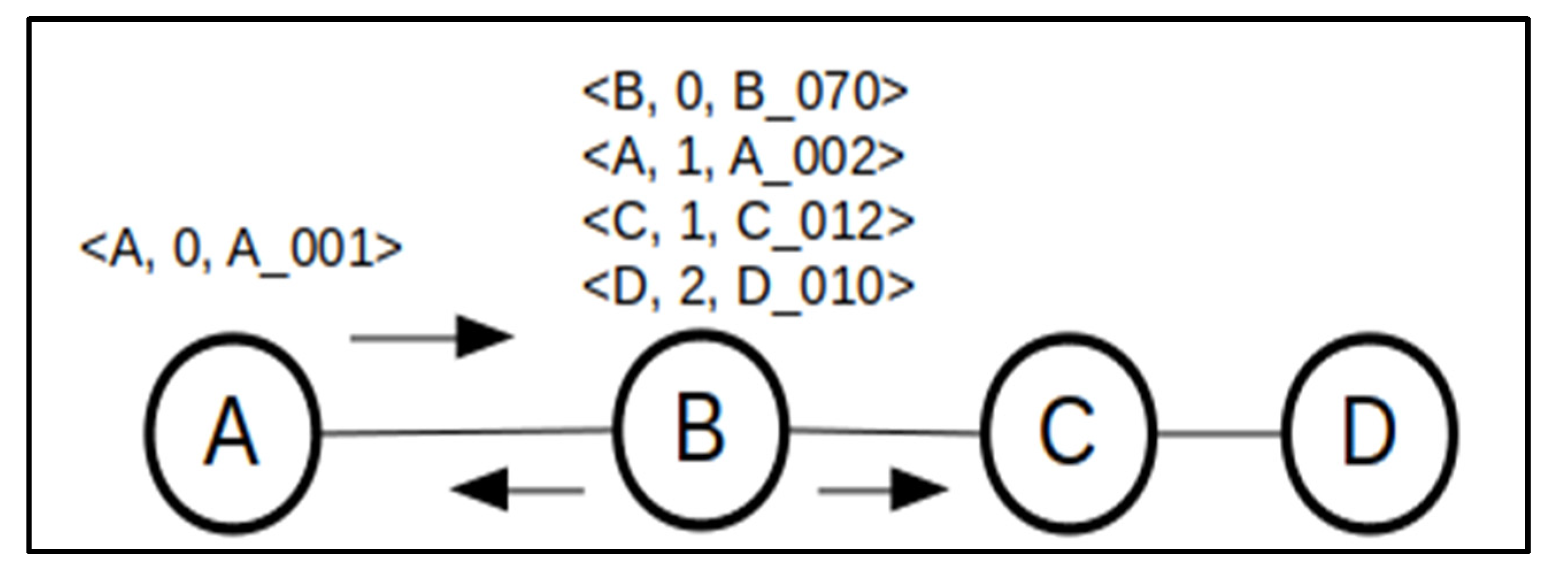
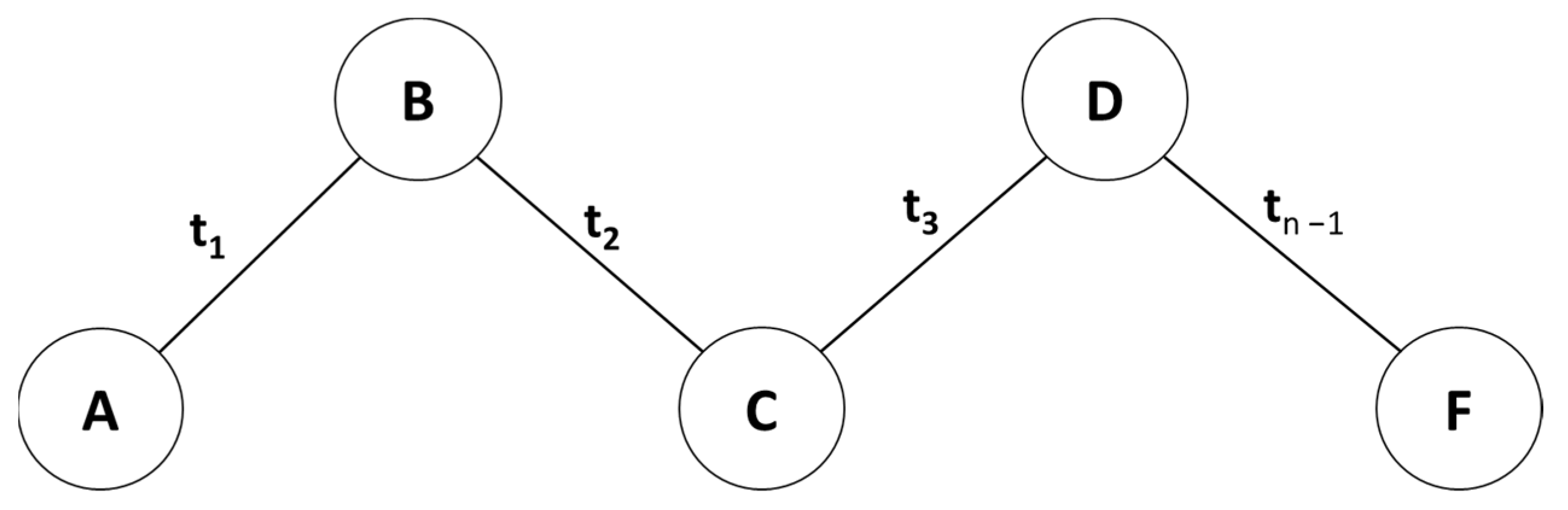
Figure 1 shows an example scenario of this process.
In this scenario, node (A) represents a new device that joined the network recently, so the routing table of node (A) shows only its routing information. All nodes periodically exchange the contents of their routing tables, and each record in the table contains the identity of the node, the number of hops and the sequence number of the record. When node (B) receives the updates from node (A), it increases the hop count to the destination by 1, and adds the new updates to its routing table. In the next periodic update, node (B) forwards its updated routing table to the other neighbors.
The DSDV routing table contains the following five fields:
- -
Next hop: refers to the next node to be visited along the path from the source to the final destination.
- -
Metric: represents the number of nodes involved in packets’ forwarding along the path from the source to the destination.
- -
Sequence number: a unique identifier given to each update message to distinguish between new and old updates.
- -
Settling time: the amount of elapsed time set by the node before broadcasting the incoming updates (this timer will be reset for each update).
- -
Hold down time: the amount of time that determines the lifetime of the record, i.e., marking the record as expiry to consider broken connection.
Since the link and path durations play a crucial role in designing high-efficiency routing protocols, this is mainly due to their direct impact on throughput, end-to-end delay and routing overhead; having their values estimated in advance for a given network scenario can help in the optimal selection of other network parameters such as Time to Live (TTL)—a predetermined value that controls the lifetime of a given packet—and an optimal packet length, which minimizes the overall packet loss. However, the prediction of these durations for a given path is a challenging issue, as the estimation process mainly depends on several dynamic parameters such as node velocity, node direction, network size and number of nodes. Furthermore, due to the mobility nature of MANETs, the connectivity graph may change frequently, i.e., active links which are currently available might not be available at other times. This might affect the useful link and path durations, as well as the overall efficiency of the routing protocol. As a consequence, it is necessary for the routing process to find the best alternative route as soon as the route becomes unavailable due to node mobility. Therefore, building a mathematical model of the protocol can give a quick and easy impression of the performance of the protocol in specific circumstances, but when a deeper analysis of the protocol is required, the need for simulation programs still exists.
Existing models cited in the literature studied this problem for the reactive routing category. In this study, we targeted proactive routing and analyzed one of its main protocols, called the DSDV. Thus, we have built a mathematical-based model to analyze the link and path durations of this protocol to find the best approximated values in real scenarios, which in turn can give a good indication of the factors that might affect its performance.
Besides the introduction section, the remaining parts of the paper are structured as follows: A review of the related work is discussed in
Section 2. In
Section 3, we thoroughly detail the proposed mathematical model and discuss the main assumptions. The validation analysis of the model along the simulation results are provided in
Section 4. Finally, in
Section 5, we derive the conclusion and provide some future works.
2. Related Work
Although the routing process in MANETs is very hot research area, it is clearly shown in the literature that the majority of the contributions used simulation testbeds to implement and validate the developed routing protocols, compared to the mathematical models that have been developed so far. Existing mathematical models examined some of the reactive routing protocols that have adopted very specific conditions to build the mathematical models and this is due to the fact that the adoption of a mathematical model that considers all MANET’s factors make the mathematical model very complex. A brief description of each model is given below.
Patel, et al. [
20] proposed a new statistical-based scheme named Least-Square Quadratic Polynomial Regression-Based-Link Failure (LSQPR-LFE) to estimate the link failure time in MANETs. It builds an optimal error quadratic model between packet arrival time and node distance considering signal levels of the delivered packets. The link failure time was calculated by obtaining the moment at which the maximum communication range will be reached. Several simulations scenarios were implemented to test the accuracy of the proposed scheme, considering various mobility models, node density and node velocity. In their proposed model, Namuduri, K. and Pendse, R. [
21] analyzed the path duration using three parameters: node speed, signal level and node density. The main assumption is that the next hop is selected using a function of the Least Remaining Distance (LRD) to the final destination.
Sharm, et al. [
22] proposed a routing protocol called Route Stability-based QoS routing (RSQR) to estimate the probability of link failures based on two parameters: node mobility and signal strength. It determines mobility speeds and relative positions of nodes without requiring any geographical information for nodes. It first uses the signal strength values from the MAC sublayer to compute link stability. Next, it uses less control overhead without enforcing a periodic pilot packet exchange to compute link stability values. Tilwari, et al. [
23] developed a new a routing scheme titled Mobility, Residual energy, and Link quality Aware Multipath (MRLAM) to address the potential drawbacks of MANETs in the areas of link quality, battery consumption and mobility nature. In this routing scheme, a Q-Learning algorithm was implemented to manage the process of selecting the optimal set of intermediate nodes based on link quality, mobility and energy level parameters of a given scenario, positive and negative rewards are assigned to each node accordingly. Compared to other routing protocols, the proposed routing scheme showed a significant improvement in the overall performance in terms of consumed energy, end-to-end delay, packet loss ratio and convergence time. Shelly, et al. [
24] analyzed path and link lifetime in one-dimensional vehicle wireless networks. They assumed a uniform distribution of velocity and lognormal headway distance. The study analyzed the effect of mobility of the vehicles and the transmission range on the average lifetime of the link. They also performed the Kolmogorov-Smirnov test to find the best PDF fits for the link duration. The results have shown that the PDF of link duration can be estimated to be lognormal.
Pal, et al. [
25] conducted some experiments on two exiting statistical models: Autoregressive Integrated Moving Average (ARIMA); and multilayer perceptron (MLP) to predict the path length between a transmitter-receiver pair. They applied three different mobility models to collect path length data: the Random Way Point mobility model (RWP); the Manhattan Grid Mobility Model (MHG); and the Reference Point Group Mobility Model (RPGM). AODV routing protocol was used to evaluate the accuracy of the statistical models. The results showed that MLP-based neural network models outperform the ARIMA model in prediction accuracy. Yadav, et al. [
26] developed a prediction method to estimate the link availability based on the signal strength. using the Newton divided difference method. In this method, each node determines its links’ breakage time, and forwards this information to other nodes in advance. Based on this information, the route discovery process will be initiated earlier to find alternate routes. The proposed approach was implemented on AODV routing protocol. Compared to the generic AODV, the results of the new proposal showed that packet loss and average end-to-end delay were significantly reduced and data packet delivery ratio was increased.
Srinivasan, M. [
27] suggested an analytical model to estimate the average path duration in multihop routing using the Random Way Point (RWP) model. This work considered the node density as a network parameter and studied its impact on the path duration. The results have shown that the average path duration can be analytically predicted for the shortest path routing. Moreover, they showed that the analytical prediction of the average path duration parameter is beneficial in optimizing the routing functionalities such as TTL of a given routing protocol. Carofiglio, et al. [
28] conducted a study to examine the duration probability and availability of routing paths that are subjected to frequent disconnections and link failures caused by the mobility nature of mobile nodes. This study specifically focused on the scenarios where the mobile nodes move according to the RWP model and derived the approximate and actual expressions of these probabilities to select the optimal routes in terms of path availability. It also proposed an approach to find the best routes of reactive routing protocols to improve the efficiency and reduce the routing overhead.
Triviño-Cabrera, et al. [
29] developed an analytical model to predict both the link duration and the path duration in multi-hop WSNs. The developed model was tested using 50 simulation scenarios with various transmission and mobility conditions on two simulation platforms (NS2 and MATLAB). They found out that both the predicted and measured results are consistent with the simulation results estimated by the analytical equations derived from the analytical model. Sakhaee, et al. [
30] developed a new routing algorithm to increase the link duration, improve routing stability and reduce the overall control overhead in high-mobility MANET scenarios. Compared to the existing reactive routing protocols, which consider only disjoint paths, a new discovery concept called non-disjoint paths was introduced in this approach. This study also introduced an approach to find the best estimation of the link lifetime without the need for Global Positioning System (GPS) services. The new approaches were simulated and the traffic overhead analysis showed good performance with promising results.
Bai, et al. [
31] developed another approach to examine the effect of some path duration statistics (PDFs) that vary according to some network parameters such as relative node speed, hop count, transmission range and mobility model. The obtained results argued that at low mobility speeds, some mobility models may induce multimodal distributions that affect some characteristics such as mobility constraints, spatial map and traffic pattern, while at moderate to high velocities, the exponential distribution can provide good path duration approximation for a number of mobility models. Farheen, N. S. and Jain, A. [
32] proposed a hybrid location-based prediction model to estimate the probable locations of mobile nodes with respect to their neighborhoods based on spatial and temporal characteristics. They developed a multi-path routing protocol considering the estimated probability of nodes’ locations with path diversion, in order to improve the routing performance and reduce packets’ overhead.
In summary, to the best of the authors’ knowledge, mathematical modeling of proactive routing protocols to estimate the link and path durations are at developing stages. Moreover, existing mathematical models targeted a small set of factors that directly affect the process of estimating the path duration; this is because including all factors increases the complexity of constructing the mathematical models. Therefore, in this research study, we proposed a mathematical-based model for estimating the link and path durations and studied their effects on the performance of the DSDV routing protocol—one of the main highly deployed proactive routing protocols. We thoroughly described this model on a step-by-step basis, and verified its validity by doing a comparative analysis between the simulation results and the predicted values derived from the mathematical model.
4. Model Analysis and Discussion
To validate the proposed mathematical-based model and study the effect of the DSDV protocol on its path duration estimation, we have built two simulation scenarios (
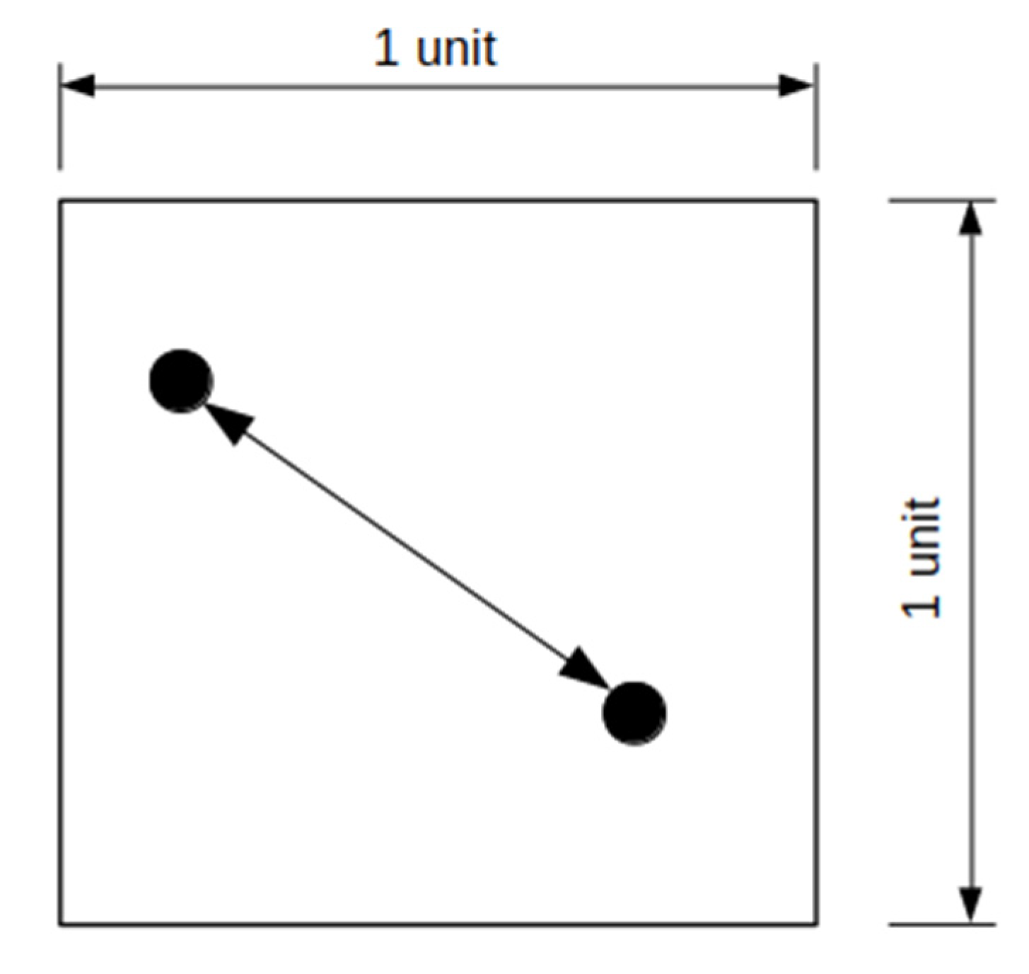
Table 1). In the first scenario, we selected a simulation area of 1000 × 1000 m
2 and the node’s signal range of 250 m and the mobility of the nodes and their velocities are selected using the RWP model. The velocity of each step is increased by 5 m/s, (5, 10, 15, …). In the second scenario, we kept the scenario dimension as in the first one (1000 × 1000 m
2), and fixed the nodes’ velocities at 10 m/s. The distribution of the movement of the nodes are kept random. The initial value of the signal range is 100 m, and this increases by 10 m in each step. The change in the signal range means a change in the hop count, which is needed to reach the destination node. Meanwhile, the node with a short-range signal requires more hops to reach the destination node.
Table 1 summarizes these settings.
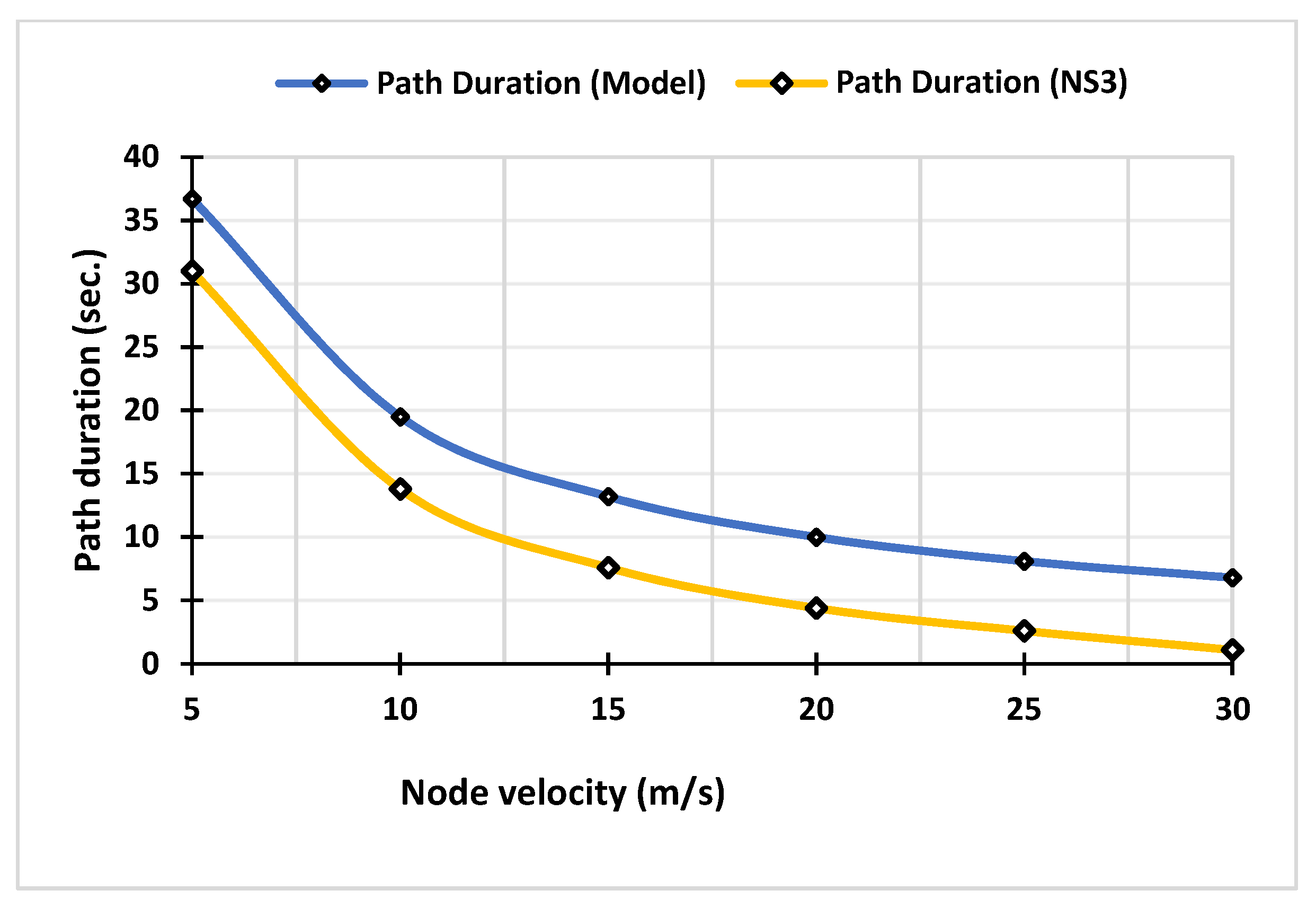
Figure 9 illustrates the relationship between the node velocity and the path duration. It is observed that the path duration decreases with the increase in the node’s speed, and it is significantly reduced when the speed exceeds 10 m/s. It is also noted that the actual path duration is longer than the DSDV path duration, and this difference increases by increasing the nodes’ velocity.
Furthermore, we found out that the analysis of the DSDV path duration is less than the actual path duration, since the DSDV protocol needs to wait for a time period (settling time) before rebroadcasting the routing information. During the waiting period, the nodes keep moving, and consequently the path duration of the DSDV protocol will be decreased.
The nodes that install the DSDV instance periodically update their routing information. In the case the interval between the current and next update periods is longer than the path duration to the final destination, the node loses the connection to the destination node before the routing information is updated. Thus, the period between both update intervals is not fully utilized.
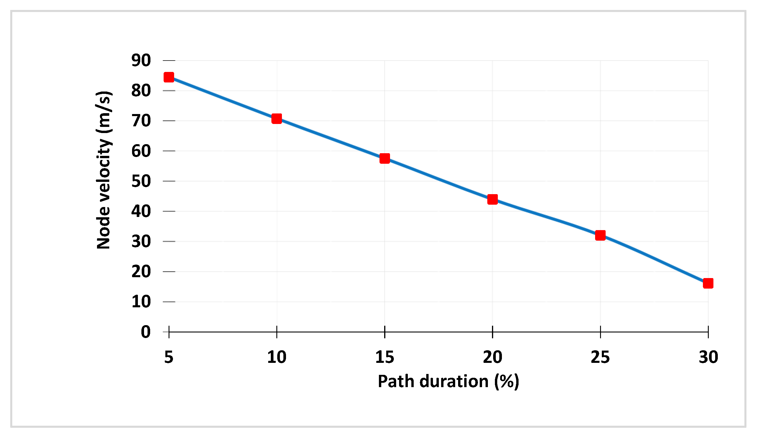
Figure 10 shows the relationship between the utilization ratio of the path duration and the velocity of the node.
From
Figure 10, it is assumed that the periodic update time is 15 s, which is the default value used by the NS3 simulation environment. It is observed that the utilization rate of the DSDV path duration decreases as the velocity of the nodes increases. This is because the path duration decreases with the increase in nodes’ velocity, while the periodic update remains constant.
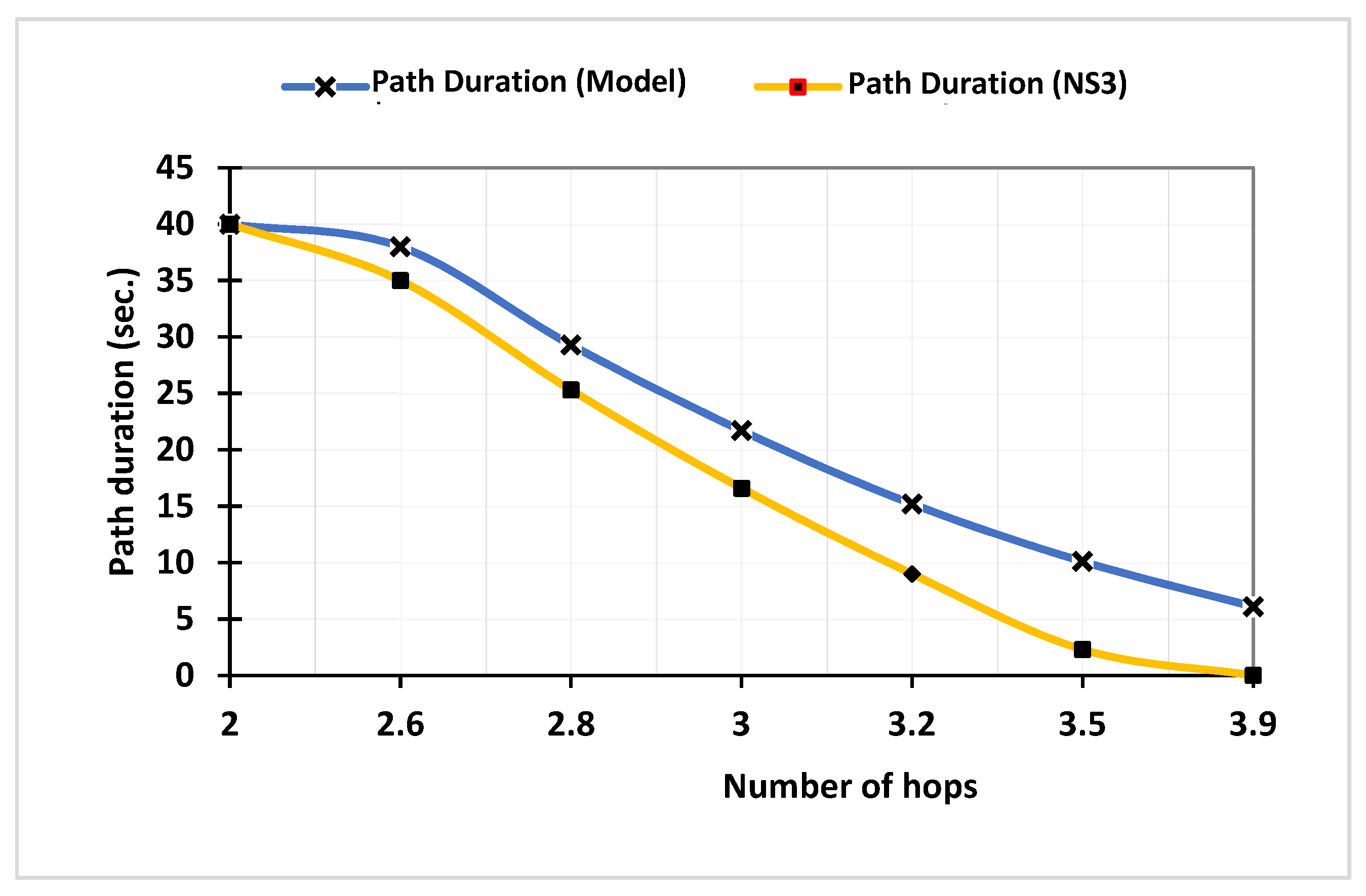
Figure 11 illustrates the relationship between the number of hops and the path duration. It is shown that the path duration is inversely proportional to the hop count, and it is considerably decreased when the hop count is greater 4. It is also noted that the actual path duration (Model) is greater than the observed DSDV path duration (NS3), and this difference increases with increasing the hop count metric. Furthermore, the path duration decreases more than the calculated path duration when the number of hops increases, and this can be attributed to the increase in the amount of data that must be exchanged by the nodes to update their records.
Furthermore, the path duration of the DSDV protocol decreases much faster than the actual path duration, as the duration of the delay is increased with the increase in the number of hops between the source and the destination. If it is assumed that the number of hops between the source and the destination equals 1, and that each node will wait 5 s before rebroadcasting its routing information, the DSDV path duration will be decreased by 5 s. On the other side, when the hop count between the source and the destination equals 2, the observed path duration will lose an additional 10 s compared to the actual path duration.
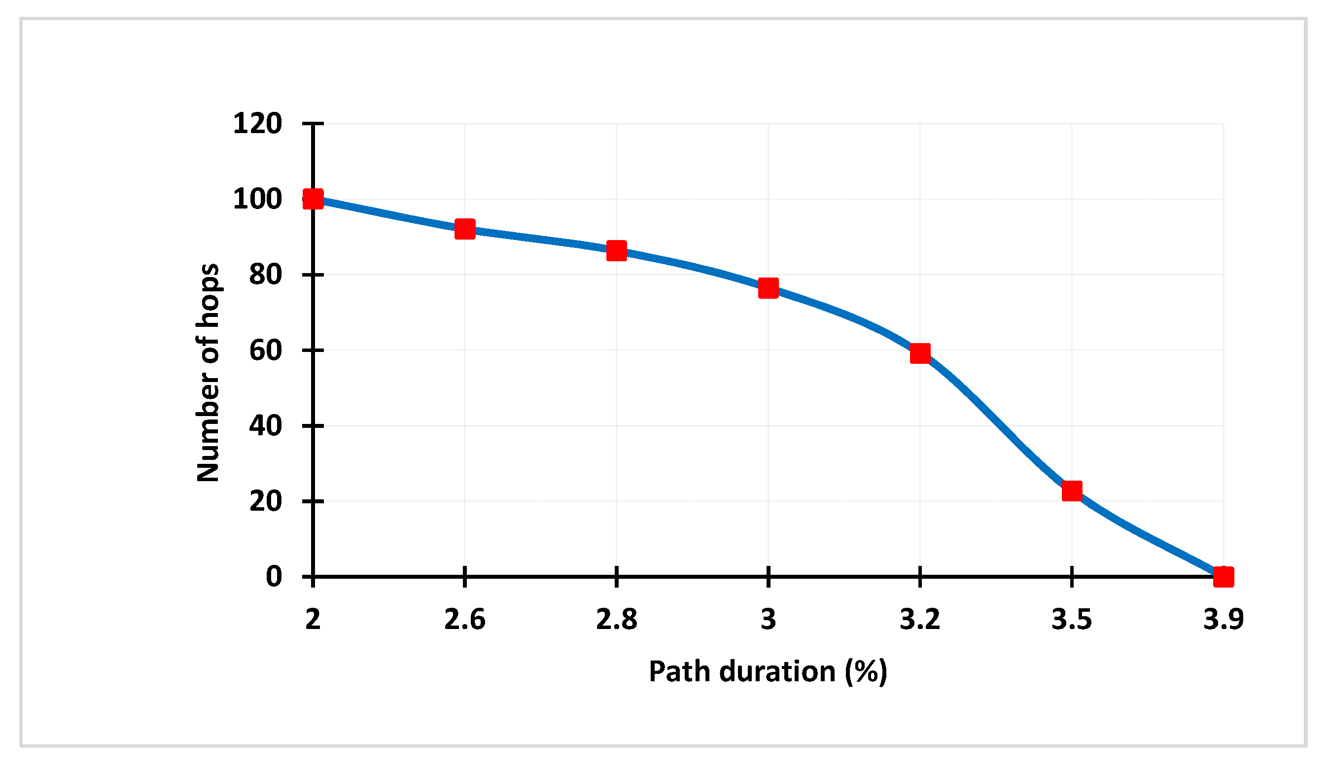
Finally,
Figure 12 shows the relationship between the number of hops and the path duration. It shows that the path duration is decreased when the number of hops becomes larger. It is also noted that the length of the path duration decreases significantly when the number of hops increases.
Table 2 summarizes the main findings of this research work. The results derived from the mathematical model are compared with those obtained from the simulation software. It is clearly shown that the path duration can be predicted analytically. When the node velocity changes from 5 to 30 m/s, the path duration is peaked at the beginning, and gradually decreases as velocity increases in an exponential distribution graph. The value-by-value comparison shows that the calculated values are aligned with the simulation values with an average of 5.6 m/s. This same analysis is valid for the number of hops. As this number increases, the path duration decreases. Normally, this situation could happen due to the process of finding the shortest path in routing protocols. The routing process works on minimizing the number of hops needed to reach the final destination by picking up longer links. These findings clearly indicate that the proposed mathematical model can give a good estimation of the link and path durations of the DSDV protocol.
5. Conclusions and Future Work
Routing in multi-hop ad hoc networks is a challenging task. Thus, analyzing routing protocols is essential to maintaining their development, modernization and maintenance. Various methods have been proposed to analyze routing protocols and evaluate their performance in a variety of scenarios. The majority of these methods used simulation testbeds; only very few contributions applied mathematical modeling to analyze reactive routing protocols. In this study, we have proposed a mathematical-based model targeting the DSDV protocol; it is one of the main widely deployed proactive routing protocols, with many new extensions and variants.
We tested the validity of the proposed model using simulations, and the results have shown that the DSDV path duration is inversely proportional to the speed of nodes, especially when this value exceeds 10 m/s. The path duration has the same curve, with better results due to the implementation of the settling time concept. Furthermore, we conclude that the rate of path utilization decreases with the increase of nodes’ speed, as it decreases in the path duration as the speed increases, and the periodic update interval remains constant. The path duration was significantly decreased when the number of hops becomes larger (more than three hops), even if the node’s speed was low. Furthermore, it has been shown that the settling time and keeping the periodic update interval fixed have a significant impact on the path duration and the path utilization rate. We have noticed that the protocol has a negative effect on the path duration when the number of hops increases—in contrast to the increase of the nodes’ speed, this effect remains limited.
As a future work, we will analyze both factors and try to reduce their impact without affecting other performance factors, such as routing overhead. Another research line is to study link duration, path duration and path utilization of routing protocols using other mobility models.


