Plant Disease Detection and Classification by Deep Learning


Abstract
:1. Introduction
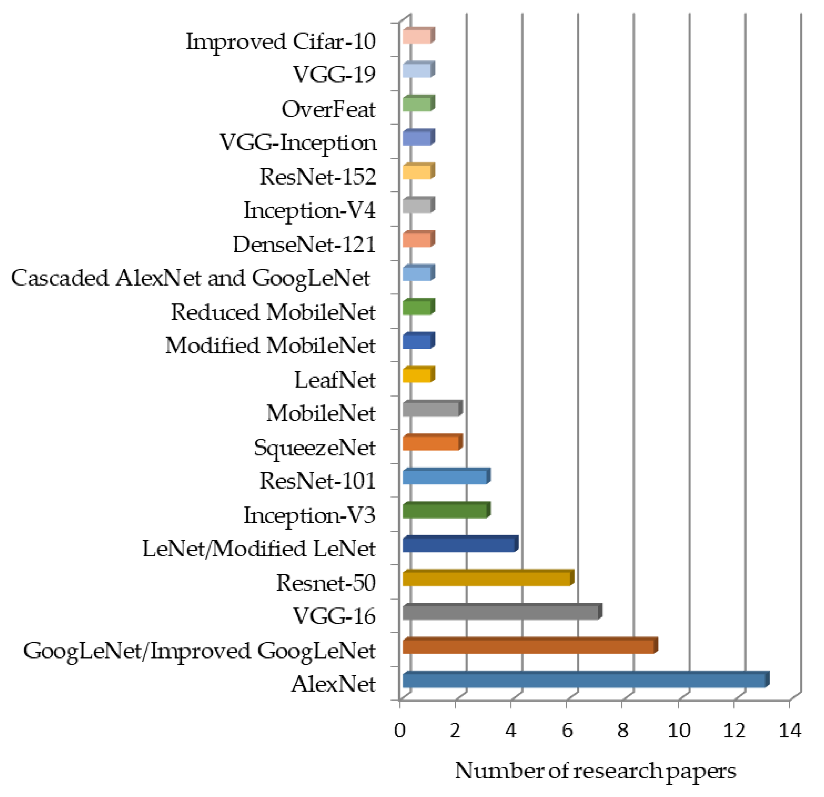
2. Plant Disease Detection by Well-Known DL Architectures
2.1. Implementation of DL Models
2.1.1. Without Visualization Technique
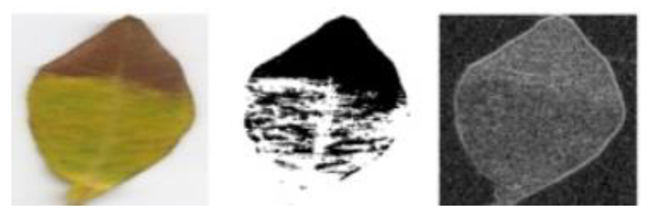
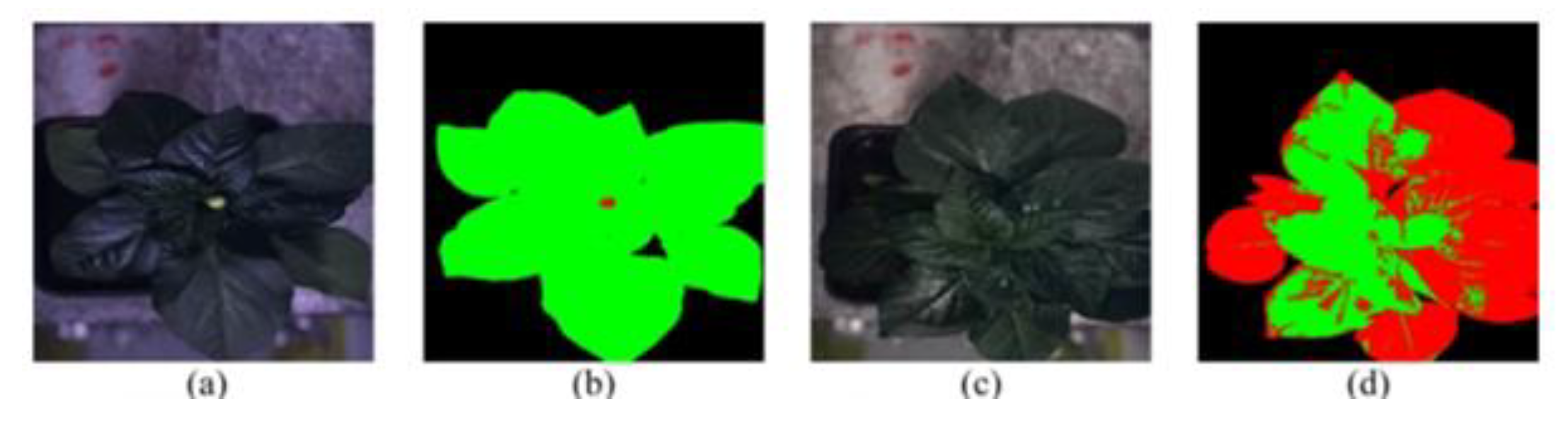
2.1.2. With Visualization Techniques
2.2. New/Modified DL Architectures for Plant-Disease Detection
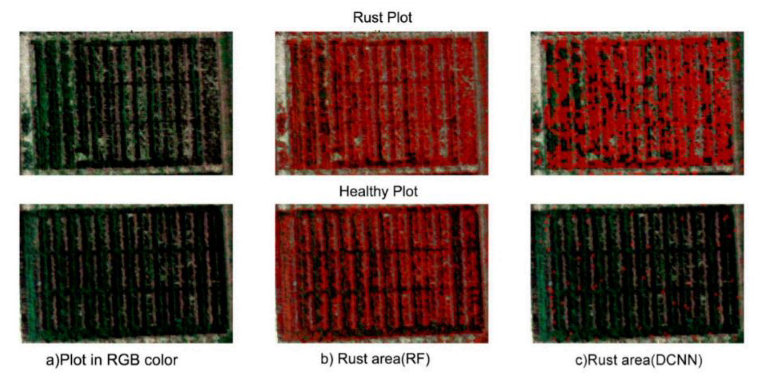
3. Hyper-Spectral Imaging with DL Models
4. Conclusions and Future Directions
- In most of the researches (as described in the previous sections), the PlantVillage dataset was used to evaluate the accuracy and performance of the respective DL models/architectures. Although this dataset has a lot of images of several plant species with their diseases, it has a simple/plain background. However, for a practical scenario, the real environment should be considered.
- Hyperspectral/multispectral imaging is an emerging technology and has been used in many areas of research (as described in Section 3). Therefore, it should be used with the efficient DL architectures to detect the plants’ diseases even before their symptoms are clearly apparent.
- A more efficient way of visualizing the spots of disease in plants should be introduced as it will save costs by avoiding the unnecessary application of fungicide/pesticide/herbicide.
- The severity of plant diseases changes with the passage of time, therefore, DL models should be improved/modified to enable them to detect and classify diseases during their complete cycle of occurrence.
- DL model/architecture should be efficient for many illumination conditions, so the datasets should not only indicate the real environment but also contain images taken in different field scenarios.
- A comprehensive study is required to understand the factors affecting the detection of plant diseases, like the classes and size of datasets, learning rate, illumination, and the like.
Author Contributions
Funding
Conflicts of Interest
Abbreviations
| ML | Machine Learning |
| DL | Deep Learning |
| CNN | Convolutional Neural network |
| DCNN | Deep Convolutional Neural Network |
| ILSVRC | ImageNet Large Scale Visual Recognition Challenge |
| RF | Random Forest |
| CA | Classification Accuracy |
| LSTM | Long Short-Term Memory |
| IoU | Intersection of Union |
| NiN | Network in Network |
| RCN | Region based Convolutional Neural Network |
| FCN | Fully Convolutional Neural Network |
| YOLO | You Only Look Once |
| SSD | Single Shot Detector |
| PSPNet | Pyramid Scene Parsing Network |
| IRRCNN | Inception Recurrent Residual Convolutional Neural Network |
| IRCNN | Inception Recurrent Convolutional Neural Network |
| DCRN | Densely Connected Recurrent Convolutional Network |
| INAR-SSD | Single Shot Detector with Inception module and Rainbow concatenation |
| R2U-Net | Recurrent Residual Convolutional Neural Network based on U-Net model |
| SVM | Support Vector Machines |
| ELM | Extreme Learning Machine |
| KNN | K-Nearest Neighbor |
| SRCNN | Super-Resolution Convolutional Neural Network |
| R-FCN | Region-based Fully Convolutional Networks |
| ROC | Receiver Operating Characteristic |
| PCA | Principal Component Analysis |
| MLP | Multi-Layer Perceptron |
| LRP | Layer-wise Relevance Propagation |
| HSI | Hyperspectral Imaging |
| FRKNN | Feature Ranking K-Nearest Neighbor |
| RNN | Recurrent Neural Network |
| ToF | Time-of-Flight |
| LR | Logistic Regression |
| GRU | Gated Recurrent Unit |
| AN | Generative Adversarial Nets |
| GPDCNN | Global Pooling Dilated Convolutional Neural Network |
| 2D-CNN-BidGRU | 2D-Convolutional-Bidirectional Gated Recurrent Unit Neural Network |
| OR-AC-GAN | Outlier Removal-Auxiliary Classifier-Generative Adversarial Nets |
References
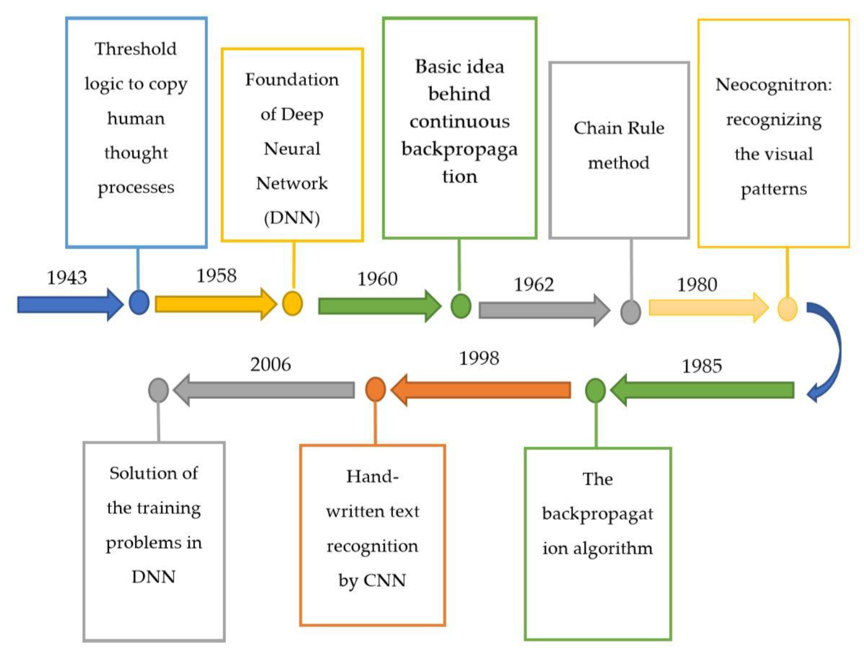
- McCulloch, W.S.; Pitts, W. A logical calculus of the ideas immanent in nervous activity. Bull. Math. Biophys. 1943, 5, 115–133. [Google Scholar] [CrossRef]
- Ackley, D.H.; Hinton, G.E.; Sejnowski, T.J. A learning algorithm for Boltzmann machines. Cogn. Sci. 1985, 9, 147–169. [Google Scholar] [CrossRef]
- Kelley, H.J. Gradient theory of optimal flight paths. Ars J. 1960, 30, 947–954. [Google Scholar] [CrossRef]
- Dreyfus, S. The numerical solution of variational problems. J. Math. Anal. Appl. 1962, 5, 30–45. [Google Scholar] [CrossRef] [Green Version]
- Fukushima, K. Neocognitron: A self-organizing neural network model for a mechanism of pattern recognition unaffected by shift in position. Biol. Cybern. 1980, 36, 193–202. [Google Scholar] [CrossRef]
- LeCun, Y.; Bottou, L.; Bengio, Y.; Haffner, P. Gradient-based learning applied to document recognition. Proc. IEEE 1998, 86, 2278–2324. [Google Scholar] [CrossRef] [Green Version]
- Hinton, G.E.; Osindero, S.; Teh, Y.-W. A fast learning algorithm for deep belief nets. Neural Comput. 2006, 18, 1527–1554. [Google Scholar] [CrossRef]
- Hinton, G.E.; Salakhutdinov, R.R. Reducing the dimensionality of data with neural networks. Science 2006, 313, 504–507. [Google Scholar] [CrossRef]
- Fayjie, A.R.; Hossain, S.; Oualid, D.; Lee, D.-J. Driverless Car: Autonomous Driving Using Deep Reinforcement Learning in Urban Environment. In Proceedings of the 2018 15th International Conference on Ubiquitous Robots (UR), Hawaii Convention Center, Honolulu, HI, USA, 26–30 June 2018; pp. 896–901. [Google Scholar]
- Hossain, S.; Lee, D.-J. Autonomous-Driving Vehicle Learning Environments using Unity Real-time Engine and End-to-End CNN Approach. J. Korea Robot. Soc. 2019, 14, 122–130. [Google Scholar] [CrossRef]
- Kocić, J.; Jovičić, N.; Drndarević, V. An End-to-End Deep Neural Network for Autonomous Driving Designed for Embedded Automotive Platforms. Sensors 2019, 19, 2064. [Google Scholar] [CrossRef]
- Esteva, A.; Robicquet, A.; Ramsundar, B.; Kuleshov, V.; DePristo, M.; Chou, K.; Cui, C.; Corrado, G.; Thrun, S.; Dean, J. A guide to deep learning in healthcare. Nat. Med. 2019, 25, 24. [Google Scholar] [CrossRef] [PubMed]
- Miotto, R.; Wang, F.; Wang, S.; Jiang, X.; Dudley, J.T. Deep learning for healthcare: Review, opportunities and challenges. Brief. Bioinform. 2017, 19, 1236–1246. [Google Scholar] [CrossRef] [PubMed]
- Ravì, D.; Wong, C.; Deligianni, F.; Berthelot, M.; Andreu-Perez, J.; Lo, B.; Yang, G.-Z. Deep learning for health informatics. IEEE J. Biomed. Health Inform. 2016, 21, 4–21. [Google Scholar] [CrossRef] [PubMed]
- Goodfellow, I.J.; Bulatov, Y.; Ibarz, J.; Arnoud, S.; Shet, V. Multi-digit number recognition from street view imagery using deep convolutional neural networks. arXiv 2013, arXiv:1312.6082. [Google Scholar]
- Jaderberg, M.; Simonyan, K.; Vedaldi, A.; Zisserman, A. Deep structured output learning for unconstrained text recognition. arXiv 2014, arXiv:1412.5903. [Google Scholar]
- Yousfi, S.; Berrani, S.-A.; Garcia, C. Deep learning and recurrent connectionist-based approaches for Arabic text recognition in videos. In Proceedings of the 2015 13th International Conference on Document Analysis and Recognition (ICDAR), Tunis, Tunisia, 23–26 August 2015; pp. 1026–1030. [Google Scholar]
- DeVries, P.M.; Viégas, F.; Wattenberg, M.; Meade, B.J. Deep learning of aftershock patterns following large earthquakes. Nature 2018, 560, 632. [Google Scholar] [CrossRef]
- Mousavi, S.M.; Zhu, W.; Sheng, Y.; Beroza, G.C. CRED: A deep residual network of convolutional and recurrent units for earthquake signal detection. Sci. Rep. 2019, 9, 10267. [Google Scholar] [CrossRef]
- Perol, T.; Gharbi, M.; Denolle, M. Convolutional neural network for earthquake detection and location. Sci. Adv. 2018, 4, e1700578. [Google Scholar] [CrossRef] [Green Version]
- Siau, K.; Yang, Y. Impact of artificial intelligence, robotics, and machine learning on sales and marketing. In Proceedings of the Twelve Annual Midwest Association for Information Systems Conference (MWAIS 2017), Springfield, IL, USA, 18–19 May 2017; pp. 18–19. [Google Scholar]
- Heaton, J.; Polson, N.; Witte, J.H. Deep learning for finance: Deep portfolios. Appl. Stoch. Models Bus. Ind. 2017, 33, 3–12. [Google Scholar] [CrossRef]
- Heaton, J.; Polson, N.G.; Witte, J.H. Deep learning in finance. arXiv 2016, arXiv:1602.06561. [Google Scholar]
- He, K.; Zhang, X.; Ren, S.; Sun, J. Deep residual learning for image recognition. In Proceedings of the IEEE Conference on Computer Vision and Pattern Recognition, Las Vegas, NV, USA, 26 June–1 July 2016; pp. 770–778. [Google Scholar]
- Mohanty, S.P.; Hughes, D.P.; Salathé, M. Using deep learning for image-based plant disease detection. Front. Plant Sci. 2016, 7, 1419. [Google Scholar] [CrossRef]
- Simonyan, K.; Zisserman, A. Very deep convolutional networks for large-scale image recognition. arXiv 2014, arXiv:1409.1556. [Google Scholar]
- Sladojevic, S.; Arsenovic, M.; Anderla, A.; Culibrk, D.; Stefanovic, D. Deep neural networks based recognition of plant diseases by leaf image classification. Comput. Intell. Neurosci. 2016, 2016. [Google Scholar] [CrossRef]
- Wan, J.; Wang, D.; Hoi, S.C.H.; Wu, P.; Zhu, J.; Zhang, Y.; Li, J. Deep learning for content-based image retrieval: A comprehensive study. In Proceedings of the 22nd ACM International Conference on Multimedia, Orlando, FL, USA, 3–7 November 2014; pp. 157–166. [Google Scholar]
- Wu, R.; Yan, S.; Shan, Y.; Dang, Q.; Sun, G. Deep image: Scaling up image recognition. arXiv 2015, arXiv:1501.02876. [Google Scholar]
- Krizhevsky, A.; Sutskever, I.; Hinton, G.E. Imagenet classification with deep convolutional neural networks. In Proceedings of the Advances in Neural Information Processing Systems, Lake Tahoe, NV, USA, 3–8 December 2012; pp. 1097–1105. [Google Scholar]
- Szegedy, C.; Liu, W.; Jia, Y.; Sermanet, P.; Reed, S.; Anguelov, D.; Erhan, D.; Vanhoucke, V.; Rabinovich, A. Going deeper with convolutions. In Proceedings of the IEEE Conference on Computer Vision and Pattern Recognition, Boston, MA, USA, 7–12 June 2015; pp. 1–9. [Google Scholar]
- Amara, J.; Bouaziz, B.; Algergawy, A. A Deep Learning-based Approach for Banana Leaf Diseases Classification. In Proceedings of the BTW (Workshops), Stuttgart, Germany, 6–10 March 2017; pp. 79–88. [Google Scholar]
- Rebetez, J.; Satizábal, H.F.; Mota, M.; Noll, D.; Büchi, L.; Wendling, M.; Cannelle, B.; Pérez-Uribe, A.; Burgos, S. Augmenting a convolutional neural network with local histograms—A case study in crop classification from high-resolution UAV imagery. In Proceedings of the ESANN, Bruges, Belgium, 27–29 April 2016. [Google Scholar]
- Rußwurm, M.; Körner, M. Multi-temporal land cover classification with long short-term memory neural networks. Int. Arch. Photogramm. Remote Sens. Spat. Inf. Sci. 2017, 42, 551. [Google Scholar] [CrossRef]
- TÜRKOĞLU, M.; Hanbay, D. Plant disease and pest detection using deep learning-based features. Turk. J. Electr. Eng. Comput. Sci. 2019, 27, 1636–1651. [Google Scholar] [CrossRef]
- Mortensen, A.K.; Dyrmann, M.; Karstoft, H.; Jørgensen, R.N.; Gislum, R. Semantic segmentation of mixed crops using deep convolutional neural network. In Proceedings of the CIGR-AgEng Conference, Aarhus, Denmark, 26–29 June 2016; Abstracts and Full Papers. pp. 1–6. [Google Scholar]
- Dyrmann, M.; Karstoft, H.; Midtiby, H.S. Plant species classification using deep convolutional neural network. Biosyst. Eng. 2016, 151, 72–80. [Google Scholar] [CrossRef]
- McCool, C.; Perez, T.; Upcroft, B. Mixtures of lightweight deep convolutional neural networks: Applied to agricultural robotics. IEEE Robot. Autom. Lett. 2017, 2, 1344–1351. [Google Scholar] [CrossRef]
- Santoni, M.M.; Sensuse, D.I.; Arymurthy, A.M.; Fanany, M.I. Cattle race classification using gray level co-occurrence matrix convolutional neural networks. Procedia Comput. Sci. 2015, 59, 493–502. [Google Scholar] [CrossRef]
- Sørensen, R.A.; Rasmussen, J.; Nielsen, J.; Jørgensen, R.N. Thistle detection using convolutional neural networks. In Proceedings of the 2017 EFITA WCCA CONGRESS, Montpellier, France, 2–6 July 2017; p. 161. [Google Scholar]
- Xinshao, W.; Cheng, C. Weed seeds classification based on PCANet deep learning baseline. In Proceedings of the 2015 Asia-Pacific Signal and Information Processing Association Annual Summit and Conference (APSIPA), Hong Kong, China, 16–19 December 2015; pp. 408–415. [Google Scholar]
- Hall, D.; McCool, C.; Dayoub, F.; Sunderhauf, N.; Upcroft, B. Evaluation of features for leaf classification in challenging conditions. In Proceedings of the 2015 IEEE Winter Conference on Applications of Computer Vision, Waikoloa Beach, HI, USA, 6–8 January 2015; pp. 797–804. [Google Scholar]
- Kamilaris, A.; Prenafeta-Boldú, F.X. Deep learning in agriculture: A survey. Comput. Electron. Agric. 2018, 147, 70–90. [Google Scholar] [CrossRef] [Green Version]
- Itzhaky, Y.; Farjon, G.; Khoroshevsky, F.; Shpigler, A.; Bar-Hillel, A. Leaf counting: Multiple scale regression and detection using deep CNNs. In Proceedings of the BMVC, North East, UK, 3–6 September 2018; p. 328. [Google Scholar]
- Ubbens, J.; Cieslak, M.; Prusinkiewicz, P.; Stavness, I. The use of plant models in deep learning: An application to leaf counting in rosette plants. Plant Methods 2018, 14, 6. [Google Scholar] [CrossRef]
- Rahnemoonfar, M.; Sheppard, C. Deep count: Fruit counting based on deep simulated learning. Sensors 2017, 17, 905. [Google Scholar] [CrossRef]
- Kussul, N.; Lavreniuk, M.; Skakun, S.; Shelestov, A. Deep learning classification of land cover and crop types using remote sensing data. IEEE Geosci. Remote Sens. Lett. 2017, 14, 778–782. [Google Scholar] [CrossRef]
- Grinblat, G.L.; Uzal, L.C.; Larese, M.G.; Granitto, P.M. Deep learning for plant identification using vein morphological patterns. Comput. Electron. Agric. 2016, 127, 418–424. [Google Scholar] [CrossRef]
- Lee, S.H.; Chan, C.S.; Wilkin, P.; Remagnino, P. Deep-plant: Plant identification with convolutional neural networks. In Proceedings of the 2015 IEEE International Conference on Image Processing (ICIP), Québec City, QC, Canada, 27–30 September 2015; pp. 452–456. [Google Scholar]
- Pound, M.P.; Atkinson, J.A.; Townsend, A.J.; Wilson, M.H.; Griffiths, M.; Jackson, A.S.; Bulat, A.; Tzimiropoulos, G.; Wells, D.M.; Murchie, E.H. Deep machine learning provides state-of-the-art performance in image-based plant phenotyping. Gigascience 2017, 6, gix083. [Google Scholar] [CrossRef] [PubMed]
- Milioto, A.; Lottes, P.; Stachniss, C. Real-time blob-wise sugar beets vs weeds classification for monitoring fields using convolutional neural networks. Isprs Ann. Photogramm. Remote Sens. Spat. Inf. Sci. 2017, 4, 41. [Google Scholar] [CrossRef]
- Potena, C.; Nardi, D.; Pretto, A. Fast and accurate crop and weed identification with summarized train sets for precision agriculture. In Proceedings of the International Conference on Intelligent Autonomous Systems, Shanghai, China, 3–7 July 2016; pp. 105–121. [Google Scholar]
- Sun, Y.; Liu, Y.; Wang, G.; Zhang, H. Deep learning for plant identification in natural environment. Comput. Intell. Neurosci. 2017, 2017, 7361042. [Google Scholar] [CrossRef] [PubMed]
- Singh, A.K.; Ganapathysubramanian, B.; Sarkar, S.; Singh, A. Deep learning for plant stress phenotyping: Trends and future perspectives. Trends Plant Sci. 2018, 23, 883–898. [Google Scholar] [CrossRef] [PubMed]
- Brahimi, M.; Arsenovic, M.; Laraba, S.; Sladojevic, S.; Boukhalfa, K.; Moussaoui, A. Deep learning for plant diseases: Detection and saliency map visualisation. In Human and Machine Learning; Springer: Berlin, Germany, 2018; pp. 93–117. [Google Scholar]
- Sibiya, M.; Sumbwanyambe, M. A Computational Procedure for the Recognition and Classification of Maize Leaf Diseases Out of Healthy Leaves Using Convolutional Neural Networks. AgriEngineering 2019, 1, 119–131. [Google Scholar] [CrossRef] [Green Version]
- Zhang, K.; Wu, Q.; Liu, A.; Meng, X. Can Deep Learning Identify Tomato Leaf Disease? Adv. Multimed. 2018, 2018, 10. [Google Scholar] [CrossRef]
- Ferentinos, K.P. Deep learning models for plant disease detection and diagnosis. Comput. Electron. Agric. 2018, 145, 311–318. [Google Scholar] [CrossRef]
- Ramcharan, A.; Baranowski, K.; McCloskey, P.; Ahmed, B.; Legg, J.; Hughes, D.P. Deep learning for image-based cassava disease detection. Front. Plant Sci. 2017, 8, 1852. [Google Scholar] [CrossRef]
- Fujita, E.; Kawasaki, Y.; Uga, H.; Kagiwada, S.; Iyatomi, H. Basic investigation on a robust and practical plant diagnostic system. In Proceedings of the 2016 15th IEEE International Conference on Machine Learning and Applications (ICMLA), Anaheim, CA, USA, 18–20 December 2016; pp. 989–992. [Google Scholar]
- Yamamoto, K.; Togami, T.; Yamaguchi, N. Super-resolution of plant disease images for the acceleration of image-based phenotyping and vigor diagnosis in agriculture. Sensors 2017, 17, 2557. [Google Scholar] [CrossRef]
- Durmuş, H.; Güneş, E.O.; Kırcı, M. Disease detection on the leaves of the tomato plants by using deep learning. In Proceedings of the 2017 6th International Conference on Agro-Geoinformatics, Fairfax, VA, USA, 7–10 August 2017; pp. 1–5. [Google Scholar]
- Too, E.C.; Yujian, L.; Njuki, S.; Yingchun, L. A comparative study of fine-tuning deep learning models for plant disease identification. Comput. Electron. Agric. 2019, 161, 272–279. [Google Scholar] [CrossRef]
- Rangarajan, A.K.; Purushothaman, R.; Ramesh, A. Tomato crop disease classification using pre-trained deep learning algorithm. Procedia Comput. Sci. 2018, 133, 1040–1047. [Google Scholar] [CrossRef]
- Cruz, A.C.; Luvisi, A.; De Bellis, L.; Ampatzidis, Y. Vision-based plant disease detection system using transfer and deep learning. In Proceedings of the 2017 ASABE Annual International Meeting, Spokane, WA, USA, 16–19 July 2017; p. 1. [Google Scholar]
- Ma, J.; Du, K.; Zheng, F.; Zhang, L.; Gong, Z.; Sun, Z. A recognition method for cucumber diseases using leaf symptom images based on deep convolutional neural network. Comput. Electron. Agric. 2018, 154, 18–24. [Google Scholar] [CrossRef]
- Brahimi, M.; Mahmoudi, S.; Boukhalfa, K.; Moussaoui, A. Deep interpretable architecture for plant diseases classification. arXiv 2019, arXiv:1905.13523. [Google Scholar] [Green Version]
- Fuentes, A.; Yoon, S.; Kim, S.; Park, D. A robust deep-learning-based detector for real-time tomato plant diseases and pests recognition. Sensors 2017, 17, 2022. [Google Scholar] [CrossRef] [PubMed]
- Selvaraj, M.G.; Vergara, A.; Ruiz, H.; Safari, N.; Elayabalan, S.; Ocimati, W.; Blomme, G. AI-powered banana diseases and pest detection. Plant Methods 2019, 15, 92. [Google Scholar] [CrossRef]
- DeChant, C.; Wiesner-Hanks, T.; Chen, S.; Stewart, E.L.; Yosinski, J.; Gore, M.A.; Nelson, R.J.; Lipson, H. Automated identification of northern leaf blight-infected maize plants from field imagery using deep learning. Phytopathology 2017, 107, 1426–1432. [Google Scholar] [CrossRef]
- Wallelign, S.; Polceanu, M.; Buche, C. Soybean Plant Disease Identification Using Convolutional Neural Network. In Proceedings of the Thirty-First International Flairs Conference, Melbourne, FL, USA, 21–23 May 2018. [Google Scholar]
- Brahimi, M.; Boukhalfa, K.; Moussaoui, A. Deep learning for tomato diseases: Classification and symptoms visualization. Appl. Artif. Intell. 2017, 31, 299–315. [Google Scholar] [CrossRef]
- Lu, J.; Hu, J.; Zhao, G.; Mei, F.; Zhang, C. An in-field automatic wheat disease diagnosis system. Comput. Electron. Agric. 2017, 142, 369–379. [Google Scholar] [CrossRef] [Green Version]
- Ha, J.G.; Moon, H.; Kwak, J.T.; Hassan, S.I.; Dang, M.; Lee, O.N.; Park, H.Y. Deep convolutional neural network for classifying Fusarium wilt of radish from unmanned aerial vehicles. J. Appl. Remote Sens. 2017, 11, 042621. [Google Scholar] [CrossRef]
- Lin, K.; Gong, L.; Huang, Y.; Liu, C.; Pan, J. Deep learning-based segmentation and quantification of cucumber Powdery Mildew using convolutional neural network. Front. Plant Sci. 2019, 10, 155. [Google Scholar] [CrossRef]
- Barbedo, J.G.A. Plant disease identification from individual lesions and spots using deep learning. Biosyst. Eng. 2019, 180, 96–107. [Google Scholar] [CrossRef]
- Ghosal, S.; Blystone, D.; Singh, A.K.; Ganapathysubramanian, B.; Singh, A.; Sarkar, S. An explainable deep machine vision framework for plant stress phenotyping. Proc. Natl. Acad. Sci. 2018, 115, 4613–4618. [Google Scholar] [CrossRef] [PubMed] [Green Version]
- Lu, Y.; Yi, S.; Zeng, N.; Liu, Y.; Zhang, Y. Identification of rice diseases using deep convolutional neural networks. Neurocomputing 2017, 267, 378–384. [Google Scholar] [CrossRef]
- Picon, A.; Alvarez-Gila, A.; Seitz, M.; Ortiz-Barredo, A.; Echazarra, J.; Johannes, A. Deep convolutional neural networks for mobile capture device-based crop disease classification in the wild. Comput. Electron. Agric. 2019, 161, 280–290. [Google Scholar] [CrossRef]
- Johannes, A.; Picon, A.; Alvarez-Gila, A.; Echazarra, J.; Rodriguez-Vaamonde, S.; Navajas, A.D.; Ortiz-Barredo, A. Automatic plant disease diagnosis using mobile capture devices, applied on a wheat use case. Comput. Electron. Agric. 2017, 138, 200–209. [Google Scholar] [CrossRef]
- Zhang, S.; Zhang, S.; Zhang, C.; Wang, X.; Shi, Y. Cucumber leaf disease identification with global pooling dilated convolutional neural network. Comput. Electron. Agric. 2019, 162, 422–430. [Google Scholar] [CrossRef]
- Khan, M.A.; Akram, T.; Sharif, M.; Awais, M.; Javed, K.; Ali, H.; Saba, T. CCDF: Automatic system for segmentation and recognition of fruit crops diseases based on correlation coefficient and deep CNN features. Comput. Electron. Agric. 2018, 155, 220–236. [Google Scholar] [CrossRef]
- Kerkech, M.; Hafiane, A.; Canals, R. Deep leaning approach with colorimetric spaces and vegetation indices for vine diseases detection in UAV images. Comput. Electron. Agric. 2018, 155, 237–243. [Google Scholar] [CrossRef]
- Nagasubramanian, K.; Jones, S.; Singh, A.K.; Singh, A.; Ganapathysubramanian, B.; Sarkar, S. Explaining hyperspectral imaging based plant disease identification: 3D CNN and saliency maps. arXiv 2018, arXiv:1804.08831. [Google Scholar]
- Jiang, P.; Chen, Y.; Liu, B.; He, D.; Liang, C. Real-Time Detection of Apple Leaf Diseases Using Deep Learning Approach Based on Improved Convolutional Neural Networks. IEEE Access 2019, 7, 59069–59080. [Google Scholar] [CrossRef]
- Zhang, X.; Qiao, Y.; Meng, F.; Fan, C.; Zhang, M. Identification of maize leaf diseases using improved deep convolutional neural networks. IEEE Access 2018, 6, 30370–30377. [Google Scholar] [CrossRef]
- Liu, B.; Zhang, Y.; He, D.; Li, Y. Identification of apple leaf diseases based on deep convolutional neural networks. Symmetry 2017, 10, 11. [Google Scholar] [CrossRef]
- Chen, J.; Liu, Q.; Gao, L. Visual Tea Leaf Disease Recognition Using a Convolutional Neural Network Model. Symmetry 2019, 11, 343. [Google Scholar] [CrossRef]
- Kamal, K.; Yin, Z.; Wu, M.; Wu, Z. Depthwise separable convolution architectures for plant disease classification. Comput. Electron. Agric. 2019, 165, 104948. [Google Scholar]
- Arsenovic, M.; Karanovic, M.; Sladojevic, S.; Anderla, A.; Stefanovic, D. Solving Current Limitations of Deep Learning Based Approaches for Plant Disease Detection. Symmetry 2019, 11, 939. [Google Scholar] [CrossRef]
- Veys, C.; Chatziavgerinos, F.; AlSuwaidi, A.; Hibbert, J.; Hansen, M.; Bernotas, G.; Smith, M.; Yin, H.; Rolfe, S.; Grieve, B. Multispectral imaging for presymptomatic analysis of light leaf spot in oilseed rape. Plant Methods 2019, 15, 4. [Google Scholar] [CrossRef] [PubMed]
- Mahlein, A.-K.; Alisaac, E.; Al Masri, A.; Behmann, J.; Dehne, H.-W.; Oerke, E.-C. Comparison and Combination of Thermal, Fluorescence, and Hyperspectral Imaging for Monitoring Fusarium Head Blight of Wheat on Spikelet Scale. Sensors 2019, 19, 2281. [Google Scholar] [CrossRef] [PubMed]
- Xie, C.; Yang, C.; He, Y. Hyperspectral imaging for classification of healthy and gray mold diseased tomato leaves with different infection severities. Comput. Electron. Agric. 2017, 135, 154–162. [Google Scholar] [CrossRef]
- Shuaibu, M.; Lee, W.S.; Schueller, J.; Gader, P.; Hong, Y.K.; Kim, S. Unsupervised hyperspectral band selection for apple Marssonina blotch detection. Comput. Electron. Agric. 2018, 148, 45–53. [Google Scholar] [CrossRef]
- Chen, T.; Zhang, J.; Chen, Y.; Wan, S.; Zhang, L. Detection of peanut leaf spots disease using canopy hyperspectral reflectance. Comput. Electron. Agric. 2019, 156, 677–683. [Google Scholar] [CrossRef]
- Moghadam, P.; Ward, D.; Goan, E.; Jayawardena, S.; Sikka, P.; Hernandez, E. Plant disease detection using hyperspectral imaging. In Proceedings of the 2017 International Conference on Digital Image Computing: Techniques and Applications (DICTA), Sydney, Australia, 29 November–1 December 2017; pp. 1–8. [Google Scholar]
- Hruška, J.; Adão, T.; Pádua, L.; Marques, P.; Cunha, A.; Peres, E.; Sousa, A.; Morais, R.; Sousa, J.J. Machine learning classification methods in hyperspectral data processing for agricultural applications. In Proceedings of the International Conference on Geoinformatics and Data Analysis, Prague, Czech Republic, 20–22 April 2018; pp. 137–141. [Google Scholar]
- Ashourloo, D.; Aghighi, H.; Matkan, A.A.; Mobasheri, M.R.; Rad, A.M. An investigation into machine learning regression techniques for the leaf rust disease detection using hyperspectral measurement. IEEE J. Sel. Top. Appl. Earth Obs. Remote Sens. 2016, 9, 4344–4351. [Google Scholar] [CrossRef]
- Su, J.; Liu, C.; Coombes, M.; Hu, X.; Wang, C.; Xu, X.; Li, Q.; Guo, L.; Chen, W.-H. Wheat yellow rust monitoring by learning from multispectral UAV aerial imagery. Comput. Electron. Agric. 2018, 155, 157–166. [Google Scholar] [CrossRef]
- Rumpf, T.; Mahlein, A.-K.; Steiner, U.; Oerke, E.-C.; Dehne, H.-W.; Plümer, L. Early detection and classification of plant diseases with support vector machines based on hyperspectral reflectance. Comput. Electron. Agric. 2010, 74, 91–99. [Google Scholar] [CrossRef]
- Zhu, H.; Chu, B.; Zhang, C.; Liu, F.; Jiang, L.; He, Y. Hyperspectral imaging for presymptomatic detection of tobacco disease with successive projections algorithm and machine-learning classifiers. Sci. Rep. 2017, 7, 4125. [Google Scholar] [CrossRef] [PubMed]
- Halicek, M.; Lu, G.; Little, J.V.; Wang, X.; Patel, M.; Griffith, C.C.; El-Deiry, M.W.; Chen, A.Y.; Fei, B. Deep convolutional neural networks for classifying head and neck cancer using hyperspectral imaging. J. Biomed. Opt. 2017, 22, 060503. [Google Scholar] [CrossRef] [PubMed]
- Ma, X.; Geng, J.; Wang, H. Hyperspectral image classification via contextual deep learning. Eurasip J. Image Video Process. 2015, 2015, 20. [Google Scholar] [CrossRef] [Green Version]
- Paoletti, M.; Haut, J.; Plaza, J.; Plaza, A. A new deep convolutional neural network for fast hyperspectral image classification. Isprs J. Photogramm. Remote Sens. 2018, 145, 120–147. [Google Scholar] [CrossRef]
- Hu, W.; Huang, Y.; Wei, L.; Zhang, F.; Li, H. Deep convolutional neural networks for hyperspectral image classification. J. Sens. 2015, 2015. [Google Scholar] [CrossRef]
- Chen, Y.; Jiang, H.; Li, C.; Jia, X.; Ghamisi, P. Deep feature extraction and classification of hyperspectral images based on convolutional neural networks. IEEE Trans. Geosci. Remote Sens. 2016, 54, 6232–6251. [Google Scholar] [CrossRef]
- Mou, L.; Ghamisi, P.; Zhu, X.X. Deep recurrent neural networks for hyperspectral image classification. IEEE Trans. Geosci. Remote Sens. 2017, 55, 3639–3655. [Google Scholar] [CrossRef]
- Wu, H.; Prasad, S. Convolutional recurrent neural networks forhyperspectral data classification. Remote Sens. 2017, 9, 298. [Google Scholar] [CrossRef]
- Yue, J.; Zhao, W.; Mao, S.; Liu, H. Spectral–spatial classification of hyperspectral images using deep convolutional neural networks. Remote Sens. Lett. 2015, 6, 468–477. [Google Scholar] [CrossRef]
- Signoroni, A.; Savardi, M.; Baronio, A.; Benini, S. Deep Learning Meets Hyperspectral Image Analysis: A Multidisciplinary Review. J. Imaging 2019, 5, 52. [Google Scholar] [CrossRef]
- Jin, X.; Jie, L.; Wang, S.; Qi, H.; Li, S. Classifying wheat hyperspectral pixels of healthy heads and Fusarium head blight disease using a deep neural network in the wild field. Remote Sens. 2018, 10, 395. [Google Scholar] [CrossRef]
- Wang, D.; Vinson, R.; Holmes, M.; Seibel, G.; Bechar, A.; Nof, S.; Tao, Y. Early Detection of Tomato Spotted Wilt Virus by Hyperspectral Imaging and Outlier Removal Auxiliary Classifier Generative Adversarial Nets (OR-AC-GAN). Sci. Rep. 2019, 9, 4377. [Google Scholar] [CrossRef] [PubMed]
- Polder, G.; Blok, P.M.; de Villiers, H.A.C.; van der Wolf, J.M.; Kamp, J. Potato Virus Y Detection in Seed Potatoes Using Deep Learning on Hyperspectral Images. Front. Plant Sci. 2019, 10. [Google Scholar] [CrossRef] [PubMed]
- Zhang, X.; Han, L.; Dong, Y.; Shi, Y.; Huang, W.; Han, L.; González-Moreno, P.; Ma, H.; Ye, H.; Sobeih, T. A Deep Learning-Based Approach for Automated Yellow Rust Disease Detection from High-Resolution Hyperspectral UAV Images. Remote Sens. 2019, 11, 1554. [Google Scholar] [CrossRef]
- Golhani, K.; Balasundram, S.K.; Vadamalai, G.; Pradhan, B. A review of neural networks in plant disease detection using hyperspectral data. Inf. Process. Agric. 2018, 5, 354–371. [Google Scholar] [CrossRef]


| Deep Learning Models | Parameters | Key Features and Pros/Cons |
|---|---|---|
| LeNet | 60k | First CNN model. Few parameters as compared to other CNNmodels. Limited capability of computation |
| AlexNet | 60M | Known as the first modern CNN. Best image recognition performance at its time. Used ReLU to achieve better performance. Dropout technique was used to avoid overfitting |
| OverFeat | 145M | First model used for detection, localization, and classification of objects through a single CNN. Large number of parameters as compared to AlexNet |
| ZFNet | 42.6M | Reduced weights (as compared to AlexNet) by considering 7 × 7 kernels and improved accuracy |
| VGG | 133M–144M | 3 × 3 receptive fields were considered to include more number of non-linearity functions which made decision function discriminative. Computationally expensive model due to large number of parameters |
| GoogLeNet | 7M | Fewer number of parameters as compared to AlexNet model. Better accuracy at its time |
| ResNet | 25.5M | Vanishing gradient problem was addressed. Better accuracy than VGG and GoogLeNet models |
| DenseNet | 7.1M | Dense connections between the layers. Reduced number of parameters with better accuracy |
| SqueezeNet | 1.25M | Similar accuracy as AlexNet with 50 times lesser parameters. Considered 1 × 1 filters instead of 3 × 3 filters. Input channels were decreased. Large activation maps of convolution layers |
| Xception | 22.8M | A depth-wise separable convolution approach. Performed better than VGG, ResNet, and Inception-v3 models |
| MobileNet | 4.2M | Considered the depth-wise separable convolution concept. Reduced parameters significantly. Achieved accuracy near to VGG and GoogLeNet |
| Modified/Reduced MobileNet | 0.5/0.54M | Lesser number of parameters as compared to MobileNet. Similar accuracy as compared to MobileNet |
| VGG-Inception | 132M | A cascaded version of VGG and inception module. The number of parameters were reduced by substituting 5 × 5 convolution layers with two 3 × 3 layers. Testing accuracy was increased as compared to many well-known DL models like AlexNet, GoogLeNet, Inception-v3, ResNet, and VGG-16. |
| Visualization Techniques/Mappings | References |
|---|---|
| Visualization of features having filter from first to final layer | [27] |
| Visualize activations in first convolutional layer | [25] |
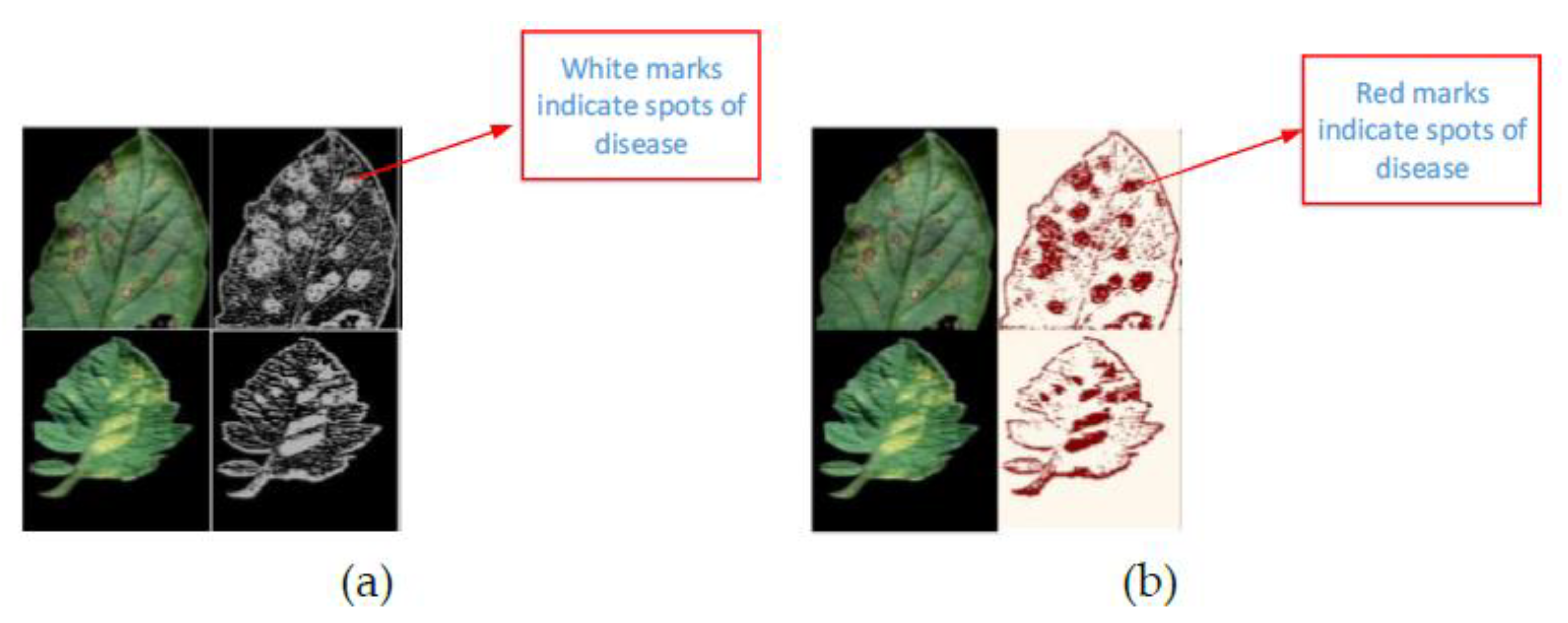
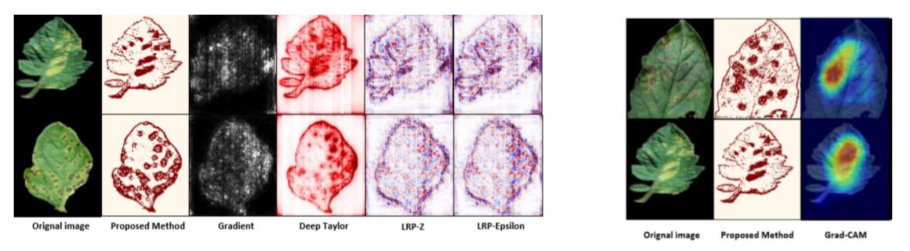
| Saliency map visualization | [55] |
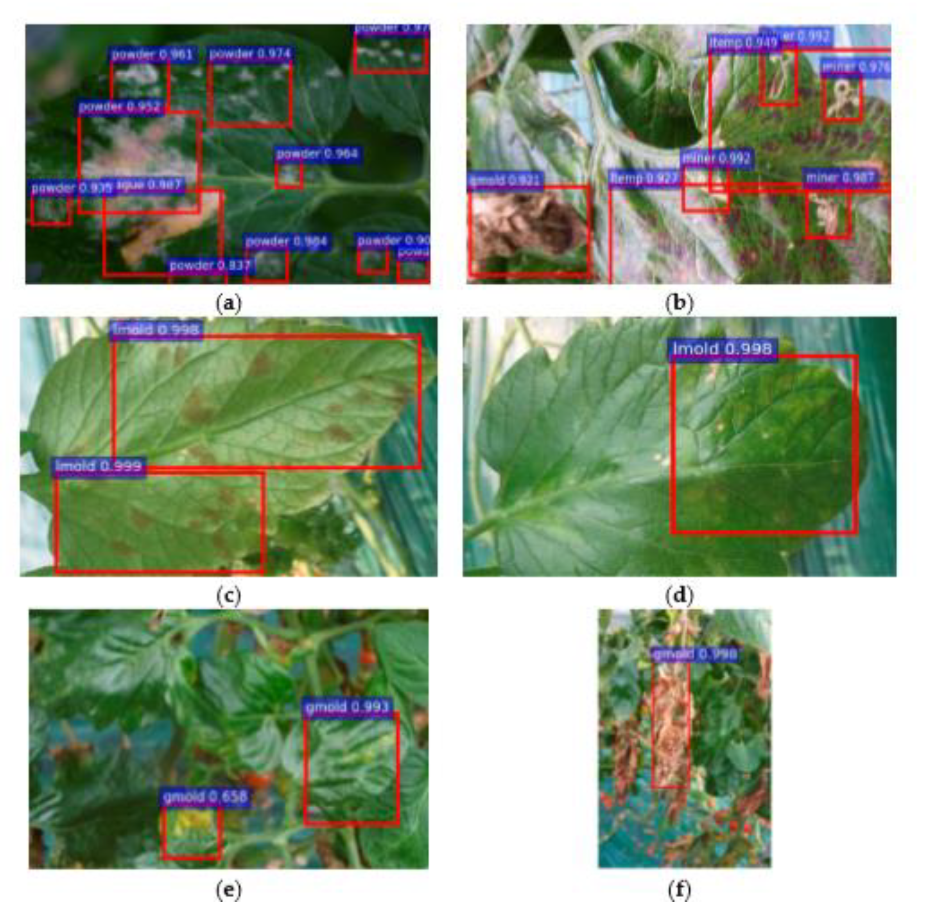
| Classification and localization of diseases by bounding boxes | [68] |
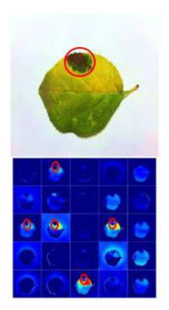
| Heat maps were used to identify the spots of the disease | [70] |
| Feature map for the diseased rice plant | [78] |
| Symptoms visualization method | [72] |
| Feature and spatial core maps | [73] |
| Color space into HSV and K-means clustering | [74] |
| Feature map for spotting the diseases | [77] |
| Image segmentation method | [66] |
| Reconstruction of images on discriminant regions, segmentation of images by binary threshold theorem, and heat map construction | [67] |
| Saliency map visualization | [84] |
| Saliency map, 2D and 3D contour, mesh graph image | [82] |
| Activation visualization | [85] |
| Segmentation map and edge map | [65] |
| DL Architectures/Algorithms | Datasets | Selected Plant/s | Performance Metrics (and Their Results) | Refs |
|---|---|---|---|---|
| CNN | PlantVillage | Maize | CA (92.85%) | [56] |
| AlexNet, GoogLeNet, ResNet | PlantVillage | Tomato | CA by ResNet which gave the best value (97.28%) | [57] |
| LeNet | PlantVillage | Banana | CA (98.61%), F1 (98.64%) | [32] |
| AlexNet, ALexNetOWTBn, GoogLeNet, Overfeat, VGG | PlantVillage and in-field images | Apple, blueberry, banana, cabbage, cassava, cantaloupe, celery, cherry, cucumber, corn, eggplant, gourd, grape, orange, onion | Success rate of VGG (99.53%) which is the best among all | [58] |
| AlexNet, VGG16, VGG 19, SqueezeNet, GoogLeNet, Inceptionv3, InceptionResNetv2, ResNet50, Resnet101 | Real field dataset | Apricot, Walnut, Peach, Cherry | F1(97.14), Accuracy (97.86 ± 1.56) of ResNet | [35] |
| Inceptionv3 | Experimental field dataset | Cassava | CA (93%) | [59] |
| CNN | Images taken from the research center | Cucumber | CA (82.3%) | [60] |
| Super-Resolution Convolutional Neural Network (SCRNN) | PlantVillage | Tomato | Accuracy (~90%) | [61] |
| CaffeNet | Downloaded from the internet | Pear, cherry, peach, apple, grapevine | Precision (96.3%) | [27] |
| AlexNet and GoogLeNet | PlantVillage | Apple, blueberry, bell pepper, cherry, corn, peach, grape, raspberry, potato, squash, soybean, strawberry, tomato | CA (99.35%) of GoogLeNet | [25] |
| AlexNet, GoogLeNet, VGG- 16, ResNet-50,101, ResNetXt-101, Faster RCNN, SSD, R-FCN, ZFNet | Image taken in real fields | Tomato | Precision (85.98%) of ResNet-50 with Region based Fully Convolutional Network(R-FCN) | [68] |
| CNN | Bisque platform of Cy Verse | Maize | Accuracy (96.7%) | [70] |
| DCNN | Images were taken in real field | Rice | Accuracy (95.48%) | [78] |
| AlexNet, GoogLeNet | PlantVillage | Tomato | Accuracy (0.9918 ± 0.169) of GoogLeNet | [72] |
| VGG-FCN-VD16 and VGG-FCN-S | Wheat Disease Database 2017 | Wheat | Accuracy (97.95%) of VGG-FCN-VD16 | [73] |
| VGG-A, CNN | Images were taken in real field | Radish | Accuracy (93.3%) | [74] |
| AlexNet | Images were taken in real field | Soybean | CA (94.13%) | [77] |
| AlexNet and SqueezeNet v1.1 | PlantVillage | Tomato | CA (95.65%) of AlexNet | [62] |
| DCNN, Random forest, Support Vector Machine and AlexNet | PlantVillage dataset, Forestry Image dataset and agricultural field in China | Cucumber | CA (93.4%) of DCNN | [66] |
| Teacher/student architecture | PlantVillage | Apple, bell pepper, blueberry, cherry, corn, orange, grape, potato, raspberry, peach, soybean, strawberry, tomato, squash | Training accuracy and loss (~99%,~0–0.5%), validation accuracy and loss (~95%, ~10%) | [67] |
| Improved GoogLeNet, Cifar-10 | PlantVillage and various websites | Maize | Top-1 accuracy (98.9%) of improved GoogLeNet | [86] |
| MobileNet, Modified MobileNet, Reduced MobileNet | PlantVillage dataset | 24 types of plant | CA (98.34%) of reduced MobileNet | [89] |
| VGG-16, ResNet-50,101,152, Inception-V4 and DenseNets-121 | PlantVillage | Apple, bell pepper, blueberry, cherry, corn, orange, grape, potato, raspberry, peach, soybean, strawberry, tomato, squash | Testing accuracy (99.75%) of DenseNets | [63] |
| User defined CNN, SVM, AlexNet, GoogLeNet, ResNet-20 and VGG-16 | Images were taken in real field | Apple | CA (97.62%) of proposed CNN | [87] |
| AlexNet and VGG-16 | PlantVillage | Tomato | CA (AlexNet) | [64] |
| LeafNet, SVM, MLP | Images were taken in real field | Tea leaf | CA (90.16%) of LeafNet | [88] |
| 2D-CNN-BidGRU | Real wheat field | wheat | F1 (0.75) and accuracy (0.743) | [111] |
| OR-AC-GAN | Real environment | Tomato | Accuracy (96.25%) | [112] |
| 3D CNN | Real environment | Soybean | CA (95.73%), F1-score (0.87) | [84] |
| DCNN | Real environment | Wheat | Accuracy (85%) | [114] |
| ResNet-50 | Real environment | Wheat | Balanced Accuracy (87%) | [79] |
| GPDCNN | Real environment | Cucumber | CA (94.65%) | [81] |
| VGG-16, AlexNet | PlantVillage, CASC-IFW | Apple, banana | CA (98.6%) | [82] |
| LeNet | Real environment | Grapes | CA (95.8%) | [83] |
| PlantDiseaseNet | Real environment | Apple, bell-pepper, cherry, grapes, onion, peach, potato, plum, strawberry, sugar-beets, tomato, wheat | CA (93.67%) | [90] |
| LeNet | PlantVillage | Soybean | CA (99.32%) | [71] |
| VGG-Inception | Real environment | Apple | Mean average accuracy (78.8%) | [85] |
| Resnet-50, Inception-V2, MobileNet-V1 | Real environment | Banana | Mean average accuracy (99%) of ResNet-50 | [69] |
| Modified LeNet | PlantVillage | Olives | True positive rate (98.6 ± 1.47%) | [65] |
© 2019 by the authors. Licensee MDPI, Basel, Switzerland. This article is an open access article distributed under the terms and conditions of the Creative Commons Attribution (CC BY) license (http://creativecommons.org/licenses/by/4.0/).
Share and Cite
Saleem, M.H.; Potgieter, J.; Arif, K.M. Plant Disease Detection and Classification by Deep Learning. Plants 2019, 8, 468. https://doi.org/10.3390/plants8110468
Saleem MH, Potgieter J, Arif KM. Plant Disease Detection and Classification by Deep Learning. Plants. 2019; 8(11):468. https://doi.org/10.3390/plants8110468
Chicago/Turabian StyleSaleem, Muhammad Hammad, Johan Potgieter, and Khalid Mahmood Arif. 2019. "Plant Disease Detection and Classification by Deep Learning" Plants 8, no. 11: 468. https://doi.org/10.3390/plants8110468