
Systemic Signals Induced by Single and Combined Abiotic Stimuli in Common Bean Plants


 , ,
, ,  ,
, 
Abstract
:1. Introduction
2. Results
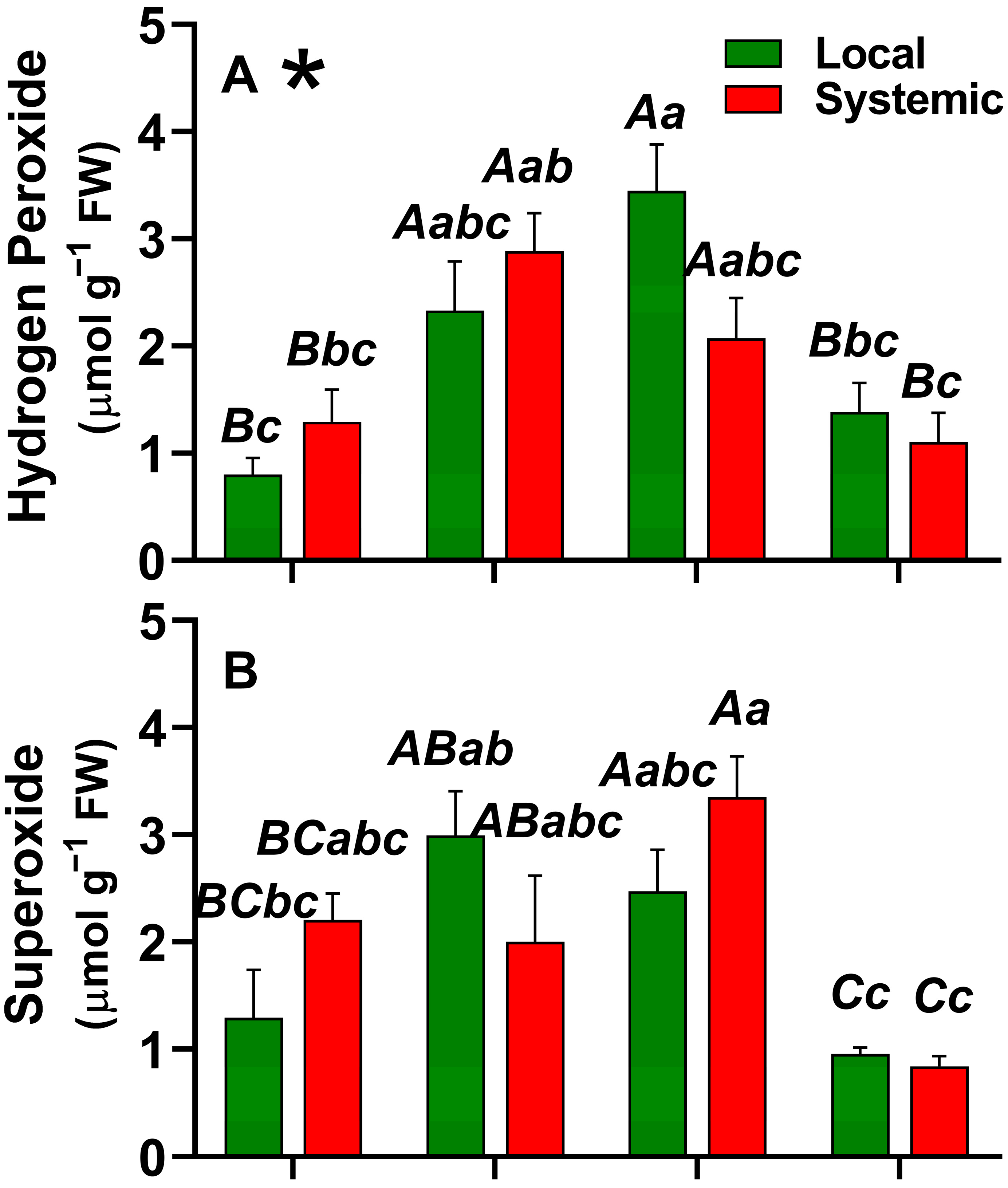
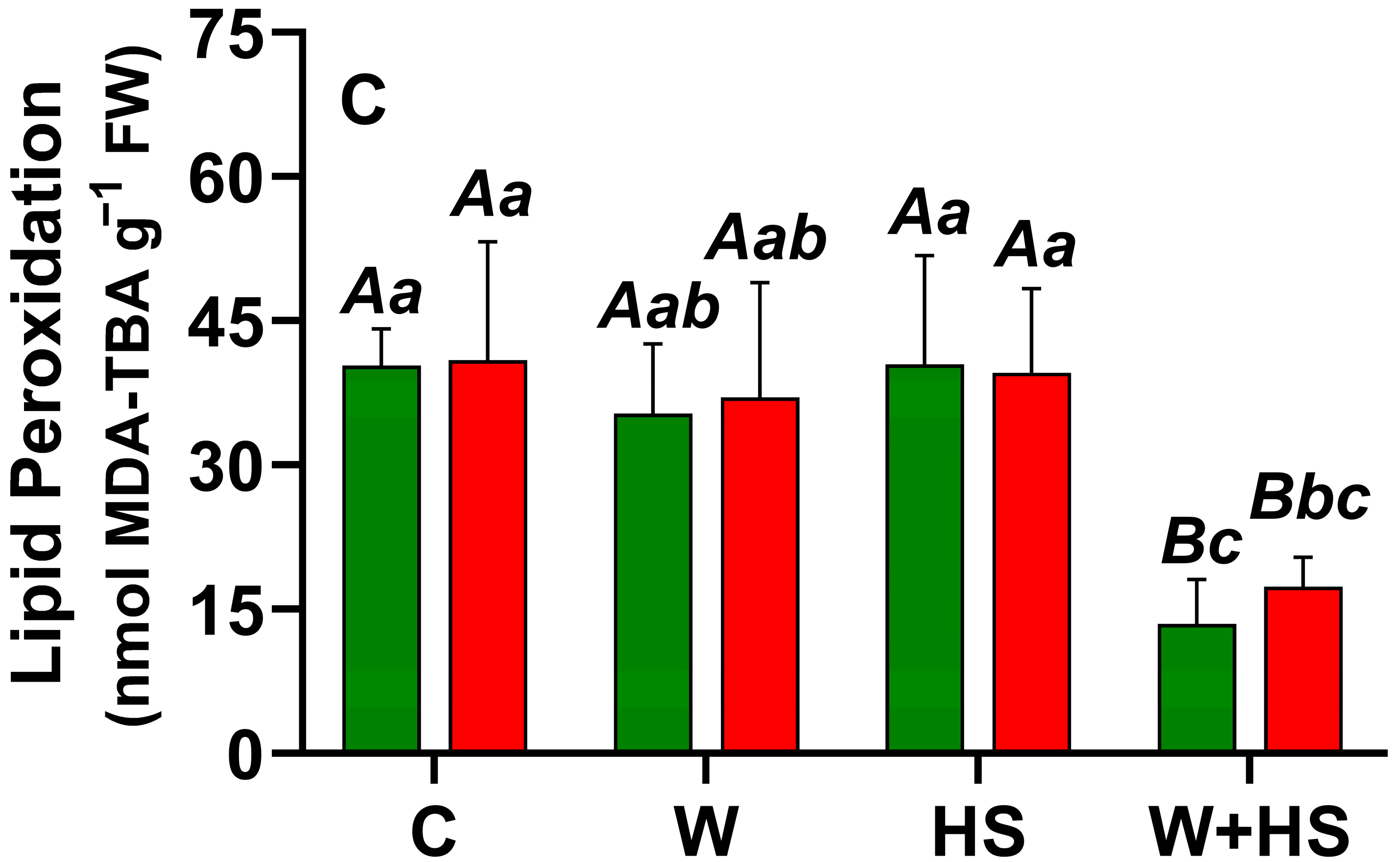
2.1. Local and Systemic ROS Responses
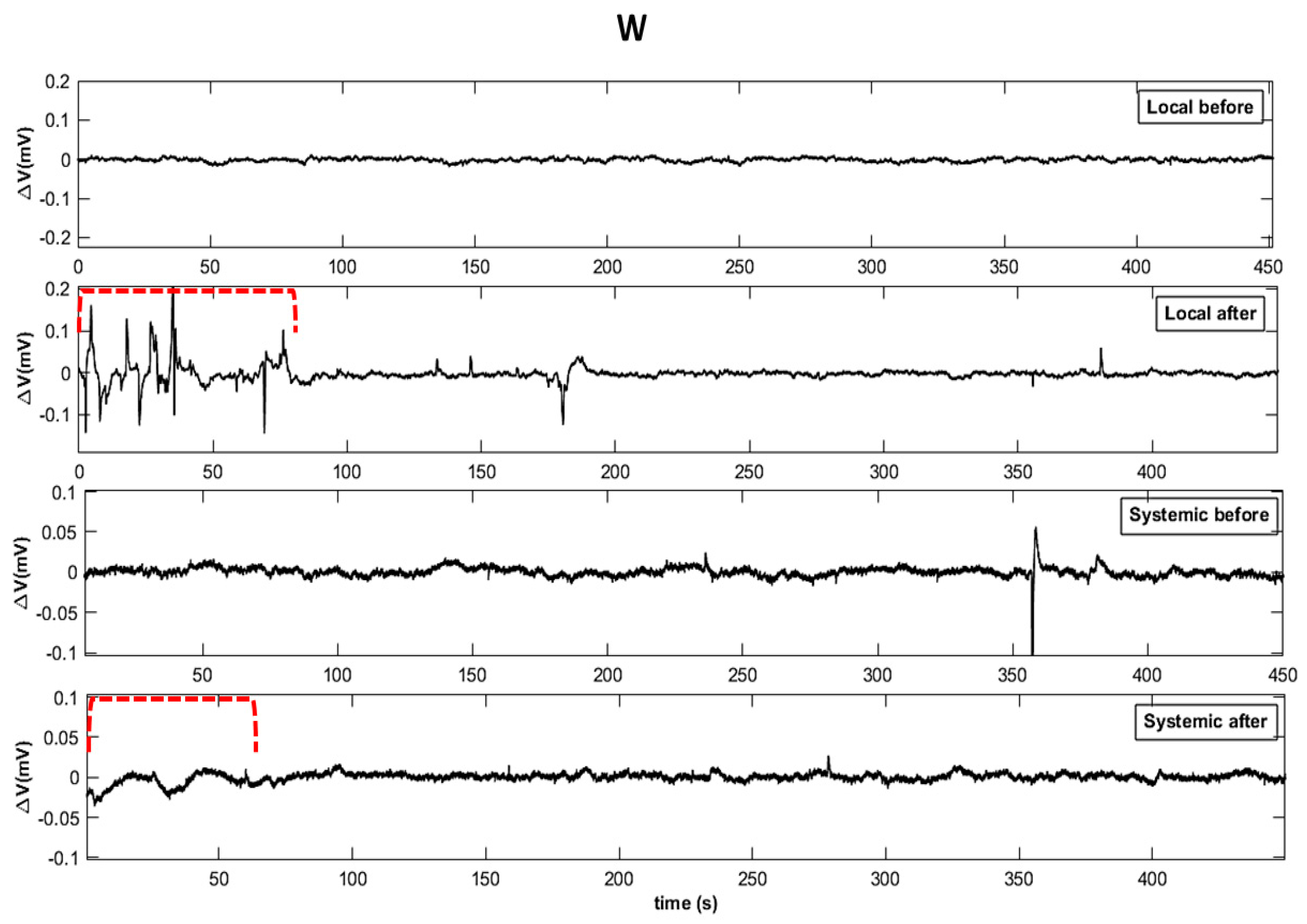
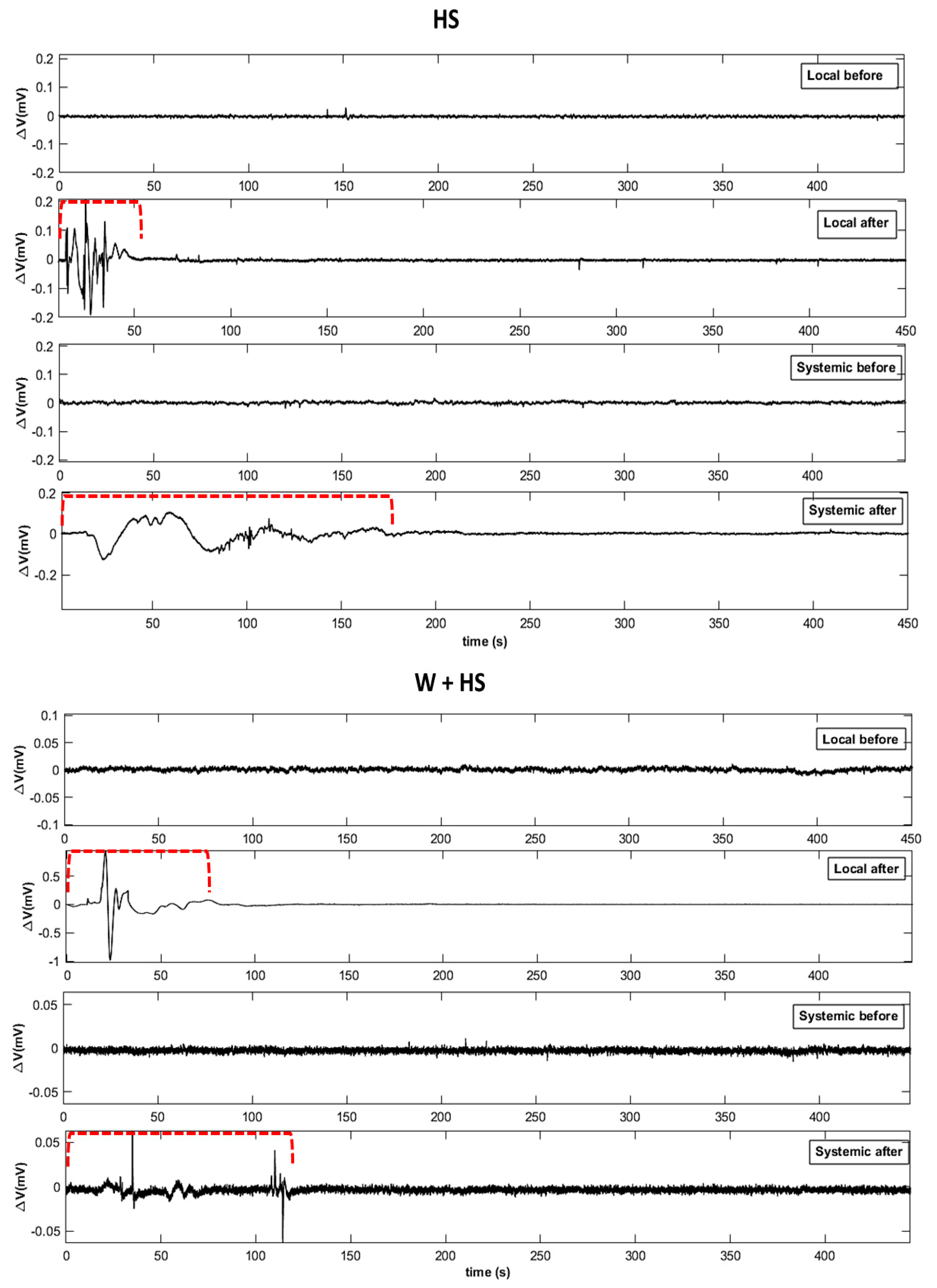
2.2. Electrome Dynamics
2.2.1. Visual Analysis
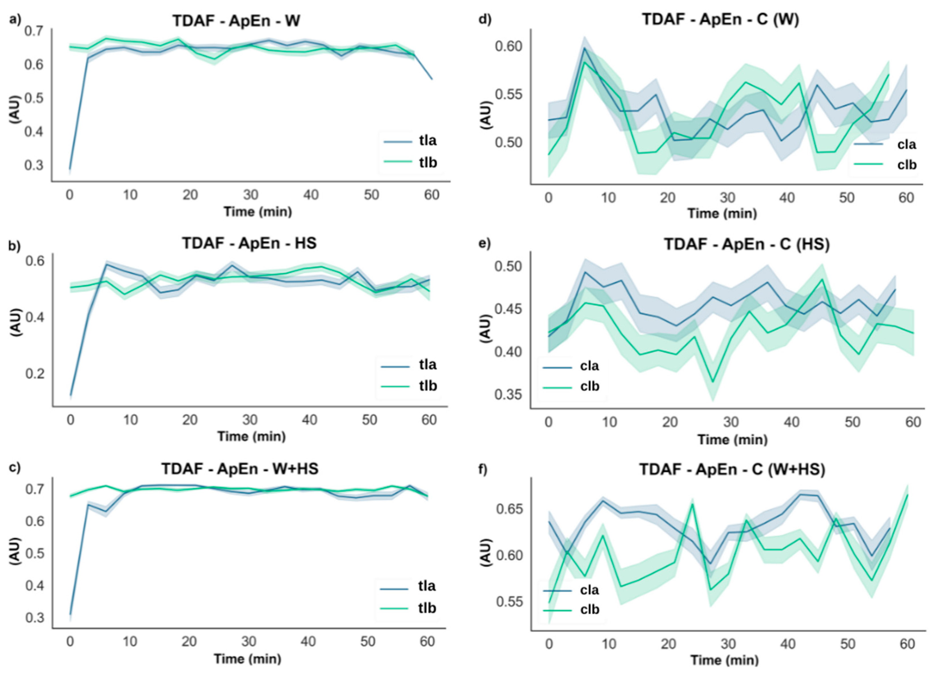
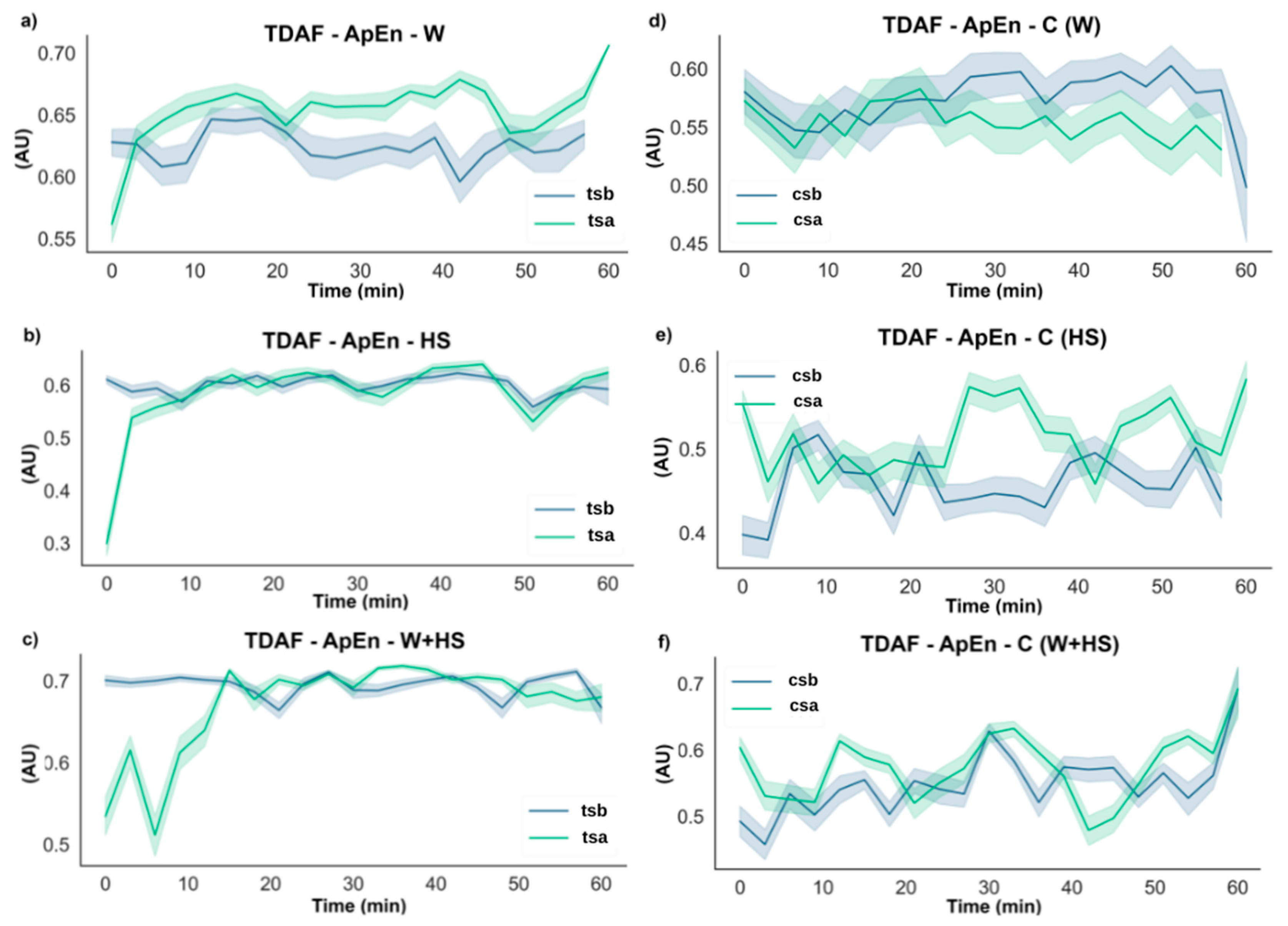
2.2.2. ApEn
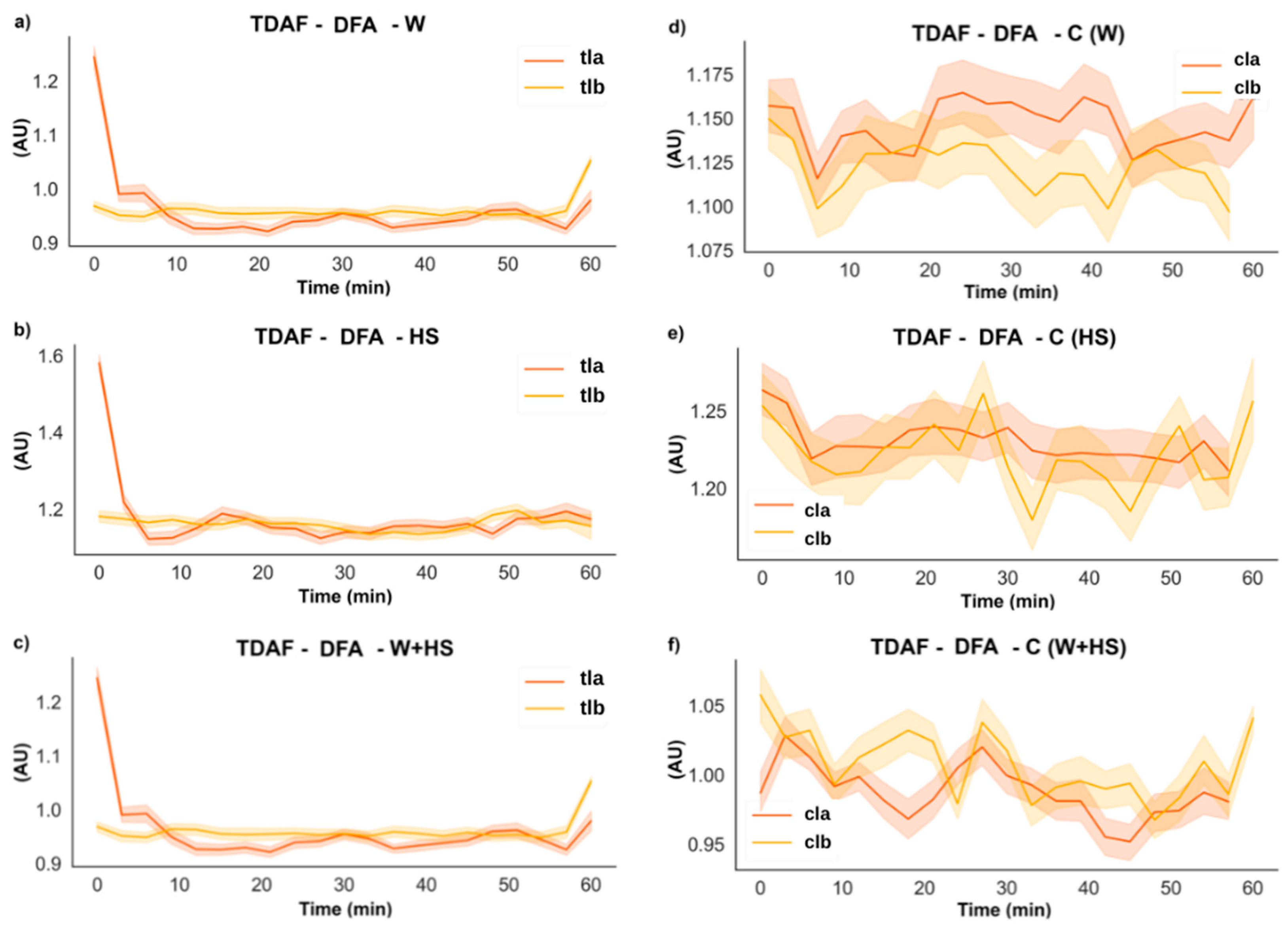
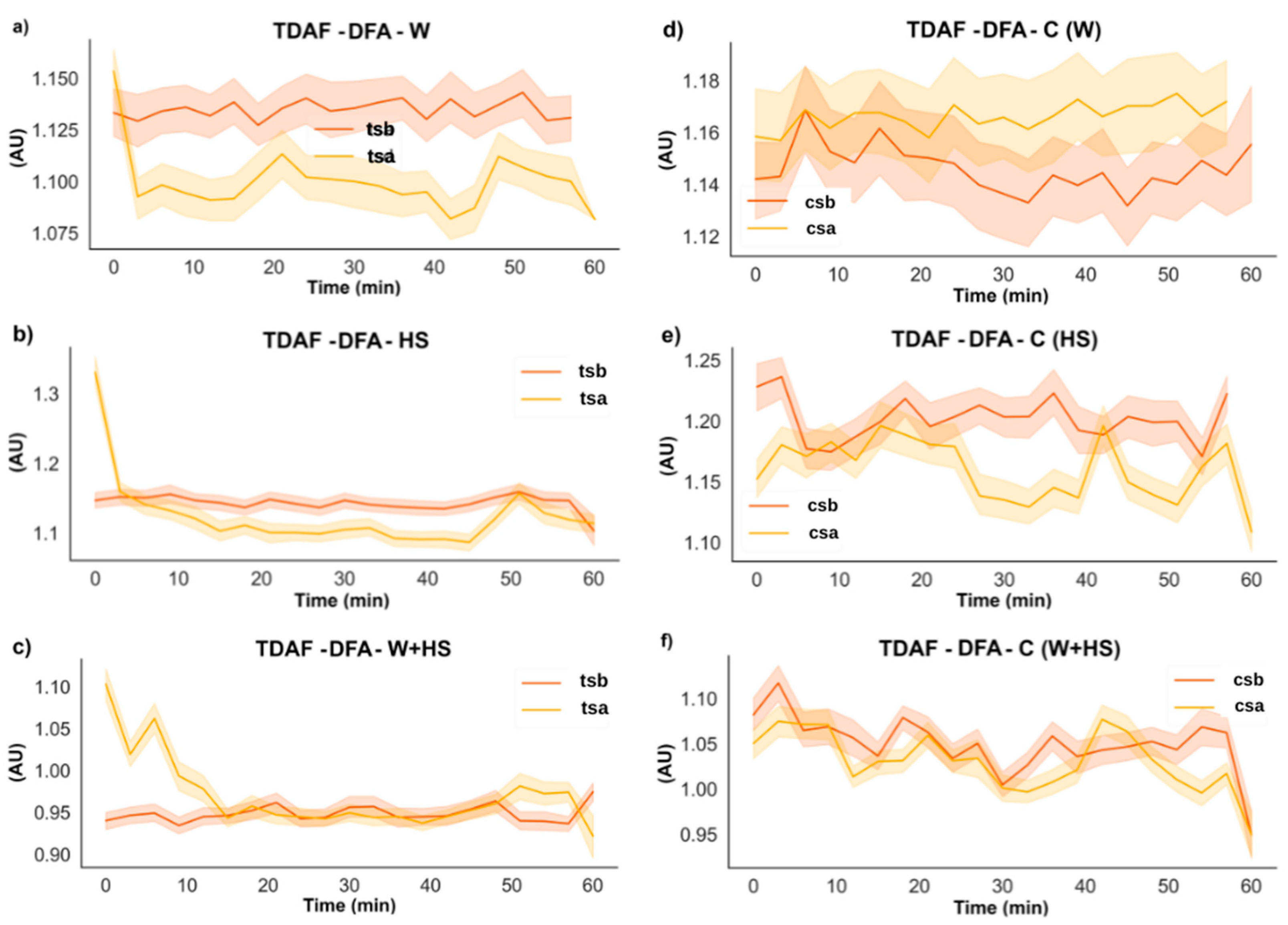
2.2.3. DFA
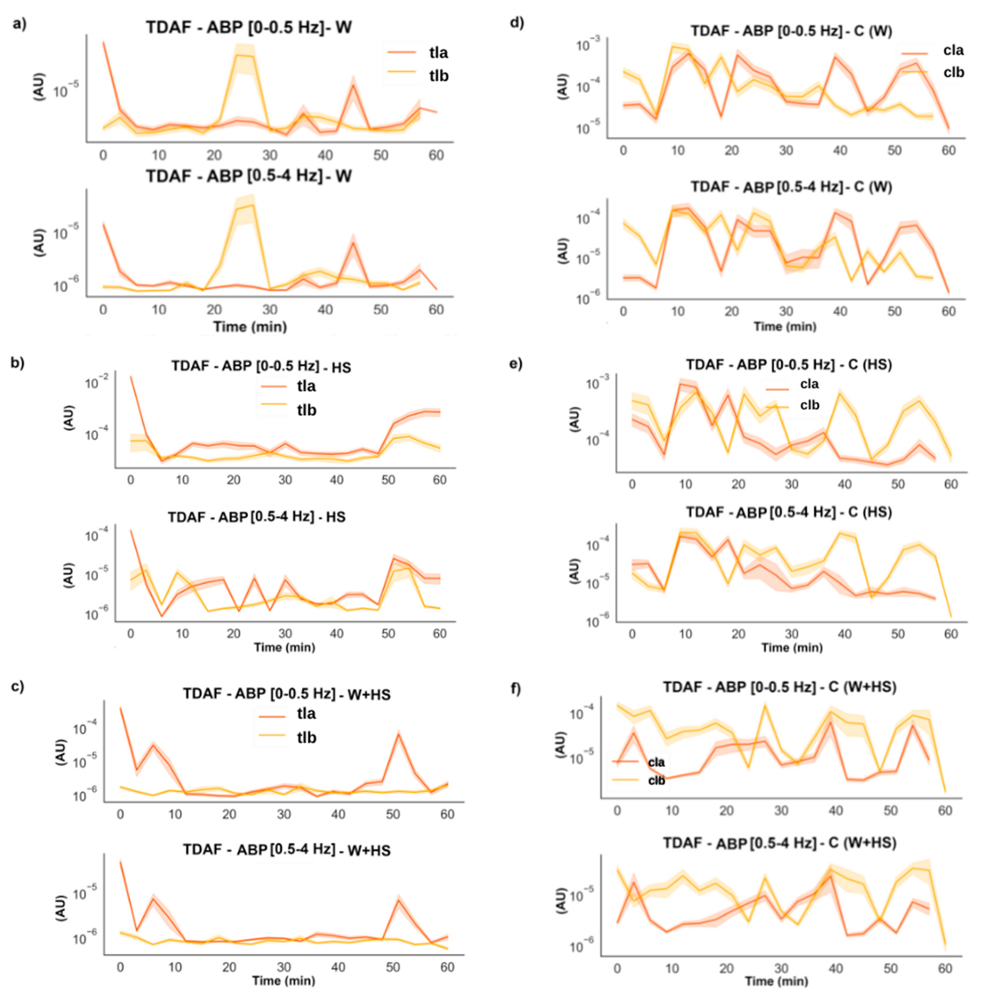
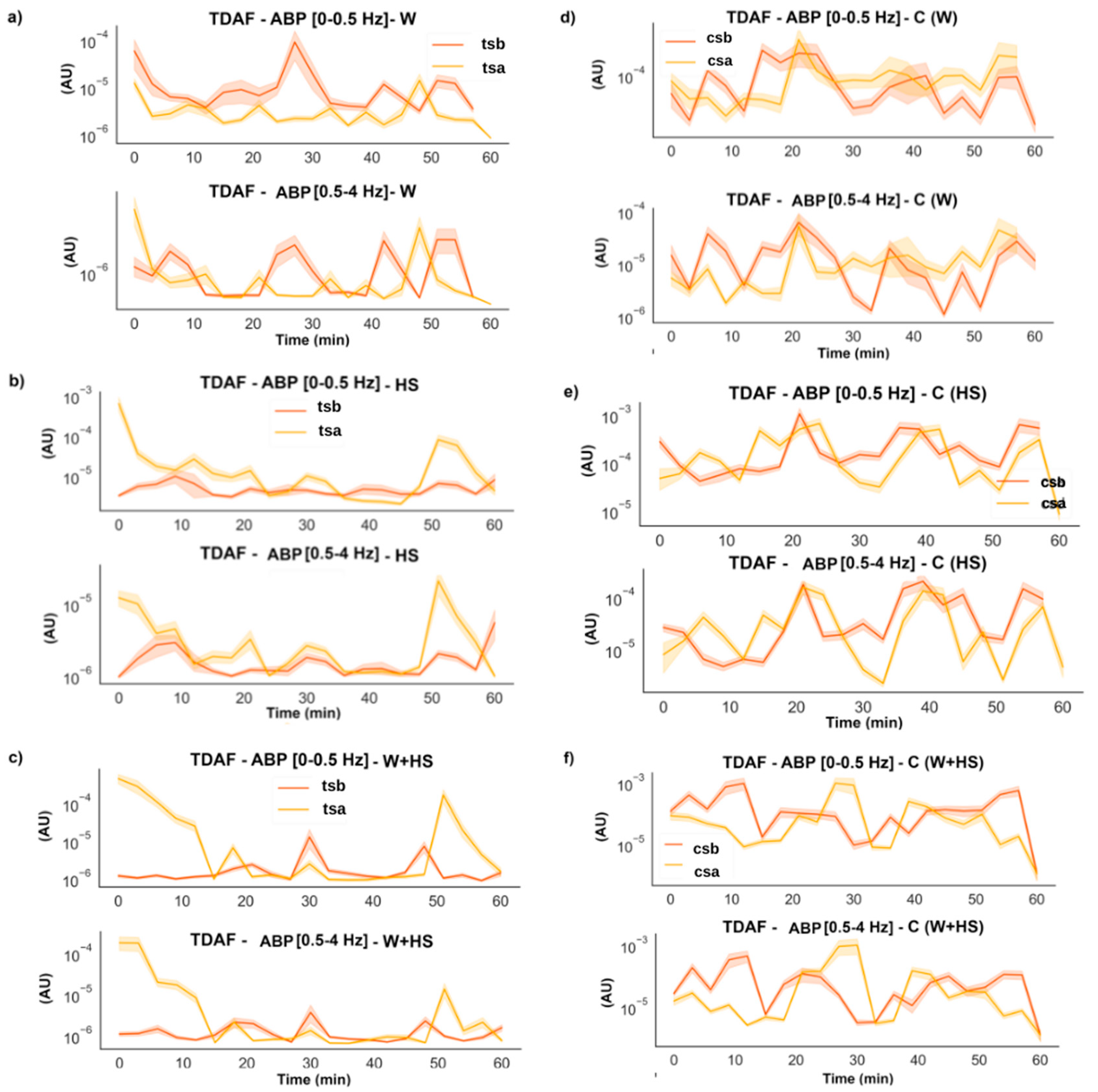
2.2.4. Average Band Power (ABP)
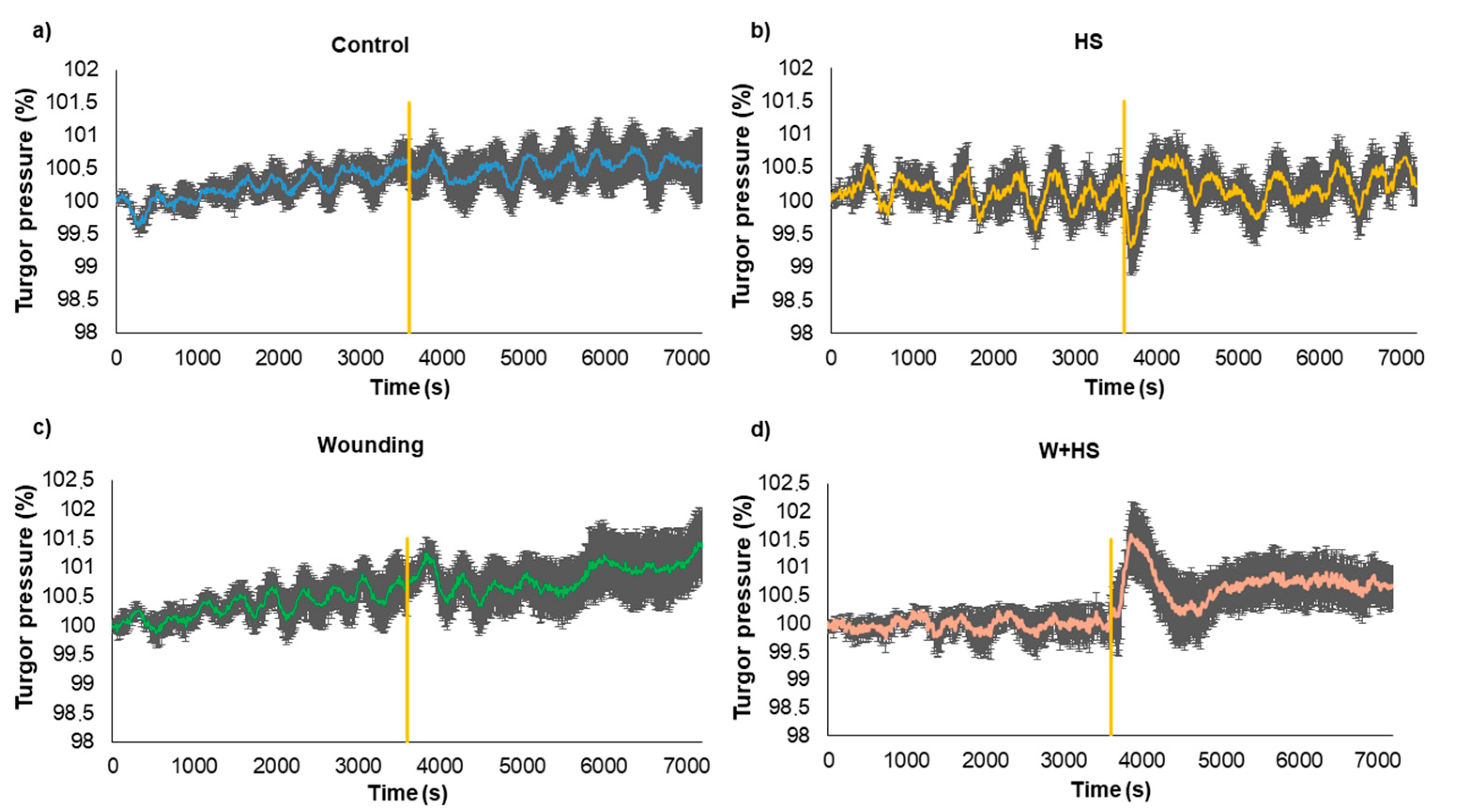
2.3. Measures of Turgor Pressure Variation
3. Discussion
4. Materials and Methods
4.1. Plant Material and Growing Conditions
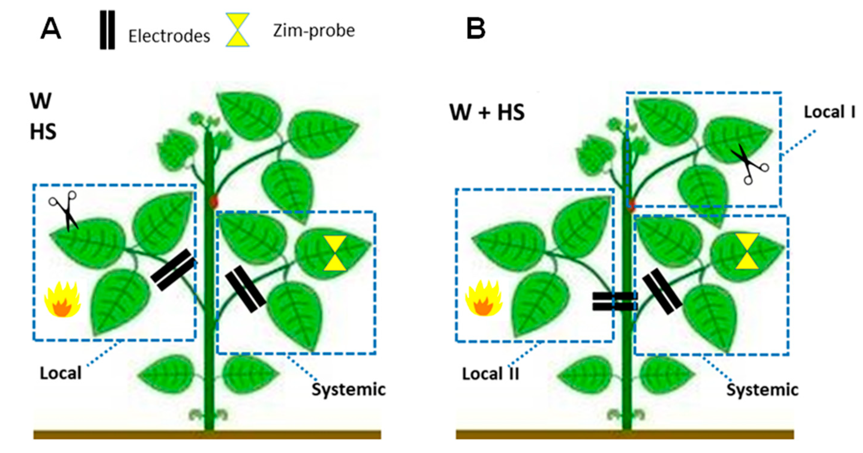
4.2. Experimental Design and Evaluation of the Dynamics of Systemic Responses Induced by Simple and Combined Stimuli
- Essay I—Heat shock (HS): The heat shock stimulus (HS) was applied by placing a flame approximately 10 cm from the central leaflet for 20 s. Measurements in unstimulated (control) plants were also obtained. Leaf temperature was measured with an infrared camera (FLIR Systems) on local leaves before and after stimulation to have an idea of leaf temperature variation during the test. According to the measurements, after stimulation, the local leaf temperature increased by an average of ±23 °C (data not shown).
- Essay II—Wounding (W): With calibrated scissors, 2 cm cuts in the central leaflet of the second trifoliate leaf were made to induce systemic wound signaling and response.
- Essay III—Heat shock + Wounding (HS+W): The stimuli were applied simultaneously to different leaves of the same plant to induce a signaling and systemic response to the combined stimulus. The 2 cm cut was applied to the third leaflet and the application of thermal shock was to the second leaflet for 20 s.
4.3. Quantification of ROS and Lipid Peroxidation
4.4. Electrome Acquisition and Analysis
4.4.1. Electrophytogram (EPG)
4.4.2. Electrophysiological Analyzes
Visual Inspection
Analysis of the Dispersion of Features over Time (Time Dispersion Analysis of Features—TDAF)
Detrended Fluctuation Analysis (DFA)
Average Band Power (Average Band Power—ABP)
Approximate Entropy
4.5. Measurements of Turgor Pressure Variation
4.6. Statistical Analysis
5. Conclusions
Author Contributions
Funding
Institutional Review Board Statement
Data Availability Statement
Acknowledgments
Conflicts of Interest
References
- Kollist, H.; Zandalinas, S.I.; Sengupta, S.; Nuhkat, M.; Kangasjärvi, J.; Mittler, R. Rapid Responses to Abiotic Stress: Priming the Landscape for the Signal Transduction Network. Trends Plant Sci. 2018, 24, 25–37. [Google Scholar] [CrossRef] [PubMed] [Green Version]
- Hilleary, R.; Gilroy, S. Systemic signaling in response to wounding and pathogens. Curr. Opin. Plant Biol. 2018, 43, 57–62. [Google Scholar] [CrossRef]
- Balfagón, D.; Sengupta, S.; Gómez-Cadenas, A.; Fritschi, F.B.; Azad, R.K.; Mittler, R.; Zandalinas, S.I. Jasmonic Acid Is Required for Plant Acclimation to a Combination of High Light and Heat Stress. Plant Physiol. 2019, 181, 1668–1682. [Google Scholar] [CrossRef] [PubMed] [Green Version]
- Choi, W.-G.; Hilleary, R.; Swanson, S.J.; Kim, S.-H.; Gilroy, S. Rapid, Long-Distance Electrical and Calcium Signaling in Plants. Annu. Rev. Plant Biol. 2016, 67, 287–307. [Google Scholar] [CrossRef] [PubMed]
- Johns, S.; Hagihara, T.; Toyota, M.; Gilroy, S. The fast and the furious: Rapid long-range signaling in plants. Plant Physiol. 2021, 185, 694–706. [Google Scholar] [CrossRef] [PubMed]
- Fichman, Y.; Mittler, R. Rapid systemic signaling during abiotic and biotic stresses: Is the ROS wave master of all trades? Plant J. 2020, 102, 887–896. [Google Scholar] [CrossRef] [Green Version]
- Huber, A.E.; Bauerle, T.L. Long-distance plant signaling pathways in response to multiple stressors: The gap in knowledge. J. Exp. Bot. 2016, 67, 2063–2079. [Google Scholar] [CrossRef] [Green Version]
- Sukhov, V.; Sukhova, E.; Vodeneev, V. Long-distance electrical signals as a link between the local action of stressors and the systemic physiological responses in higher plants. Prog. Biophys. Mol. Biol. 2018, 146, 63–84. [Google Scholar] [CrossRef]
- Fromm, J.; Hajirezaei, M.-R.; Becker, V.K.; Lautner, S. Electrical signaling along the phloem and its physiological responses in the maize leaf. Front. Plant Sci. 2013, 4, 239. [Google Scholar] [CrossRef] [Green Version]
- Choi, W.-G.; Miller, G.; Wallace, I.; Harper, J.; Mittler, R.; Gilroy, S. Orchestrating rapid long-distance signaling in plants with Ca2+, ROS and electrical signals. Plant J. 2017, 90, 698–707. [Google Scholar] [CrossRef] [Green Version]
- De Loof, A. The cell’s self-generated “electrome”: The biophysical essence of the immaterial dimension of Life? Commun. Integr. Biol. 2016, 9, e1197446. [Google Scholar] [CrossRef] [PubMed] [Green Version]
- De Toledo, G.R.A.; Parise, A.G.; Simmi, F.Z.; Costa, A.V.L.; Senko, L.G.S.; Debono, M.-W.; Souza, G.M. Plant electrome: The electrical dimension of plant life. Theor. Exp. Plant Physiol. 2019, 31, 21–46. [Google Scholar] [CrossRef]
- Debono, M.-W. Electrome & Cognition Modes in Plants: A Transdisciplinary Approach to the Eco-Sensitiveness of the World. Transdiscipl. J. Eng. Sci. 2020, 11, 213–239. [Google Scholar] [CrossRef]
- Saraiva, G.F.R.; Ferreira, A.S.; Souza, G.M. Osmotic stress decreases complexity underlying the electrophysiological dynamic in soybean. Plant Biol. 2017, 19, 702–708. [Google Scholar] [CrossRef]
- Simmi, F.; Dallagnol, L.; Ferreira, A.; Pereira, D.; Souza, G. Electrome alterations in a plant-pathogen system: Toward early diagnosis. Bioelectrochemistry 2020, 133, 107493. [Google Scholar] [CrossRef]
- Parise, A.G.; Reissig, G.N.; Basso, L.F.; Senko, L.G.S.; Oliveira, T.F.d.C.; de Toledo, G.R.A.; Ferreira, A.S.; Souza, G.M. Detection of Different Hosts From a Distance Alters the Behaviour and Bioelectrical Activity of Cuscuta racemosa. Front. Plant Sci. 2021, 12, 409. [Google Scholar] [CrossRef]
- Reissig, G.N.; Oliveira, T.F.d.C.; de Oliveira, R.P.; Posso, D.A.; Parise, A.G.; Nava, D.E.; Souza, G.M. Fruit Herbivory Alters Plant Electrome: Evidence for Fruit-Shoot Long-Distance Electrical Signaling in Tomato Plants. Front. Sustain. Food Syst. 2021, 5, 244. [Google Scholar] [CrossRef]
- Reissig, G.N.; Oliveira, T.F.d.C.; Costa, V.L.; Parise, A.G.; Pereira, D.R.; Souza, G.M. Machine Learning for Automatic Classification of Tomato Ripening Stages Using Electrophysiological Recordings. Front. Sustain. Food Syst. 2021, 5, 696829. [Google Scholar] [CrossRef]
- Pereira, D.R.; Papa, J.P.; Saraiva, G.F.R.; Souza, G.M. Automatic classification of plant electrophysiological responses to environmental stimuli using machine learning and interval arithmetic. Comput. Electron. Agric. 2018, 145, 35–42. [Google Scholar] [CrossRef] [Green Version]
- Christmann, A.; Grill, E.; Huang, J. Hydraulic signals in long-distance signaling. Curr. Opin. Plant Biol. 2013, 16, 293–300. [Google Scholar] [CrossRef]
- Malone, M. Hydraulic signals. Philos. Trans. R. Soc. B Biol. Sci. 1993, 341, 33–39. [Google Scholar] [CrossRef]
- Bramley, H.; Turner, D.; Tyerman, S.; Turner, N. Water Flow in the Roots of Crop Species: The Influence of Root Structure, Aquaporin Activity, and Waterlogging. Adv. Agron. 2007, 96, 133–196. [Google Scholar] [CrossRef]
- Hamilton, E.S.; Schlegel, A.M.; Haswell, E.S. United in Diversity: Mechanosensitive Ion Channels in Plants. Annu. Rev. Plant Biol. 2015, 66, 113–137. [Google Scholar] [CrossRef] [PubMed] [Green Version]
- Amien, S.; Kliwer, I.; Márton, M.L.; Debener, T.; Geiger, D.; Becker, D.; Dresselhaus, T. Defensin-Like ZmES4 Mediates Pollen Tube Burst in Maize via Opening of the Potassium Channel KZM1. PLoS Biol. 2010, 8, e1000388. [Google Scholar] [CrossRef] [PubMed] [Green Version]
- Zandalinas, S.I.; Fichman, Y.; Devireddy, A.R.; Sengupta, S.; Azad, R.K.; Mittler, R. Systemic signaling during abiotic stress combination in plants. Proc. Natl. Acad. Sci. USA 2020, 117, 13810–13820. [Google Scholar] [CrossRef]
- Fichman, Y.; Mittler, R. Integration of electric, calcium, reactive oxygen species and hydraulic signals during rapid systemic signaling in plants. Plant J. 2021, 107, 7–20. [Google Scholar] [CrossRef] [PubMed]
- Suzuki, N.; Rivero, R.M.; Shulaev, V.; Blumwald, E.; Mittler, R. Abiotic and biotic stress combinations. New Phytol. 2014, 203, 32–43. [Google Scholar] [CrossRef]
- Zandalinas, S.; Sengupta, S.; Burks, D.; Azad, R.K.; Mittler, R. Identification and characterization of a core set of ROS wave-associated transcripts involved in the systemic acquired acclimation response of Arabidopsis to excess light. Plant J. 2018, 98, 126–141. [Google Scholar] [CrossRef]
- Midzi, J.; Jeffery, D.W.; Baumann, U.; Rogiers, S.; Tyerman, S.D.; Pagay, V. Stress-Induced Volatile Emissions and Signalling in Inter-Plant Communication. Plants 2022, 11, 2566. [Google Scholar] [CrossRef]
- Balfagón, D.; Terán, F.; Oliveira, T.D.R.D.; Santa-Catarina, C.; Gómez-Cadenas, A. Citrus rootstocks modify scion antioxidant system under drought and heat stress combination. Plant Cell Rep. 2021, 41, 593–602. [Google Scholar] [CrossRef]
- Mudrilov, M.; Ladeynova, M.; Grinberg, M.; Balalaeva, I.; Vodeneev, V. Electrical Signaling of Plants under Abiotic Stressors: Transmission of Stimulus-Specific Information. Int. J. Mol. Sci. 2021, 22, 10715. [Google Scholar] [CrossRef] [PubMed]
- Mittler, R. Abiotic stress, the field environment and stress combination. Trends Plant Sci. 2006, 11, 15–19. [Google Scholar] [CrossRef] [PubMed]
- Rizhsky, L.; Liang, H.; Shuman, J.; Shulaev, V.; Davletova, S.; Mittler, R. When Defense Pathways Collide. The Response of Arabidopsis to a Combination of Drought and Heat Stress. Plant Physiol. 2004, 134, 1683–1696. [Google Scholar] [CrossRef] [PubMed] [Green Version]
- Suzuki, N.; Bassil, E.; Hamilton, J.S.; Inupakutika, M.A.; Zandalinas, S.I.; Tripathy, D.; Luo, Y.; Dion, E.; Fukui, G.; Kumazaki, A.; et al. ABA Is Required for Plant Acclimation to a Combination of Salt and Heat Stress. PLoS ONE 2016, 11, e0147625. [Google Scholar] [CrossRef] [Green Version]
- Vuralhan-Eckert, J.; Lautner, S.; Fromm, J. Effect of simultaneously induced environmental stimuli on electrical signalling and gas exchange in maize plants. J. Plant Physiol. 2018, 223, 32–36. [Google Scholar] [CrossRef]
- Souza, G.M.; Ferreira, A.S.; Saraiva, G.F.R.; Toledo, G.R.A. Plant “electrome” can be pushed toward a self-organized critical state by external cues: Evidences from a study with soybean seedlings subject to different environmental conditions. Plant Signal. Behav. 2017, 12, e1290040. [Google Scholar] [CrossRef] [Green Version]
- Malone, M.; Stankovic, B. Surface potentials and hydraulic signals in wheat leaves following localized wounding by heat. Plant, Cell Environ. 1991, 14, 431–436. [Google Scholar] [CrossRef]
- Malone, M. Rapid, long-distance signal transmission in higher plants. Adv. Bot. Res. 1996, 22, 163–228. [Google Scholar]
- Peláez-Vico, M.; Fichman, Y.; Zandalinas, S.I.; Van Breusegem, F.; Karpiński, S.M.; Mittler, R. ROS and redox regulation of cell-to-cell and systemic signaling in plants during stress. Free. Radic. Biol. Med. 2022, 193, 354–362. [Google Scholar] [CrossRef]
- Zandalinas, S.I.; Sales, C.; Beltrán, J.; Gómez-Cadenas, A.; Arbona, V. Activation of Secondary Metabolism in Citrus Plants Is Associated to Sensitivity to Combined Drought and High Temperatures. Front. Plant Sci. 2017, 7, 1954. [Google Scholar] [CrossRef] [Green Version]
- Devireddy, A.R.; Zandalinas, S.I.; Gómez-Cadenas, A.; Blumwald, E.; Mittler, R. Coordinating the overall stomatal response of plants: Rapid leaf-to-leaf communication during light stress. Sci. Signal. 2018, 11, 1126. [Google Scholar] [CrossRef] [Green Version]
- Peng, C.K.; Havlin, S.; Stanley, H.E.; Goldberger, A.G. Quantification of scaling exponents and crossover phenomena in nonstationary heartbeat time series. Chaos: An interdisciplinary journal of nonlinear. Science 1995, 5, 82–87. [Google Scholar]
- Dvořák, P.; Krasylenko, Y.; Zeiner, A.; Šamaj, J.; Takáč, T. Signaling Toward Reactive Oxygen Species-Scavenging Enzymes in Plants. Front. Plant Sci. 2021, 11, 2178. [Google Scholar] [CrossRef]
- Kranner, I.; Minibayeva, F.; Beckett, R.; Seal, C. What is stress? Concepts, definitions and applications in seed science. New Phytol. 2010, 188, 655–673. [Google Scholar] [CrossRef]
- Parise, A.G.; de Toledo, G.R.A.; Oliveira, T.F.d.C.; Souza, G.M.; Castiello, U.; Gagliano, M.; Marder, M. Do plants pay attention? A possible phenomenological-empirical approach. Prog. Biophys. Mol. Biol. 2022, 173, 11–23. [Google Scholar] [CrossRef]
- Marder, M. Plant intelligence and attention. Plant Signal. Behav. 2013, 8, e23902. [Google Scholar] [CrossRef] [PubMed] [Green Version]
- Hoagland, D.R.; Arnon, D.I. Water-Culture Method Grow. Plants Without Soil. Circ. Calif. Agric. Exp. Stn. 1950, 347, 1–39. [Google Scholar]
- Li, C.; Bai, T.; Ma, F.; Han, M. Hypoxia tolerance and adaptation of anaerobic respiration to hypoxia stress in two Malus species. Sci. Hortic. 2010, 124, 274–279. [Google Scholar] [CrossRef]
- Velikova, V.; Yordanov, I.; Edreva, A. Oxidative stress and some antioxidant systems in acid rain-treated bean plants: Protective role of exogenous polyamines. Plant Sci. 2000, 151, 59–66. [Google Scholar] [CrossRef]
- Volkov, A.; Haack, R. Insect-induced biolectrochemical signals in potato plants. Bioelectrochemistry Bioenerg. 1995, 37, 55–60. [Google Scholar] [CrossRef]
- Jorgensen, B. The Theory of Dispersion Models; CRC Press: Boca Raton, FL, USA, 1997. [Google Scholar]
- Hardstone, R.; Poil, S.-S.; Schiavone, G.; Jansen, R.; Nikulin, V.V.; Mansvelder, H.D.; Linkenkaer-Hansen, K. Detrended Fluctuation Analysis: A Scale-Free View on Neuronal Oscillations. Front. Physiol. 2012, 3, 450. [Google Scholar] [CrossRef] [PubMed] [Green Version]
- Abhang, P.A.; Gawali, B.W.; Mehrotra, S.C. Technological Basics of EEG Recording and Operation of Apparatus. In Introduction to EEG- and Speech-Based Emotion Recognition; Abhang, P.A., Gawali, B., Mehrotra, S.C., Eds.; Academic Press: Cambridge, MA, USA, 2016; pp. 19–50. [Google Scholar]
- Delimayanti, M.K.; Purnama, B.; Nguyen, N.G.; Faisal, M.R.; Mahmudah, K.R.; Indriani, F.; Kubo, M.; Satou, K. Classification of Brainwaves for Sleep Stages by High-Dimensional FFT Features from EEG Signals. Appl. Sci. 2020, 10, 1797. [Google Scholar] [CrossRef] [Green Version]
- Evans, J.R. Neurofeedback. In Encyclopedia of the Human Brain; Elsevier: Amsterdam, The Netherlands, 2002; pp. 465–477. [Google Scholar]
- Heraz, A.; Razaki, R.; Frasson, C. Using machine learning to predict learner emotional state from brainwaves. In Proceedings of the Seventh IEEE International Conference on Advanced Learning Technologies (ICALT 2007), Niigata, Japan, 18–20 July 2007. [Google Scholar]
- Kora, P.; Meenakshi, K.; Swaraja, K.; Rajani, A.; Raju, M.S. EEG based interpretation of human brain activity during yoga and meditation using machine learning: A systematic review. Complement. Ther. Clin. Pr. 2021, 43, 101329. [Google Scholar] [CrossRef] [PubMed]
- Savadkoohi, M.; Oladunni, T.; Thompson, L. A machine learning approach to epileptic seizure prediction using Electroencephalogram (EEG) Signal. Biocybern. Biomed. Eng. 2020, 40, 1328–1341. [Google Scholar] [CrossRef] [PubMed]
- White, N.E.; Richards, L.M. Alpha–theta neurotherapy and the neurobehavioral treatment of addictions, mood disorders and trauma. In Introduction to Quantitative EEG and Neurofeedback; Elsevier: Amsterdam, The Netherlands, 2009; pp. 143–166. [Google Scholar]
- Press, W.H.; Flannery, B.P.; Teukolsky, S.A.; Vetterling, W.T. Numerical Recipes in Pascal (First Edition): The Art of Scientific Computing; Cambridge University Press: Cambridge, UK, 1989. [Google Scholar]
- Costa, M.; Goldberger, A.L.; Peng, C.-K. Multiscale entropy analysis of biological signals. Phys. Rev. E 2005, 71, 021906. [Google Scholar] [CrossRef] [Green Version]
- Ocak, H. Automatic detection of epileptic seizures in EEG using discrete wavelet transform and approximate entropy. Expert Syst. Appl. 2009, 36, 2027–2036. [Google Scholar] [CrossRef]
- Pincus, S.M. Approximate entropy as a measure of system complexity. Proc. Natl. Acad. Sci. USA 1991, 88, 2297–2301. [Google Scholar] [CrossRef] [Green Version]
- Pincus, S.M. Approximate entropy (ApEn) as a complexity measure. Chaos Interdiscip. J. Nonlinear Sci. 1995, 5, 110–117. [Google Scholar] [CrossRef]
- Pincus, S.M.; Goldberger, A.L. Physiological time-series analysis: What does regularity quantify? Am. J. Physiol. Circ. Physiol. 1994, 266, H1643–H16561994. [Google Scholar] [CrossRef]
- Zimmermann, M.R.; Maischak, H.; Mithofer, A.; Boland, W.; Felle, H.H. System Potentials, a Novel Electrical Long-Distance Apoplastic Signal in Plants, Induced by Wounding. Plant Physiol. 2009, 149, 1593–1600. [Google Scholar] [CrossRef] [Green Version]
- Zimmermann, U.; Bitter, R.; Marchiori, P.E.R.; Rüger, S.; Ehrenberger, W.; Sukhorukov, V.L.; Schüttler, A.; Ribeiro, R.V. A non-invasive plant-based probe for continuous monitoring of water stress in real time: A new tool for irrigation scheduling and deeper insight into drought and salinity stress physiology. Theor. Exp. Plant Physiol. 2013, 25, 2–11. [Google Scholar] [CrossRef]
- Baudouin, E.; Hancock, J.T. Nitric oxide signaling in plants. Front. Plant Sci. 2014, 4, 553. [Google Scholar] [CrossRef] [PubMed] [Green Version]
- Winter, N.; Kragler, F. Conceptual and Methodological Considerations on mRNA and Proteins as Intercellular and Long-Distance Signals. Plant Cell Physiol. 2018, 59, 1700–1713. [Google Scholar] [CrossRef] [PubMed] [Green Version]
- Barbier, F.F.; Dun, E.A.; Kerr, S.C.; Chabikwa, T.G.; Beveridge, C.A. An Update on the Signals Controlling Shoot Branching. Trends Plant Sci. 2019, 24, 220–236. [Google Scholar] [CrossRef]
- Zebelo, S.A.; Matsui, K.; Ozawa, R.; Maffei, M.E. Plasma membrane potential depolarization and cytosolic calcium flux are early events involved in tomato (Solanum lycopersicon) plant-to-plant communication. Plant Sci. 2012, 196, 93–100. [Google Scholar] [CrossRef]


Disclaimer/Publisher’s Note: The statements, opinions and data contained in all publications are solely those of the individual author(s) and contributor(s) and not of MDPI and/or the editor(s). MDPI and/or the editor(s) disclaim responsibility for any injury to people or property resulting from any ideas, methods, instructions or products referred to in the content. |
© 2023 by the authors. Licensee MDPI, Basel, Switzerland. This article is an open access article distributed under the terms and conditions of the Creative Commons Attribution (CC BY) license (https://creativecommons.org/licenses/by/4.0/).
Share and Cite
Costa, Á.V.L.; Oliveira, T.F.d.C.; Posso, D.A.; Reissig, G.N.; Parise, A.G.; Barros, W.S.; Souza, G.M. Systemic Signals Induced by Single and Combined Abiotic Stimuli in Common Bean Plants. Plants 2023, 12, 924. https://doi.org/10.3390/plants12040924
Costa ÁVL, Oliveira TFdC, Posso DA, Reissig GN, Parise AG, Barros WS, Souza GM. Systemic Signals Induced by Single and Combined Abiotic Stimuli in Common Bean Plants. Plants. 2023; 12(4):924. https://doi.org/10.3390/plants12040924
Chicago/Turabian StyleCosta, Ádrya Vanessa Lira, Thiago Francisco de Carvalho Oliveira, Douglas Antônio Posso, Gabriela Niemeyer Reissig, André Geremia Parise, Willian Silva Barros, and Gustavo Maia Souza. 2023. "Systemic Signals Induced by Single and Combined Abiotic Stimuli in Common Bean Plants" Plants 12, no. 4: 924. https://doi.org/10.3390/plants12040924