
Selection of Soybean Genotypes under Drought and Saline Stress Conditions Using Manhattan Distance and TOPSIS

 ,
,  ,
,  , ,
, ,
Abstract
:1. Introduction
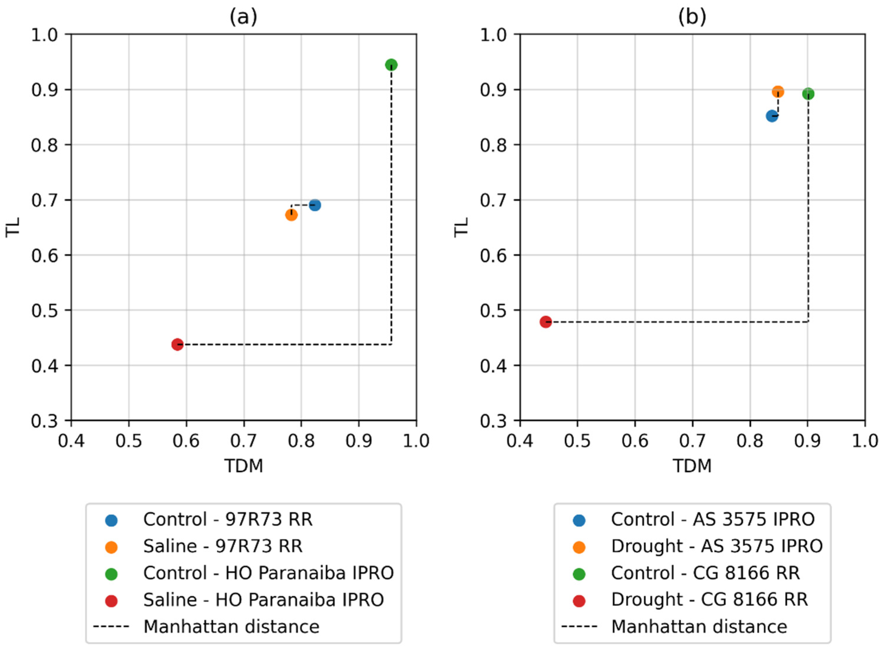
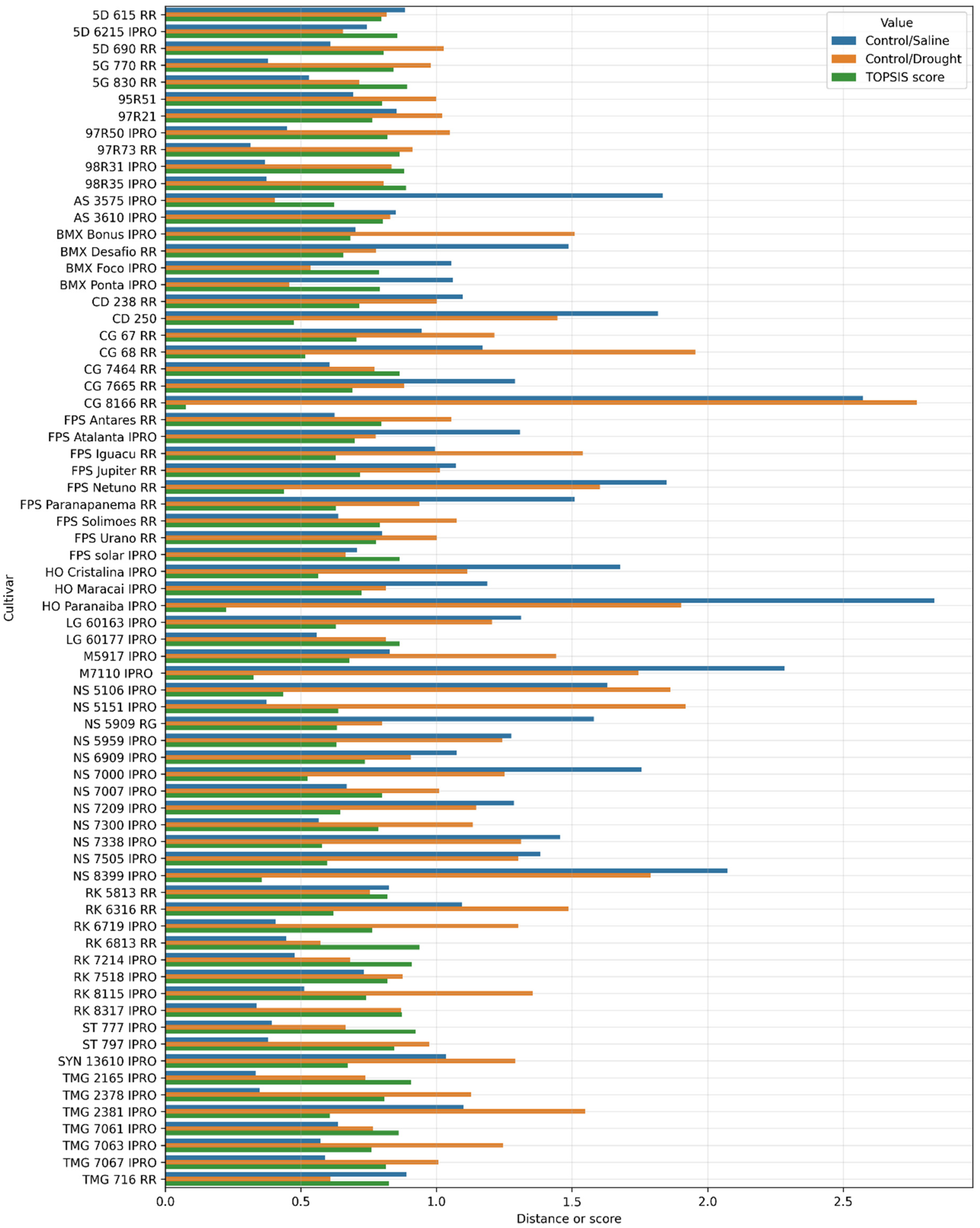
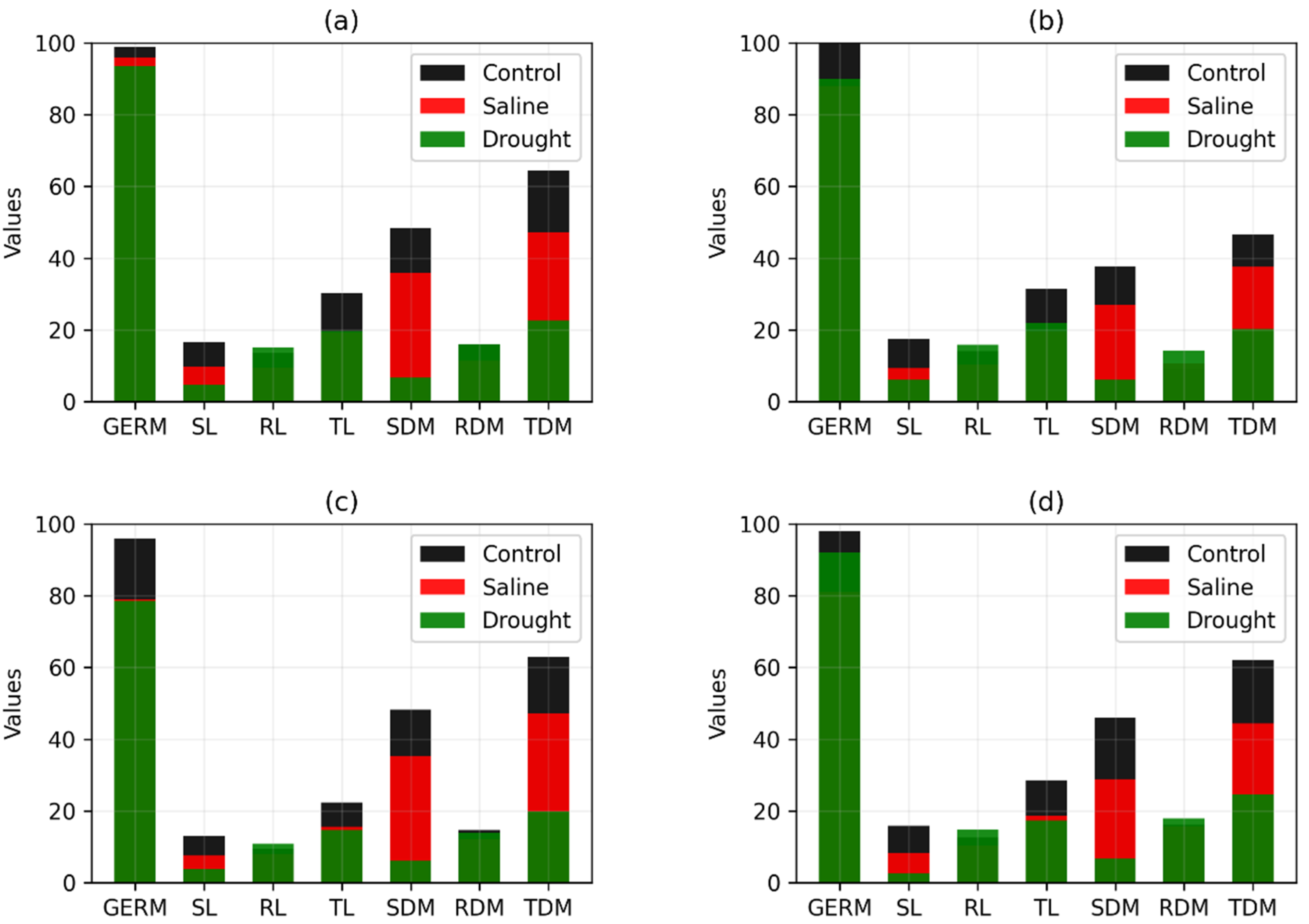
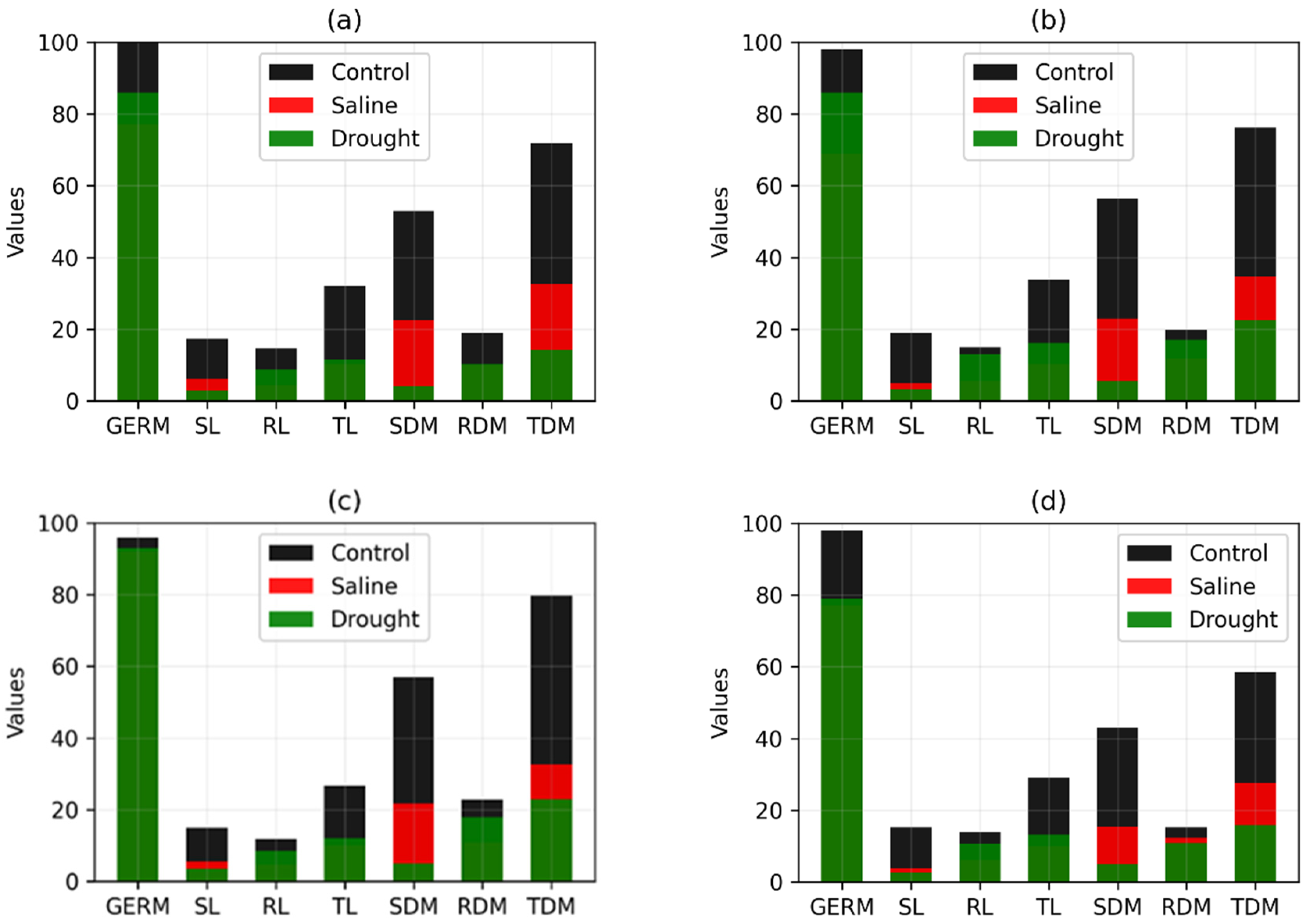
2. Results
3. Discussion
4. Materials and Methods
4.1. Plant Material and Stress Treatments
4.2. Germination Conditions and Measured Variables
4.3. Manhattan Distance and Similarity
4.4. TOPSIS
4.5. Proposed Approach
5. Conclusions
Author Contributions
Funding
Institutional Review Board Statement
Informed Consent Statement
Data Availability Statement
Conflicts of Interest
References
- Cattelan, A.J.; Dall’Agnol, A. The rapid soybean growth in Brazil. Oilseeds Fats Crops Lipids 2018, 25, 102. [Google Scholar] [CrossRef] [Green Version]
- Saidganieva, S.T.Q.; Yuldasheva, S.N.Q. Measures against the damage of the insects of the nightshades family in the Soybean plant. Asian J. Multidimens. Res. 2020, 9, 28–30. [Google Scholar] [CrossRef]
- Pagano, M.C.; Miransari, M. The importance of soybean production worldwide. In Abiotic and Biotic Stresses in Soybean Production; Academic Press: Cambridge, MA, USA, 2016; pp. 1–26. [Google Scholar] [CrossRef]
- Zuffo, A.M.; Steiner, F.; Aguilera, J.G.; Teodoro, P.E.; Teodoro, L.P.R.; Busch, A. Multi-trait stability index: A tool for simultaneous selection of soya bean genotypes in drought and saline stress. J. Agron. Crop Sci. 2020, 206, 815–822. [Google Scholar] [CrossRef]
- Steiner, F.; Zuffo, A.M.; Teodoro, P.E.; Aguilera, J.G.; Teodoro, L.P.R. Multivariate adaptability and stability of soya bean genotypes for abiotic stresses. J. Agron. Crop Sci. 2021, 207, 354–361. [Google Scholar] [CrossRef]
- Gheyi, H.R.; Dias, N.S.; Lacerda, C.F. Manejo da Salinidade na Agricultura: Estudos Básicos e Aplicados; INCT Sal: Fortaleza, Brazil, 2010; 472p. [Google Scholar]
- Patanè, C.; Saita, A.; Sortino, O. Comparative effects of salt and water stress on seed germination and early embryo growth in two cultivars of sweet sorghum. J. Agron. Crop Sci. 2013, 199, 30–37. [Google Scholar] [CrossRef]
- Steiner, F.; Zuffo, A.M.; Zoz, T.; Zoz, A.; Zoz, J. Drought tolerance of wheat and black oat crops at early stages of seedling growth. Rev. De Ciências Agrárias 2017, 40, 576–586. [Google Scholar] [CrossRef] [Green Version]
- Acosta-Motos, J.R.; Ortuño, M.F.; Bernal-Vicente, A.; Diaz-Vivancos, P.; Sanchez-Blanco, M.J.; Hernandez, J.A. Plant responses to salt stress: Adaptive mechanisms. Agronomy 2017, 7, 1–18. [Google Scholar] [CrossRef] [Green Version]
- Ibrahim, E.A. Seed priming to alleviate salinity stress in germinating seeds. J. Plant Physiol. 2016, 192, 38–46. [Google Scholar] [CrossRef]
- Zamljen, T.; Medic, A.; Hudina, M.; Veberic, R.; Slatnar, A. salt stress differentially affects the primary and secondary metabolism of peppers (Capsicum annuum L.) according to the genotype, fruit part, and salinity level. Plants 2022, 11, 853. [Google Scholar] [CrossRef]
- Naghavi, M.R.; Pour-Aboughadareh, A.; Khalili, M. Evaluation of drought tolerance indices for screening some of corn (Zea mays L.) cultivars under environmental conditions. Not. Sci. Biol. 2013, 5, 388–393. [Google Scholar] [CrossRef] [Green Version]
- Petrović, G.; Jovičić, D.; Nikolić, Z.; Tamindžić, G.; Ignjatov, M.; Milošević, D.; Milošević, B. Comparative study of drought and salt stress effects on germination and seedling growth of pea. Genetika 2016, 48, 373–381. [Google Scholar] [CrossRef] [Green Version]
- Pushpavalli, R.; Berger, J.D.; Turner, N.C.; Siddique, K.H.M.; Colmer, T.D.; Vadez, V. Cross-tolerance for drought, heat and salinity stresses in chickpea (Cicer arietinum L.). J. Agron. Crop Sci. 2020, 206, 405–419. [Google Scholar] [CrossRef]
- Silva, B.R.S.; Batista, B.L.; Lobato, A.K.S. Anatomical changes in stem and root of soybean plants submitted to salt stress. Plant Biol. 2021, 23, 57–65. [Google Scholar] [CrossRef] [PubMed]
- Caranhato, A.L.H.; Angelotti-Mendonça, J.; Mertz-Henning, L.M.; Marin, S.R.R.; de Melo, C.L.P.; Foloni, J.S.S.; Neumaier, N.; Farias, J.R.B.; Nepomuceno, A.L. Drought tolerance of elite soybean cultivars with the introgression of transgene AtAREB1. Pesqui. Agropecuária Bras. 2022, 57, 2656. [Google Scholar] [CrossRef]
- Morais, T.B.; Menegaes, J.F.; Sanchotene, D.; Dorneles, S.B.; Melo, A.A.; Swarowsky, A. Biostimulants increase soybean productivity in the absence and presence of water deficit in southern Brazil. J. Agric. Sci. 2022, 14, 111–122. [Google Scholar] [CrossRef]
- Sidorov, G.; Gelbukh, A.; Gómez-Adorno, H.; Pinto, D. Soft similarity and soft cosine measure: Similarity of features in vector space model. Comput. Y Sist. 2014, 18, 491–504. [Google Scholar] [CrossRef]
- Kubat, M. An Introduction to Machine Learning; Spinger: New York, NY, USA, 2015; 291p. [Google Scholar] [CrossRef]
- Ehsani, R.; Drabløs, F. Robust Distance Measures for k NN Classification of Cancer Data. Cancer Inform. 2020, 19, 1–9. [Google Scholar] [CrossRef]
- Oliveira, B.R.; da Silva, A.A.P.; Teodoro, L.P.R.; Azevedo, G.B.; Azevedo, G.T.D.O.S.; Baio, F.H.R.; Sobrinho, R.L.; Silva, C.A., Jr.; Teodoro, P.E. Eucalyptus growth recognition using machine learning methods and spectral variables. For. Ecol. Manag. 2021, 497, 119496. [Google Scholar] [CrossRef]
- Vanschoenwinkel, B.; Manderick, B. Appropriate Kernel Functions for Support Vector Machine Learning with Sequences of Symbolic Data. In Deterministic and Statistical Methods in Machine Learning; Winkler, J., Niranjan, M., Lawrence, N., Eds.; Springer: Berlin/Heidelberg, Germany, 2005. [Google Scholar] [CrossRef]
- Mardani, A.; Jusoh, A.; Nor, K.; Khalifah, Z.; Zakwan, N.; Valipour, A. Multiple criteria decision-making techniques and their applications—A review of the literature from 2000 to 2014. Econ. Res. Ekon. Istraživanja 2015, 28, 516–571. [Google Scholar] [CrossRef]
- Kalbar, P.P.; Karmakar, S.; Asolekar, S.R. Selection of an appropriate wastewater treatment technology: A scenario-based multiple-attribute decision-making approach. J. Environ. Manag. 2012, 113, 158–169. [Google Scholar] [CrossRef]
- Aggarwal, C.C.; Hinneburg, A.; Keim, D.A. On the surprising behavior of distance metrics in high dimensional space. In International Conference on Database Theory; Springer: Berlin/Heidelberg, Germany, 2001; pp. 420–434. [Google Scholar] [CrossRef] [Green Version]
- Yao, R.; Wang, F.; Zou, Y.; Wang, L.; Yang, X.; Chen, X. Comprehensive germination quality evaluation of Bupleurum chinense seeds of different maturities from Qingchuan County with the Topsis approach. Bull. Bot. Res. 2014, 34, 108–113. [Google Scholar] [CrossRef]
- Seyedmohammadi, J.; Sarmadian, F.; Jafarzadeh, A.A.; Ghorbani, M.A.; Shahbazi, F. Application of SAW, TOPSIS and fuzzy TOPSIS models in cultivation priority planning for maize, rapeseed and soybean crops. Geoderma 2018, 310, 178–190. [Google Scholar] [CrossRef]
- Li, J.; Wang, K.; Gao, Y.; Ma, C.; Sun, D.; Hussain, M.A.; Qayum, A.; Jiang, Z.; Hou, J. Effect of thermal treatment and pressure on the characteristics of green soybean tofu and the optimization conditions of tofu processing by TOPSIS analysis. LWT 2021, 136, 110314. [Google Scholar] [CrossRef]
- Xue, Z.; Wang, C.; Zhai, L.; Yu, W.; Chang, H.; Kou, X.; Zhou, F. Bioactive compounds and antioxidant activity of mung bean (Vigna radiata L.), soybean (Glycine max L.) and black bean (Phaseolus vulgaris L.) during the germination process. Czech J. Food Sci. 2016, 34, 68–78. [Google Scholar] [CrossRef] [Green Version]
- Brasil-Ministry of Agriculture, Livestock and Supply. Regras Para Análise de Sementes; Mapa/ACS: Brasília, Brazil, 2009; 399p. [Google Scholar]
- Michel, B.E.; Kaufmann, M.R. The osmotic potential of polyethylene glycol 6000. Plant Physiol. 1973, 51, 914–916. [Google Scholar] [CrossRef] [PubMed]
- Hillel, D. Soil and Water: Physical Principles and Process; Academic Press: New York, NY, USA, 1971; 288p. [Google Scholar]
- Yadav, V.; Karmakar, S.; Kalbar, P.P.; Dikshit, A.K. PyTOPS: A Python based tool for TOPSIS. SoftwareX 2019, 9, 217–222. [Google Scholar] [CrossRef]
- Hunter, D. Matplotlib: A 2D Graphics Environment. Comput. Sci. Eng. 2007, 9, 90–95. [Google Scholar] [CrossRef]
- Pérez, F.; Granger, B.E. IPython: A System for Interactive Scientific Computing. Comput. Sci. Eng. 2007, 9, 21–29. [Google Scholar] [CrossRef]
- Van Rossum, G.; Drake, F.L. Python 3 Reference Manual; CreateSpace: Scotts Valley, CA, USA, 2009. [Google Scholar]
- McKinney, W. Data structures for statistical computing in python. In Proceedings of the 9th Python in Science Conference, Austin, TX, USA, 28 June–3 July 2010; Volume 445, pp. 51–56. [Google Scholar]
- Bisong, E. Google Colaboratory. In Building Machine Learning and Deep Learning Models on Google Cloud Platform; Apress: Berkeley, CA, USA, 2019. [Google Scholar] [CrossRef]
- Harris, C.R.; Millman, K.J.; Walt, S.J.; Gommers, R.; Virtanen, P.; Cournapeau, D.; Wieser, E.; Taylor, J.; Berg, S.; Smith, N.J.; et al. Array programming with NumPy. Nature 2020, 585, 357–362. [Google Scholar] [CrossRef]
- Virtanen, P.; Gommers, R.; Oliphant, T.E.; Haberland, M.; Reddy, T.; Cournapeau, D.; Burovski, E.; Peterson, P.; Weckesser, W.; Bright, J.; et al. SciPy 1.0: Fundamental Algorithms for Scientific Computing in Python. Nat. Methods 2020, 17, 261–272. [Google Scholar] [CrossRef] [Green Version]
- Waskom, M.L. Seaborn: Statistical data visualization. J. Open Source Softw. 2021, 6, 3021. [Google Scholar] [CrossRef]


| Genotype | Control/Saline Distance | Genotype | Control/Drought Distance |
|---|---|---|---|
| 97R73 RR | 0.3132 | AS 3575 IPRO | 0.4034 |
| TMG 2165 IPRO | 0.3329 | BMX Ponta IPRO | 0.4578 |
| RK 8317 IPRO | 0.3367 | BMX Foco IPRO | 0.5371 |
| TMG 2378 IPRO | 0.3482 | RK 6813 RR | 0.5733 |
| 98R31 IPRO | 0.3670 | TMG 716 RR | 0.6079 |
| 98R35 IPRO | 0.3720 | 5D 6215 IPRO | 0.6550 |
| NS 5151 IPRO | 0.3730 | FPS solar IPRO | 0.6645 |
| 5G 770 RR | 0.3787 | ST 777 IPRO | 0.6649 |
| ST 797 IPRO | 0.3800 | RK 7214 IPRO | 0.6805 |
| ST 777 IPRO | 0.3926 | 5G 830 RR | 0.7158 |
| Genotype | Rank | Manhattan Distances | TOPSIS Score | ||
|---|---|---|---|---|---|
| C/S * | C/D ** | C/S | C/D | ||
| RK 6813 RR | 12th | 4th | 0.4461 | 0.5733 | 0.9380 |
| ST 777 IPRO | 10th | 8th | 0.3926 | 0.6649 | 0.9230 |
| RK 7214 IPRO | 14th | 9th | 0.4772 | 0.6805 | 0.9081 |
| TMG 2165 IPRO | 2nd | 11th | 0.3329 | 0.7385 | 0.9073 |
| 5G 830 RR | 16th | 10th | 0.5298 | 0.7158 | 0.8911 |
| 98R35 IPRO. | 6th | 18th | 0.3720 | 0.8048 | 0.8878 |
| 98R31 IPRO. | 5th | 23th | 0.3670 | 0.8342 | 0.8805 |
| RK 8317 IPRO | 3rd | 24th | 0.3367 | 0.8696 | 0.8728 |
| CG 7464 RR | 21th | 14th | 0.6055 | 0.7714 | 0.8650 |
| LG 60,177 IPRO | 17th | 20th | 0.5593 | 0.8136 | 0.8637 |
| Weights | Genotypes | TOPSIS Score | |
|---|---|---|---|
| Control/Saline | Control/Drought | ||
| 0.1 | 0.9 | BMX Ponta IPRO BMX Foco IPRO AS 3575 IPRO RK 6813 RR TMG 716 RR 5D 6215 IPRO ST 777 IPRO FPS solar IPRO RK 7214 IPRO 5G 830 RR | 0.9581 0.9340 0.9315 0.9284 0.9100 0.8925 0.8903 0.8889 0.8836 0.8687 |
| 0.3 | 0.7 | RK 6813 RR ST 777 IPRO RK 7214 IPRO FPS solar IPRO 5D 6215 IPRO BMX Ponta IPRO TMG 716 RR 5G 830 RR TMG 2165 IPRO BMX Foco IPRO | 0.9313 0.8997 0.8908 0.8802 0.8798 0.8794 0.8768 0.8754 0.8735 0.8700 |
| 0.7 | 0.3 | ST 777 IPRO TMG 2165 IPRO RK 6813 RR 98R35 IPRO 98R31 IPRO RK 8317 IPRO RK 7214 IPRO 97R73 RR ST 797 IPRO 5G 770 RR | 0.9507 0.9495 0.9444 0.9362 0.9329 0.9307 0.9262 0.9260 0.9125 0.9119 |
| 0.9 | 0.1 | TMG 2165 IPRO 97R73 RR RK 8317 IPRO 98R31 IPRO 98R35 IPRO TMG 2378 IPRO ST 777 IPRO 5G 770 RR ST 797 IPRO RK 6719 IPRO | 0.9839 0.9788 0.9783 0.9721 0.9713 0.9669 0.9668 0.9647 0.9645 0.9473 |
| Genotype | Comparison | Percentage Increase/Decrease in Variables | ||||||
|---|---|---|---|---|---|---|---|---|
| GERM | SL | RL | TL | SMD | RDM | TDM | ||
| RK 6813 RR | Control/Saline | 3.03 | 40.96 | 30.69 | 36.34 | 25.78 | 28.72 | 26.54 |
| Control/Drought | 5.55 | 71.68 | −10.29 | 34.76 | 86.30 | −0.31 | 64.90 | |
| CG 8166 RR | Control/Saline | 23.00 | 64.84 | 71.37 | 67.99 | 57.50 | 47.08 | 54.76 |
| Control/Drought | 14.00 | 84.14 | 40.37 | 64.09 | 92.31 | 46.02 | 80.20 | |
| Genotype | Agronomic Characteristics | WC (%) | SW (g) | GR (%) | ||
|---|---|---|---|---|---|---|
| MC | RMG | GT | ||||
| 5D615 RR | Early | 6.1 | Ind. | 9.97 | 173 | 98 |
| 5D6215 IPRO. | Early | 6.4 | Ind. | 9.22 | 156 | 97 |
| 5D690 RR | Early | 6.9 | Ind. | 9.05 | 176 | 89 |
| 5G 770 RR | Early | 7.7 | Ind. | 9.01 | 174 | 100 |
| 5G 830 RR | Early | 8.3 | Ind. | 9.67 | 167 | 100 |
| 95R51 | Ultraearly | 7.5 | Ind. | 9.60 | 177 | 91 |
| 97R21 | Early | 7.2 | Ind. | 8.85 | 176 | 97 |
| 97R50 IPRO. | Early | 7.5 | Ind. | 8.15 | 190 | 100 |
| 97R73 RR | Mid | 7.7 | Ind. | 9.66 | 187 | 97 |
| 98R31 I.P.R.O. | Mid | 8.3 | Ind. | 9.89 | 175 | 97 |
| 98R35 I.P.R.O. | Mid | 8.3 | Ind. | 9.57 | 180 | 98 |
| AS 3575 IPRO | Ultraearly | 5.7 | Ind. | 8.84 | 189 | 99 |
| AS 3610 IPRO | Ultraearly | 6.1 | Ind. | 9.81 | 173 | 98 |
| BMX Bônus IPRO | Mid | 7.9 | Ind. | 9.42 | 185 | 100 |
| BMX Desafio RR | Early | 7.4 | Ind. | 8.74 | 170 | 99 |
| BMX Foco IPRO | 110 | 7.2 | Ind. | 9.11 | 175 | 83 |
| BMX Ponta IPRO. | Early | 6.9 | Ind. | 9.58 | 191 | 98 |
| CD 238 RR | Mid | 7.1 | Det. | 9.43 | 165 | 96 |
| CD 250 | Mid | 5.5 | Ind. | 9.09 | 159 | 100 |
| CG 67 RR. | Mid | 7.4 | Semi | 8.78 | 165 | 98 |
| CG 68 RR | Early | 6.8 | Ind. | 9.43 | 182 | 86 |
| CG 7464 RR | Early | 7.4 | Semi. | 9.65 | 159 | 96 |
| CG 7665 RR | Mid | 7.6 | Semi. | 9.84 | 192 | 97 |
| CG 8166 RR | Mid | 8.1 | Ind. | 9.34 | 174 | 96 |
| FPS Antares RR | Mid | 6.8 | Ind. | 9.28 | 194 | 100 |
| F.P.S. Atalanta I.P.R.O. | Early | 5.8 | Ind. | 9.07 | 189 | 88 |
| FPS Iguaçu RR | Ultraearly | 5.0 | Ind. | 9.43 | 159 | 100 |
| FPS Júpiter RR | Early | 5.9 | Ind. | 8.59 | 130 | 98 |
| FPS Netuno RR | Mid | 6.3 | Ind. | 9.19 | 135 | 98 |
| FPS Paranapanema RR | Early | 5.6 | Semi. | 8.43 | 164 | 93 |
| F.P.S. Solar I.P.R.O. | Early | 6.3 | Ind. | 8.48 | 188 | 99 |
| FPS Solimões RR | Early | 5.7 | Ind. | 9.38 | 198 | 97 |
| F.P.S. Urano RR | Early | 6.2 | Ind. | 8.74 | 278 | 96 |
| HO Cristalino IPRO | Mid | 8.3 | Ind. | 8.93 | 160 | 100 |
| HO Maracaí IPRO | Mid | 7.7 | Ind. | 9.60 | 170 | 87 |
| HO Paranaíba IPRO | Early | 7.4 | Ind. | 9.75 | 210 | 93 |
| LG 60,163 IPRO | Early | 6.3 | Semi. | 8.95 | 210 | 98 |
| LG 60,177 IPRO | Early | 7.7 | Ind. | 9.61 | 199 | 99 |
| M5917 IPRO | Ultraearly | 5.9 | Ind. | 9.42 | 170 | 93 |
| M7110 IPRO | Early | 6.8 | Ind. | 9.01 | 195 | 100 |
| NS 5106 IPRO | Ultraearly | 5.2 | Ind. | 9.11 | 202 | 96 |
| NS 5151 IPRO | Ultraearly | 5.2 | Ind. | 9.50 | 173 | 95 |
| NS 5909 RG | Ultraearly | 6.9 | Ind. | 9.95 | 177 | 80 |
| NS 5959 IPRO | Early | 5.9 | Ind. | 9.18 | 176 | 95 |
| NS 6909 IPRO | Ultraearly | 6.3 | Ind. | 8.34 | 165 | 92 |
| NS 7000 IPRO | Early | 7.0 | Ind. | 9.40 | 201 | 88 |
| NS 7007 IPRO | Early | 7.1 | Ind. | 9.77 | 210 | 99 |
| NS 7209 IPRO | Mid | 7.3 | Ind. | 9.34 | 272 | 97 |
| NS 7300 IPRO | Early | 7.3 | Ind. | 9.72 | 190 | 100 |
| NS 7338 IPRO | Early | 7.3 | Ind. | 9.30 | 197 | 94 |
| NS 7505 IPRO | Early | 7.5 | Ind. | 8.97 | 200 | 84 |
| NS 8399 IPRO | Mid | 8.3 | Ind. | 9.02 | 185 | 89 |
| RK 5813 RR | Ultraearly | 5.8 | Ind. | 8.76 | 202 | 98 |
| RK 6316 IPRO | Early | 6.3 | Ind. | 9.51 | 194 | 91 |
| RK 6719 IPRO | Early | 6.7 | Ind. | 9.57 | 190 | 100 |
| RK 6813 RR | Early | 6.8 | Ind. | 8.30 | 168 | 99 |
| RK 7214 IPRO | Early | 7.2 | Ind. | 8.60 | 178 | 96 |
| RK 7518 IPRO | Early | 7.5 | Ind. | 10.08 | 180 | 100 |
| RK 8115 IPRO | Mid | 8.1 | Ind. | 9.02 | 200 | 96 |
| RK 8317 IPRO | Mid | 8.3 | Ind. | 10.46 | 185 | 88 |
| ST 777 IPRO | Early | 7.7 | Ind. | 9.41 | 155 | 100 |
| ST 797 IPRO | Early | 7.9 | Ind. | 9.45 | 150 | 100 |
| SYN 13,610 IPRO | Early | 6.1 | Ind. | 8.53 | 167 | 96 |
| TMG 2165 IPRO | Early | 6.5 | Ind. | 9.14 | 180 | 98 |
| TMG 2378 IPRO | Mid | 7.8 | Semi. | 8.96 | 165 | 96 |
| TMG 2381 IPRO | Mid | 8.1 | Ind. | 9.77 | 160 | 100 |
| TMG 7061 IPRO | Early | 6.1 | Ind. | 10.17 | 185 | 98 |
| TMG 7063 IPRO | Early | 7.0 | Ind. | 9.75 | 175 | 86 |
| TMG 7067 IPRO | Early | 7.2 | Semi. | 9.87 | 170 | 100 |
| TMG 716 RR | Early | 5.9 | Ind. | 9.51 | 167 | 100 |
Publisher’s Note: MDPI stays neutral with regard to jurisdictional claims in published maps and institutional affiliations. |
© 2022 by the authors. Licensee MDPI, Basel, Switzerland. This article is an open access article distributed under the terms and conditions of the Creative Commons Attribution (CC BY) license (https://creativecommons.org/licenses/by/4.0/).
Share and Cite
de Oliveira, B.R.; Zuffo, A.M.; Aguilera, J.G.; Steiner, F.; Ancca, S.M.; Flores, L.A.P.; Gonzales, H.H.S. Selection of Soybean Genotypes under Drought and Saline Stress Conditions Using Manhattan Distance and TOPSIS. Plants 2022, 11, 2827. https://doi.org/10.3390/plants11212827
de Oliveira BR, Zuffo AM, Aguilera JG, Steiner F, Ancca SM, Flores LAP, Gonzales HHS. Selection of Soybean Genotypes under Drought and Saline Stress Conditions Using Manhattan Distance and TOPSIS. Plants. 2022; 11(21):2827. https://doi.org/10.3390/plants11212827
Chicago/Turabian Stylede Oliveira, Bruno Rodrigues, Alan Mario Zuffo, Jorge González Aguilera, Fábio Steiner, Sheda Méndez Ancca, Luis Angel Paucar Flores, and Hebert Hernán Soto Gonzales. 2022. "Selection of Soybean Genotypes under Drought and Saline Stress Conditions Using Manhattan Distance and TOPSIS" Plants 11, no. 21: 2827. https://doi.org/10.3390/plants11212827