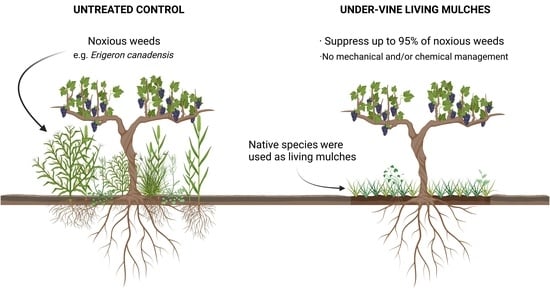
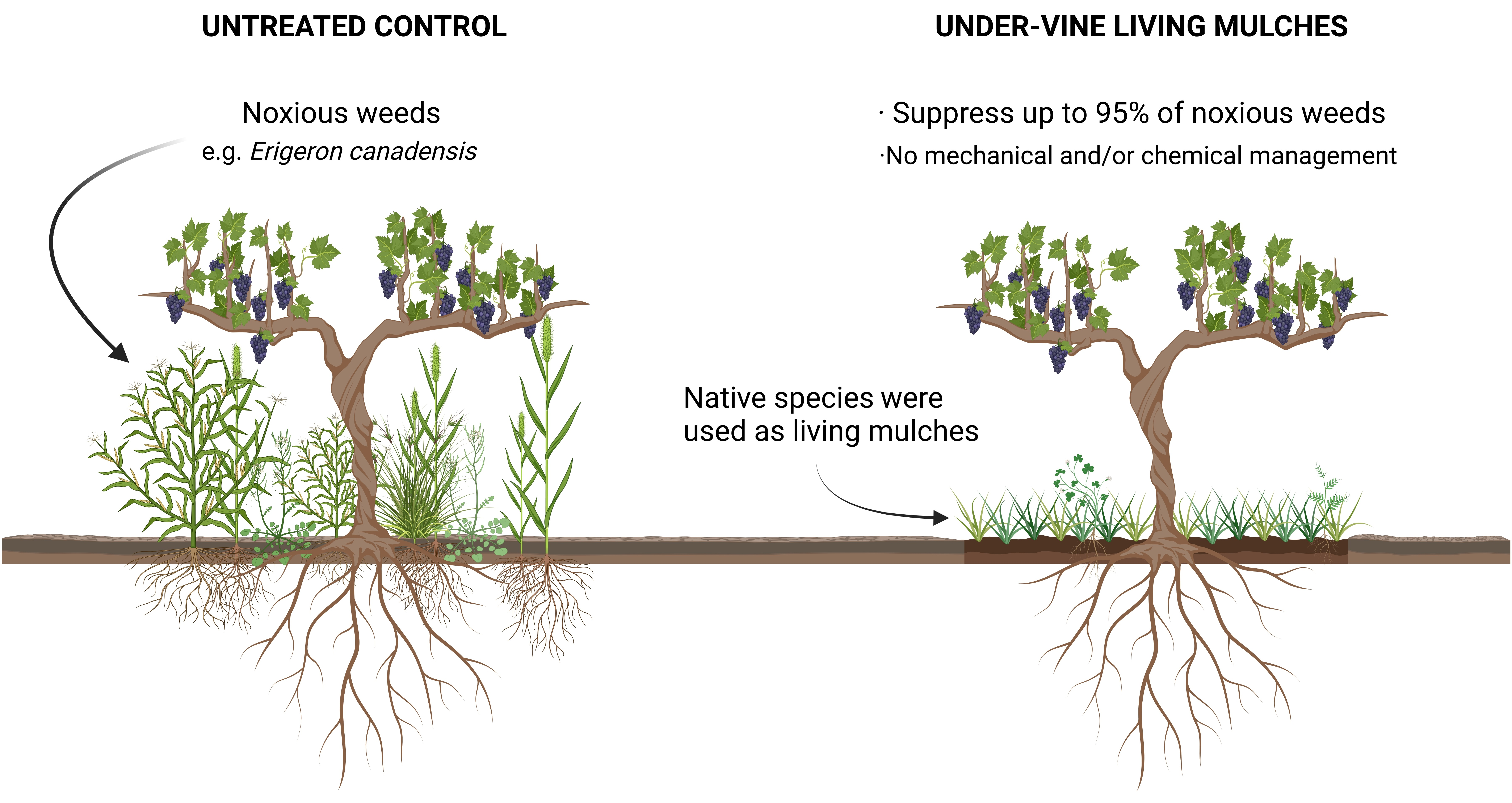
Use of Under-Vine Living Mulches to Control Noxious Weeds in Irrigated Mediterranean Vineyards

Abstract

This article assesses the use of under-vine living mulches in Mediterranean vineyards characterized by limited water resources, one of the reasons why this agronomic practice is currently unusual in these environments. The aim of the study was to test whether the use of this alternative method in Mediterranean vineyards could suppress noxious weeds without hindering optimal vineyard development. For this purpose, four native species were selected as living mulches: Festuca ovina, Pilosella officinarum, Plantago coronopus, and Plantago lanceolata. The variables measured during three years in two different experimental farms were: (a) living mulch cover, as a possible predictor of weed suppression success; (b) weed density and weed biomass, with special attention to noxious weed species; and (c) pruning weights, measured in the last year to analyze the cumulative effect of the treatments on the grapevine vegetative growth. Our results revealed that living mulches with high cover rates (average over 70%) also showed weed suppression of up to 95%, significantly controlling the occurrence of noxious weeds such as Erigeron canadensis. No significant effect of the different treatments on vine vegetative growth was found, although further studies would be necessary. Based on these findings, it can be concluded that under-vine living mulches could be an efficient and environmentally friendly method for weed control in Mediterranean vineyards where irrigation is available.

1. Introduction

Vineyards are one of the essential crops of the Mediterranean basin, where they have occupied a central role in the landscape, culture, and economy since ancient times [1]. Indeed, Spain (961 kha), France (797 kha), and Italy (719 kha) account for 34% of the world’s vineyard area [2]. Although traditionally, vineyards have been cultivated under rainfed conditions, in recent decades, the use of irrigation has become widespread in Mediterranean vineyards [3]. In the context of climate change, given the predictions of reduced rainfall in the Mediterranean basin [4], the area occupied by irrigated vineyards is expected to increase. Although this could prevent the detrimental effects of water shortage on vineyard yields [5], it could also have other undesirable effects, such as an increase in the presence of competitive and noxious weed species [6,7]. Winegrowers have tried to eradicate weeds in vineyards through conventional management based on the recurrent application of mechanical (tillage) and/or chemical (herbicides) control methods. However, numerous studies have highlighted in recent years critical problems associated with these weed management practices, such as the emergence of herbicide-resistant species [8], soil erosion [9], or biodiversity decline [7]. This has led to a search for alternative weed management in line with the European Green Deal (EU Farm to Fork Strategy), being the use of plant covers (e.g., cover crops, spontaneous plant covers) as one of the main alternatives to conventional management. Plant covers can provide multiple ecosystem services, such as erosion reduction, increased populations of natural enemies of crop pests, or biodiversity enhancement [7,10,11,12,13], but can also have a depressive effect on grapevine vigor and vineyard yield [7,14,15], therefore, some precautions would be necessary when used in Mediterranean vineyards. Nonetheless, winegrowers are looking for a balance in vegetative growth since excessive vine growth can have negative effects in terms of reduced fruit and wine quality [16,17].

In the case of cover crops (i.e., sown plant covers), one of the main benefits widely reported is weed control [18,19,20,21], which can be strongly correlated with cover crop biomass and cover crop type. Thus, cover crop biomass is inversely related to weed biomass and weed density [22], with grasses in general providing greater weed suppression than broadleaf species [21,22]. A particular case within cover crops are living mulches, which are maintained alive throughout the crop growing season [23], usually consisting of perennial plants that form a permanent cover without requiring annual seeding [24]. The usual purpose of living mulch application has typically been weed control [25,26,27,28], being more frequent in woody crop rows, where they could provide effective weed control but not significantly affect crop yields [24]. Living mulches have been tested for years on arable and woody crops, with positive effects on soil quality [29,30,31], beneficial insects [32,33], or soil organic carbon [34,35]. Some experiments with under-vine living mulches have been documented in humid-climate vineyards, revealing, beyond the benefits mentioned above, their usefulness in controlling grapevine vigor and achieving a more balanced vegetative growth [36,37,38,39]. However, in Mediterranean climates where vineyard-producing areas are generally associated with a scarcity of water resources, their use is still very unusual [40] and plant covers, if any, are commonly limited to the vineyard inter-rows. Nonetheless, combining under-vine living mulches with irrigation application could be a suitable strategy, as plant covers, besides improving soil conditions and water infiltration, could also limit the presence of noxious weed species [7,41]; while irrigation application could reduce the negative impact of water competition due to plant covers on the vineyard [42]. Therefore, such competition between cover crops and grapevines must be carefully managed to avoid undesirable results in grape production and quality [43].

With the main objective of assessing the influence of permanent plant covers along vineyard rows on noxious weed populations as well as on vineyard growth development, a study was carried out from 2018 to 2021 in two irrigated Mediterranean vineyards using four herbaceous species as under-vine living mulches (Festuca ovina, Pilosella officinarum, Plantago coronopus, and Plantago lanceolata). We hypothesized that a permanent plant cover without specific management needs could limit the presence of noxious weeds, while not limiting the development of vines. To this end, after the experiments were implemented in 2018, in the following years, we analyzed the effect of the four living mulches on weed density and weed biomass, particularly on the suppression of noxious weed species. In addition, the effect of the different living mulches on grapevine vegetative growth was also measured. The results provided here could help to extend this alternative weed management method to other Mediterranean vineyards.

2. Materials and Methods

2.1. Study Site

The study was conducted in parallel in two experimental vineyards located in a wine-growing region in the center of the Iberian Peninsula: (A) ICA-CSIC farm “La Poveda” (Arganda del Rey, Madrid, Spain; altitude 613 m.a.s.l.); and (B) IMIDRA farm “El Socorro” (Colmenar de Oreja, Madrid, Spain; altitude 755 m.a.s.l.). The climate in the region is semi-arid continental Mediterranean, with a mean annual temperature in “La Poveda” of 15.1 °C and average annual rainfall of 369 mm, while 13.7 °C and 421 mm in “El Socorro” (data from local neighboring weather stations for the period 2001–2021). Detailed climate data for the study period are shown in

Table 1. Mean temperature (T_mean) and cumulative rainfall (R) on the two experimental farms (La Poveda, farm A; El Socorro, farm B) during the study period, grouped in two intervals: the summer season (June to September) and the rest of the year (October to May). The percentage variation of accumulated precipitation (ΔR) in each time interval with respect to the average precipitation value (data for the period 2001–2021) for the same interval is also indicated.

	Farm A			Farm B
	Tmean (°C)	R (mm)	ΔR (%)	Tmean (°C)	R (mm)	ΔR (%)
October 2018–May 2019	11.2	172.0	−45	9.7	240.4	−33
June–September 2019	24.8	150.0	177	22.4	68.6	11
October 2019–May 2020	12.2	318.4	1	10.3	424.4	18
June–September 2020	24.3	21.0	−61	22.0	73.2	19
October 2020–May 2021	11.0	220.6	−30	9.4	286.2	−20
June–September 2021	24.2	123.6	129	21.9	149.4	142

. The soil type is Xerofluvent (pH 8.1) with a sandy loam texture in “La Poveda” and Calcic Haploxeralf (pH 8.4) with a clay loam texture in “El Socorro”. Grapevines (Vitis vinifera L. cv. Tempranillo) were grown in both fields in the Cordon Royat formation, with a planting frame of 2.5 m (inter-row spacing) × 1.2 m (inter-vine spacing) in “La Poveda”, while 2 m × 1.1 m in “El Socorro”. The vineyard inter-rows were tilled with cultivator in “La Poveda”, while mowed with a flail mower in “El Socorro”. On both farms, deficit drip irrigation was applied in the vineyard rows from May to September.

2.2. Plant Species Selected for Living Mulches

The key premise was to seek species that could permanently cover the soil without the need for reseeding. Thus, after an initial screening (apart from the four species chosen for this study, Astragalus hamosus L., Lotus corniculatus L., Medicago polymorpha L., and Sulla coronaria (L.) B.H.Choi & H.Ohashi were assessed), four indigenous species that are common in the Mediterranean flora were selected: Festuca ovina L., Pilosella officinarum Vaill., Plantago coronopus L., and Plantago lanceolata L. These species were chosen on the basis of their different functional traits to assess their ability to compete with other species and form monospecific covers (

Table 2. Traits of the plant species used as living mulches. Trait data have been compiled from FAWC Database [6]. Biomass estimation is described in Appendix A. RLF, Raunkiær life form; PHV, plant height (vegetative); LA, leaf area; LM, leaf mass; LDMC, leaf dry matter content, SLA, specific leaf area; CSR, plant CSR strategy according to Hodgson et al. [51].

	EPPO Code	Biomass	RLF	PHV	LA	LM	LDMC	SLA	CSR
		(g m−2)	-	(cm)	(mm2)	(g)	(mg g−1)	(mm2 mg−1)	-
Festuca ovina	FESOV	1083.2	H	17.1	46.7	1.9	422.1	14.0	S/CSR
Pilosella officinarum	HIEPI	256.8	H	7.3	258.8	18.9	207.0	16.0	S/CSR
Plantago coronopus	PLACO	491.3	H/Th	10.2	195.9	13.4	124.8	18.3	SR/CSR
Plantago lanceoalata	PLALA	1102.8	H	18.3	1653.3	95.4	178.6	18.9	SC/CSR

). Festuca ovina is a tuft-forming perennial grass previously used as under-vine plant cover [36], which forms a dense grass cover that could intercept weed seed rain, as described by Doisy et al. [44]. Pilosella officinarum is a prostrate growing plant with sexual, apomictic, and vegetative (by stolons) reproduction [45,46], which has a high colonizing potential as it is able to rapidly form monospecific patches and exclude other species [47], being considered a potentially invasive species in grasslands outside its natural range [48,49]. Plantago coronopus is a biennial (rarely perennial) rosette plant, while Plantago lanceolata is a perennial rosette species that has already been used in cover crop mixtures in vineyards [50]. Both Plantago species could control weed emergence by competing effectively for light and nutrients [20,23], with this competition expected to be greater in Plantago lanceolata, given its higher biomass. Nonetheless, their competitive ability may be conditioned by their different life cycles, i.e., perennials vs. biennials.

2.3. Experimental Design

The experimental design consisted of randomized blocks with four replications and six treatments: (i) an untreated control (UC); (ii) a weed-free control by manual weeding (WC) to estimate the vineyard growth development in the absence of weeds; and four under-vine living mulches, (iii) Festuca ovina (FO), (iv) Pilosella officinarum (PO), (v) Plantago coronopus (PC), and (vi) Plantago lanceolata (PL). Each treatment was distributed along eight inter-vine spacing, i.e., 9.6 m in La Poveda (8 × 1.2 m) and 8.8 m in El Socorro (8 × 1.1 m). The four selected species were planted in autumn 2018, in a strip 0.5 m wide under the vineyard row. With the exception of Pilosella officinarum, which was transplanted (density of 12 plants regularly distributed in the inter-vine spacing) from vegetative material collected from a nearby population, the rest of the species were sown from seed (seeding rates following the recommendations of the seed supplier: Festuca ovina, 9.5 g m⁻²; Plantago coronopus, 1 g m⁻²; Plantago lanceolata, 2 g m⁻²).

2.4. Field Data Collection

After the year of establishment, in the following three years (i.e., from 2019 to 2021) plant surveys were conducted at two different times, coinciding with the early and late crop growing season (May and September, respectively), by placing three sampling frames (0.33 × 0.33 m) in each of the 40 plots (2 fields × 4 replications × 5 treatments, excluding the weed-free control). At each sampling frame, the percentage cover of target species used as living mulch was estimated [52].

Previous studies in non-permanent cover crops have commonly used cover crop biomass as a predictor of weed suppression effect [22,53,54]. In our case, being a permanent cover crop, a non-destructive method was chosen in order not to affect plant viability, so the percentage cover of living mulches was measured as a possible predictor of weed suppression. Additionally, a rough estimation of living mulches biomass was made, as explained in Appendix A, in order to compare our results with previous studies.

Weed species (in a broad sense, all spontaneous flora) were identified from Castroviejo [55], updating the nomenclature according to International Plant Names Index [56], and weed density (number of individuals per m²) was recorded. All weeds at each sampling frame were collected in paper bags, dried in the laboratory (oven at 105 °C for 24 h) and weighed on a precision balance to obtain the weed biomass data.

Finally, the cumulative effect of the three years of treatments on grapevine vegetative growth was estimated. For this purpose, the pruning weights of the six central vines in each plot (i.e., excluding border vines) in each of the 48 plots (2 fields × 4 replications × 6 treatments, including the weed-free control) were measured in the last year (i.e., 2021).

2.5. Statistical Analysis

The effect of the treatments on the response variables was measured separately for each experimental farm using independent models because of contrasting differences (i.e., soil type, weather, etc.) between the two farms. On the one hand, the degree of establishment of different species used as under-vine living mulches was analyzed, using the vegetation cover as the response variable, treatment (FO, PO, PC, PL), and year as the fixed factors. Year was used as a fixed effect since the temporal evolution of living mulches could follow a non-random pattern specific to each species. Living mulches vegetation cover was expressed as a decimal (i.e., range 0 to 1) to fit a generalized linear model with beta distribution [57].

On the other hand, weed data were pooled from the three sampling frames per plot, thereby obtaining a matrix that included data per plot for two sampling times and for three years (40 plots × 2 sampling times × 3 years; n = 240). Weed density models were constructed for overall species and, individually, for those species with a significant presence. To determine which species had significant presence, the absolute weed density data were transformed into relative density:

$$\mathrm{Relative} \mathrm{density}=\frac{\mathrm{number} \mathrm{of} \mathrm{individuals} \mathrm{of} \mathrm{a} \mathrm{species} \mathrm{on} \mathrm{a} \mathrm{plot} x}{\mathrm{total} \mathrm{number} \mathrm{of} \mathrm{individuals} \mathrm{on} \mathrm{plot} x}\times 100$$

A significant presence was thus established in this work for those species with relative density >3%. The effect of the different treatments (UC, FO, PO, PC, PL) on weed density and weed biomass was estimated using generalized linear mixed models, fitted with a negative binomial distribution for weed density and a gamma distribution for weed biomass. In total weed density and weed biomass models, the year was used as a fixed effect, considering that both total density and biomass of species depend on living mulches cover, which in turn depends on the year factor. However, in the individual species density models, the year was considered a random effect since the higher or lower density of a species can be driven by stochastic processes. In general, block was used as a random effect. The relationship of weed density and weed biomass (response variables) with living mulches cover was explored using linear regression models and Spearman’s correlation test. In the same way, the relationship between living mulch cover and the ratio weed biomass/density was analyzed. The lower this ratio, the lower the average biomass of weeds present in a plot. This correlation could provide an analysis of whether weed biomass per plant unit increases or decreases as a function of living mulch cover.

Additionally, a linear mixed model was constructed to measure the effect of the different treatments (WC, UC, FO, PO, PC, PL) on grapevine vegetative growth, including block as a random effect. A logarithmic transformation (log[x + 1]) was performed to fit the response variable to a normal distribution. The relationship between grapevine vegetative growth and weed biomass was measured using a Spearman correlation test.

All statistical analyses were performed in R 4.1.0. Beta regression models were fitted with the betareg package in R [58], estimating its fit by pseudo R². Generalized linear mixed models were fitted with the GLMMtmb package [59], computing marginal R² (fixed effects variance) and conditional R² (full model variance) using the performance package [60]. The corrected Akaike Information Criterion (AICc) was applied to screen the best models, selecting those with the lowest AICc score. For all models, the statistical significance of the fixed effects was estimated by a type III ANOVA test. To compare the mean of the levels of one factor, the Student’s t-test was performed, adjusting the p-values with the Bonferroni correction.

3. Results

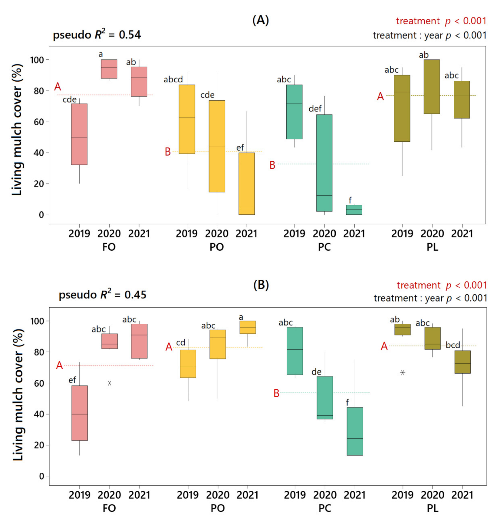
3.1. Establishment of Under-Vine Living Mulches

The percentage cover observed in living mulches varied according to the species used, the year and the farm studied (Figure 1). Living mulches of Festuca ovina and Plantago lanceolata (hereinafter, FO living mulch and PL living mulch) were successfully established on the two farms studied, showing an average cover (over the three years) of about 80% on both farms. In the case of FO living mulch, although in the first year the percentage of cover barely exceeded 40%, from the second year onwards, it reached cover close to 100%. Regarding PL living mulch, no significant inter-annual variations were found, although a decrease in the percentage cover was observed in the third year. The living mulch of Plantago coronopus (hereinafter, PC living mulch) was successfully established in the first year but showed a drastic decrease in the percentage cover from the second year onwards, thus registering in the whole three years and the two farms with the lowest establishment values compared to the other living mulches. In the case of living mulch of Pilosella officinarum (hereinafter, PO living mulch), the observed response was clearly different between farms. On farm “La Poveda” (hereinafter, farm A), although in the first year the percentage cover did not differ significantly from that observed for the other species, from the second year onwards, a decline began, which was significantly marked in the third year, when in some plots the percentage cover dropped below 10%. In contrast, the percentage cover of PO living mulch on farm “El Socorro” (hereinafter, farm B) increased over the years, from 68% to 95% average cover from 2019 to 2021, respectively.

3.2. Effect of Under-Vine Living Mulches on Weed Density

A total of 59 plant species were identified during the three years of weed sampling, 35 on farm A and 42 on farm B, of which 18 species were present on both farms (

Table 3. List of weeds present on the two study farms during the two sampling dates, May and September (average of the three years 2019 to 2021), ranked in order of highest to lowest relative density. Those species classified as noxious weeds are indicated with an asterisk next to the EPPO code. The + and – signs indicate that the relative density of the species was less than 0.01% (+) or that the species was not found (−).

EPPO Code	Scientific Name	Farm A		Farm B
		May	September	May	September
EPHCH	Euphorbia prostrata Aiton	0.01	0.02	0.25	0.71
ERICA *	Erigeron canadensis L.	0.43	0.35	−	−
BROMA	Bromus madritensis L.	0.20	0.07	0.11	0.04
CONAR *	Convolvulus arvensis L.	0.01	0.01	0.11	0.14
CYPRO *	Cyperus rotundus L.	0.05	0.17	−	−
FESAR	Lolium arundinaceum (Schreb.) Darbysh.	−	0.21	−	−
SONAS *	Sonchus asper (L.) Hill	0.06	0.01	0.11	0.03
GALPR	Galium parisiense L.	0.01	−	0.13	−
CYNDA *	Cynodon dactylon (L.) Pers.	0.05	0.06	−	−
DIPER *	Diplotaxis erucoides (L.) DC.	−	−	0.07	0.03
MEDMI	Medicago minima (L.) Bartal.	−	+	0.09	+
CHEAL *	Chenopodium album L.	0.03	0.03	−	−
BRODI *	Bromus diandrus Roth	0.04	−	0.01	−
LACSE*	Lactuca serriola L.	0.01	+	0.02	0.01
SOLNI *	Solanum nigrum L.	0.02	0.02	−	+
SETVI	Setaria viridis (L.) P.Beauv.	0.02	0.01	−	−
ANGAR	Lysimachia arvensis (L.) U.Manns & Anderb.	0.01	0.01	−	−
POLAV	Polygonum aviculare L.	+	+	−	0.02
LOLRI	Lolium rigidum Gaudin	0.02	−	0.01	−
SONOL *	Sonchus oleraceus L.	+	−	+	−
HORMU	Hordeum murinum L.	+	−	0.02	−
MEDOR	Medicago orbicularis (L.) Bartal.	-	−	0.02	−
ASAHA	Astragalus hamosus L.	+	−	0.01	−
CIRAR *	Cirsium arvense (L.) Scop.	−	−	+	0.01
AMAAL *	Amaranthus albus L.	+	+	+	+
POROL	Portulaca oleracea L.	−	0.01	−	−
SASKA *	Salsola kali L.	+	+	−	+
AVEST	Avena sterilis L.	−	−	0.01	−
ECHCG	Echinochloa crus-galli (L.) P.Beauv.	−	+	−	−
BROTE	Bromus tectorum L.	−	−	+	−
FILPY	Filago pyramidata L.	−	−	+	−
PAPRH	Papaver rhoeas L.	+	+	−	+
LPHCR	Rostraria cristata (L.) Tzvelev	+	−	+	−
MALSI *	Malva sylvestris L.	−	−	+	+
TRKMO	Medicago monspeliaca (L.) Trautv.	−	−	+	−
VEBOF	Verbena officinalis L.	−	−	+	−
VLPMY	Festuca myuros L.	−	−	+	−
HEOEU	Heliotropium europaeum L.	+	+	−	−
GERMO	Geranium molle L.	−	−	+	+
FUMOF	Fumaria officinalis L.	+	−	−	−
VERHE	Veronica hederifolia L.	+	−	−	−
CENME	Centaurea melitensis L.	−	−	+	−
CVPVT	Crepis vesicaria subsp. taraxacifolia (Thuill.) Thell.	−	−	+	−
LAMAM	Lamium amplexicaule L.	−	−	+	−
SCVLA	Scorzonera laciniata L.	−	−	+	−
TROPS	Tragopogon porrifolius L.	−	−	+	−
ASAST	Astragalus stella L.	−	−	+	−
BRORU	Bromus rubens L.	−	−	+	−
ERXCA	Eryngium campestre L.	−	−	+	−
HESCO	Sulla coronaria (L.) B.H.Choi & H.Ohashi	−	−	+	−
TANCR	Taeniatherum caput-medusae (L.) Nevski	−	−	+	−
TAROV	Taraxacum obovatum (Willd.) DC.	−	−	+	−
CAPBP	Capsella bursa-pastoris (L.) Medik.	+	−	−	−
PLAMA	Plantago major L.	+	−	−	−
PLAOV	Plantago ovata Forssk.	+	−	−	−
RBITI *	Rubia tinctorum L.	+	−	−	−
TRBTE	Tribulus terrestris L.	−	+	−	−
HEQGL	Herniaria glabra L.	−	−	+	−
MEDRI	Medicago rigidula (L.) All.	−	−	+	−

). On farm A, the most abundant species were Erigeron canadensis (relative density of 39%), Bromus madritensis (13%), Cyperus rotundus (12%), and Lolium arundinaceum (12%). Weed community composition was different on farm B, with Euphorbia prostrata (52%), Convolvulus arvensis (13%), B. madritensis (7%), and Sonchus asper (6%) as the most abundant species.

The use of living mulches had a significant effect on weed density, although the effect varied depending on the mulching species used and the weed species to be controlled. On farm A, FO and PL living mulches drastically reduced total weed density compared to the control, and a smaller but significant reduction in PC living mulch was observed (Figure 2). On farm B, only the two Plantago species showed a significant reduction in total weed density, with the suppression by PL living mulch being particularly marked.

When the year factor was considered (i.e., treatment: year), different patterns were shown according to the living mulch species (Figure 2). For example, a regular behavior in all three years, either because showing significant differences with respect to untreated control (hereinafter UC), e.g., in PL living mulch on both farms and FO living mulch on farm A, or because showing no significant differences with respect to UC, e.g., in PO living mulch on farm A. However, other remarkable patterns were found in species such as PC living mulch, which showed a significant reduction in weed density only during the first two years, then losing this weed-suppressive capacity in the third year on both farms. An opposite pattern was observed in FO living mulch on farm B, since during the first year had no effect on weeds (UC = 279 plants m⁻²; FO = 308 plants m⁻²), but from the second year onwards, drastically reduced the total weed density.

The effect of living mulches on the density of weed species with a significant presence (i.e., relative density > 3%) is shown in

Table 4. Effect of treatments on the density of weeds with a significant occurrence (relative density > 3%). Those species classified as noxious weeds are indicated with an asterisk next to the EPPO code. The percentage of variation in weed density that is explained by the fixed effects of the model is indicated (R²_m). A type III ANOVA was used to calculate the significance level of the effect (p-values: *** p < 0.001, ** p < 0.01, * p < 0.05, ns not significant), followed by a t-test adjusted with a Bonferroni correction for pairwise comparison. For each farm, treatment means sharing the same letter within each row are not significantly different.

	Farm A							Farm B
	R2m	p-Value	UC	FO	PO	PC	PL	R2m	p-Value	UC	FO	PO	PC	PL
BROMA	0.40	***	33.67 a	1.53 b	27.17 ab	17.98 ab	1.53 b	0.32	***	17.98 a	3.44 b	9.18 ab	3.83 b	0.77 b
CHEAL *	0.09	ns	1.53 a	0.38 a	10.33 a	4.97 a	2.30 a	−	−	−	−	−	−	−
CONAR *	−	−	−	−	−	−	−	0.20	***	16.45 a	13.39 ab	12.63 ab	17.60 a	4.59 b
CYNDA *	0.16	***	4.21 b	0.77 b	21.04 a	3.83 b	6.89 ab	−	−	−	−	−	−	−
CYPRO *	0.34	**	14.54 ab	2.68 b	22.96 ab	30.61 a	0.38 b	−	−	−	−	−	−	−
DIPER *	−	−	−	−	−	−	−	0.02	ns	3.44 a	9.18 a	3.83 a	4.97 a	4.59 a
EPHCH	−	−	−	−	−	−	−	0.07	***	81.11 a	77.67 a	61.98 ab	32.52 ab	10.33 b
ERICA *	0.42	***	128.18 a	10.71 c	66.57 b	36.35 bc	3.44 c	−	−	−	−	−	−	−
FESAR	0.06	ns	30.23 a	9.57 a	26.78 a	4.21 a	1.91 a	−	−	−	−	−	−	−
GALPR	−	−	−	−	−	−	−	0.34	**	16.45 a	1.53 b	7.65 ab	1.91 b	0.00 b
MEDMI	−	−	−	−	−	−	−	0.35	*	7.27 a	6.50 a	2.68 ab	1.53 ab	0.00 b
SONAS *	0.26	**	8.80 a	0.77 b	8.80 a	3.06 ab	0.38 b	0.43	***	10.71 a	7.65 ab	3.83 bc	3.83 bc	1.15 c

. On farm A, the four living mulches significantly reduced the presence of the noxious weed E. canadensis (ERICA), especially FO and PL living mulches, with weed suppression of 92% and 97%, respectively. The density of S. asper (SONAS) was significantly reduced by PL living mulch on both farms, by FO living mulch on farm A, and by PO and PC living mulches on farm B. Noxious weed C. arvensis (CONAR) was also significantly suppressed by PL living mulch on farm B.

Beyond the effect on noxious weeds, FO and PL living mulches significantly reduced the density of B. madritensis (BROMA) on both farms. In addition, PL living mulch significantly reduced the occurrence of the most abundant species on farm B, Euphorbia prostrata (EPHCH).

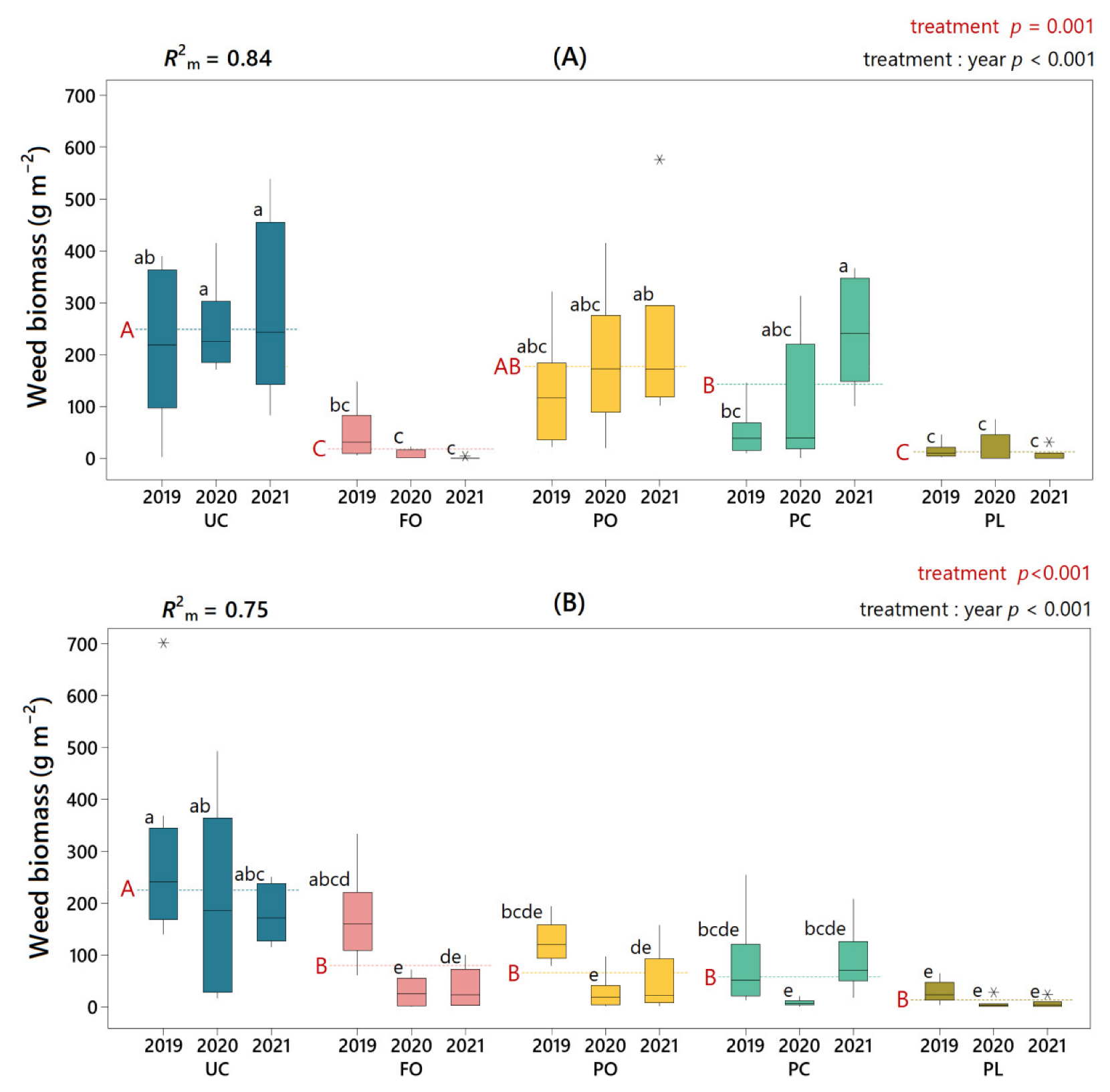
3.3. Effect of Under-Vine Living Mulches on Weed Biomass

Similar to that observed for weed density, the results of this study have shown how the use of different living mulches largely explains the observed variance in weed biomass in both farm A (R²_m = 0.84) and farm B (R²_m = 0.75) (Figure 3). Considering the three-year average, FO and Plantago (i.e., both PC and PL) living mulches significantly reduced weed biomass on farm A compared to the control, with an average reduction of 95% for PL living mulch (UC = 248.64 g m⁻²; PL = 12.25 g m⁻²) and 93% for FO (UC = 248.64 g m⁻²; FO = 18.07 g m⁻²). On farm B, a significant reduction was observed for all four mulching species, particularly in PL living mulch, which showed a 93% reduction in weed biomass compared to the control (UC = 204.59 g m⁻²; PL = 13.73 g m⁻²).

The analysis accounting for the year factor (i.e., treatment: year) showed that weed biomass reduction by FO living mulch on both farms was not statistically significant in the first year but was significant in the following two years. Regarding PC living mulch, weed biomass reduction was only significant in the first two years on farm B. Regular patterns throughout the years were found for the other two species used as living mulches, with significant differences with respect to UC in PL on both farms and PO on farm B, while no significant differences in PO on farm A.

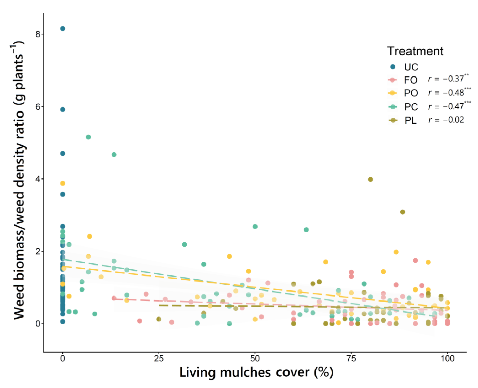
3.4. Relationships between Living Mulch Cover, Weed Density and Weed Biomass

Overall, negative correlations were observed between living mulch cover and weed density and weed biomass, being clearly stronger on farm A than farm B and more robust when weed biomass was considered as a response variable (

Table 5. Correlations between living mulch cover and weed density and weed biomass, calculated for the two farms (overall) and for each farm separately. The correlation value (r) was estimated using a Spearman correlation test. The significance level of the correlations is also indicated (*** p < 0.001).

	Overall
	Weed density	Weed biomass
Living mulch cover	−0.60 ***	−0.69 ***
	Farm A
	Weed density	Weed biomass
Living mulch cover	−0.72 ***	−0.79 ***
	Farm B
	Weed density	Weed biomass
Living mulch cover	−0.45 ***	−0.57 ***

). These relationships were consistent as a similar response was observed on both farms. Indeed, a strong negative correlation was observed between living mulch cover and weed biomass in both farm A (r = −0.79) and farm B (r = −0.57), which exhibited a better fit using a quadratic regression models, where the slope of the curve flattens out at cover percentages above 75% (Figure 4A). However, a different response depending on the type of living mulch was found when studying the relationship between weed biomass and living mulch cover (Figure 4B).

While FO and PO living mulch covers were strongly correlated with weed biomass, this relationship was weaker in the two Plantago species, especially in PL living mulch, where the observed correlation was not even significant. These differentiated responses therefore conditioned the average weed suppression reached by each living mulch. For example, PC living mulch resulted in high weed suppression (71%) with intermediate levels of cover (54%) on farm B, while PO living mulch required much higher cover (83%) to reach a similar level of suppression (68%) (

Table 6. Summary table showing for each living mulch (FO, Festuca ovina; PO, Pilosella officinarum; PC, Plantago coronopus, and PL, Plantago lanceolata) the average living mulch cover, weed suppression percentage and weed biomass/weed density ratio.

	Farm A			Farm B
	Living Mulch Cover (%)	Weed Supression (%) a	Ratio (g Plants−1) b	Living Mulch Cover (%)	Weed Supression (%) a	Ratio (g Plants−1) b
FO	77	93	0.31	71	61	0.61
PO	41	29	1.01	83	68	0.71
PC	33	43	1.17	54	71	0.97
PL	77	95	0.40	84	93	0.51

^a Weed biomass reduction of the living mulch with respect to the control expressed as a percentage. ^b Ratio of weed biomass to weed density (i.e., how much weed biomass there is per weed).

). When the correlation between living mulch cover and the ratio weed biomass/weed density was analyzed, contrasting responses were also observed according to the type of living mulch (Figure 5). In this case, it was the FO and PL living mulches that showed a weaker correlation, exhibiting, on average, a markedly lower ratio than that observed for PO and PC living mulches (Table 6).

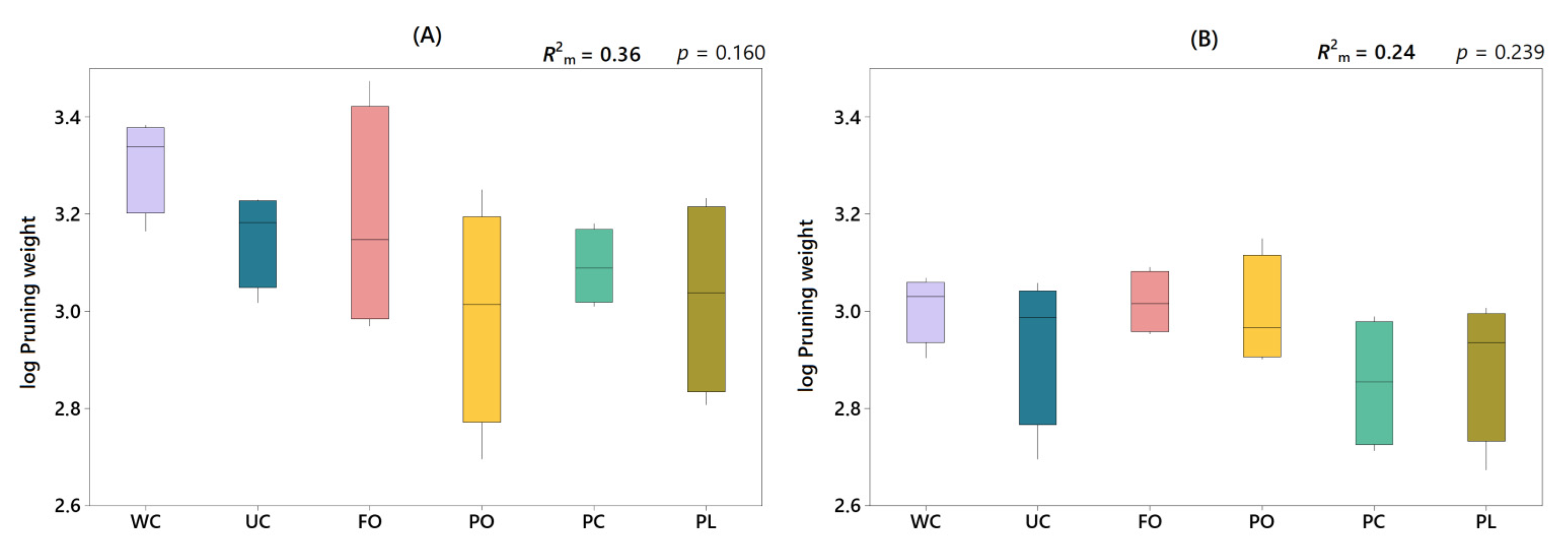
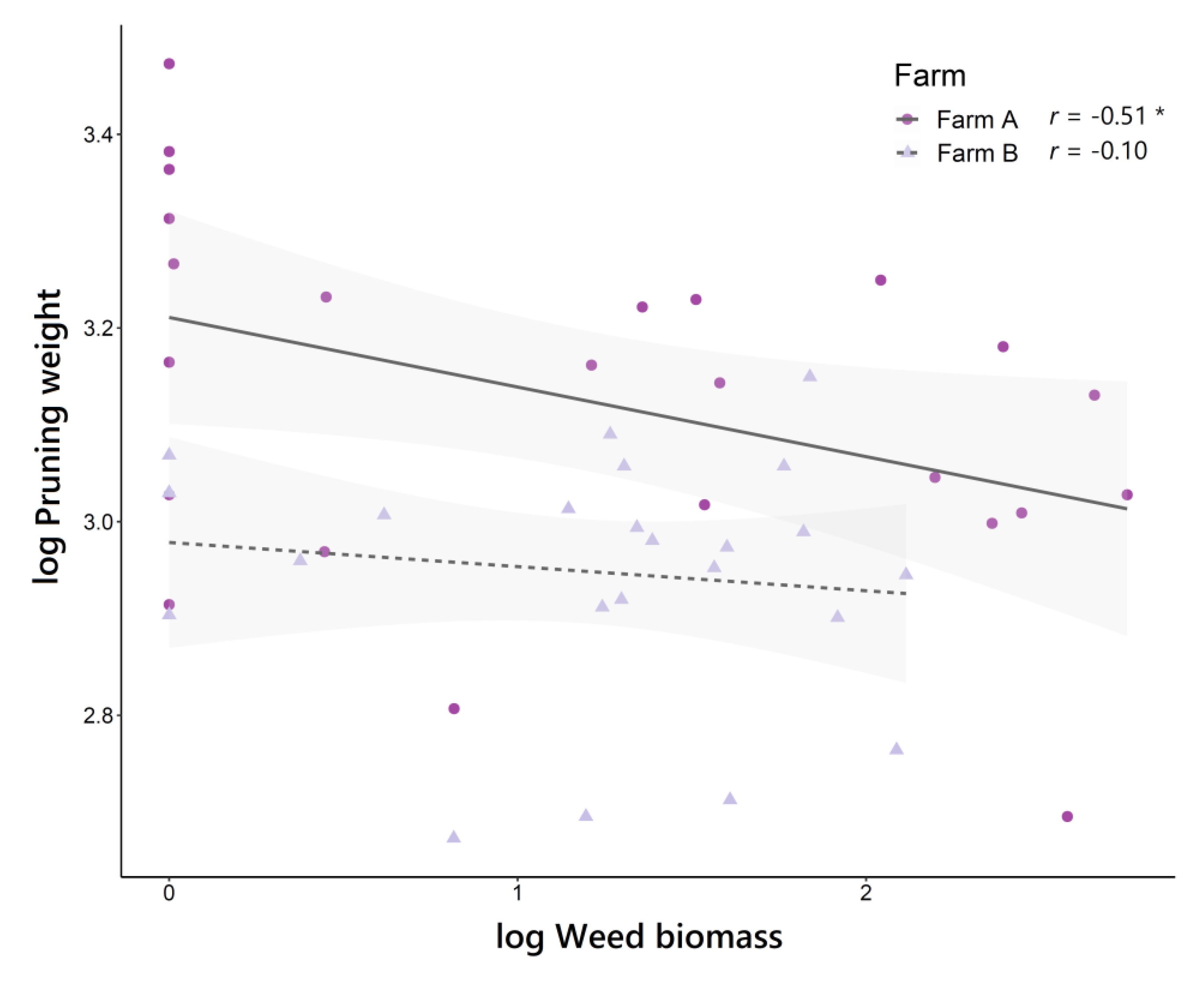
3.5. Effect of Under-Vine Living Mulches on Grapevine Vegetative Growth

The different treatments applied explained part of the variance observed in grapevine vegetative growth (based on pruning weights), both on farm A (R²_m = 0.36) and farm B (R²_m = 0.24) (Figure 6). However, although a slight reduction in pruning weights was observed in living mulches compared to weed-free control (WC) on both farms, there were no significant differences between treatments. An analysis of the relationship between grapevine vegetative growth and weed biomass showed a negative correlation between the two variables, with pruning weight being lower the higher the weed biomass (Figure 7). However, this correlation was only significant on farm A (r = −0.51*), while on farm B, it was clearly weaker (r = −0.10).

4. Discussion

4.1. Extend of Establishment of Under-Vine Living Mulches

Our results revealed that the living mulches with the most successful establishment were PL and FO living mulches on farm A, and PL and PO living mulches on farm B. In general, similar patterns of establishment were found in both farms for FO, PC, and PL living mulches, which suggests that they were more influenced by intrinsic traits of each species than by differential environmental factors of each farm. Indeed, FO living mulch had a limited establishment in the first year (50.9% on farm A, 41.1% on farm B), but in the second and third year they reached coverages above 80%, regardless of the farm. This is consistent with previous studies showing that Festuca ovina is a slow-growing species with slow establishment [61] and with a lower emergence rate than Plantago species used as living mulches [62]. On the other hand, the decrease in PC living mulch cover from the second year onwards probably occurred because Plantago coronopus is a biennial species; this study further found that spontaneous regeneration from self-seeding was very limited. Seedling recruitment of Plantago coronopus is strongly conditioned by rainfall [63,64], so low rainfall during the October 2020–May 2021 period (see Table 1) may have limited the recruitment of new seedlings on both farms. A lower recruitment was observed on farm A (21.4% less cover of PC living mulches than on farm B), which could be due to the lower rainfall received and a lower water retention capacity of the sandy loam soil in this farm. In contrast, the perennial species of the same genus Plantago lanceolata, showed a high cover on both farms during the three years of observations. On this basis, selecting perennial species as living mulch would seem more appropriate since they are able to achieve successful establishment without reliance on the success of seeding and recruitment, as these processes, in turn, depend on environmental conditions that are difficult to manage.

With regard to PO living mulches, contrasting differences were observed in the percentage of cover recorded on both farms (a 77.8% higher cover on farm B than on farm A in the last year). Pilosella officinarum is a drought-tolerant species that, however, does not seem to tolerate high temperatures [45]. In fact, in the Iberian Peninsula it is part of dry grasslands of cool environments, being mainly found in mountain areas [55]. The presence of a natural population of P. officinarum on farm B suggested that its establishment could be successful, at least on this farm, which was later confirmed in the results. Conversely, our hypothesis for farm A is that the higher temperatures reached in the summer period, more than 2 °C higher than on farm B (Table 1), could have limited their survival. Accordingly, under a global warming scenario, the use of PO living mulches in our latitudes should be limited to areas with cooler temperatures where the survival of P. officinarum is assured.

4.2. Weed Suppression by Under-Vine Living Mulches

This three-year study has shown that, as expected, successfully established living mulches (i.e., high percentage cover) generally showed high weed suppression, in accordance with previous studies on permanent living mulches [24]. The living mulch of Plantago lanceolata showed the highest suppression capacity, higher than in the grass living mulch Festuca ovina in both farms, which challenges the previous assumption that grass cover crops provide more suppression than broadleaf species [21,22]. This prior assumption may be true for broadleaf species commonly used as cover crops (i.e., brassicas, legumes) but should not be generalized. In addition, our results revealed that the extent of living mulch cover was a good predictor of weed suppression, being inversely related to weed density and biomass, regardless of the farm. This is in line with Steinmaus et al. [65], who found a similar relationship between living mulch cover and weed suppression. In light of this, our assumption is that the higher the percentage of soil covered by living mulches, the less surface area available for weeds to colonize, germinate, and establish. Nevertheless, the relationship between living mulch cover and weed biomass varied depending on the species used as living mulch (Figure 4B). Thus, the weed suppression success of PO and FO living mulches was highly dependent on the coverage achieved, but living mulches of Plantago were less cover-dependent, especially PL living mulch, for which no significant correlation was observed. As discussed below, these differences could be due to the different suppression mechanisms of each species. In the case of PO living mulch, the small growth habit of Pilosella officinarum may limit its ability to compete for light and generate a shading effect, a key feature for weed suppression [20,66,67]. Therefore, the success of this species in suppressing weeds depends to a large extent on achieving high percentages of cover, as any gap in this living mulch provides a good chance for weeds to establish and thrive. The living mulch of Festuca ovina was also strongly cover-dependent, showing high weed suppression at high cover levels. However, its slow establishment generating only moderate cover during the first year may compromise weed suppression in this year of implantation. Once established and due to the dense tufted cover that this species forms, we consider that it can be very effective in intercepting seed rain [44] and suppressing weeds by shading, thus limiting weed seed germination and weed seedling growth. In fact, the low ratio observed between weed biomass and density in FO living mulch (Table 6) may be indicative of this suppressive effect on seedling growth. Similarly, a very low ratio was also found in PL living mulch. Both species (i.e., Festuca ovina and Plantago lanceolata) showed similar biomass and height, clearly higher than the other two species used (see Table 2). These traits could be considered a differential factor in terms of increased competition for light (the aforementioned “shading effect”) and nutrients against weeds, in line with previous work indicating that cover crop biomass is a key driver of weed suppression [22,53,54]. However, all the above does not explain why PL living mulch, with a biomass similar to that of FO living mulch, showed a higher weed suppression capacity compared to other living mulches even at intermediate cover levels (Figure 4B). A plausible explanation could lie in a physical mechanism associated with leaf traits, whereby the leaves of Plantago lanceolata, with a significantly larger leaf area than the others (Table 2), could shade a greater soil surface, therefore, a medium cover would be enough to exert a competitive shading. On the other hand, the presence of phytotoxic compounds has been cited in Plantago lanceolata [68] and other species of the genus [69], so that weed suppression could be partly related to allelopathic effects, although this could not be demonstrated in our study. In this sense, a lower relationship between weed biomass and leaf mass cover was observed in PC living mulch, achieving higher weed suppression than FO and PO living mulches at cover levels below 70% (Figure 4B). Given its growth habit and leaf size, we consider it unlikely that this is due to an increased shading effect, but possibly by an allelopathic effect.

4.3. Control of Noxious Weeds by Under-Vine Living Mulches

Our results indicated that the use of under-vine living mulches can drastically limit the occurrence of E. canadensis, as well as other problematic weeds in vineyards, such as Convolvulus arvensis or S. asper (Table 2). Erigeron canadensis is a highly competitive weed that poses a serious threat, given its resistance to glyphosate [70,71] and its depressive effect on grapevine vegetative growth [72]. This species was significantly controlled by all living mulches, especially by FO and PL living mulches (92% and 97% suppression), similar to the suppression levels found by Pittman et al. [73] in cover crops mixtures. Considering that germination of E. canadensis is highly light-dependent [74,75], our assumption is that Festuca ovina and Plantago lanceolata, with the highest shading capacity, were also the most effective in suppressing this noxious weed. This is in line with Steinmaus et al. [65], who observed that the use of living mulches in a Californian vineyard achieved high weed suppression due to light interception. In addition, Doisy et al. [44] have reported that grass covers (Festuca arundinacea Schreb and Dactylis glomerata L.) intercept 56% of seed rain of E. canadensis, which could likewise occur in FO living mulch. Similar effects of grass cover were reported on S. asper with 66% interception of seed rain [44], a species that also has a highly dependent germination on light received [74]. Therefore, as discussed for E. canadensis, we consider that these mechanisms could explain to a great extent the high suppression of S. asper by FO living mulch on farm A and by PL living mulch on both farms. The low suppression of S. asper by FO living mulch on farm B could be due, as discussed above, to the low establishment of F. ovina during the first year. This fact might also have limited the suppressive capacity of FO living mulch on C. arvensis, which was only significantly controlled by PL living mulch on farm B, with a 72% reduction with respect to control. This result is particularly relevant given that C. arvensis is a perennial geophyte, persistent and hard to manage, which can cause significant crop losses [76]. Our results contrast with the findings of Steinmaus et al. [65], as the living mulches used by them (Avena sativa L. and Vicia benghalensis L.) not only failed to control C. arvensis, but increased its dominance. Nonetheless, our results do not clarify the mechanism involved in the suppression of C. arvensis by PL living mulch, which could be due to a combination of all the mechanisms that have been discussed above.

Likewise, it should be noted that the two most abundant species in the vineyards studied were two invasive alien species: the aforementioned E. canadensis and Euphorbia prostrata, although the latter does not a priori pose any threat to grapevines. The application of irrigation in Mediterranean woody crops during the summer months can lead to the proliferation of alien weeds [77,78]. In the current context, in which the surface area occupied by irrigated vineyards in Mediterranean countries such as Spain is increasing exponentially [79], irrigated vineyard rows could be a potential reservoir of invasive alien weeds, some of which, such as E. canadensis or other species of the genus Erigeron, could be noxious grapevine weeds. Based on our results, the use of under-vine living mulches could be a successful option to avoid the proliferation of these species.

4.4. Effect of Under-Vine Living Mulches on Grapevine Vegetative Growth

Our results revealed no significant effect of the different treatments on grapevine vegetative growth, which contrasts with previous studies that observed a significant effect of under-vine living mulches on vegetative growth [37,38]. However, in these studies focusing on under-vine living mulches, the treatment is the same in both vineyard rows and inter-rows, similar to what Giese et al. [36] and Vanden Heuvel and Centinari [80] correctly referred to as “complete vineyard floor cover crops”. However, in other studies in which, like us, they applied the same management in vineyard inter-rows [39,40,81], they found no significant effect of the under-vine living mulches on vine vegetative growth. Notably, when under-vine living mulches are used in newly planted vineyards, a negative effect on vegetative growth can occur [82,83], even if the same management was applied in all vineyard inter-rows. Presumably, young vines with a less developed root system seem to be more susceptible to competition from plant cover [84]. Conversely, in studies contrasting different treatments in the vineyard rows (e.g., herbicides, tillage vs. cover crops) while keeping the same management on vineyard rows, a significant effect on pruning weights was found [42,43,85].

Considering the above, our assumption is that management of vineyard inter-rows (in our case, up to five times more area than the rows) could have a significant effect on grapevine vegetative growth, proportionally greater than the effect of management on the vineyard rows. Therefore, when management in the vineyard inter-rows is the same, homogeneous results of vegetative growth in mature vineyards are to be expected, regardless of the treatment applied in the vineyard rows. In this regard, although no significant differences were observed between treatments, farm A (with tilled inter-rows) showed, on average, greater pruning weights than farm B (with mown inter-rows). This is fully consistent with the results observed in a recent study on farm B [7], in which the authors found that the percentage of bare soil (considering both vineyard rows and inter-rows) is inversely related to vineyard yield, but also to grapevine vegetative growth (unpublished data). Thus, as in the present study, management with tilled inter-rows (higher percentage of bare soil) showed significantly higher pruning weights than management with mown inter-rows (lower percentage of bare soil).

On the other hand, our results also showed a slight negative correlation between weed biomass and grapevine vegetative growth, although it was only significant on farm A. For the above reasons, we assume that the effect of management on vineyard inter-rows attenuated any possible relationships between these two variables. Moreover, considering the higher weed biomass on farm A, associated with a high presence of the noxious weed E. canadensis, could justify the stronger correlation observed on farm A with respect to farm B, the latter with a clearly lower impact of weeds on the vegetative growth of the vineyard. Even so, the observed correlation supports the premise that control of weed biomass under vines may play a relative role in regulating grapevine vegetative growth.

4.5. Implications for Vineyard Weed Management

To our knowledge, under-vine living mulches have so far been a very unusual management in Mediterranean vineyards, being limited to experimental studies [40]. However, our study suggests that permanent under-vine living mulches can be successfully established in a semi-arid Mediterranean climate, suppressing noxious weeds without jeopardizing the grapevine vegetative growth. In conditions of water scarcity, it seems daring to consider keeping the whole vineyard surface (i.e., row and inter-row) with a permanent vegetation cover. Since the competition of plant cover with the vineyard will largely depend on the percentage of bare soil [7], and this percentage can be adapted according to soil properties to avoid competition for water [86], therefore a reasonable option would be to use permanent living mulches in irrigated vineyard rows, where there could be a higher occurrence of noxious grapevine weeds [7], and keeping free of vegetation the inter-row space through soil management that prevents competition with the vineyard as much as possible.

Finally, under-vine living mulches have a low establishment cost (see Appendix B) and, as has been demonstrated here, can suppress weeds for three years without the need for mechanical or chemical operations, reducing the economic and environmental costs as well as damage to vines associated with conventional weed management. It would be advisable to study their evolution on a longer time scale, comparing unmanaged living mulches and living mulches with minimal management (e.g., annual mowing, basic fertilizer needs, etc.), which could contribute to the maintenance of the living mulch and, consequently, weed suppression over time. For a large-scale extension to commercial vineyards, it would also be necessary to develop more efficient sowing methods based on improved vineyard seeders that can adapt to both small herbaceous seeds and the reduced dimensions of the inter-vine spacing.

References

1. Limier, B.; Ivorra, S.; Bouby, L.; Figueiral, I.; Chabal, L.; Cabanis, M.; Ater, M.; Lacombe, T.; Ros, J.; Brémond, L.; et al. Documenting the History of the Grapevine and Viticulture: A Quantitative Eco-Anatomical Perspective Applied to Modern and Archaeological Charcoal. J. Archaeol. Sci. 2018, 100, 45–61. [Google Scholar] [CrossRef]
2. OIV. State of the World Vitivinicultural Sector in 2020. 2020. Available online: https://www.oiv.int/public/medias/7909/oiv-state-of-the-world-vitivinicultural-sector-in-2020.pdf (accessed on 15 June 2022).
3. Romero, P.; Navarro, J.M.; Ordaz, P.B. Towards a Sustainable Viticulture: The Combination of Deficit Irrigation Strategies and Agroecological Practices in Mediterranean Vineyards. A Review and Update. Agric. Water Manag. 2022, 259, 107216. [Google Scholar] [CrossRef]
4. García-Ruiz, J.M.; López-Moreno, J.I.; Vicente-Serrano, S.M.; Lasanta–Martínez, T.; Beguería, S. Mediterranean Water Resources in a Global Change Scenario. Earth-Sci. Rev. 2011, 105, 121–139. [Google Scholar] [CrossRef] [Green Version]
5. Tomás, M.; Medrano, H.; Pou, A.; Escalona, J.M.; Martorell, S.; Ribas-Carbó, M.; Flexas, J. Water-Use Efficiency in Grapevine Cultivars Grown under Controlled Conditions: Effects of Water Stress at the Leaf and Whole-Plant Level. Aust. J. Grape Wine Res. 2012, 18, 164–172. [Google Scholar] [CrossRef]
6. Guerra, J.G.; Cabello, F.; Fernández-Quintanilla, C.; Dorado, J. A Trait-Based Approach in a Mediterranean Vineyard: Effects of Agricultural Management on the Functional Structure of Plant Communities. Agric. Ecosyst. Environ. 2021, 316, 107465. [Google Scholar] [CrossRef]
7. Guerra, J.G.; Cabello, F.; Fernández-Quintanilla, C.; Peña, J.M.; Dorado, J. How Weed Management Influence Plant Community Composition, Taxonomic Diversity and Crop Yield: A Long-Term Study in a Mediterranean Vineyard. Agric. Ecosyst. Environ. 2022, 326, 107816. [Google Scholar] [CrossRef]
8. Heap, I.; Duke, S.O. Overview of Glyphosate-Resistant Weeds Worldwide. Pest Manag. Sci. 2018, 74, 1040–1049. [Google Scholar] [CrossRef] [PubMed]
9. Prosdocimi, M.; Cerdà, A.; Tarolli, P. Soil Water Erosion on Mediterranean Vineyards: A Review. Catena 2016, 141, 1–21. [Google Scholar] [CrossRef]
10. Martínez-Uña, A.; Martín, J.M.; Fernández-Quintanilla, C.; Dorado, J. Provisioning Floral Resources to Attract Aphidophagous Hoverflies (Diptera: Syrphidae) Useful for Pest Management in Central Spain. J. Econ. Entomol. 2013, 106, 2327–2335. [Google Scholar] [CrossRef]
11. Winter, S.; Bauer, T.; Strauss, P.; Kratschmer, S.; Paredes, D.; Popescu, D.; Landa, B.; Guzmán, G.; Gómez, J.A.; Guernion, M.; et al. Effects of Vegetation Management Intensity on Biodiversity and Ecosystem Services in Vineyards: A Meta-Analysis. J. Appl. Ecol. 2018, 55, 2484–2495. [Google Scholar] [CrossRef] [Green Version]
12. Novara, A.; Gristina, L.; Saladino, S.S.; Santoro, A.; Cerdà, A. Soil Erosion Assessment on Tillage and Alternative Soil Managements in a Sicilian Vineyard. Soil Tillage Res. 2011, 117, 140–147. [Google Scholar] [CrossRef] [Green Version]
13. Hall, R.M.; Penke, N.; Kriechbaum, M.; Kratschmer, S.; Jung, V.; Chollet, S.; Guernion, M.; Nicolai, A.; Burel, F.; Fertil, A.; et al. Vegetation Management Intensity and Landscape Diversity Alter Plant Species Richness, Functional Traits and Community Composition across European Vineyards. Agric. Syst. 2020, 177, 102706. [Google Scholar] [CrossRef]
14. Celette, F.; Gary, C. Dynamics of Water and Nitrogen Stress along the Grapevine Cycle as Affected by Cover Cropping. Eur. J. Agron. 2013, 45, 142–152. [Google Scholar] [CrossRef]
15. Muscas, E.; Cocco, A.; Mercenaro, L.; Cabras, M.; Lentini, A.; Porqueddu, C.; Nieddu, G. Effects of Vineyard Floor Cover Crops on Grapevine Vigor, Yield, and Fruit Quality, and the Development of the Vine Mealybug under a Mediterranean Climate. Agric. Ecosyst. Environ. 2017, 237, 203–212. [Google Scholar] [CrossRef]
16. Dry, P.r.; Loveys, B.r. Factors Influencing Grapevine Vigour and the Potential for Control with Partial Rootzone Drying. Aust. J. Grape Wine Res. 1998, 4, 140–148. [Google Scholar] [CrossRef]
17. Guerra, B.; Steenwerth, K. Influence of Floor Management Technique on Grapevine Growth, Disease Pressure, and Juice and Wine Composition: A Review. Am. J. Enol. Vitic. 2012, 63, 149–164. [Google Scholar] [CrossRef]
18. Creamer, N.G.; Bennett, M.A.; Stinner, B.R.; Cardina, J.; Regnier, E.E. Mechanisms of Weed Suppression in Cover Crop-Based Production Systems. HortScience 1996, 31, 410–413. [Google Scholar] [CrossRef]
19. Brennan, E.B.; Smith, R.F. Winter Cover Crop Growth and Weed Suppression on the Central Coast of California. Weed Technol. 2005, 19, 1017–1024. [Google Scholar] [CrossRef]
20. Kruidhof, H.M.; Bastiaans, L.; Kropff, M.J. Ecological Weed Management by Cover Cropping: Effects on Weed Growth in Autumn and Weed Establishment in Spring. Weed Res. 2008, 48, 492–502. [Google Scholar] [CrossRef]
21. Baraibar, B.; Mortensen, D.A.; Hunter, M.C.; Barbercheck, M.E.; Kaye, J.P.; Finney, D.M.; Curran, W.S.; Bunchek, J.; White, C.M. Growing Degree Days and Cover Crop Type Explain Weed Biomass in Winter Cover Crops. Agron. Sustain. Dev. 2018, 38, 65. [Google Scholar] [CrossRef] [Green Version]
22. Osipitan, O.A.; Dille, J.A.; Assefa, Y.; Radicetti, E.; Ayeni, A.; Knezevic, S.Z. Impact of Cover Crop Management on Level of Weed Suppression: A Meta-Analysis. Crop Sci. 2019, 59, 833–842. [Google Scholar] [CrossRef]
23. Hartwig, N.L.; Ammon, H.U. Cover Crops and Living Mulches. Weed Sci. 2002, 50, 688–699. [Google Scholar] [CrossRef]
24. Paušič, A.; Tojnko, S.; Lešnik, M. Permanent, Undisturbed, in-Row Living Mulch: A Realistic Option to Replace Glyphosate-Dominated Chemical Weed Control in Intensive Pear Orchards. Agric. Ecosyst. Environ. 2021, 318, 107502. [Google Scholar] [CrossRef]
25. Ilnicki, R.D.; Enache, A.J. Subterranean Clover Living Mulch: An Alternative Method of Weed Control. Agric. Ecosyst. Environ. 1992, 40, 249–264. [Google Scholar] [CrossRef]
26. Hiltbrunner, J.; Liedgens, M.; Bloch, L.; Stamp, P.; Streit, B. Legume Cover Crops as Living Mulches for Winter Wheat: Components of Biomass and the Control of Weeds. Eur. J. Agron. 2007, 26, 21–29. [Google Scholar] [CrossRef]
27. Bhaskar, V.; Bellinder, R.R.; DiTommaso, A.; Walter, M.F. Living Mulch Performance in a Tropical Cotton System and Impact on Yield and Weed Control. Agriculture 2018, 8, 19. [Google Scholar] [CrossRef] [Green Version]
28. Gerhards, R. Weed Suppression Ability and Yield Impact of Living Mulch in Cereal Crops. Agriculture 2018, 8, 39. [Google Scholar] [CrossRef] [Green Version]
29. Nakamoto, T.; Tsukamoto, M. Abundance and Activity of Soil Organisms in Fields of Maize Grown with a White Clover Living Mulch. Agric. Ecosyst. Environ. 2006, 115, 34–42. [Google Scholar] [CrossRef]
30. Qian, X.; Gu, J.; Pan, H.; Zhang, K.; Sun, W.; Wang, X.; Gao, H. Effects of Living Mulches on the Soil Nutrient Contents, Enzyme Activities, and Bacterial Community Diversities of Apple Orchard Soils. Eur. J. Soil Biol. 2015, 70, 23–30. [Google Scholar] [CrossRef]
31. Karl, A.D.; Merwin, I.A.; Brown, M.G.; Hervieux, R.A.; Heuvel, J.E.V. Under-Vine Management Impacts Soil Properties and Leachate Composition in a New York State Vineyard. HortScience 2016, 51, 941–949. [Google Scholar] [CrossRef] [Green Version]
32. Altieri, M.A.; Wilson, R.C.; Schmidt, L.L. The Effects of Living Mulches and Weed Cover on the Dynamics of Foliage- and Soil-Arthropod Communities in Three Crop Systems. Crop Prot. 1985, 4, 201–213. [Google Scholar] [CrossRef]
33. Las Casas, G.; Ciaccia, C.; Iovino, V.; Ferlito, F.; Torrisi, B.; Lodolini, E.M.; Giuffrida, A.; Catania, R.; Nicolosi, E.; Bella, S. Effects of Different Inter-Row Soil Management and Intra-Row Living Mulch on Spontaneous Flora, Beneficial Insects, and Growth of Young Olive Trees in Southern Italy. Plants 2022, 11, 545. [Google Scholar] [CrossRef] [PubMed]
34. Fleishman, S.M.; Eissenstat, D.M.; Centinari, M. Rootstock Vigor Shifts Aboveground Response to Groundcover Competition in Young Grapevines. Plant Soil 2019, 440, 151–165. [Google Scholar] [CrossRef]
35. Marks, J.N.J.; Lines, T.E.P.; Penfold, C.; Cavagnaro, T.R. Cover Crops and Carbon Stocks: How under-Vine Management Influences SOC Inputs and Turnover in Two Vineyards. Sci. Total Environ. 2022, 831, 154800. [Google Scholar] [CrossRef]
36. Giese, G.; Velasco-Cruz, C.; Roberts, L.; Heitman, J.; Wolf, T.K. Complete Vineyard Floor Cover Crops Favorably Limit Grapevine Vegetative Growth. Sci. Hortic. 2014, 170, 256–266. [Google Scholar] [CrossRef]
37. Chou, M.-Y.; Heuvel, J.E.V. Annual Under-Vine Cover Crops Mitigate Vine Vigor in a Mature and Vigorous Cabernet Franc Vineyard. Am. J. Enol. Vitic. 2018, 70, 98–108. [Google Scholar] [CrossRef]
38. Coniberti, A.; Ferrari, V.; Disegna, E.; Garcia Petillo, M.; Lakso, A.N. Under-Trellis Cover Crop and Planting Density to Achieve Vine Balance in a Humid Climate. Sci. Hortic. 2018, 227, 65–74. [Google Scholar] [CrossRef]
39. Neri, D.; Polverigiani, S.; Zucchini, M.; Giorgi, V.; Marchionni, F.; Mia, M.J. Strawberry Living Mulch in an Organic Vineyard. Agronomy 2021, 11, 1643. [Google Scholar] [CrossRef]
40. Abad, J.; Diana, M.; Gonzaga, S.L.; Félix, C.J.; Ana, S. Under-Vine Cover Crops: Impact on Weed Development, Yield and Grape Composition. OENO One 2020, 54, 975–983. [Google Scholar] [CrossRef]
41. Valencia-Gredilla, F.; Royo-Esnal, A.; Juárez-Escario, A.; Recasens, J. Different Ground Vegetation Cover Management Systems to Manage Cynodon Dactylon in an Irrigated Vineyard. Agronomy 2020, 10, 908. [Google Scholar] [CrossRef]
42. Mercenaro, L.; Nieddu, G.; Pulina, P.; Porqueddu, C. Sustainable Management of an Intercropped Mediterranean Vineyard. Agric. Ecosyst. Environ. 2014, 192, 95–104. [Google Scholar] [CrossRef]
43. Lopes, C.M.; Santos, T.P.; Monteiro, A.; Rodrigues, M.L.; Costa, J.M.; Chaves, M.M. Combining Cover Cropping with Deficit Irrigation in a Mediterranean Low Vigor Vineyard. Sci. Hortic. 2011, 129, 603–612. [Google Scholar] [CrossRef] [Green Version]
44. Doisy, D.; Colbach, N.; Roger-Estrade, J.; Médiène, S. Weed Seed Rain Interception by Grass Cover Depends on Seed Traits. Weed Res. 2014, 54, 593–602. [Google Scholar] [CrossRef]
45. Bishop, G.F.; Davy, A.J. Hieracium Pilosella L. (Pilosella Officinarum F. Schultz & Schultz-Bip.). J. Ecol. 1994, 82, 195–210. [Google Scholar] [CrossRef]
46. Winkler, E.; Stöcklin, J. Sexual and Vegetative Reproduction of Hieracium Pilosella L. under Competition and Disturbance: A Grid-based Simulation Model. Ann. Bot. 2002, 89, 525–536. [Google Scholar] [CrossRef] [Green Version]
47. French, K. Invasion by Hawkweeds. Biol. Invasions 2021, 23, 3641–3652. [Google Scholar] [CrossRef]
48. Treskonova, M. Changes in the structure of tall tussock grasslands and infestation by species of Hieracium in the Mackenzie Country, New Zealand. N. Z. J. Ecol. 1991, 15, 65–78. [Google Scholar]
49. Cipriotti, P.A.; Rauber, R.B.; Collantes, M.B.; Braun, K.; Escartín, C. Hieracium Pilosella Invasion in the Tierra Del Fuego Steppe, Southern Patagonia. Biol. Invasions 2010, 12, 2523–2535. [Google Scholar] [CrossRef]
50. Miglécz, T.; Valkó, O.; Török, P.; Deák, B.; Kelemen, A.; Donkó, Á.; Drexler, D.; Tóthmérész, B. Establishment of Three Cover Crop Mixtures in Vineyards. Sci. Hortic. 2015, 197, 117–123. [Google Scholar] [CrossRef]
51. Hodgson, J.G.; Wilson, P.J.; Hunt, R.; Grime, J.P.; Thompson, K. Allocating C-S-R Plant Functional Types: A Soft Approach to a Hard Problem. Oikos 1999, 85, 282–294. [Google Scholar] [CrossRef]
52. Andújar, D.; Ribeiro, A.; Carmona, R.; Fernández-Quintanilla, C.; Dorado, J. An Assessment of the Accuracy and Consistency of Human Perception of Weed Cover. Weed Res. 2010, 50, 638–647. [Google Scholar] [CrossRef]
53. Finney, D.M.; White, C.M.; Kaye, J.P. Biomass Production and Carbon/Nitrogen Ratio Influence Ecosystem Services from Cover Crop Mixtures. Agron. J. 2016, 108, 39–52. [Google Scholar] [CrossRef] [Green Version]
54. MacLaren, C.; Swanepoel, P.; Bennett, J.; Wright, J.; Dehnen-Schmutz, K. Cover Crop Biomass Production Is More Important than Diversity for Weed Suppression. Crop Sci. 2019, 59, 733–748. [Google Scholar] [CrossRef] [Green Version]
55. Castroviejo, S. (coord. gen.), 1986–2012. Flora ibérica 1-8, 10-15, 17-18, 21. Real Jardín Botánico, CSIC, Madrid. Available online: http://www.floraiberica.org/ (accessed on 22 June 2022).
56. IPNI. International Plant Names Index. The Royal Botanic Gardens, Kew, Harvard University Herbaria & Libraries and Australian National Botanic Gardens. 2022. Available online: http://www.ipni.org (accessed on 22 June 2022).
57. Ferrari, S.; Cribari-Neto, F. Beta Regression for Modelling Rates and Proportions. J. Appl. Stat. 2004, 31, 799–815. [Google Scholar] [CrossRef]
58. Cribari-Neto, F.; Zeileis, A. Beta Regression in R. J. Stat. Softw. 2010, 34, 1–24. [Google Scholar] [CrossRef] [Green Version]
59. Brooks, M.E.; Kristensen, K.; van Benthem, K.J.; Magnusson, A.; Berg, C.W.; Nielsen, A.; Skaug, H.J.; Mächler, M.; Bolker, B.M. GlmmTMB Balances Speed and Flexibility among Packages for Zero-Inflated Generalized Linear Mixed Modeling. R. J. 2017, 9, 378–400. [Google Scholar] [CrossRef] [Green Version]
60. Lüdecke, D.; Ben-Shachar, M.S.; Patil, I.; Waggoner, P.; Makowski, D. Performance: An R Package for Assessment, Comparison and Testing of Statistical Models. J. Open Source Softw. 2021, 6, 3139. [Google Scholar] [CrossRef]
61. Scheurwater, I.; Cornelissen, C.; Dictus, F.; Welschen, R.; Lambers, H. Why Do Fast- and Slow-Growing Grass Species Differ so Little in Their Rate of Root Respiration, Considering the Large Differences in Rate of Growth and Ion Uptake? Plant Cell Environ. 1998, 21, 995–1005. [Google Scholar] [CrossRef]
62. Cabrera-Pérez, C.; Recasens, J.; Baraibar, B.; Royo-Esnal, A. Emergence Modelling of 18 Species Susceptible to Be Used as Cover Crops in Mediterranean Semiarid Vineyards. Eur. J. Agron. 2022, 132, 126413. [Google Scholar] [CrossRef]
63. Villellas, J.; Ehrlén, J.; Olesen, J.M.; Braza, R.; García, M.B. Plant Performance in Central and Northern Peripheral Populations of the Widespread Plantago Coronopus. Ecography 2013, 36, 136–145. [Google Scholar] [CrossRef] [Green Version]
64. Villellas, J.; García, M.B. Intrinsic and Extrinsic Drivers of Recruitment across the Distribution Range of a Seed-Dimorphic Herb. Plant Ecol. 2017, 218, 529–539. [Google Scholar] [CrossRef]
65. Steinmaus, S.; Elmore, C.L.; Smith, R.J.; Donaldson, D.; Weber, E.A.; Roncoroni, J.A.; Miller, P.R.M. Mulched Cover Crops as an Alternative to Conventional Weed Management Systems in Vineyards. Weed Res. 2008, 48, 273–281. [Google Scholar] [CrossRef] [Green Version]
66. Yasin, M.; Rosenqvist, E.; Andreasen, C. The Effect of Reduced Light Intensity on Grass Weeds. Weed Sci. 2017, 65, 603–613. [Google Scholar] [CrossRef]
67. Colbach, N.; Gardarin, A.; Moreau, D. The Response of Weed and Crop Species to Shading: Which Parameters Explain Weed Impacts on Crop Production? Field Crops Res. 2019, 238, 45–55. [Google Scholar] [CrossRef]
68. Dietz, M.; Machill, S.; Hoffmann, H.C.; Schmidtke, K. Inhibitory Effects of Plantago Lanceolata L. on Soil N Mineralization. Plant Soil 2013, 368, 445–458. [Google Scholar] [CrossRef]
69. Wang, H.; Zhou, Y.; Chen, Y.; Wang, Q.; Jiang, L.; Luo, Y. Allelopathic Potential of Invasive Plantago Virginica on Four Lawn Species. PLoS ONE 2015, 10, e0125433. [Google Scholar] [CrossRef]
70. Powles, S.B. Evolved Glyphosate-Resistant Weeds around the World: Lessons to Be Learnt. Pest Manag. Sci. 2008, 64, 360–365. [Google Scholar] [CrossRef]
71. Hanson, B.D.; Shrestha, A.; Shaner, D.L. Distribution of Glyphosate-Resistant Horseweed (Conyza Canadensis) and Relationship to Cropping Systems in The Central Valley of California. Weed Sci. 2009, 57, 48–53. [Google Scholar] [CrossRef]
72. Alcorta, M.; Fidelibus, M.W.; Steenwerth, K.L.; Shrestha, A. Competitive Effects of Glyphosate-Resistant and Glyphosate-Susceptible Horseweed (Conyza Canadensis) on Young Grapevines (Vitis Vinifera). Weed Sci. 2011, 59, 489–494. [Google Scholar] [CrossRef]
73. Pittman, K.B.; Barney, J.N.; Flessner, M.L. Horseweed (Conyza Canadensis) Suppression from Cover Crop Mixtures and Fall-Applied Residual Herbicides. Weed Technol. 2019, 33, 303–311. [Google Scholar] [CrossRef]
74. Milberg, P.; Andersson, L.; Thompson, K. Large-Seeded Spices Are Less Dependent on Light for Germination than Small-Seeded Ones. Seed Sci. Res. 2000, 10, 99–104. [Google Scholar] [CrossRef] [Green Version]
75. Nandula, V.K.; Eubank, T.W.; Poston, D.H.; Koger, C.H.; Reddy, K.N. Factors Affecting Germination of Horseweed (Conyza Canadensis). Weed Sci. 2006, 54, 898–902. [Google Scholar] [CrossRef]
76. Boldt, P.E.; Rosenthal, S.S.; Srinivasan, R. Distribution of Field Bindweed and Hedge Bindweed in the USA. J. Prod. Agric. 1998, 11, 377–381. [Google Scholar] [CrossRef]
77. Juárez-Escario, A.; Valls, J.; Solé-Senan, X.o.; Conesa, J.a. A Plant-Traits Approach to Assessing the Success of Alien Weed Species in Irrigated Mediterranean Orchards. Ann. Appl. Biol. 2013, 162, 200–213. [Google Scholar] [CrossRef]
78. Juárez-Escario, A.; Solé-Senan, X.o.; Recasens, J.; Taberner, A.; Conesa, J.a. Long-Term Compositional and Functional Changes in Alien and Native Weed Communities in Annual and Perennial Irrigated Crops. Ann. Appl. Biol. 2018, 173, 42–54. [Google Scholar] [CrossRef]
79. Ayuda, M.-I.; Esteban, E.; Martín-Retortillo, M.; Pinilla, V. The Blue Water Footprint of the Spanish Wine Industry: 1935–2015. Water 2020, 12, 1872. [Google Scholar] [CrossRef]
80. Vanden Heuvel, J.; Centinari, M. Under-Vine Vegetation Mitigates the Impacts of Excessive Precipitation in Vineyards. Front. Plant Sci. 2021, 12, 1542. [Google Scholar] [CrossRef]
81. Jordan, L.M.; Björkman, T.; Heuvel, J.E.V. Annual Under-Vine Cover Crops Did Not Impact Vine Growth or Fruit Composition of Mature Cool-Climate ‘Riesling’ Grapevines. Horttechnology 2016, 26, 36–45. [Google Scholar] [CrossRef] [Green Version]
82. Karl, A.; Merwin, I.A.; Brown, M.G.; Hervieux, R.A.; Heuvel, J.E.V. Impact of Undervine Management on Vine Growth, Yield, Fruit Composition, and Wine Sensory Analyses in Cabernet Franc. Am. J. Enol. Vitic. 2016, 67, 269–280. [Google Scholar] [CrossRef]
83. Vukicevich, E.; Lowery, T.; Hart, M. Effects of Living Mulch on Young Vine Growth and Soil in a Semi-Arid Vineyard. Vitis-J. Grapevine Res. 2019, 58, 113–122. [Google Scholar] [CrossRef]
84. Abad, J.; de Mendoza, I.H.; Marín, D.; Orcaray, L.; Santesteban, L.G. Cover Crops in Viticulture. A Systematic Review (2):Implications on Vineyard Agronomic Performance. OENO One 2021, 55, 1–27. [Google Scholar] [CrossRef]
85. Linares Torres, R.; De La Fuente Lloreda, M.; Junquera Gonzalez, P.; Lissarrague García-Gutierrez, J.r.; Baeza Trujillo, P. Effect of Soil Management Strategies on the Characteristics of the Grapevine Root System in Irrigated Vineyards under Semi-Arid Conditions. Aust. J. Grape Wine Res. 2018, 24, 439–449. [Google Scholar] [CrossRef]
86. Delpuech, X.; Metay, A. Adapting Cover Crop Soil Coverage to Soil Depth to Limit Competition for Water in a Mediterranean Vineyard. Eur. J. Agron. 2018, 97, 60–69. [Google Scholar] [CrossRef]
Figure 1. Living mulch cover (%) according to treatment and year on farm A (A) and farm B (B). Dashed lines mark the three-year mean for each treatment (FO, Festuca ovina living mulch; PO, Pilosella officinarum living mulch; PC, Plantago coronopus living mulch; PL, Plantago lanceolata living mulch). Significance levels (p-values) of the factor “treatment” and of the interaction between “treatment” and “year” are indicated in the text in red and black ink, respectively. For the “treatment” level, means were significantly different if red capital letters next to the dashed lines are different. For the “treatment: year” level, boxes with different lower-case black letters had significantly different means. In the upper left corner, pseudo R2 indicates the variance explained by the beta regression model.
Plants 11 01921 g001
Figure 2. Weed density (plants m−2) according to treatment and year on farm A (A) and farm B (B). Dashed lines mark the three-year mean for each treatment (UC, untreated control; FO, Festuca ovina living mulch; PO, Pilosella officinarum living mulch; PC, Plantago coronopus living mulch; PL, Plantago lanceolata living mulch). Significance levels (p-values) of the factor “treatment” and of the interaction between “treatment” and “year” are indicated text in red and black ink, respectively. For “treatment” level, means were significantly different if red capital letters next to the dashed lines are different. For “treatment: year” level, boxes with different lower-case black letters had significantly different means. In the upper left corner, R2m indicates the variance explained by the fixed effects of the mixed model. Outliers are indicated with an asterisk (*).
Plants 11 01921 g002
Figure 3. Weed biomass (g m−2) according to treatment and year on farm A (A) and farm B (B). Dashed lines mark the three-year mean for each treatment (UC, untreated control; FO, Festuca ovina living mulch; PO, Pilosella officinarum living mulch; PC, Plantago coronopus living mulch; PL, Plantago lanceolata living mulch). Significance levels (p-values) of the factor “treatment” and of the interaction between “treatment” and “year” are indicated in text in red and black ink, respectively. For the “treatment” level, means were significantly different if red capital letters next to the dashed lines are different. For the “treatment: year” level, boxes with different lower-case black letters had significantly different means. In the upper left corner, R2m indicates the variance explained by the fixed effects of the mixed model. Outliers are indicated with an asterisk (*).
Plants 11 01921 g003
Figure 4. Correlations between living mulch cover (%) and weed biomass (g m−2) considering the factor “farm” (A) and the factor “treatment” (B). Spearman’s correlation coefficient (r) and significance level (no asterisks, non-significant; *** p < 0.001) are indicated for each of the estimated correlations. UC, untreated control; FO, Festuca ovina living mulch; PO, Pilosella officinarum living mulch; PC, Plantago coronopus living mulch; PL, Plantago lanceolata living mulch.
Plants 11 01921 g004
Figure 5. Correlation between living mulch cover (%) and weed biomass/weed density ratio (g plants−1) according to the factor “treatment”. Spearman’s correlation coefficient (r) and significance level (no asterisks, non-significant; ** p < 0.01; *** p < 0.001) are indicated for each of the estimated correlations. UC, untreated control; FO, Festuca ovina living mulch; PO, Pilosella officinarum living mulch; PC, Plantago coronopus living mulch; PL, Plantago lanceolata living mulch.
Plants 11 01921 g005
Figure 6. Grapevine vegetative growth (log pruning weight) according to the different treatments applied on farm A (A) and farm B (B): WC, weed-free control; UC, untreated control; FO, Festuca ovina living mulch; PO, Pilosella officinarum living mulch; PC, Plantago coronopus living mulch; PL, Plantago lanceolata living mulch. Marginal R-squared (R2m) indicated in the upper right corner, is the variance explained by the fixed factors of the model, in this case by “treatment”.
Plants 11 01921 g006
Figure 7. Correlation between weed biomass (log weed biomass) and grapevine vegetative growth (log Pruning weight) according to the factor “farm”. Spearman’s correlation coefficient (r) and significance level (no asterisks, non-significant; * p < 0.05) are indicated for each of the estimated correlations. Confidence intervals (95%) are shown with light-grey shaded areas.
Plants 11 01921 g007