

Reducing Redundancy in Maps without Lowering Accuracy: A Geometric Feature Fusion Approach for Simultaneous Localization and Mapping

Abstract
:1. Introduction
1.1. Literature Review
1.2. Problem Statement
1.3. Original Contributions
1.4. Outline of the Paper
2. Background
2.1. Feature Fusion Based on Mean Shift Clustering—Competing Algorithm 1
2.2. Feature Fusion Based on Density Clustering—Competing Algorithm 2
3. Proposed Feature Fusion Method
3.1. Criteria for Feature Fusion
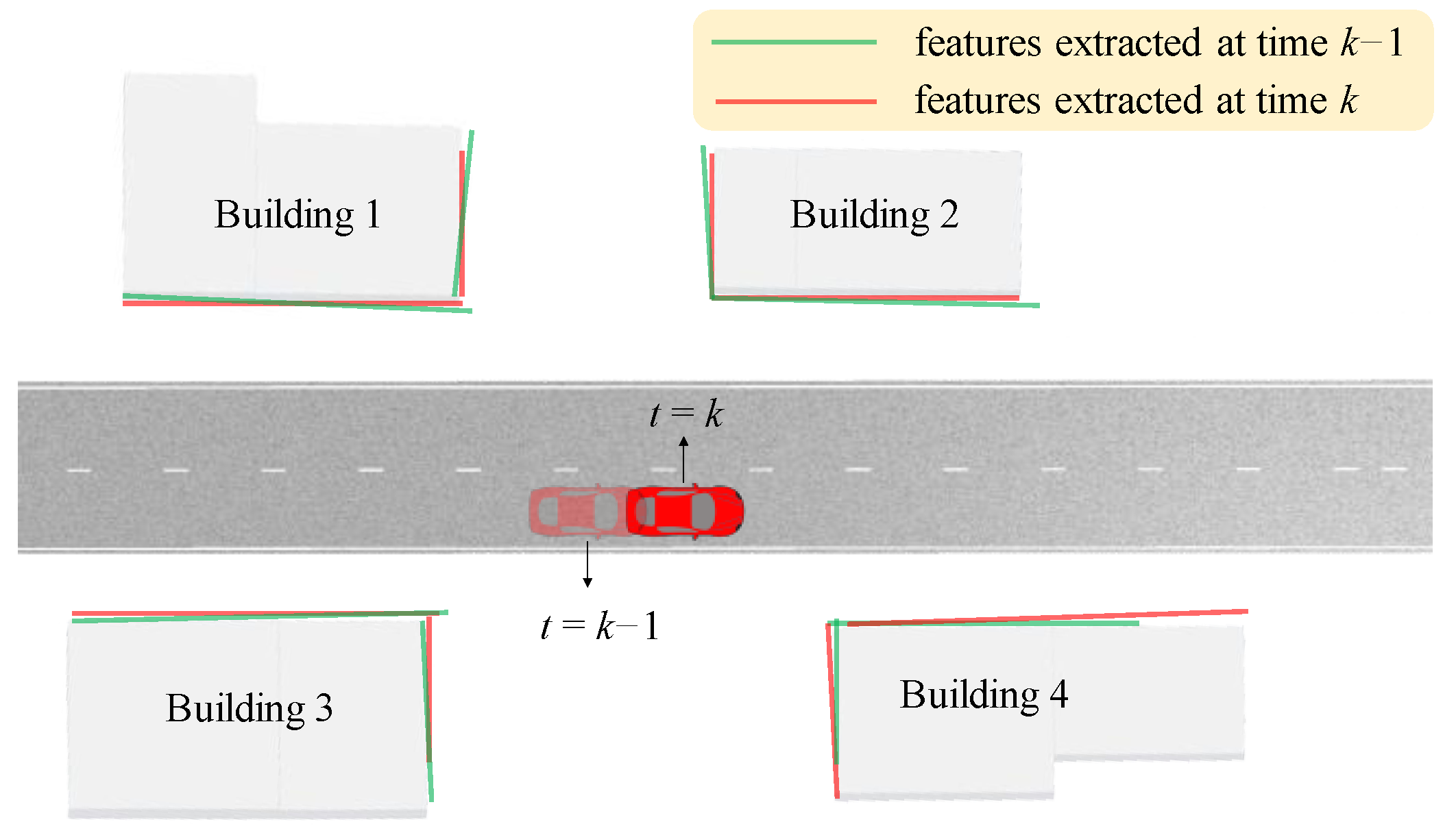
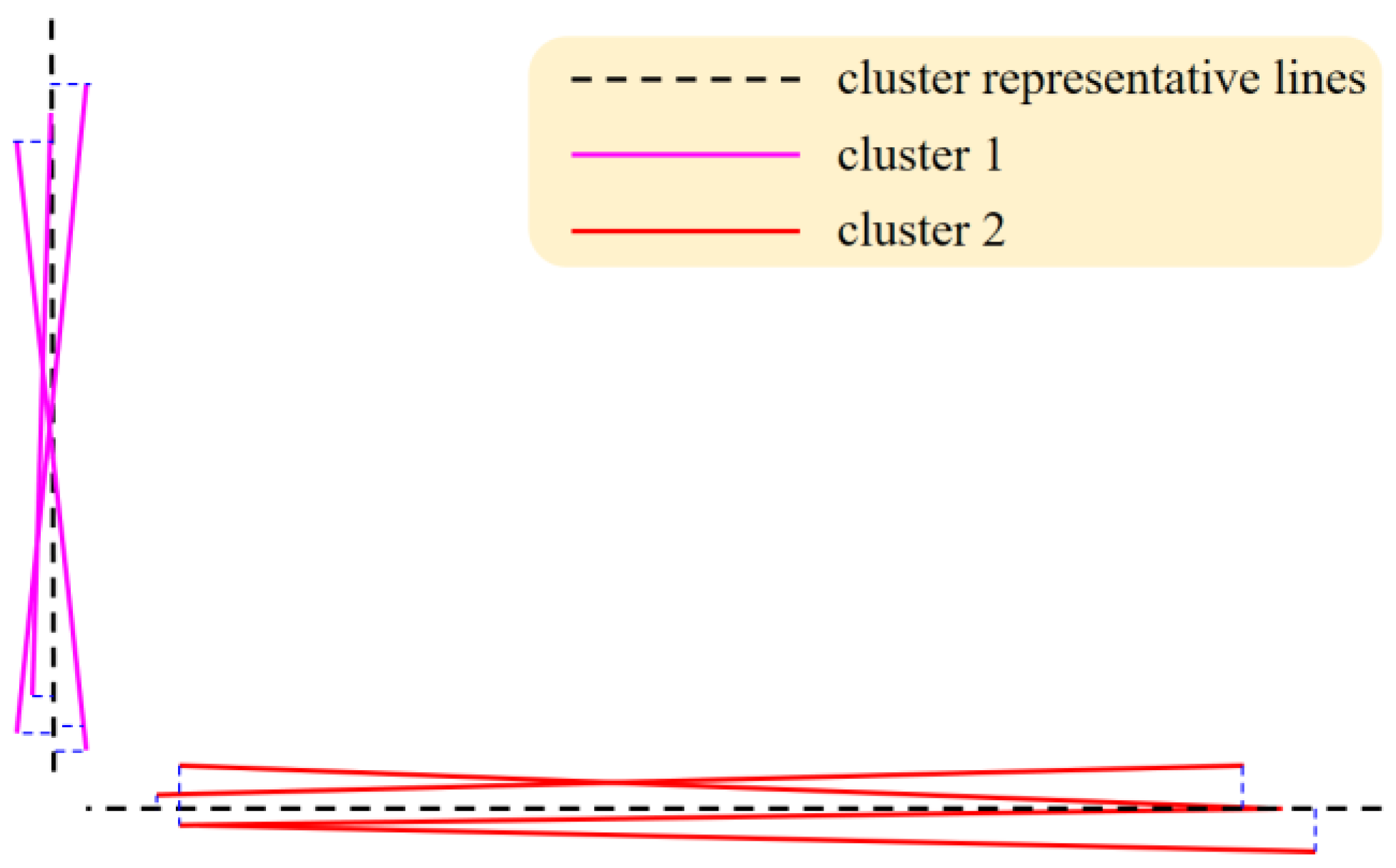
3.1.1. Criterion 1—Small Included Angle
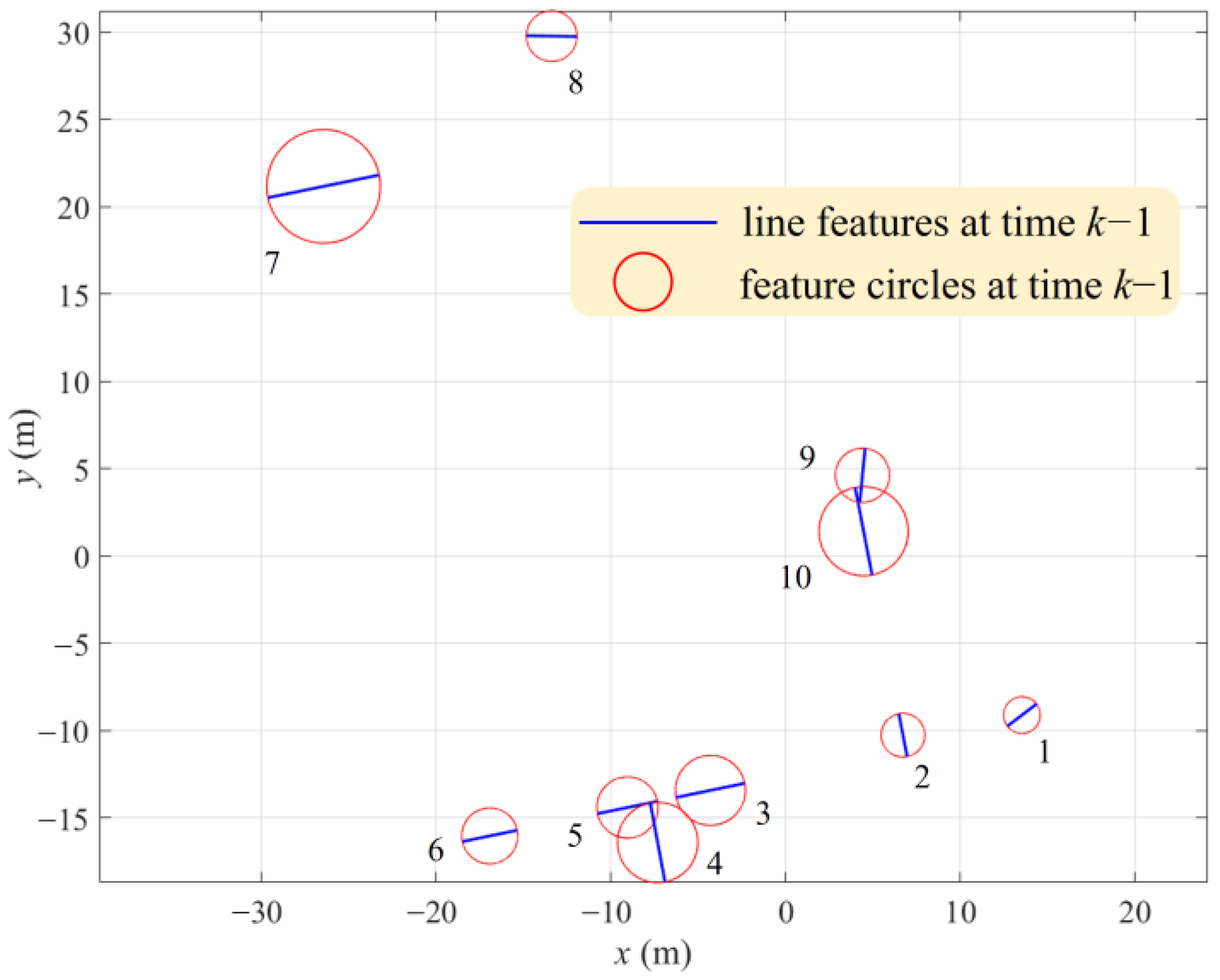
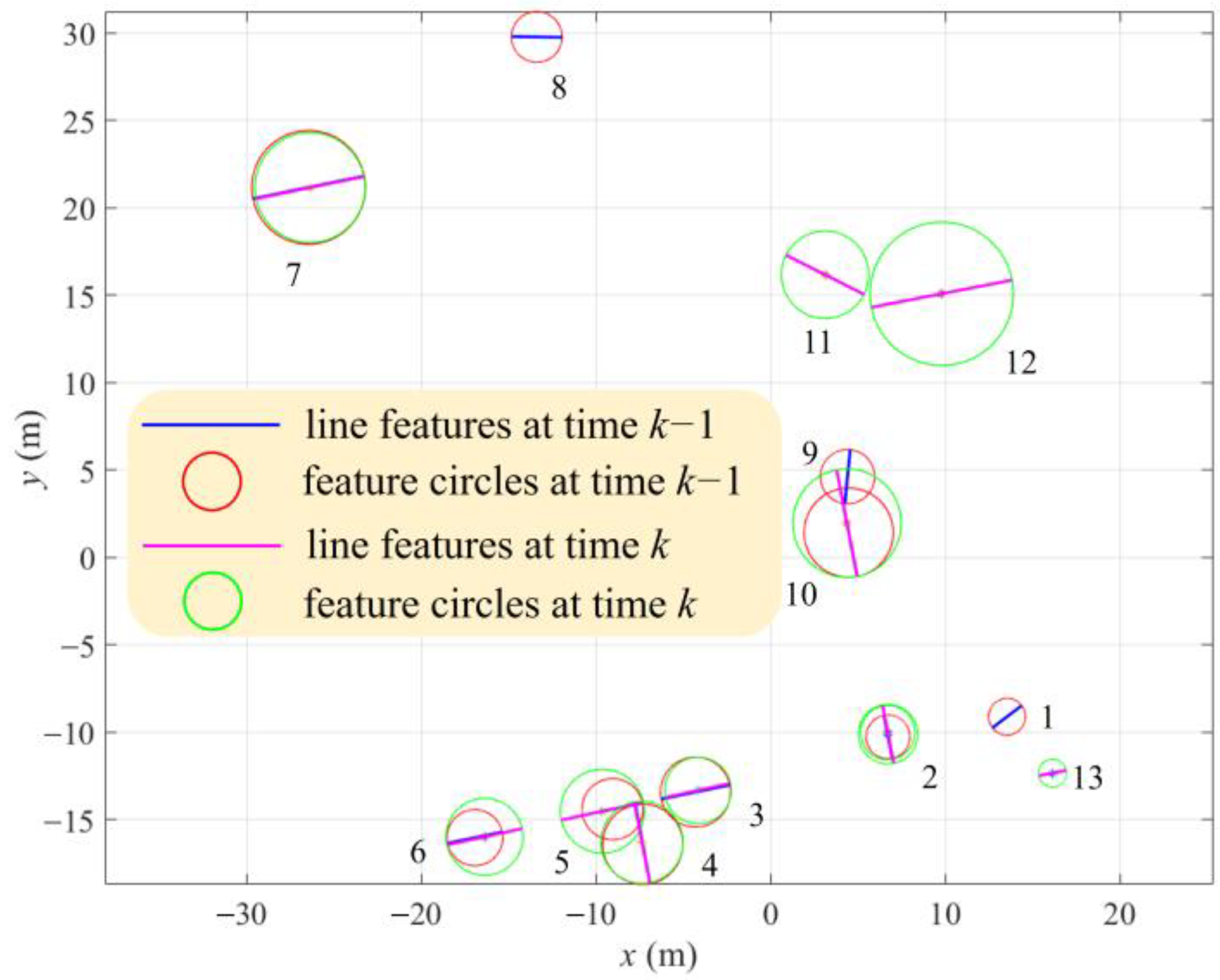
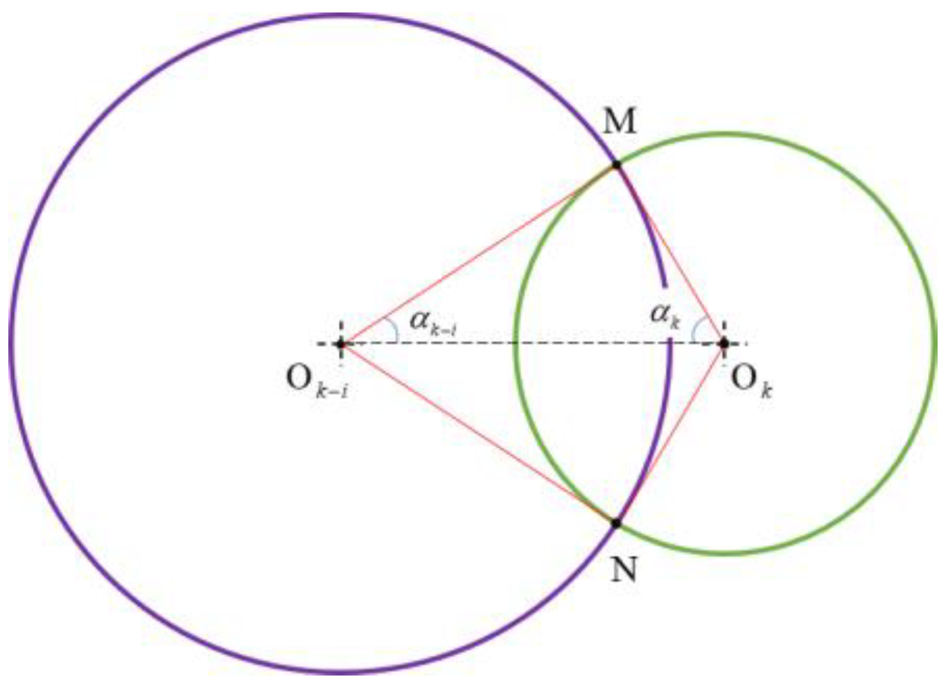
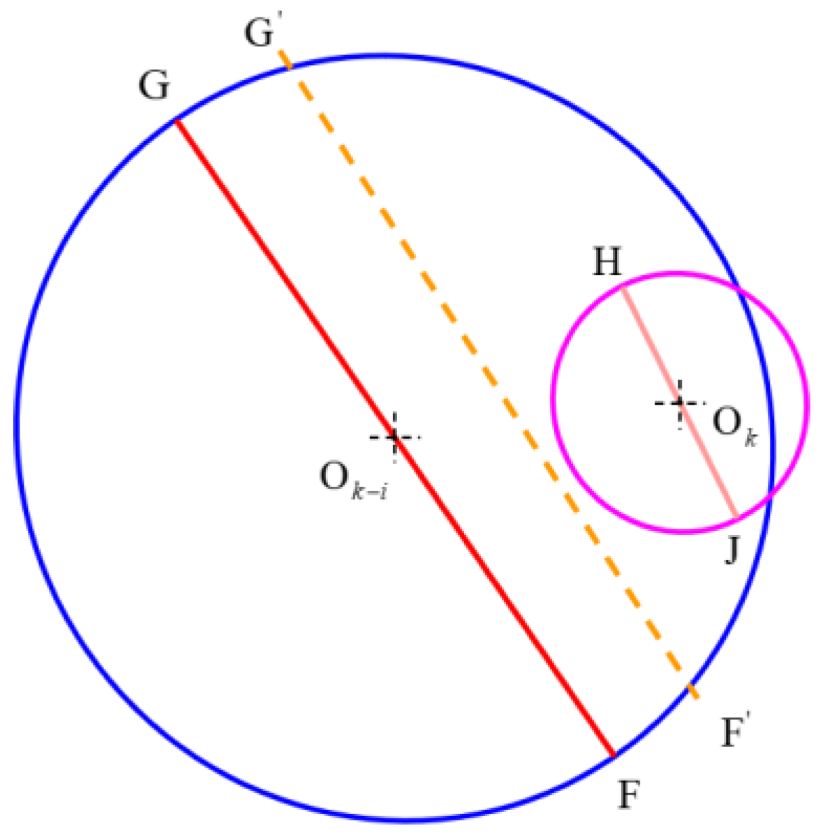
3.1.2. Criterion 2—Large Overlapping Area of Feature Circles
3.1.3. Criterion 3—Small Relative Distance between Features
3.2. Feature Fusion Strategy
4. Results and Discussion
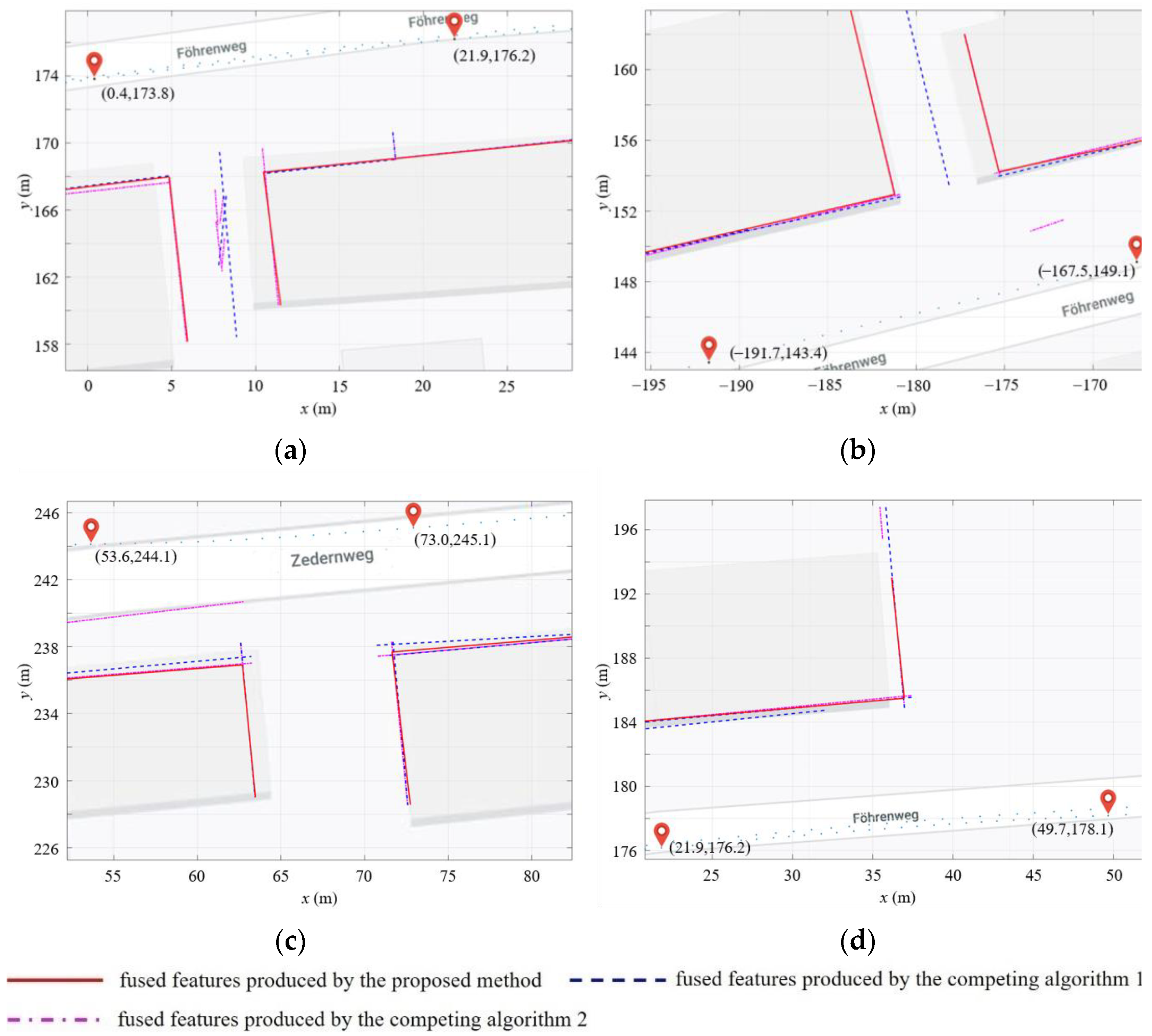
4.1. Comparison in Terms of Conciseness
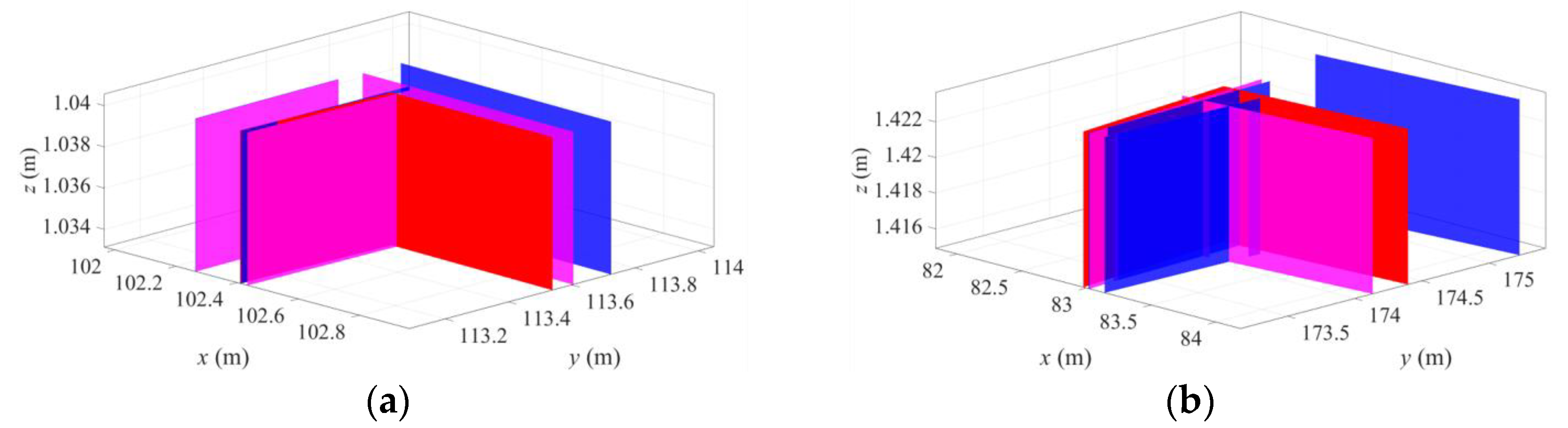
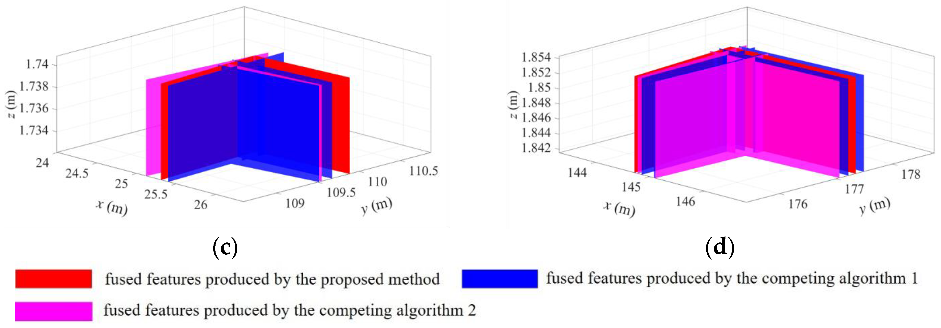
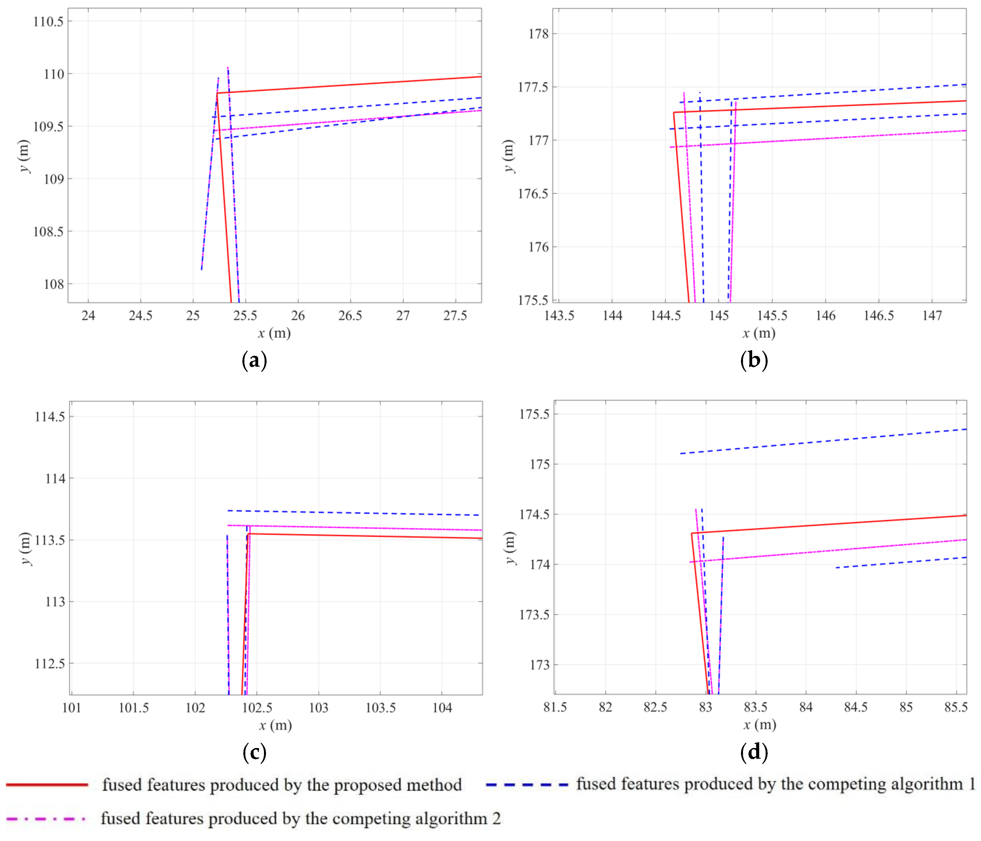
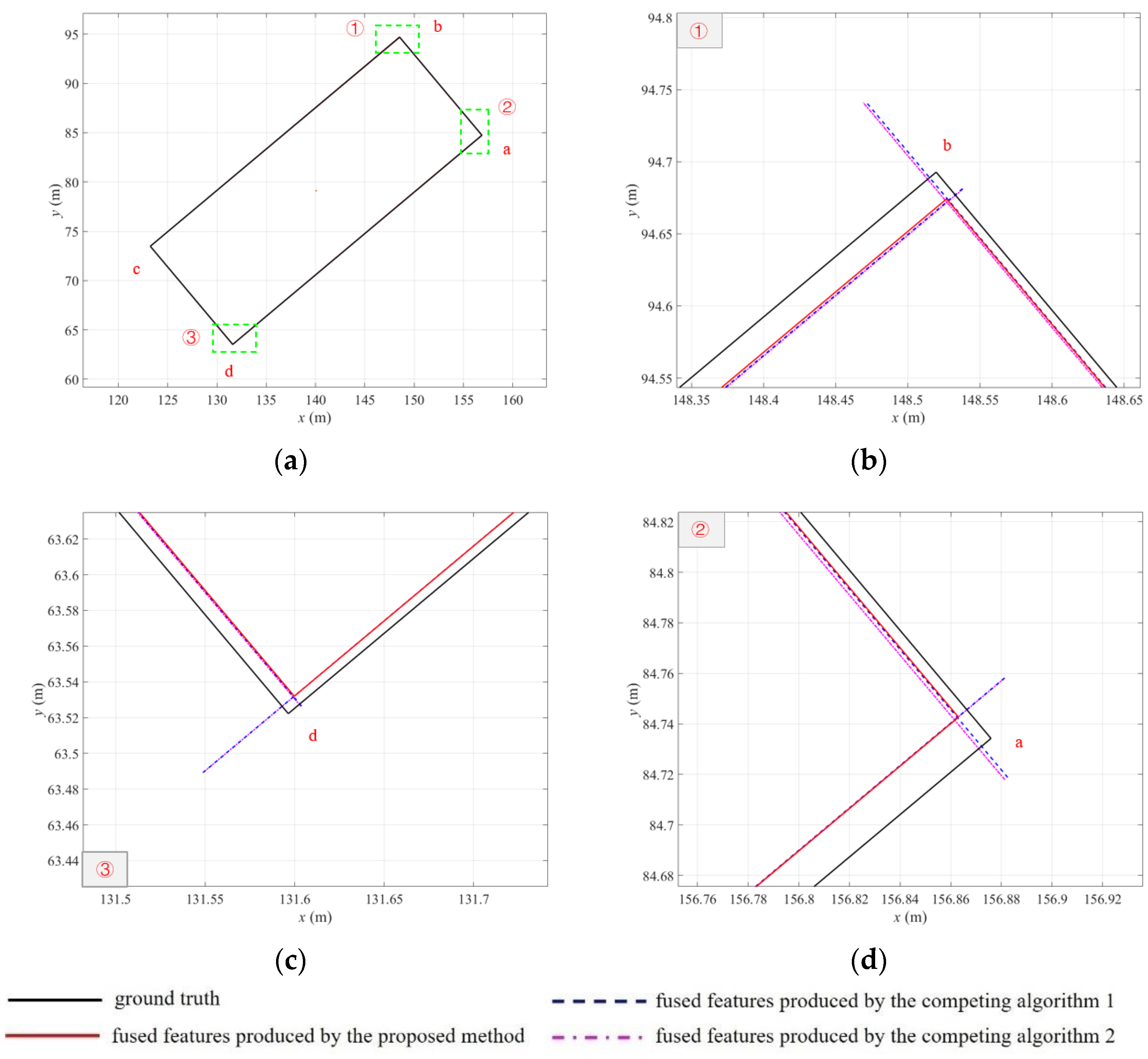
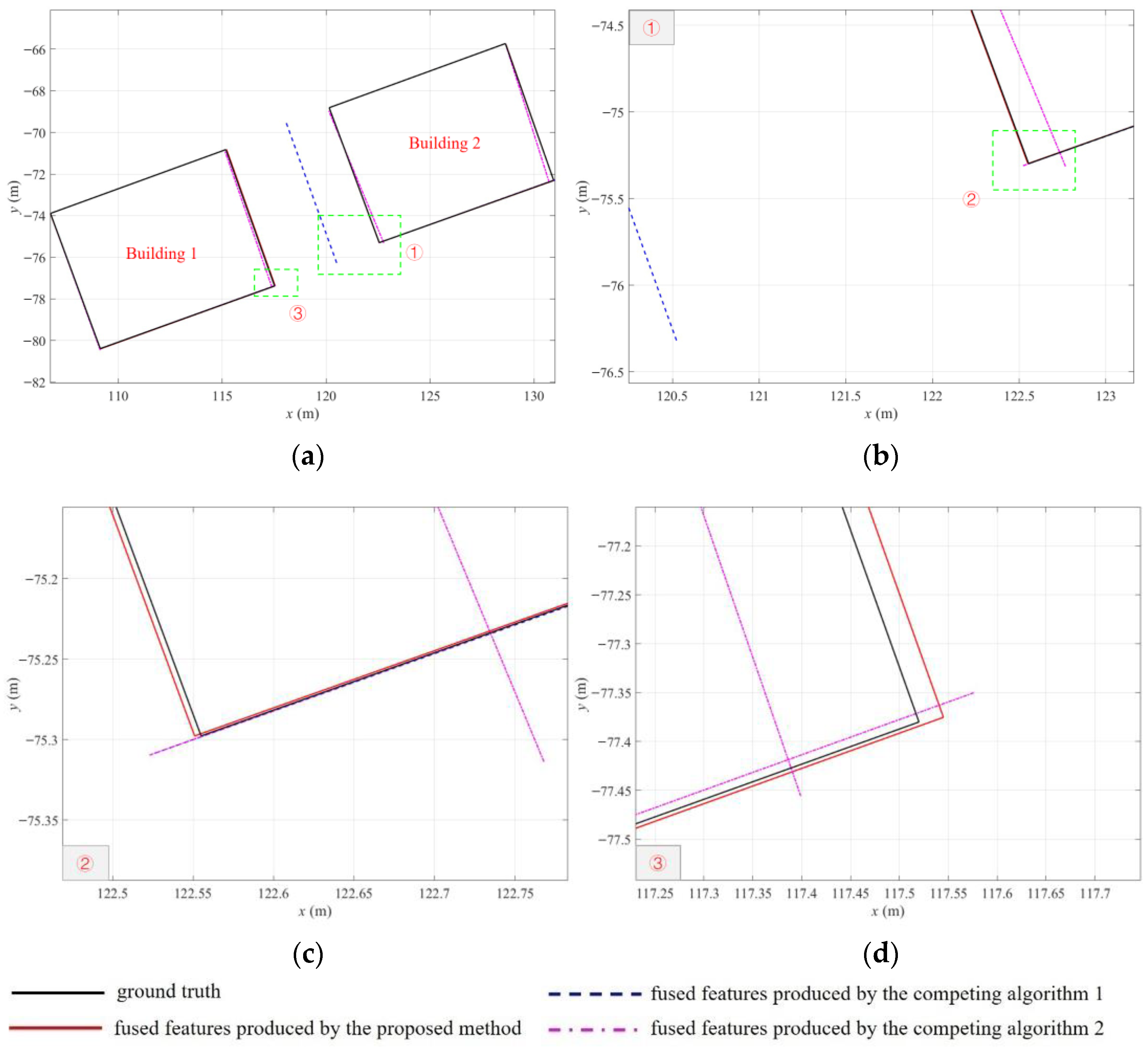
4.2. Comparison in Terms of Accuracy
5. Conclusions and Future Works
Author Contributions
Funding
Data Availability Statement
Conflicts of Interest
References
- Zhao, Y.; Yu, H.; Zhang, K.; Zheng, Y.; Zhang, Y.; Zheng, D.; Han, J. FPP-SLAM: Indoor simultaneous localization and mapping based on fringe projection profilometry. Opt. Express 2023, 31, 5853. [Google Scholar] [CrossRef] [PubMed]
- Gostar, A.K.; Fu, C.; Chuah, W.; Hossain, M.I.; Tennakoon, R.; Bab-Hadiashar, A.; Hoseinnezhad, R. State Transition for Statistical SLAM Using Planar Features in 3D Point Clouds. Sensors 2019, 19, 1614. [Google Scholar] [CrossRef] [PubMed] [Green Version]
- Chen, D.; Weng, J.; Huang, F.; Zhou, J.; Mao, Y.; Liu, X. Heuristic Monte Carlo Algorithm for Unmanned Ground Vehicles Realtime Localization and Mapping. IEEE Trans. Veh. Technol. 2020, 69, 10642–10655. [Google Scholar] [CrossRef]
- Sun, J.; Song, J.; Chen, H.; Huang, X.; Liu, Y. Autonomous State Estimation and Mapping in Unknown Environments with Onboard Stereo Camera for Micro Aerial Vehicles. IEEE Trans. Ind. Inform. 2019, 16, 5746–5756. [Google Scholar] [CrossRef]
- Wen, S.; Zhao, Y.; Liu, X.; Sun, F.; Lu, H.; Wang, Z. Hybrid Semi-Dense 3D Semantic-Topological Mapping From Stereo Visual-Inertial Odometry SLAM with Loop Closure Detection. IEEE Trans. Veh. Technol. 2020, 69, 16057–16066. [Google Scholar] [CrossRef]
- Zubizarreta, J.; Aguinaga, I.; Montiel, J.M.M. Direct Sparse Mapping. IEEE Trans. Robot. 2020, 36, 1363–1370. [Google Scholar] [CrossRef]
- Yu, Z.; Min, H. Visual SLAM Algorithm Based on ORB Features and Line Features. In Proceedings of the 2019 Chinese Automation Congress (CAC), Hangzhou, China, 22–24 November 2019; pp. 3003–3008. [Google Scholar] [CrossRef]
- Campos, C.; Elvira, R.; Rodríguez, J.J.G.; Montiel, J.M.; Tardós, J.D. ORB-SLAM3: An Accurate Open-Source Library for Visual, Visual–Inertial, and Multimap SLAM. IEEE Trans. Robot. 2021, 37, 1874–1890. [Google Scholar] [CrossRef]
- Yuan, C.; Xu, Y.; Zhou, Q. PLDS-SLAM: Point and Line Features SLAM in Dynamic Environment. Remote Sens. 2023, 15, 1893. [Google Scholar] [CrossRef]
- Zi, B.; Wang, H.; Santos, J.; Zheng, H. An Enhanced Visual SLAM Supported by the Integration of Plane Features for the Indoor Environment. In Proceedings of the 2022 IEEE 12th International Conference on Indoor Positioning and Indoor Navigation (IPIN), Beijing, China, 5–8 September 2022; pp. 1–8. [Google Scholar] [CrossRef]
- Li, F.; Fu, C.; Gostar, A.K.; Yu, S.; Hu, M.; Hoseinnezhad, R. Advanced Mapping Using Planar Features Segmented from 3D Point Clouds. In Proceedings of the 2019 International Conference on Control, Automation and Information Sciences (ICCAIS), Chengdu, China, 23–26 October 2019; pp. 1–6. [Google Scholar]
- Yang, H.; Yuan, J.; Gao, Y.; Sun, X.; Zhang, X. UPLP-SLAM: Unified point-line-plane feature fusion for RGB-D visual SLAM. Inf. Fusion 2023, 96, 51–65. [Google Scholar] [CrossRef]
- Yu, S.; Fu, C.; Gostar, A.K.; Hu, M. A Review on Map-Merging Methods for Typical Map Types in Multiple-Ground-Robot SLAM Solutions. Sensors 2020, 20, 6988. [Google Scholar] [CrossRef]
- Sun, Q.; Yuan, J.; Zhang, X.; Duan, F. Plane-Edge-SLAM: Seamless Fusion of Planes and Edges for SLAM in Indoor Envi-ronments. IEEE Trans. Autom. Sci. Eng. 2021, 18, 2061–2075. [Google Scholar] [CrossRef]
- Dai, K.; Sun, B.; Wu, G.; Zhao, S.; Ma, F.; Zhang, Y.; Wu, J. LiDAR-Based Sensor Fusion SLAM and Localization for Autonomous Driving Vehicles in Complex Scenarios. J. Imaging 2023, 9, 52. [Google Scholar] [CrossRef]
- Xie, H.; Zhang, D.; Wang, J.; Zhou, M.; Cao, Z.; Hu, X.; Abusorrah, A. Semi-Direct Multimap SLAM System for Real-Time Sparse 3-D Map Reconstruction. IEEE Trans. Instrum. Meas. 2023, 72, 1–13. [Google Scholar] [CrossRef]
- Xu, Y.; Zhou, L.; Tang, H.; Wu, Q.; Xie, Q.; Chen, H.; Wang, J. Robust and Accurate RGB-D Reconstruction with Line Feature Constraints. IEEE Robot. Autom. Lett. 2021, 6, 6561–6568. [Google Scholar] [CrossRef]
- Sarkar, B.; Pal, P.K.; Sarkar, D. Building maps of indoor environments by merging line segments extracted from registered laser range scans. Robot. Auton. Syst. 2014, 62, 603–615. [Google Scholar] [CrossRef]
- Elseberg, J.; Creed, R.T.; Lakaemper, R. A line segment based system for 2D global mapping. In Proceedings of the IEEE International Conference on Robotics and Automation, Anchorage, Alaska, 3–8 May 2010; pp. 3924–3931. [Google Scholar]
- Amigoni, F.; Li, A.Q. Comparing methods for merging redundant line segments in maps. Robot. Auton. Syst. 2018, 99, 135–147. [Google Scholar] [CrossRef]
- Amigoni, F.; Vailati, M. A method for reducing redundant line segments in maps. In Proceedings of the European Conference on Mobile Robots (ECMR), Mlini/Dubrovnik, Croatia, 23–25 September 2009; pp. 61–66. [Google Scholar]
- Gomez-Ojeda, R.; Moreno, F.; Scaramuzza, D.; Gonzalez-Jimenez, J. PL-SLAM: A stereo SLAM system through the combination of points and line segments. arXiv 2017, arXiv:1705.09479. [Google Scholar] [CrossRef] [Green Version]
- Liu, J.; Meng, Z. Visual SLAM with Drift-Free Rotation Estimation in Manhattan World. IEEE Robot. Autom. Lett. 2020, 5, 6512–6519. [Google Scholar] [CrossRef]
- Gao, H.; Zhang, X.; Li, C.; Chen, X.; Fang, Y.; Chen, X. Directional Endpoint-based Enhanced EKF-SLAM for Indoor Mobile Robots. In Proceedings of the 2019 IEEE/ASME International Conference on Advanced Intelligent Mechatronics (AIM), Hong Kong, China, 8–12 July 2019; pp. 978–983. [Google Scholar]
- Wen, J.; Zhang, X.; Gao, H.; Yuan, J.; Fang, Y. CAE-RLSM: Consistent and Efficient Redundant Line Segment Merging for Online Feature Map Building. IEEE Trans. Instrum. Meas. 2019, 69, 4222–4237. [Google Scholar] [CrossRef] [Green Version]
- Wang, J.; Song, J.; Zhao, L.; Huang, S.; Xiong, R. A submap joining algorithm for 3D reconstruction using an RGB-D camera based on point and plane features. Robot. Auton. Syst. 2019, 118, 93–111. [Google Scholar] [CrossRef]
- Hsiao, M.; Westman, E.; Zhang, G.; Kaess, M. Keyframe-based dense planar SLAM. In Proceedings of the IEEE International Conference on Robotics and Automation (ICRA), Singapore, 29 May–3 June 2017; pp. 5110–5117. [Google Scholar]
- Ćwian, K.; Nowicki, M.R.; Nowak, T.; Skrzypczyński, P. Planar Features for Accurate Laser-Based 3-D SLAM in Urban Environments. In Advances in Intelligent Systems and Computing; Springer: Cham, Switzerland, 2020; pp. 941–953. [Google Scholar] [CrossRef]
- Grant, W.S.; Voorhies, R.C.; Itti, L. Efficient Velodyne SLAM with point and plane features. Auton. Robot. 2018, 43, 1207–1224. [Google Scholar] [CrossRef]
- Pan, L.; Wang, P.F.; Cao, J.W.; Chew, C.M. Dense RGB-D SLAM with Planes Detection and Mapping. In Proceedings of the IECON 2019—45th Annual Conference of the IEEE Industrial Electronics Society, Lisbon, Portugal, 14–17 October 2019; pp. 5192–5197. [Google Scholar]
- Lakaemper, R. Simultaneous multi-line-segment merging for robot mapping using Mean shift clustering. In Proceedings of the 2009 IEEE/RSJ International Conference on Intelligent Robots and Systems (IEEE /RSJ IROS), St. Louis, MO, USA, 10–15 October 2009; pp. 1654–1660. [Google Scholar]
- Geiger, A.; Lenz, P.; Stiller, C.; Urtasun, R. Vision meets robotics: The KITTI dataset. Int. J. Robot. Res. 2013, 32, 1231–1237. [Google Scholar] [CrossRef] [Green Version]


| Map | Number of Fused Features | ||
|---|---|---|---|
| Competing Algorithm 1 | Competing Algorithm 2 | Proposed Algorithm | |
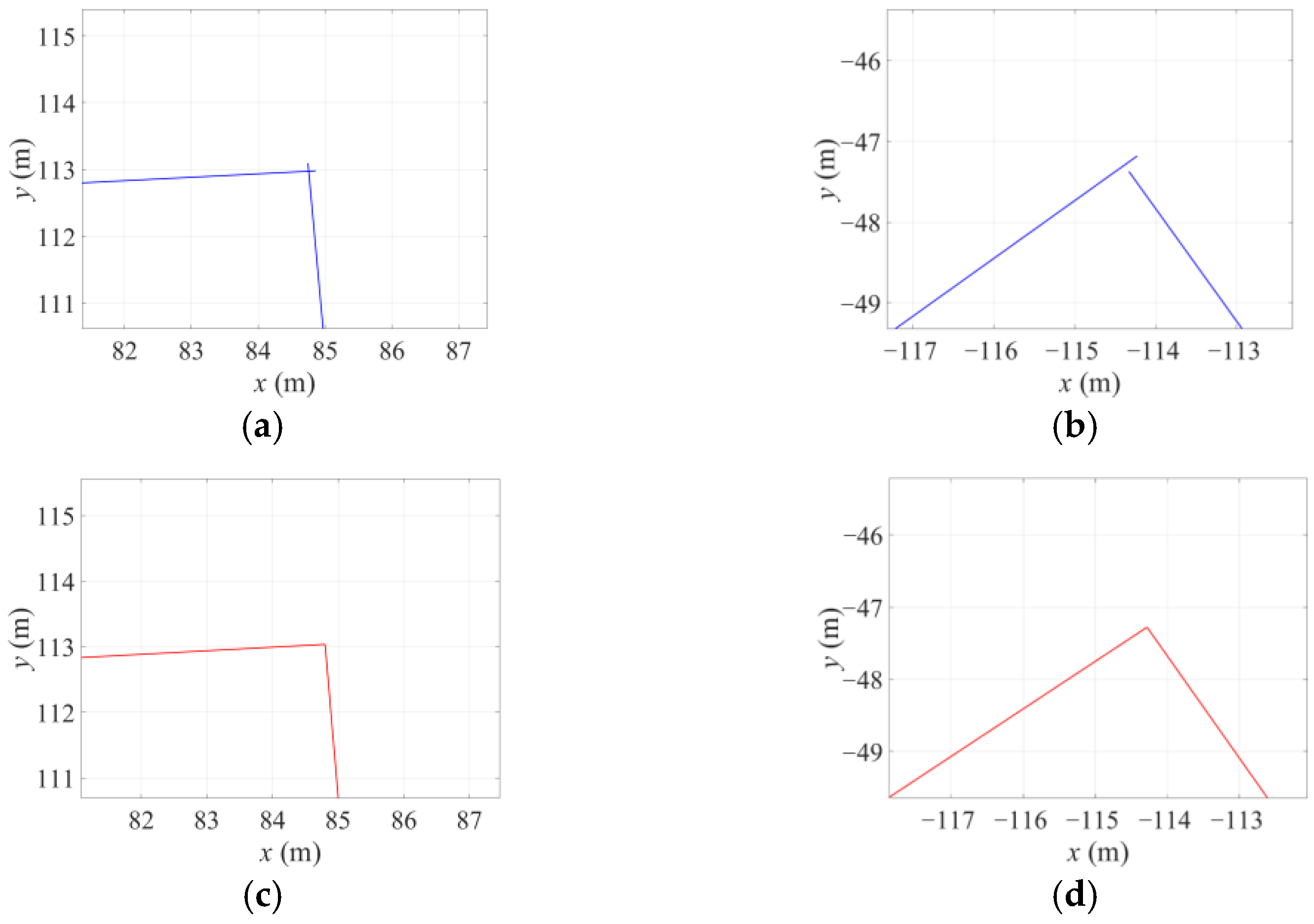
| Figure 11a | 4 | 3 | 2 |
| Figure 11b | 4 | 3 | 2 |
| Figure 11c | 2 | 3 | 2 |
| Figure 11d | 4 | 3 | 2 |
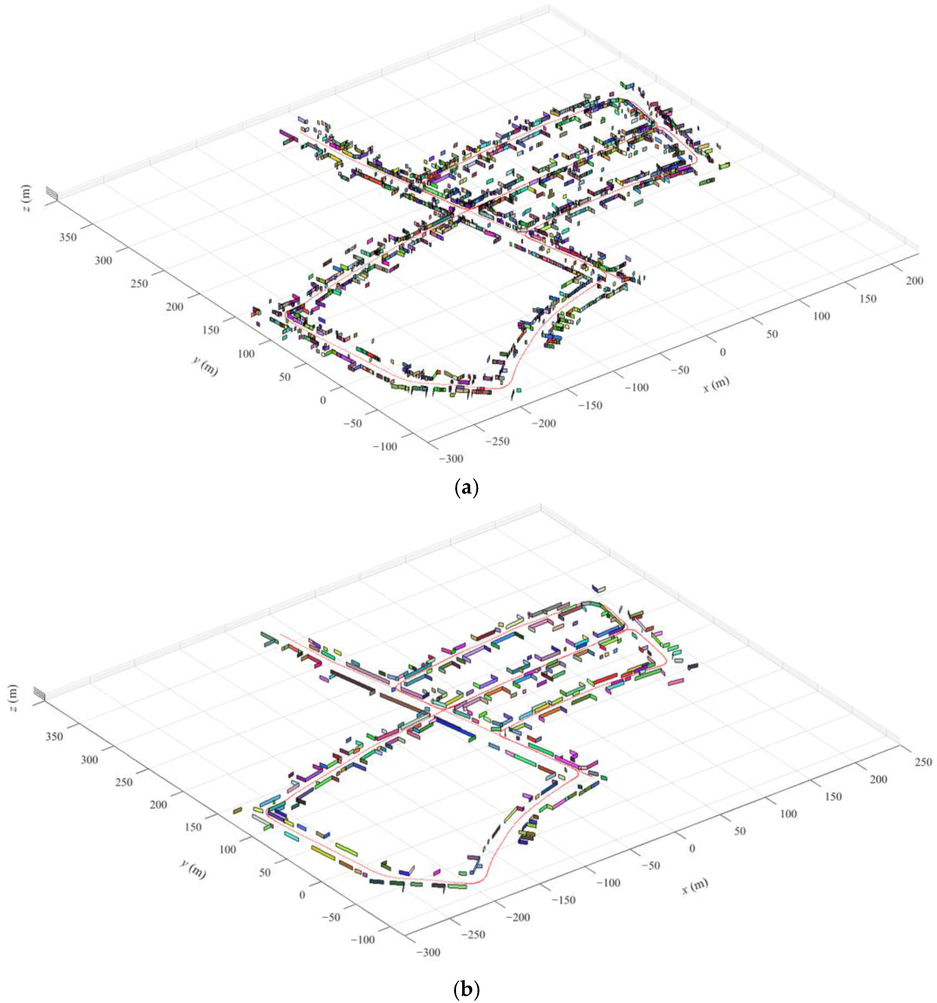
| Global Map | 1333 | 513 | 360 |
| Vertex | Competing Algorithm 1 | Competing Algorithm 2 | Proposed Algorithm |
|---|---|---|---|
| a (m) | 0.0414 | 0.0416 | 0.0310 |
| b (m) | 0.0916 | 0.0917 | 0.0397 |
| c (m) | 0.0196 | 0.0200 | 0.0010 |
| d (m) | 0.0665 | 0.0664 | 0.0212 |
| Competing Algorithm 1 | Competing Algorithm 2 | Proposed Algorithm | |
|---|---|---|---|
| time (s) | 3.24 | 4.68 | 8.45 |
Disclaimer/Publisher’s Note: The statements, opinions and data contained in all publications are solely those of the individual author(s) and contributor(s) and not of MDPI and/or the editor(s). MDPI and/or the editor(s) disclaim responsibility for any injury to people or property resulting from any ideas, methods, instructions or products referred to in the content. |
© 2023 by the authors. Licensee MDPI, Basel, Switzerland. This article is an open access article distributed under the terms and conditions of the Creative Commons Attribution (CC BY) license (https://creativecommons.org/licenses/by/4.0/).
Share and Cite
Li, F.; Fu, C.; Sun, D.; Marzbani, H.; Hu, M. Reducing Redundancy in Maps without Lowering Accuracy: A Geometric Feature Fusion Approach for Simultaneous Localization and Mapping. ISPRS Int. J. Geo-Inf. 2023, 12, 235. https://doi.org/10.3390/ijgi12060235
Li F, Fu C, Sun D, Marzbani H, Hu M. Reducing Redundancy in Maps without Lowering Accuracy: A Geometric Feature Fusion Approach for Simultaneous Localization and Mapping. ISPRS International Journal of Geo-Information. 2023; 12(6):235. https://doi.org/10.3390/ijgi12060235
Chicago/Turabian StyleLi, Feiya, Chunyun Fu, Dongye Sun, Hormoz Marzbani, and Minghui Hu. 2023. "Reducing Redundancy in Maps without Lowering Accuracy: A Geometric Feature Fusion Approach for Simultaneous Localization and Mapping" ISPRS International Journal of Geo-Information 12, no. 6: 235. https://doi.org/10.3390/ijgi12060235