A Spatio-Temporal Dynamic Visualization Method of Time-Varying Wind Fields Based on Particle System

Abstract

The particle system is widely used in vector field feature visualization due to its dynamics and simulation. However, there are some defects of the vector field visualization method based on the Euler fields, such as unclear feature expression and discontinuous temporal expression, so the method cannot effectively express the characteristics of wind field on the temporal scale. We propose a Lagrangian visualization method based on spatio-temporal interpolation to solve these problems, which realizes the fusion and expression of the particle system and the time-varying wind data based on the WebGL shader. Firstly, the linear interpolation algorithm is used to interpolate to obtain continuous and dense wind field data according to the wind field data at adjacent moments. Then, we introduce the Lagrangian analysis method to study the structure of the wind field and optimize the visualization effect of the particle system based on Runge–Kutta algorithms. Finally, we adopt the nonlinear color mapping method with double standard deviation (2SD) to improve the expression effect of wind field features. The experimental results indicate that the wind visualization achieves a comprehensive visual effect and the rendering frame rate is greater than 45. The methods can render the particles smoothly with stable and outstanding uniformity when expressing continuous spatio-temporal dynamic visualization characteristics of the wind field.

1. Introduction

As an essential power source of atmospheric motion, wind participates in almost all atmospheric motions on the Earth’s surface, including air–ground heat exchange and typhoon evolution, etc. The visualization research and analysis of time-varying wind fields plays a vital role in exploring the movement of the atmosphere. Efficient and accurate time-varying wind field visualization has become a challenge due to the complex spatio-temporal evolution of the wind field and the large scale of data storage in the real world. Using the Digital Earth platform to display three-dimensional geographic information is more in line with human cognition of the natural world, so it can help users perceive and understand the dynamic visualization of the global wind field intuitively. Using visualization methods to study and analyze wind field data has important application value and practical significance for observing the temporal and spatial evolution of wind fields.

There are generally two different representations of vector field data, the Euler and the Lagrangian method. The Euler method stores the fluid velocity at locations that are fixed in space and describes the velocity information of the flow at the grid points of certain discretization statically, while the Lagrangian method tracks the individual trajectories of each particle moving with the fluid and describes the trajectories of the flow particles advected by the velocity field [1]. The Euler method usually describes the distribution of the field statically, so it is difficult to describe the dynamic scene of the time-varying wind field vividly. The Lagrangian method integrates large numbers of particles in the time-varying velocity field, and the generated trajectory can dynamically describe the motion of wind particles.

The vector field visualization methods include the following categories: direct visualization, geometric visualization, texture-based visualization, and particle system-based visualization [2]. The direct visualization method adopts repeatable icons to represent information in the vector field, usually using arrows and icons with sharp corners to represent the direction and magnitude of the field at different positions [3,4]. The geometric visualization method uses different geometric elements, such as streamlines, surfaces, and tubes, to simulate field characteristics [5]. The texture visualization method performs convolution operation on the vector field information and filter on the random noise texture [6], which represents the vector field with a continuous and consistent dense texture. The particle system method simulates irregular objects using large numbers of randomly distributed and constantly moving particles with specific properties [7,8]. Time-varying data visualization has been a challenging area due to the size of the datasets. Scholars have carried out some related research work on time-varying visualization. Chen [9] proposed a framework of the two-dimensional time-varying vector field, and realized a better modeling effect of the time-varying vector field by introducing the spatio-temporal algorithm to calculate the keyframes. Joshi [10] designed a simple visualization method for time-varying datasets based on illustration-inspired techniques. Hou [11] visualized the three-dimensional time-varying flow field by combining the three-dimensional line integral convolution algorithm with the direct volume rendering technology. The efficiency of experiments on the visualization of time-varying data field is remarkably improved by the improvement of large dataset compression techniques. The above results make contributions in the expression of time-varying data, but they only verify the visualization effect of time-varying data, and cannot be combined with three-dimensional geographic spatial data. Thus, it is difficult to express the spatio-temporal attributes of the global wind field and there is poor interaction with geographic space in the existing results.

In addition, studies have developed many visualization prototype systems and there have been numerous achievements in the field of visualization in scientific computing. Hu et al. [12] constructed a multi-dimensional dynamic visualization system of typhoons based on the virtual Earth platform to realize the dynamic expression of typhoon data. Liu et al. [13] visualized meteorological data based on the virtual Earth analysis system, including flow direction quantity, particle tracking, cross section analysis, streamline, path animation, volume rendering, and other methods. Mei et al. [14] designed a visualization system for atmospheric data, AVIS, which supports the visualization of a variety of data fields and uses streamline methods to visualize wind vector field data. Francesco et al. [15] introduced the NASA Web World Wind System, which uses directional arrows to represent the direction of the wind and color grading to represent the size of the wind to map the global wind field. Liu [16] realized the dynamic visualization of the ocean vector field on a 3D virtual Earth platform based on the particle system and SPH (smoothed particle hydrodynamics) method, and improved the rendering speed of a large-scale 3D vector field by using WebWorker multithreading and the GPU acceleration algorithm of the multi-frame buffer. Tan et al. [17] adopted the video compression coding method to realize the efficient transmission of multi-layer time series data, and realized the dynamic interactive visualization of the atmospheric wind field based on the particle tracking moving streamline method. Wang et al. [18] proposed an automated data processing pipeline and achieved effective visualization of vector-based earth science data, which integrates novel strategies including random seeding, finer-granularity parallelization, and real-time rendering. Yao et al. [19] proposed a frame buffer visualization method with improved strategies based on WebGL. Chen [9] presented a novel visualization framework that combines the advantages of clustering methods and illustrative rendering techniques to generate a concise depiction of complex flow structures. Chandler [20] presented a method for tracing pathlines in particle-based flow fields, using the particle trajectories to compute pathlines seeded at arbitrary locations. Fang et al. [4] proposed a multi-scale mapping method based on real-time feature streamlines, which improved the stability and uniformity of the seed point layout. Li [21] introduced a web-based platform for visualizing multidimensional time-varying climate data on a virtual globe. Wind field vector data visualization has become a research hotspot. At present, the earth system (url: earth.nullschool.net, accessed on 1 January 2023) and windy system (url: windy.com, accessed on 1 January 2023) are popular wind field data visualization platforms with good visualization effects and rich functions. However, the performance limitations of the platforms, such as the small number of particles and the lack of acceleration mechanism, are very unfavorable to the application and analysis of wind field data. We improve the wind visualization method based on the particle system in the web environment and associate it with graphics hardware to achieve better visualization quality.

Visualization based on the Euler method has a good representation effect for the static vector field, but the time-varying dynamic characteristics of the wind field Euler-based method is incoherent and discontinuous. Moreover, the traditional texture method visualization scheme based on line integral convolution is particularly computationally intensive and inefficient due to the large scale and long duration of wind field data. This paper introduces the Lagrangian method with continuous time dimension to solve those defects. The particle streamline tracing in time-varying fields is implemented through numerical integration of the vector wind field.

In this paper, we propose a dynamic visualization framework of time-varying wind fields using the Lagrangian method based on the particle system, and take the global wind field data as the research object. The time-varying wind field is integrated into the three-dimensional virtual Earth scene for visual expression. The Lagrangian time-varying wind field is constructed based on continuous time-varying vector wind field data, and the GPU-based parallel particle tracking acceleration method is implemented to realize the large-scale, high-efficiency, and refined time-varying wind field visualization method in the virtual Earth. In addition, the Runge–Kutta method is used to optimize the particle trajectory, and the nonlinear color mapping method based on double standard deviation is used to optimize the wind field visualization expression, so the visualization effect is better and smoother. This paper’s primary characteristics are as follows: realizing the dynamic visualization of continuous time-varying wind fields based on the spatio-temporal linear interpolation algorithm, and designing and implementing a nonlinear color mapping method to optimize the rendering effect of wind field particles. In addition, GPU-accelerated particle parallel operation based on the task parallel strategy is realized, which improves the computational efficiency of the particles. The rest of the paper is organized as follows: the materials and methods are introduced in Section 2, including technical route, experiment framework details, and methods introduction. The experiments and results are given in Section 3. Finally, the conclusions of the experiments are discussed in Section 4.

2. Materials and Methods

2.1. Wind Field Data

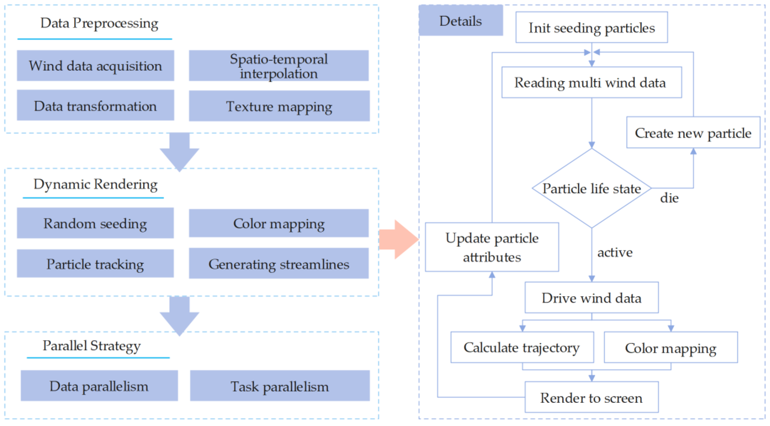
Generally, large-scale monsoon circulation and mesoscale typhoons are unique phenomena of the wind field, ranging from days to months. The land and ocean absorb heat and dissipate heat at different speeds due to the distribution of surface land and ocean in a large area, and the prevailing wind direction or air pressure system will have obvious differences when this situation extends across a long period of time due to the difference in seasonal weather, and the seasonal variation of wind direction or air pressure system is monsoon circulation. A typhoon is a kind of tropical cyclone, which is a low-pressure vortex that occurs on tropical or subtropical oceans. It often causes high winds, heavy rains, and storm surges. In addition, typhoons are significant for improving freshwater supply configuration.

The time-varying wind data (

Table 1. Summary of the wind data.

Option	Parameter
Spatial resolution	0.25° × 0.25°
Temporal resolution	1 h
Longitudinal range	180° W–180° E
Latitudinal range	90° S–90° N
Dimension	1440 × 720 pixels

) in this paper are derived from the global wind field forecast data, provided by the South China Sea Information Center of State Oceanic Administration. The temporal resolution is 1 h and the spatial resolution is 0.25° × 0.25°. The original data format is NetCDF, which is a common binary coded file format for exchanging and storing regularly distributed data. It is widely used in meteorological numerical forecasting products. The wind field data consist of a zonal wind U component and meridional wind V component. According to the requirements of the visualization experiments, the wind field data are from 12 April, 2 July, 14 October 2022 and 10 January 2023. Since the original wind field data are in a binary compression format and the amount of data is large, they are not suitable for network data transmission. Thus, it is necessary to convert the original data format while maintaining the accuracy. The original wind data are converted into texture data. The texture size of the wind field data is 1440 × 720 pixels, which is the same as the original data arrangement. The data size of the original wind field at a single moment is about 4 MB, while the texture data are only about 40 KB. The compressed texture data are convenient for data analysis and transmission.

2.2. Framework

The overview diagram of the spatio-temporal dynamic visualization of the time-varying wind field is shown in Figure 1. This method can efficiently complete the dynamic rendering of wind data with parallel strategy and GPU acceleration. The method mainly consists of three subsections: data preprocessing, dynamic rendering, and parallel strategy. The detail dynamic rendering process is shown on the right side of Figure 1. The arrows represent the workflow direction in the drawing program.

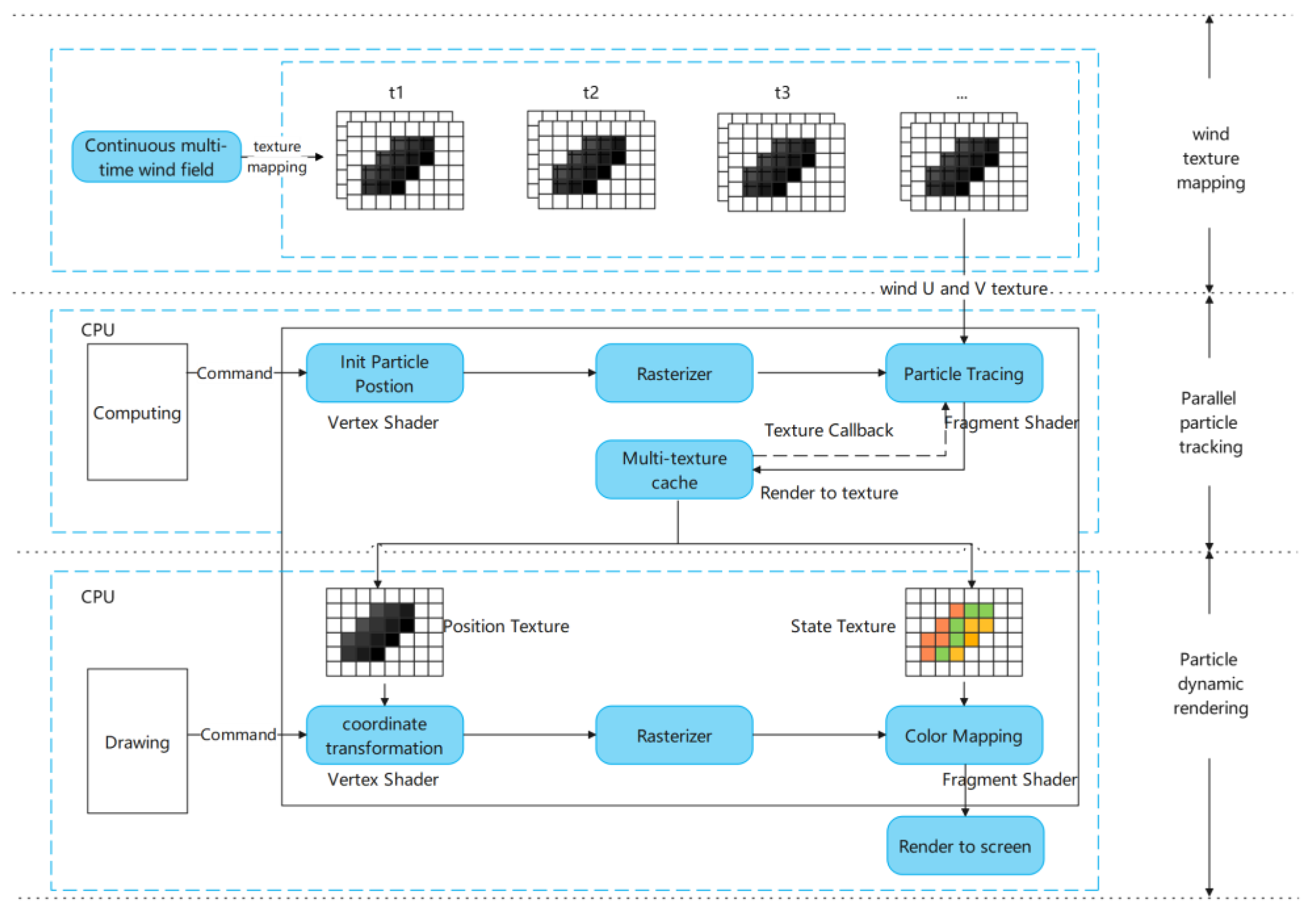
• Data preprocessing: The core of data preprocessing is to analyze the sequential wind field data. We need to perform data interpolation, refine the data resolution, and convert a series of wind field data into multi-layer texture data as input data to drive the movement of wind field particles.
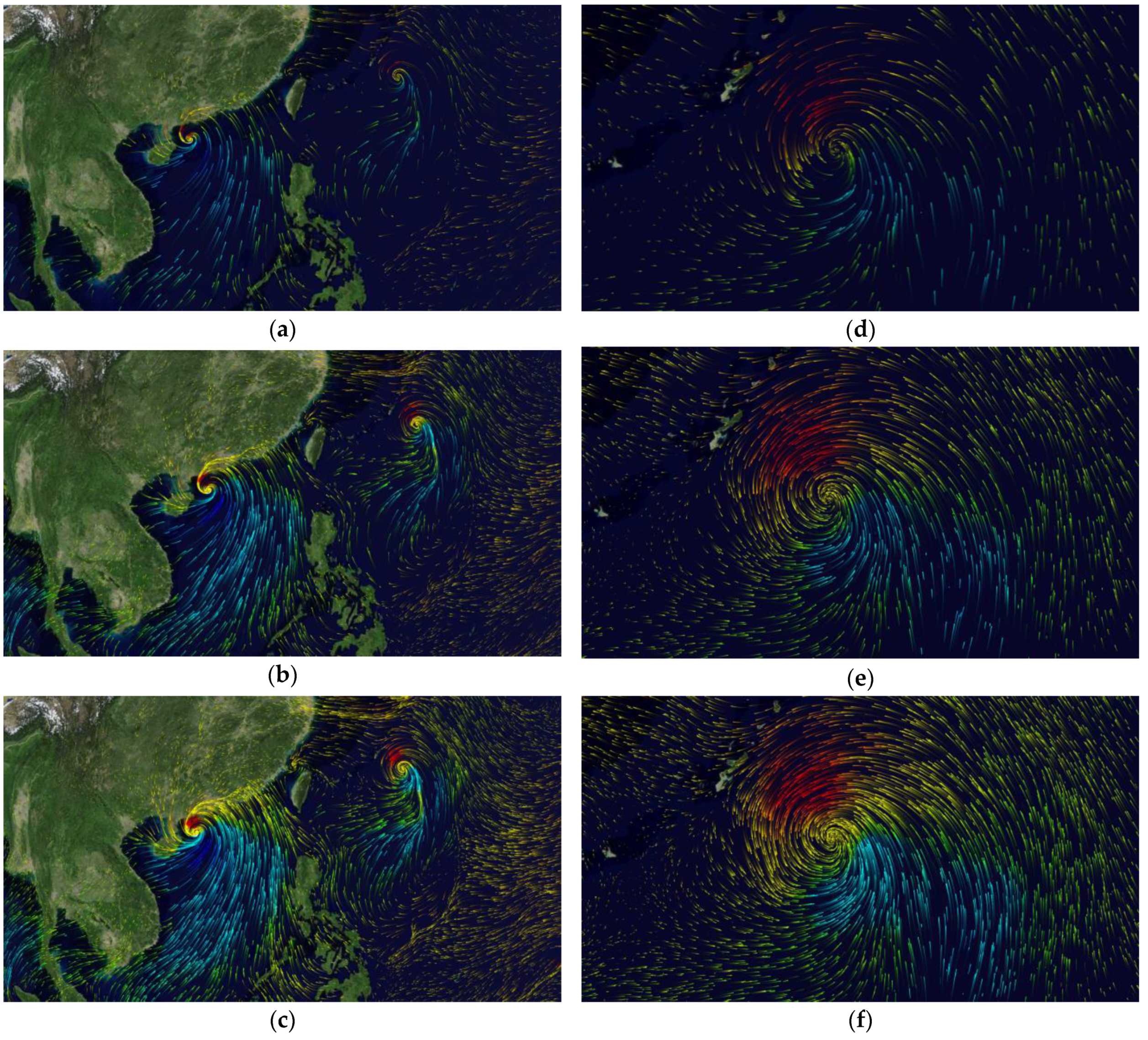
• Dynamic rendering: The particle trajectory is smoothed by the fourth-order Runge–Kutta method, and the time-varying characteristics of the wind field are retained. Users can obtain a good dynamic visual perception. According to the particle seed point distribution, particle trajectory step size, and particle symbol system, the time-varying wind field visualization scheme is customized. The visualization effect of wind particles is further improved based on the nonlinear color mapping method.
• Parallel strategy acceleration: The computing power and rendering tasks are allocated to several processes based on the data parallel strategy and task parallel strategy. The core of parallelism is to allocate the whole processing task, and these subtasks can be executed independently and in parallel on a large scale to accelerate computation.

2.3. Methodology

In this section, the spatio-temporal linear interpolation algorithm is discussed in detail. The particle system efficient rendering based on the data parallelism strategy and task parallelism strategy is introduced, and the particle trajectory is optimized with the fourth-order Runge–Kutta method. Then, the improved visualization strategy is proposed based on nonlinear color mapping.

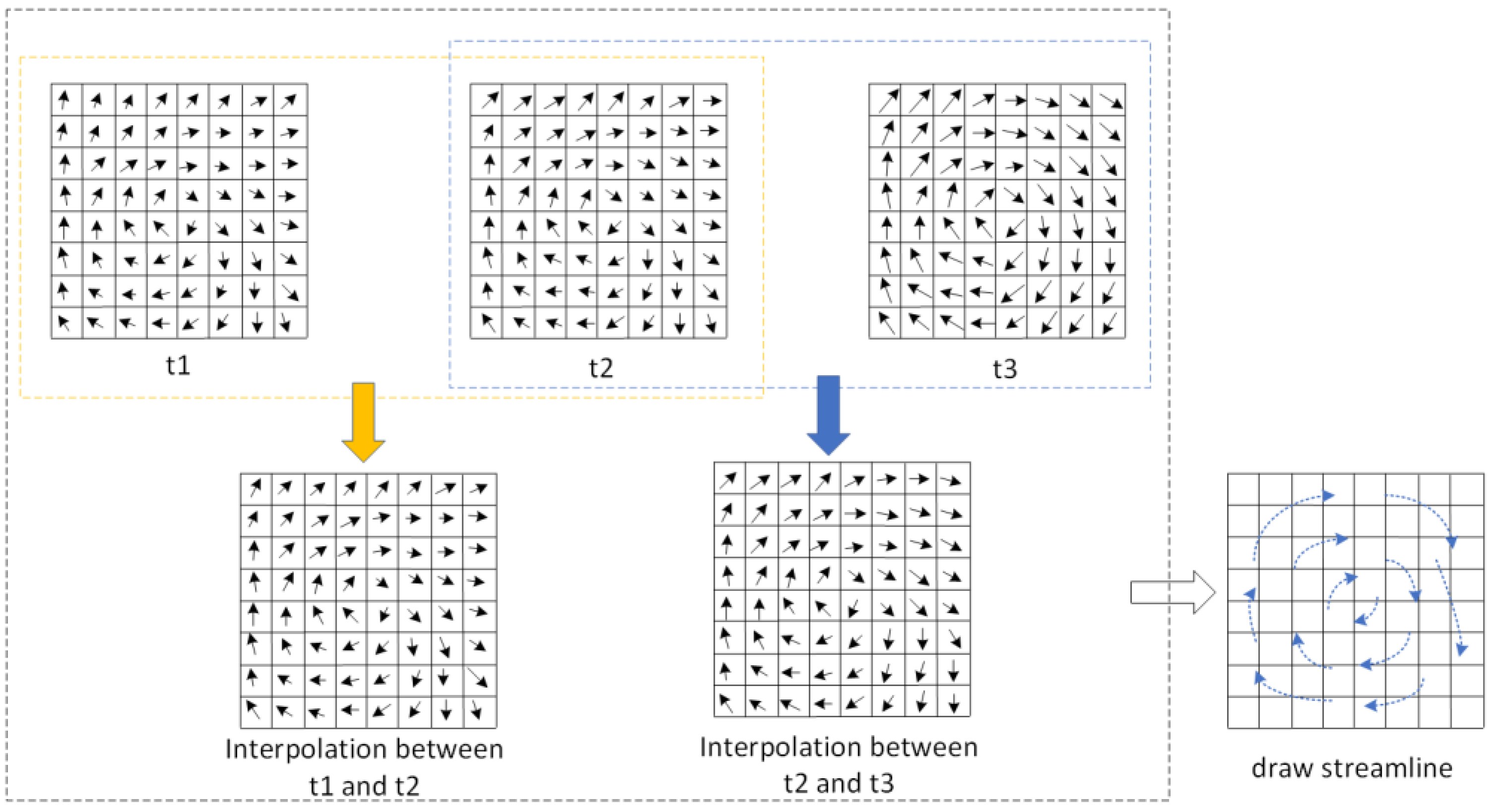
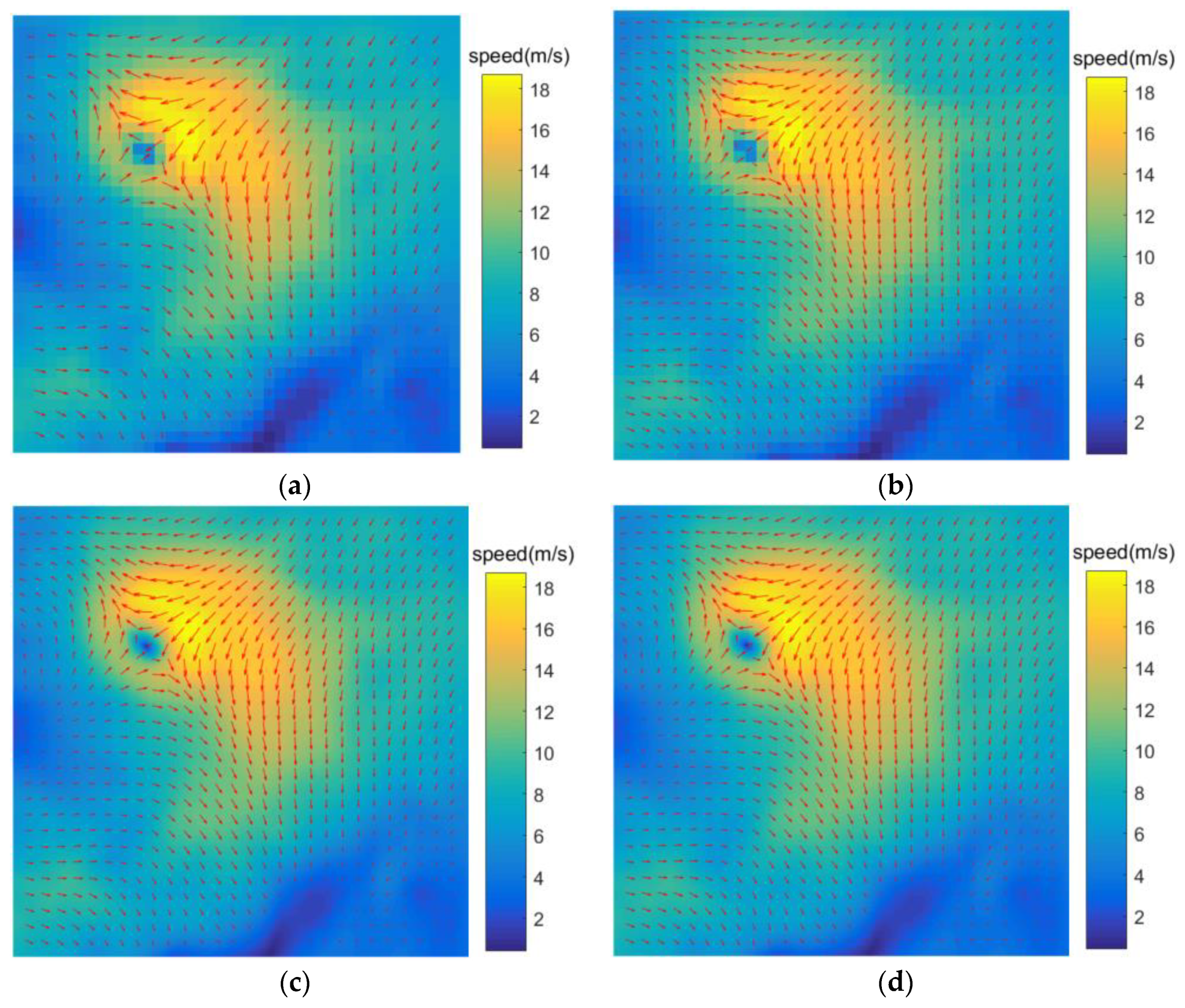
2.3.1. Spatio-Temporal Interpolation Method for Wind Field

Due to the limitation of the resolution of the raw wind field, the number of wind UV textures is fixed, while the streamlines are drawn continuously. The interpolation method is used on the original data to make the wind field smooth and obtain a better visualization effect for the long time series wind field visualization. The spatio-temporal resolution is further improved by interpolating the wind field in spatial and temporal dimensions to fulfil the requirement of time-varying wind field visualization. A bilinear interpolation algorithm is used to enhance the spatial resolution, and a time series interpolation algorithm is used to fill in the wind field data at any intermediate moments.

The interpolation method for the wind field is linearly interpolated (Equation (1)) in the temporal dimension and bilinearly interpolated (Equation (2)) in the spatial dimension. As shown in Figure 2, we interpolate the data on the time axis to achieve a smooth transition between the two key frames and draw a continuous wind field particle trajectory. The black arrow indicates the direction, and the length of the arrow indicates the velocity in Figure 2. The faster the velocity, the longer the arrow. We interpolated between two keyframes data to get a new intermediate keyframe, combining a series of consecutive data to draw the blue streamlines in the same area.

$${\mathrm{S}}_t=S_{t0}\times (1-\frac{t-t_0}{t_1-t_0})+S_{t1}\times (\frac{t-t_0}{t_1-t_0})$$

(1)

$$S_{(x,y)}=S_{(x1,y1)}\times \frac{(x_0-x)(y_0-y)}{(x_0-x_1)(y_0-y_1)}+S_{(x0,y1)}\times \frac{(x-x_1)(y_0-y)}{(x_0-x_1)(y_0-y_1)}+S_{(x1,y0)}\times \frac{(x_0-x)(y-y_1)}{(x_0-x_1)(y_0-y_1)}+S_{(x0,y0)}\times \frac{(x-x_1)(y-y_1)}{(x_0-x_1)(y_0-y_1)}$$

(2)

In Equation (1), $S_{t0}, S_{t1}, S_t$ are the speed at the previous moment, the next moment, and the middle moment. $t_0, t_1,t$ are the time at the previous moment, the next moment, and the middle moment.

In Equation (2), $S_{\left(x,y\right)}$ is the speed value at the point $\left(x,y\right)$. $x,y$ are the coordinate position in the Cartesian coordinate system.

According to the critical point theory proposed by Helman and Hesselink [22], the critical point, also known as singularity, is an important feature in vector field. The critical point refers to the position where each component in the vector field is zero, which is generally divided into the saddle, repelling node, attracting node, attracting focus, repelling focus, and center according to the topology.

Stephen Mann [23] used a geometric algebra method to calculate the Poincaré index of the mesh element. This algorithm can accurately detect the critical point, but is difficult to understand and time-consuming to compute. The calculation process is simplified by calculating the wind direction angle difference. The sum of angle difference refers to the calculation of the grid after traversing the wind direction difference between adjacent points to sum the results. In Equation (3), $ind$ is the sum result index of angle difference, $\mathsf{\Delta }\tau$ is the angle difference based on arc degree, and $n$ is the count of angle difference between adjacent angles. The wind direction angle difference is positive or negative; the angle difference is positive when the wind direction is clockwise change and the angle difference is negative when the wind direction is counterclockwise change. According to the sum index of angle difference, the regional grid is divided into two categories, $ind$ = 0 and $ind$ ≠ 0. It can be considered that the wind field in the region is in the same direction when the index $ind$ is 0. There may be a closed annular wind field in the region when $ind$ is not 0. In the Figure 3, a, b, c, and d represent the different flow directions located in adjacent positions; in general, the bigger the velocity, the longer the arrow. $\mathsf{\Delta }\tau \left(b-a\right)$ is the difference between the angles of the two directions a and b, and the value is in radian unit.

$$ind={\displaystyle \sum _{i=1}^n\frac{\Delta {\tau }_i}{2\pi }}$$

(3)

The interpolation algorithm of vector field is different from that of scalar field. Vector field is the synthetic result of velocity and direction. We adopt two interpolation algorithms according to the distribution characteristics of the wind field grid. When $ind$ is 0, considering the continuity of vector field change, we use the vector expression method based on the polar coordinate system to interpolate the wind speed and wind direction, respectively, which ensures that the change in wind field is continuous. When $ind$ ≠ 0, there may be a critical point inside the grid cell, so we decompose the wind vector into U and V components on the Cartesian coordinate system, and perform linear interpolation on the U and V component, respectively, to ensure that the critical characteristics inside the grid cell will not be lost. U is a component in the east–west direction and V is a component in the north–south direction.

The rendering effect of the direct representation method is often poor due to the limitation of the original wind field dataset resolution. In this study, the linear interpolation algorithm is used to optimize the data density of the wind field. In addition, the interpolation algorithm quickly obtains the interpolation result of the position to be predicted through the index. The correlation between the data predicted by the interpolation results is strong.

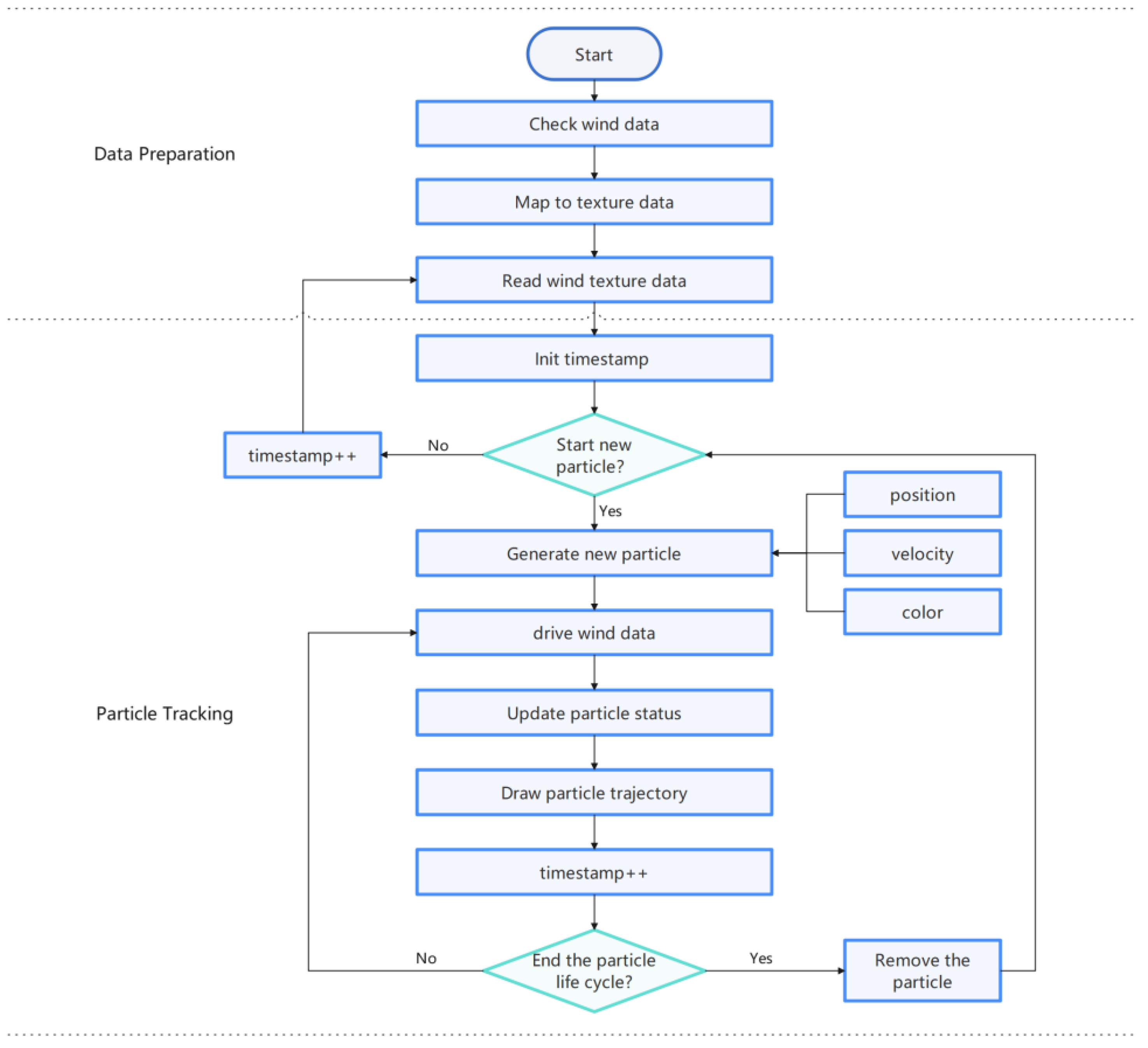
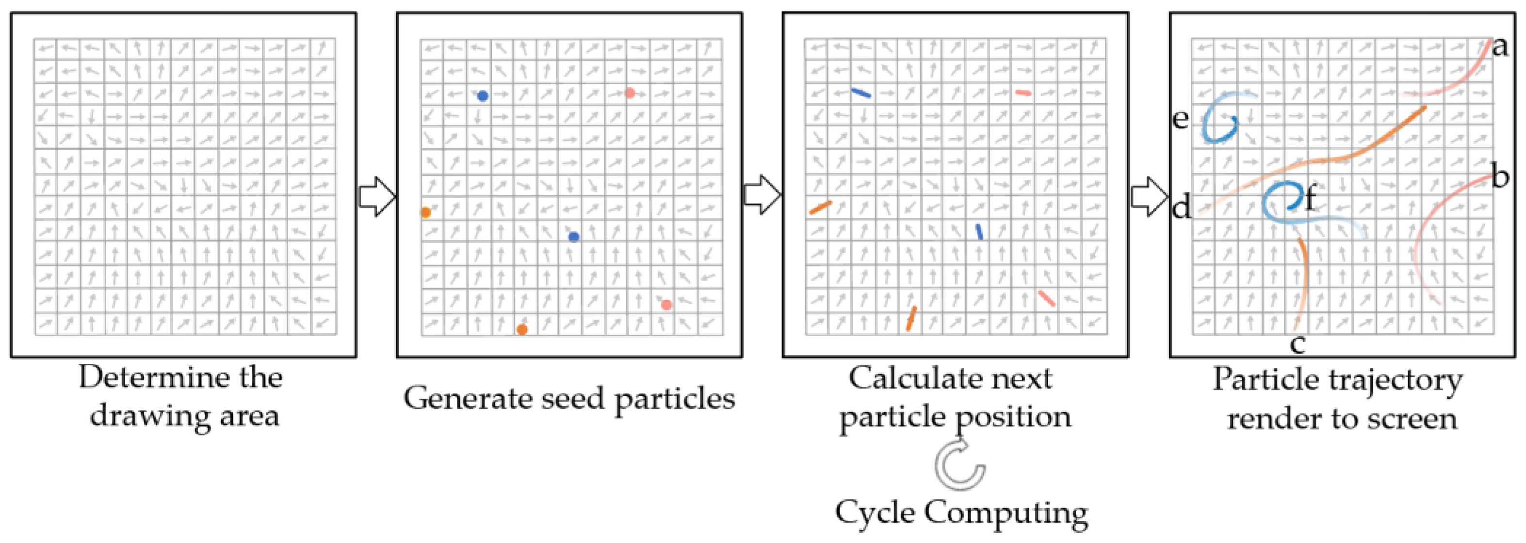
2.3.2. Particle Trajectory Tracking Method Based on Lagrangian Field

The Lagrangian wind field can be used to discover the velocity variation of a single abstract particle with time in the spatial position. The time-varying characteristics of the wind field require a series of particles with a life cycle using continuous wind field data to drive particles for dynamic simulation. The parameters of the wind field particle system mainly include the number, position, velocity, size, color, brightness, transparency, shape, and life cycle of the particles. Some properties of the wind field and the state changes of the particles themselves can be visually represented by the changes in the properties of the particles. The velocity can be mapped by the color properties of the particles, and the life cycle can be reflected by changing the transparency of the particles.

The particle system manager (Figure 4) is an abstract class, consisting of several main components: seeding, symbol designing, particle tracking, rendering, and particle management container. The drawing area is calculated from the wind data and the viewport. The middle rectangle represents the process of the particle system, which is executed on the CPU and GPU. The rendering result is output to the screen. The particle management container also defines two collections: particle collection and WebGL-based drawing command collection. WebGL (Web Graphics Library) is a JavaScript API for rendering high-performance interactive 3D and 2D graphics within any compatible web browser without the use of plugins. The entire rendering process of the particle tracking is realized by using shaders on GPU.

The wind field particle management container manages a collection of particles. Each particle is an abstract expression of the wind field particle, with attributes such as position, acceleration, velocity, direction, color, length, and lifetime. The particle dynamic visualization process is shown in Figure 5. The entire process consists of two parts: data preparation and particle tracking. The blue rectangles represent the processing steps in the workflow and the green diamonds represent the judgement conditions. The detail steps include the following:

(1)

Initialize particles. The wind field state can be obtained by reading the texture data in the current timestamp. A certain number of particles are generated based on the seeding strategy, with initial attributes such as position, velocity, direction, color, and so on. Then, we can use the particle management container to manage the particle collection.

(2)

Parallel particle tracking. We adopt the parallel particle trajectory tracking algorithm to improve the visualization method of the time-varying wind field based on the particle system. The dynamic change in the time-varying wind field is vividly visualized by particle motion in animation form. The spatial position of the particles at different times will produce different velocity changes, which dynamically reflects the velocity and direction of wind field. The particle tracking algorithm calculates the particle trajectory through the integral method (Equation (4)) according to the position and velocity function of the particle.

$$y_{t+\mathsf{\Delta }t}=y_t+{\displaystyle \int v(y_t)}dt$$

(4)

In order to make the particle tracking trajectory smoother, this study adopts the fourth-order Runge–Kutta method (Equation (5)).

$$\left\{\begin{array}{l}{y}_{t+\mathsf{\Delta }t}=y_t+\frac{1}{6}(k_1+2k_2+2k_3+k_4)\\ k_1=v(y_t)\mathsf{\Delta }t\\ k_2=v(y_t+\frac{k_1}{2})\mathsf{\Delta }t\\ k_3=v(y_t+\frac{k_2}{2})\mathsf{\Delta }t\\ k_4=v(y_t+k_3)\mathsf{\Delta }t\end{array}\right.$$

(5)

In Equations (4) and (5), $y$ is the spatial position of the particle, $v\left(y_t\right)$ is the velocity function of the particle at time $t$, $\mathsf{\Delta }t$ is the time interval, and the velocity function of the particle is determined by the spatial position of the particle and the time factor. According to the initial position of the particle, a continuous particle trajectory can be obtained by using the numerical integration method for trajectory tracking. The tracking results of the trajectory line are determined by the efficiency and calculation accuracy of the numerical integration algorithm. In this study, the Runge–Kutta method is selected in the integral algorithm.

(3)

Update the particle property state. The position and color attributes of the particle are updated according to its dynamic attributes, such as speed. In the process of tracking, the particle color is determined by the velocity, the transparency by the lifetime value state, and the spatial position by the particle position in the previous frame, the velocity function, and the time interval defined in both frames.

(4)

Particle rendering. The final performance of visual rendering is reflected by the frame rate, and the factors affecting the performance in the particle system include particle number, data size, and integration algorithm. We improve the performance of the particle system redrawing by establishing a cache on the GPU to exchange and calculate the particle state texture.

(5)

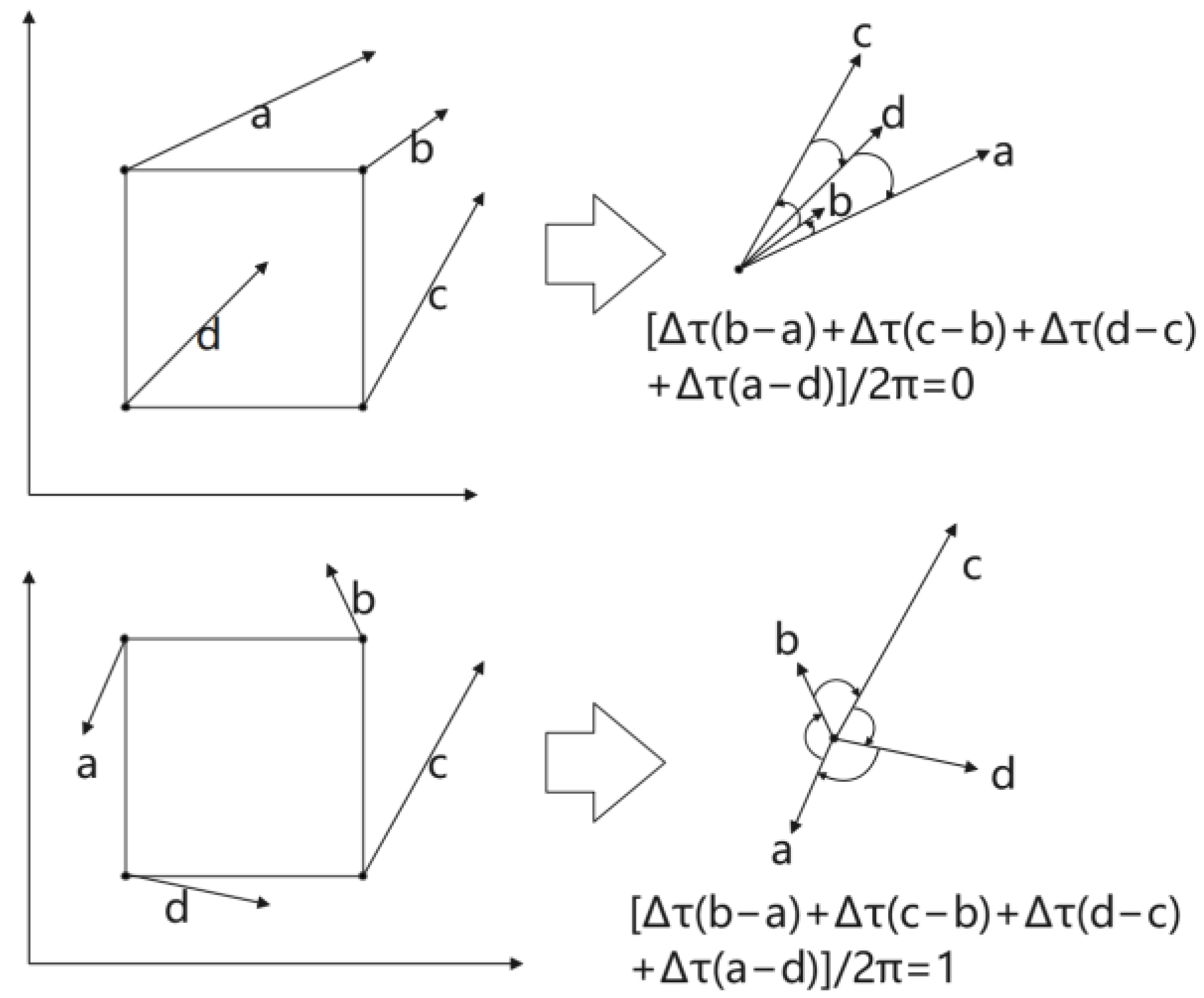
Remove dead particles. The generation of particle trajectories is an iterative calculation process in which the end time of the particle life cycle should be defined. We design the judgment condition for the lifetime to exceed the threshold or for the particle to be tracked to the boundary region or the critical region (the region of velocity 0). In general, if the life cycle ends, it should be removed from the management container. For better scheduling of memory resources, here, we set the transparency of the dead particle to 0 and remove them completely instead. The particle object is kept in the management container and the trajectory is redrawn at the new location, avoiding the repeated scheduling of memory resources for additions and deletions and improving the visualization efficiency.

As shown in Figure 6, the drawing area needs to be defined before particle rendering, which is often determined by the original wind field and the viewable field of the screen. In Figure 6, we use a grid and vector arrows to illustrate the drawing area. Secondly, a large number of random particle objects are generated as alternative seed point sets, and then integral tracking is carried out on them to generate streamline. Finally, we sort out the judgment conditions for stopping integration, which mainly include the following conditions: (1) particle direction beyond the drawing region boundary stops tracking, as shown in path line a and b; (2) the particle life cycle approaches the set life cycle threshold and collides with other particles, which needs to be stopped, as shown in path line c and d; and (3) the step length of the integral line tends to 0, and may cause self-intersecting, generating ring lines, as shown in path line e and f.

The tracking algorithm determines the trajectory accuracy, but the pattern style determines the visualization effect. The color is one of the most active visual variables in visual expression. By assigning color variables to dynamic particles and representing wind field intensity through color mapping, the wind speed scalar value can be displayed intuitively. The color mapping rule is usually set as a function mapping relationship, which determines the effect of drawing to a certain extent. The most common mapping relationship is linear mapping.

Nonetheless, the wind field in the actual scene is complex and changeable, and the numerical distribution of wind speed is uneven. The velocity values are concentrated in a small range, and the characteristics of the velocity values in the region of interest are not prominent enough. Thus, when linear color mapping is used to draw and express the wind field, a continuous large area of low-speed color concentration often appears, which makes it difficult for human eyes to distinguish the wind field information and poses challenges for the extraction of interesting feature regions.

In order to solve the problem caused by linear color mapping, Zhan [24] proposed a nonlinear color mapping scheme based on nonlinear function. The calculation formula is as follows:

$$S_{new}=\frac{L^S-1}{L-1}$$

(6)

In Equation (6), $L$ is a nonlinear mapping factor, $S$ represents the normalized vector value, and $S_{new}$ represents the vector value after nonlinear mapping.

The color mapping method based on nonlinear function can map some more densely distributed wind speed values to more color ranges compared to linear color mapping, which significantly improves the visualization effect. However, the nonlinear function approach requires users to manually specify the mapping factor parameter, the choice of which has a significant impact on the final effect. When one is unfamiliar with the velocity distribution pattern in the vector field, the selection process of the mapping factor parameters becomes tough.

This paper adopts the standard deviation stretching function to realize the mapping of wind speed value to particle symbol color. The standard deviation of the wind speed is calculated with Equation (7).

$$SD=\sqrt{\frac{1}{n}{\displaystyle \sum _{i=1}^n{(x_i-u)}^2}}$$

(7)

where $n$ is the total number of data points and $u$ is the mean.

$$\left\{\begin{array}{c}{U}_{\min }=u-t\times SD\\ U_{\max }=u+t\times SD\end{array}\right.$$

(8)

$$\left\{\begin{array}{c}k=\frac{S_{\max }-S_{\min }}{U_{\max }-U_{\min }}\\ b=\frac{U_{\max }\times S_{\min }-U_{\min }\times S_{\max }}{U_{\max }-U_{\min }}\end{array}\right.$$

(9)

$$S_{new}=\left\{\begin{array}{c}{S}_{\min }\\ k\ast S+b\\ S_{\max }\end{array}\right.\begin{array}{l}where k\times S+b<S_{\min } or S<U_{\min }\hfill \\ where S_{\min }\le k\times S+b\le S_{\max }\hfill \\ where k\times S+b>S_{\max } or S<U_{\max }\hfill \end{array}$$

(10)

In Equation (8), $U_{min}, U_{max}$ mean the value range of the color map and $t$ is the set standard deviation multiple. When $t$ is equal to 2, the standard deviation of the wind speed value is stretched, and the new stretched wind speed effect is obtained through color mapping in Equations (9) and (10). In Equation (9), $S_{max },S_{min }$ represent the maximum and minimum value of the wind speed and $k,b_{ }$ are the slope and intercept of standard deviation stretching function. In Equation (10), $S_{new}$ is the result of the standard deviation stretching of the velocity value.

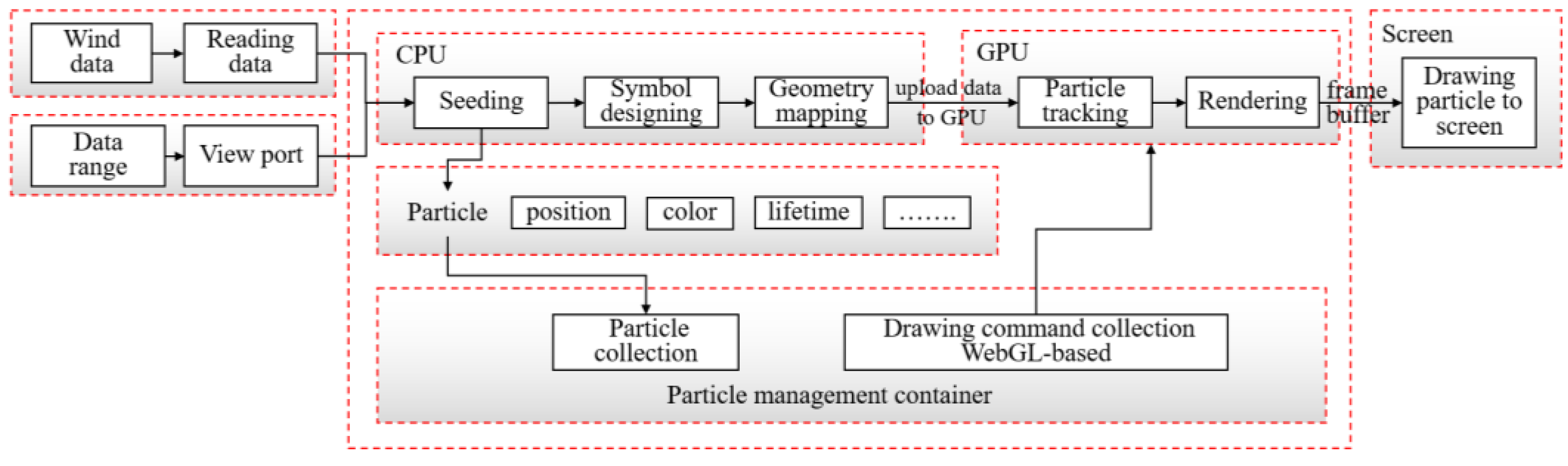
2.3.3. Wind Field Particle Rendering Based on GPU Acceleration

To optimize the dynamic rendering process, we propose a calculation method combining data parallelism and task parallelism, and use GPU parallel computation to improve the tracking and rendering performance of massive particles.

Data parallelism: The basic idea is that the movement of wind field particles is driven by vector field data and stored in a texture, and each particle is divided into a process. Since texture computation in GPU is parallel, the position and lifetime of each particle are updated in parallel and do not affect each other. The particle state is recorded in the position texture and lifetime texture.

Task parallelism: Each particle is regarded as a computing task in particle trajectory tracking, then the entire computing task is divided into different subtasks, such as computing speed and updating position by using the divide-and-conquer strategy. Our strategy can be described as that it is unnecessary to use numerical integration to calculate all the positions of the streamline for one-time rendering in particle trajectory tracking rendering, and the whole streamline rendering process can be divided into continuous subtasks. During GPU calculation, each process calculates particle tracking subtasks independently, and the entire task process is handled by combining different processes ultimately.

The dynamic process of rendering particles based on WebGL is shown in Figure 7, which is divided into wind texture data mapping, parallel particle tracking, and particle graphics rendering. The parallel particle tracking part completes the particle position calculation and motion process inside the shader by rendering to a texture, buffer swapping, and other technical schemes. The particle graphics render uses the frame buffer architectures and the divide-and-conquer method to achieve the rendering of particles.

3. Experiments and Results

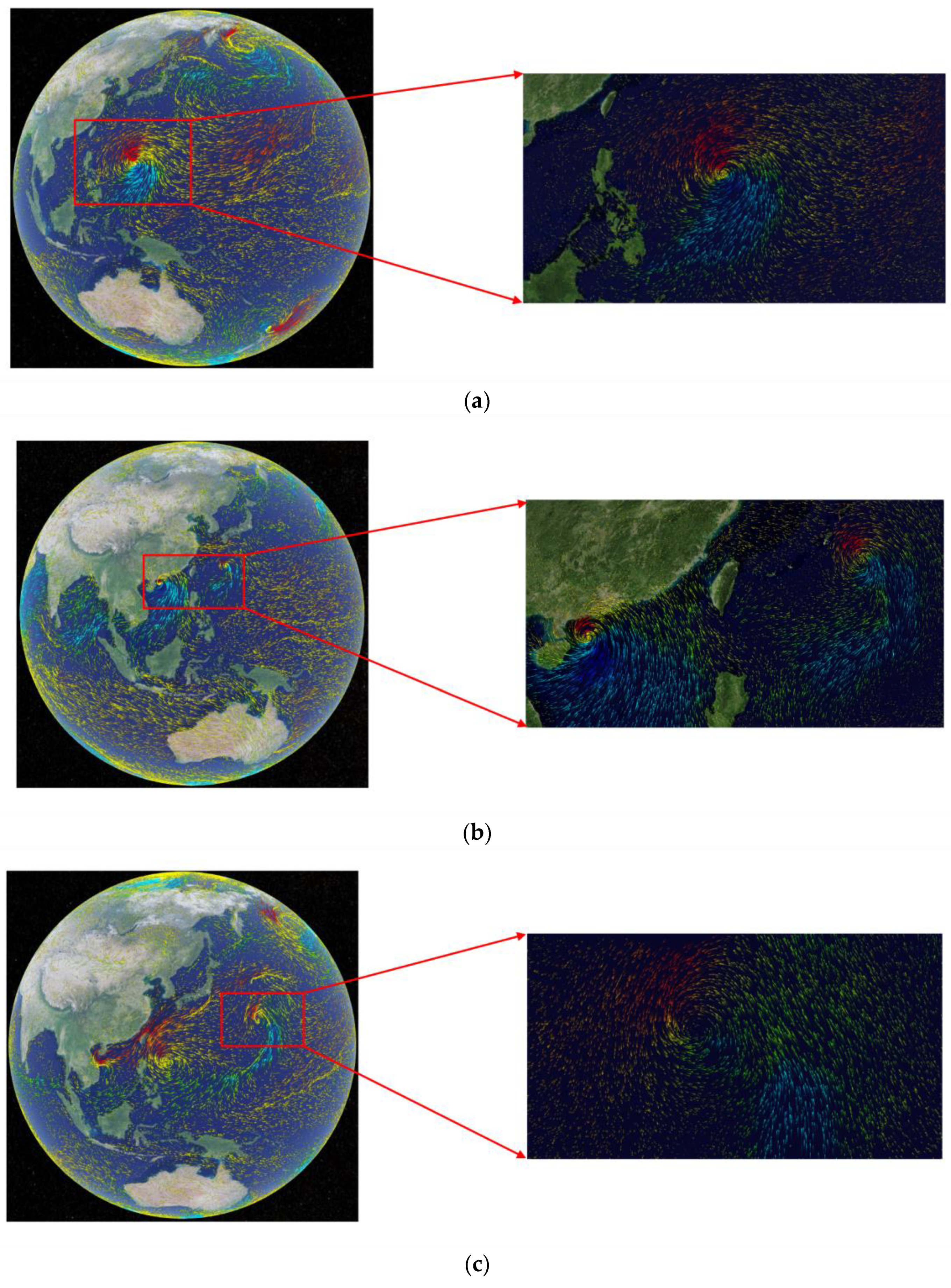
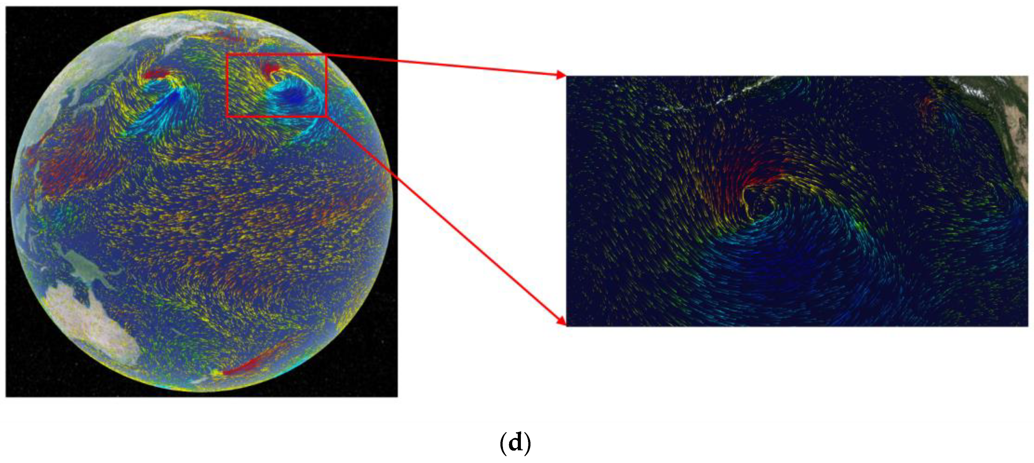
We take the global wind vector field as the research object based on the above method system and realize the dynamic visualization of time-varying wind on the 3D virtual Earth simulation platform based on WebGL. Its major implementation steps are as follows:

(1)

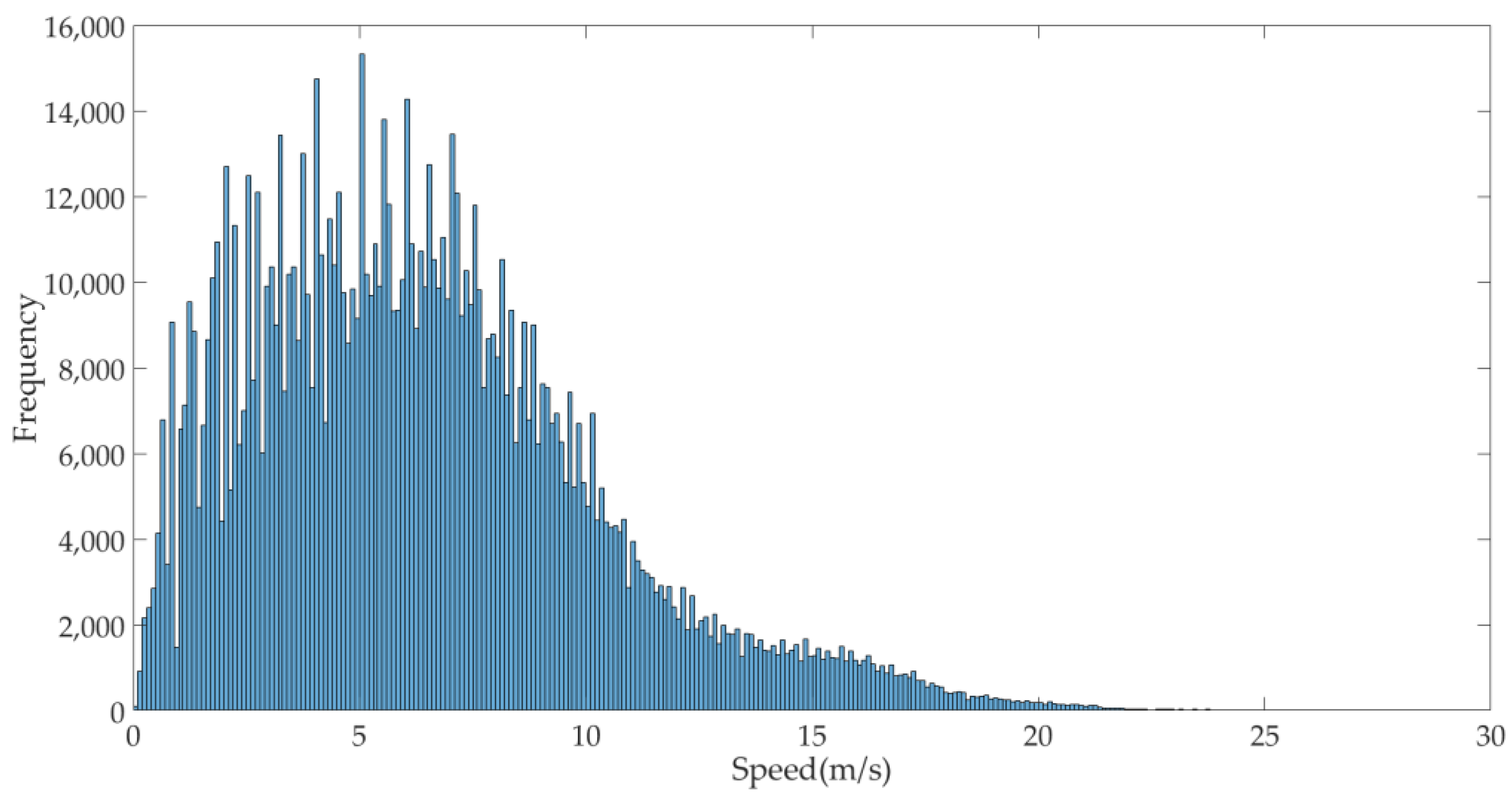
The NetCDF data of the original wind field in the global region are converted into texture data by the preprocessor and the distribution of the global wind speed field is obtained through the mathematical statistics method.

(2)

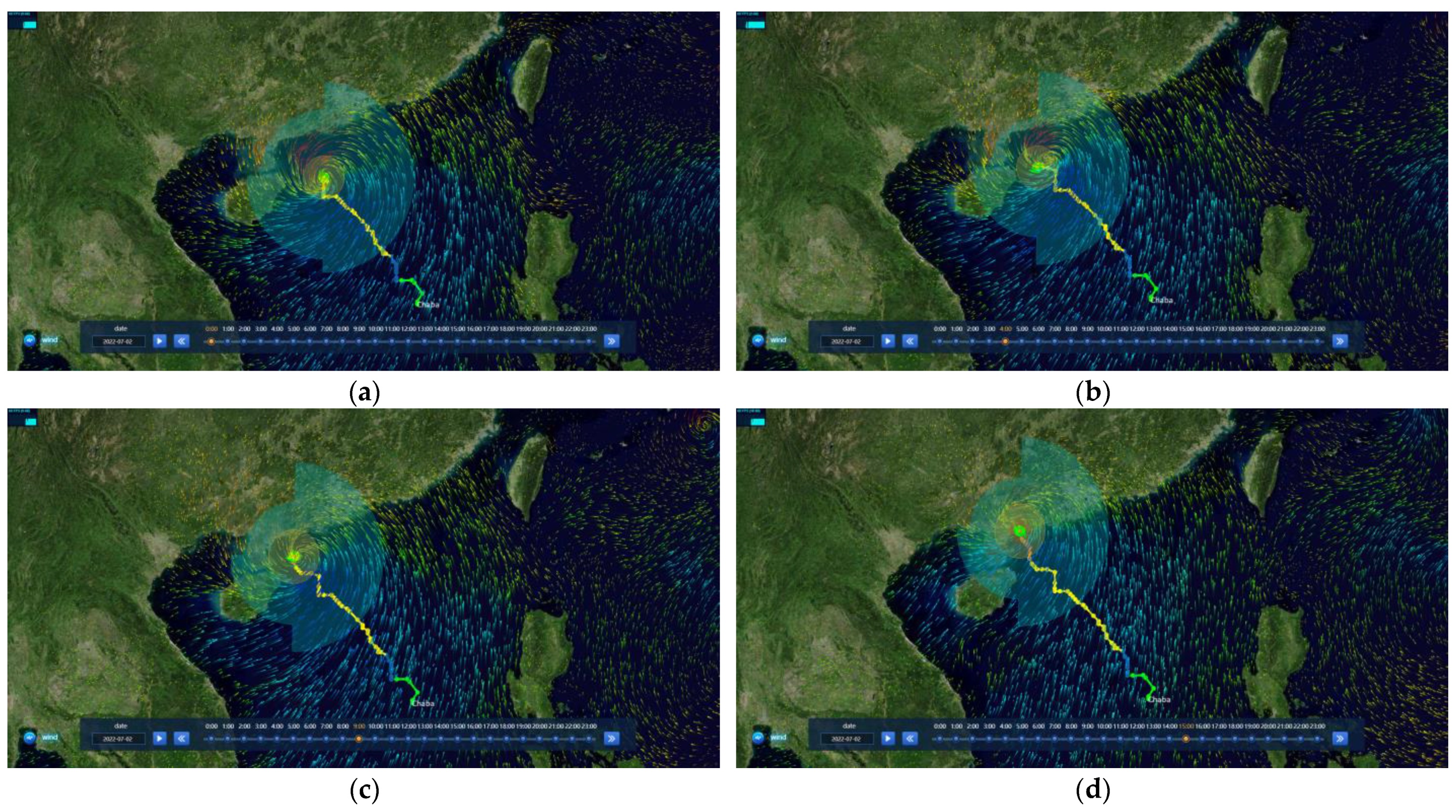
The spatio-temporal linear interpolation algorithm is used for continuous time-series wind data to generate finer data of time-varying wind. The seeding algorithm generates a large number of random particle points with life cycles, and computes the position and velocity of each particle point according to the wind data.

(3)

Finally, the particle system is used to express the wind vector field, the JavaScript scripting language is used to call the WebGL command, and the rendering is performed in the browser to simulate the wind particle trajectory.

The general interpolation algorithms include nearest neighbor interpolation, bilinear interpolation, bicubic interpolation, and so on [25,26]. Figure 8 shows the interpolation algorithms for nearest neighbor interpolation, cubic spline interpolation, and improved bilinear interpolation. The red vector arrows indicate the direction of the sampling point.

We carried out three interpolation comparison experiments on the wind field data. The interpolation results are shown in Figure 8. The nearest neighbor interpolation is efficient, but the interpolation result is poor in data continuity. The cubic spline interpolation and bilinear interpolation guarantee the continuity and the overall effect of the interpolation results. However, the cubic spline interpolation algorithm is more complex than nearest neighbor interpolation and bilinear interpolation, which decreases the efficiency somewhat. The bilinear interpolation algorithm is adopted considering both the efficiency and interpolation results comprehensively.

Figure 9 shows the global wind field distribution statistics at 12:00 on 2 July. It shows that the frequency of the speed distribution is inhomogeneous, similar to Weber distribution, and the frequency of the part with the wind speed greater than 20 m/s is much lower than the other parts. The experiments were carried out on the wind field using linear mapping, nonlinear mapping ($L=1.5$), nonlinear mapping ($L=0.5$), and nonlinear mapping methods based on the double standard deviation, respectively. The experimental results are shown in Figure 10, where the colors range from red to green for drawing.

As shown in Figure 10, we can find that the stretching with double standard deviation has a better effect on color mapping the wind vector field through the comparison experiment of multiple sets of global wind field grid data with a resolution of 1440 × 720 pixels. The color stretching algorithm (Equation (6)) has an unstable factor of parameter L, which requires several experiments to determine, and the expression effect is far less intuitive than the color stretching method based on double standard deviation. The standard deviation mapping function is more suitable for the global wind field characteristics, which can show critical information and obtain better mapping visual effects.

In this paper, the wind field particles are visualized in the global-scale three-dimensional scene using the continuous time series global wind vector field data, and the particles are managed by the particle management container to control their tracking step, life value, state attribute, etc. The spatio-temporal linear interpolation method is used to calculate the position of the next moment in the spatial position of the particle at the current moment and update it in the particle management container, and the life value will be reduced accordingly. When the life value exceeds the life cycle threshold, this particle should be marked as a dead particle and updated, and the continuous trajectory based on the particle tracking algorithm is dynamically drawn on the screen. In order to avoid particles being too concentrated or too sparse, a density control strategy is introduced to adjust the distribution of particles in real time. The number of particles should be appropriately increased in the blank area when the density is less than the threshold. The particle opacity or the number of particles should be appropriately reduced in the high-density area when the density is less than the threshold. It is necessary to control the particle density to obtain good visualization results. According to this strategy, some particles should be eliminated in areas where the particles are too concentrated, so that the number of particles can be kept at an appropriate interval. The visualization effect of the continuous time-varying wind vector field is shown in Figure 11.

Figure 11a–d are the corresponding wind fields at 0:00, 4:00, 9:00, and 15:00 on 2 July. Figure 11 shows the particle visualization effect of continuous dynamic time-varying wind vector field. The redder the color, the faster the speed, and the bluer the color, the slower the speed. This intuitively shows the distribution of the global wind vector field at different times and the evolution trend of the wind field. The particles intuitively characterize the direction and speed of wind field movement. The typhoon Chaba track data are derived from the South China Sea Information Center of State Oceanic Administration. Under the influence of super typhoon Chaba, it rotates counterclockwise with the typhoon eye as the center, and the overall trajectory of the typhoon shows a flow trend from southeast to northwest. The distribution of the wind vector field at the global scale is simulated objectively through experimental analysis. The experimental results conform to the distribution characteristics of the global wind vector field. Compared with geometric visualization methods based on streamlines or the particle system and well-known wind field data visualization projects, such as the windy system (url: embed.windy.com [27], accessed on 1 January 2023) and the earth system (url: earth.nullschool.net [28], accessed on 1 January 2023), the cognitive efficiency of the dynamic map based on the particle system is higher, the cognitive depth and dimension are wider, and the cognitive mode is more similar to the human perception of the real Earth environment. It can obtain the speed and characteristic field of the wind field more intuitively, which is valuable in application for the exploratory analysis of the wind vector field.

The comparison results are shown in Figure 12 when viewing the globe at 4000 km and 500 km and setting the particle number to 10,000, 20,000 and 50,000. It is difficult to display full detail when the particle number is about 10,000 (Figure 12a). The characteristics and motion process of the wind field can hardly be observed when the particle number is about 50,000 (Figure 12c). The display becomes very dense and disturbs the observation of the wind movement process when the particle number is large. The feature and evolution are clear and concise when the particle number is set to about 20,000.

The human vision perception of particle density is different under the conditions of different viewing distances and different particle numbers. It is difficult to observe the distribution characteristics of the scene when the number of particles is too small or too large. The characteristics and evolution are clear and easy to inspect when the number of particles is set to a medium number. The results accord with most human vision habits in this case when the number of particles is set to about 20,000.

We used global wind field data over four seasons to verify the applicability of the experimental results. The wind data are from 12 April, 2 July, 14 October 2022, and 10 January 2023. As shown in Figure 13, the results show that the proposed method can depict the details of the wind field well. The colors are the result of speed mapping, fading from red to blue. The redder the color, the faster the speed, while the bluer the color, the slower the speed.

The prototype system was developed based on the framework of the three-dimensional virtual Earth visualization simulation platform. The client computer is configured with 4 GB for memory and 2 GB for the independent graphics card, and the Chrome browser supporting WebGL engine is installed. The average frame rate of the system is maintained at around 40 frames per second, satisfying visual effects and smooth experience requirements for users.

Efficiency verification is shown in Figure 14; the visualization frame rate decreases as the view distance and particle number increase. Human vision can perceive a frame rate of 24 frames per second when comfortable and relaxed. The dynamic picture will be smooth when the frame rate of rendering reaches about 60 FPS. Generally, the higher the frame rate, the smoother the visual perception, and the smoother the expression of the particle system. The rendering frame rate can be maintained at more than 40 frames when the number of particles reaches about 150,000, which can still meet the needs of smooth visual perception of human vision and provide smooth animation effects for most users. In addition, this paper also conducts rendering frame rate experiments under different view distances. The view distance is set at 1000 km, 2000 km, and 3000 km, respectively. The results shows that the rendering efficiency continues to decline with the increase in viewing distance. The minimum frame rate is 45 FPS when the number of particles is 160,000 and the view distance is 3000 km.

4. Conclusions and Future Work

This paper proposes a dynamic visualization method of spatiotemporal wind fields based on the particle system. The characteristics of the time-varying wind field are effectively represented on the Digital Earth platform. The contribution of this paper is as follows:

(1)

Firstly, the linear interpolation algorithm is used to carry out fine interpolation for the original continuous sequential wind field data according to the consecutive wind field data of adjacent moments, and the multi-time wind field is mapped to the dense texture, which makes it convenient for WebGL and GPU to process and exchange data.

(2)

Secondly, the particle motion rules of vector wind field are explored based on the Lagrangian method, and the fourth-order Runge–Kutta method is used to construct a smooth wind field visualization.

(3)

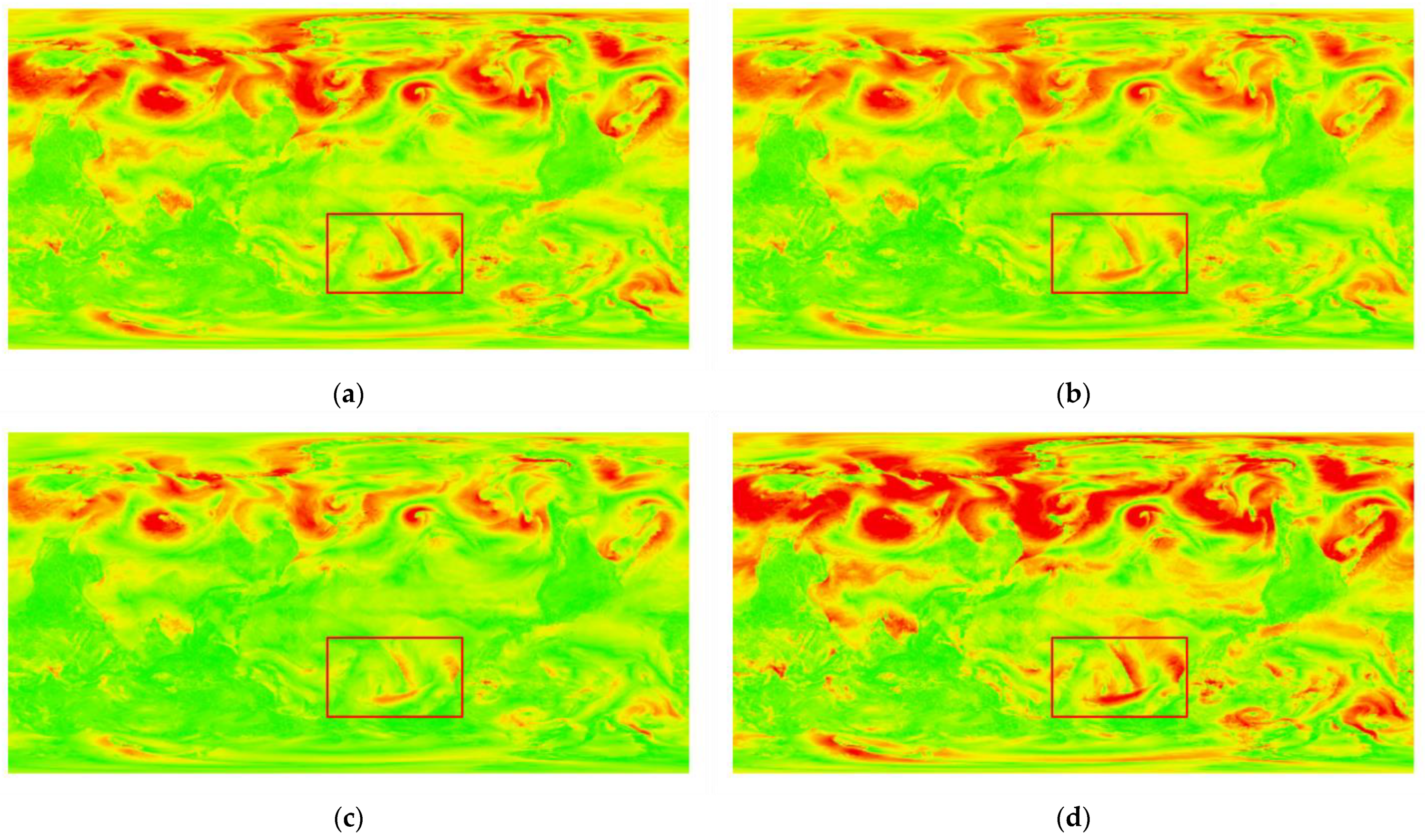
Thirdly, we adopt a nonlinear mapping method based on double standard deviation to improve the color representation of wind field features. The adaptive symbolization scheme for intensity distribution characteristics of the global wind vector field utilizing mathematical statistics can prominently reflect the vector field information.

In this paper, we realized the visualization of a continuous time-varying wind vector field and particle system based on the three-dimensional virtual Earth simulation platform. The interpolation algorithms build detailed driving data for particle system visualization. The Lagrangian-based tracking algorithm smooths the particle trajectory. The color stretching method based on double standard deviation enhances the visual experience. The experimental results show that the continuous dynamic visualization method of the global time-varying wind vector field based on particle system can accurately and vividly represent the dynamic evolution details of the wind vector field driven by the time factor and show a more realistic time-varying wind field visualization effect in the three-dimensional virtual Earth scene to intuitively express the spatio-temporal evolution process of the vector wind field. This study has great value and significant reference for the study and analysis of dynamic visualization of global meteorological information.

There are still some defects in this study. The color mapping is calculated based on nonlinear function after mathematical statistics. In addition, other attributes of particles, such as particle number and life cycle, need to be compared through experience or several experiments to obtain relevant optimal solution parameters, which is inconvenient for users, increases the difficulty of user perception for wind field, and puts forward higher professional requirements for users. We should consider quantizing parameters such as map load rate and other hardware parameters, and dynamic improvement of parameter settings to further improve the quality of visualization.

In future work, we will further analyze the causes of wind field changes, explore the spatial distribution of wind field features, efficiently extract the feature regions of interest, and construct a multi-scale feature model based on global wind field. On this basis, we will realize a multi-scale three-dimensional dynamic visualization platform capable of real-time analysis and feature expression to simulate wind field. The study of visualization for wind field can aid in planning for ship navigation and forecasting for typhoons and cyclones, which is significant to human production and life. The visualization simulation of wind field is carried out to provide support for wind prevention and disaster reduction.

References

1. Shi, L. Lagrangian-Based Simplification and Feature Estimation for Flow Visualization. Ph.D. Thesis, University of Houston, Houston, TX, USA, 2019. [Google Scholar]
2. Laidlaw, D.H.; Kirby, R.M.; Jackson, C.D.; Davidson, J.S.; Miller, T.S.; da Silva, M.; Warren, W.H.; Tarr, M.J. Comparing 2D vector field visualization methods: A user study. IEEE Trans. Vis. Comput. Graph. 2005, 11, 59–70. [Google Scholar] [CrossRef] [PubMed]
3. Ware, C.; Kelley, J.G.W.; Pilar, D. Improving the Display of Wind Patterns and Ocean Currents. Bull. Am. Meteorol. Soc. 2014, 95, 1573–1581. [Google Scholar] [CrossRef]
4. Fang, Y.; Ai, B.; Fang, J.; Xin, W.; Zhao, X.; Lv, G. Multi-Scale Flow Field Mapping Method Based on Real-Time Feature Streamlines. ISPRS Int. J. Geo-Inf. 2019, 8, 335. [Google Scholar] [CrossRef] [Green Version]
5. Wu, K.; Liu, Z.; Zhang, S.; Moorhead Ii, R.J. Topology-aware evenly spaced streamline placement. IEEE Trans. Vis. Comput. Graph. 2010, 16, 791–801. [Google Scholar] [CrossRef] [PubMed]
6. Huang, J.; Pan, Z.; Chen, G.; Chen, W.; Bao, H. Image-space texture-based output-coherent surface flow visualization. IEEE Trans. Vis. Comput. Graph. 2013, 19, 1476–1487. [Google Scholar] [CrossRef] [PubMed]
7. Reeves, W.T. Particle Systems—A Technique for Modeling a Class of Fuzzy Objects. ACM Trans. Graph. 1983, 2, 91–108. [Google Scholar] [CrossRef] [Green Version]
8. Kruger, J.; Kipfer, P.; Kondratieva, P.; Westermann, R. A particle system for interactive visualization of 3D flows. IEEE Trans. Vis. Comput. Graph. 2005, 11, 744–756. [Google Scholar] [CrossRef] [PubMed]
9. Chen, C.; Yan, S.; Yu, H.; Max, N.; Ma, K. An Illustrative Visualization Framework for 3D Vector Fields. Comput. Graph. Forum 2011, 30, 1941–1951. [Google Scholar] [CrossRef] [Green Version]
10. Joshi, A.; Rheingans, P. Illustration-inspired techniques for visualizing time-varying data. In Proceedings of the VIS 05. IEEE Visualization, Minneapolis, MN, USA, 23–28 October 2005; pp. 679–686. [Google Scholar] [CrossRef]
11. Hou, X. Research on visualization method of 3D time-varying flow field with LIC algorithm. Comput. Era 2020, 7, 86–89. [Google Scholar] [CrossRef]
12. Hu, Z.; Liu, P.; Gong, J.; Wang, Q. Design and Implementation of Multidimensional and Animated Visualization System for Typhoon on Virtual Globes. Geomat. Inf. Sci. Wuhan Univ. 2015, 40, 1299–1305. [Google Scholar] [CrossRef]
13. Liu, P.; Gong, J.; Yu, M. Visualizing and analyzing dynamic meteorological data with virtual globes: A case study of tropical cyclones. Environ. Model. Softw. 2015, 64, 80–93. [Google Scholar] [CrossRef]
14. Mei, H.; Chen, H.; Zhao, X.; Liu, H.; Zhu, B.; Chen, W. Visualization System of 3D Global Scale Meteorological Data. J. Softw. 2016, 27, 1140–1150. [Google Scholar] [CrossRef]
15. Pirotti, F.; Brovelli, M.A.; Prestifilippo, G.; Zamboni, G.; Kilsedar, C.E.; Piragnolo, M.; Hogan, P. An open source virtual globe rendering engine for 3D applications: NASA World Wind. Open Geospat. Data Softw. Stand. 2017, 2, 4. [Google Scholar] [CrossRef] [Green Version]
16. Liu, H. Method of Web Digital Earth Ocean Vector Field Data Dynamic Visualization Based on the Particle System. Master’s Thesis, Chinese Academy of Sciences (Institute of Remote Sensing and Digital Earth), Beijing, China, 2017. [Google Scholar]
17. Tan, J.; Wang, S.; Guo, C. Video formatting method of near-space data for Web scientific visualization. J. Beijing Univ. Aeronaut. Astronaut. 2020, 46, 712–723. [Google Scholar] [CrossRef]
18. Wang, S.; Li, W. Capturing the dance of the earth: PolarGlobe: Real-time scientific visualization of vector field data to support climate science. Comput. Environ. Urban Syst. 2019, 77, 101352. [Google Scholar] [CrossRef]
19. Yao, A.; Wang, L.; Li, J.; Xia, X.; Jin, X.; Jing, N. 2D/3D Visualization of Large-Scale Wind Field based on WebGL. In Proceedings of the 2020 International Conference on Aviation Safety and Information Technology, Weihai, China, 14–16 October 2020; pp. 269–274. [Google Scholar]
20. Chandler, J.; Obermaier, H.; Joy, K.I. Interpolation-Based Pathline Tracing in Particle-Based Flow Visualization. IEEE Trans. Vis. Comput. Graph. 2015, 21, 68–80. [Google Scholar] [CrossRef] [PubMed]
21. Li, W.; Wang, S. PolarGlobe: A web-wide virtual globe system for visualizing multidimensional, time-varying, big climate data. Int. J. Geogr. Inf. Sci. 2017, 31, 1562–1582. [Google Scholar] [CrossRef]
22. Helman, J.L.; Hesselink, L. Visualizing vector field topology in fluid flows. IEEE Comput. Graph. Appl. 1991, 11, 36–46. [Google Scholar] [CrossRef]
23. Mann, S.; Rockwood, A. Computing singularities of 3D vector fields with geometric algebra. In Proceedings of the IEEE Visualization, 2002. VIS 2002, Boston, MA, USA, 27 October–1 November 2002; pp. 283–289. [Google Scholar]
24. Zhan, F.; Hu, W.; Yuan, G. Improvement of 2D LIC Algorithm for Vector Field Visualization. Comput. Sci. 2013, 40, 257–261. [Google Scholar]
25. Deng, C. Research of Image Interpolation Algorithm. Master’s Theses, Chongqing University, Chongqing, China, 2011. [Google Scholar]
26. Ding, X. Research and comparison of Matlab interpolation algorithm for image scaling function. J. Hubei Univ. (Nat. Sci.) 2018, 40, 396–400+406. [Google Scholar]
27. Windy: Wind Map & Weather Forecast. Available online: https://embed.windy.com/ (accessed on 1 January 2023).
28. Earth: A Global Map of Wind, Weather, and Ocean Conditions. Available online: https://earth.nullschool.net/#current/wind/surface/level (accessed on 1 January 2023).
Figure 1. Overview diagram for spatio-temporal dynamic visualization based on particle system.
Ijgi 12 00146 g001
Figure 2. Schematic of wind field interpolation.
Ijgi 12 00146 g002
Figure 3. The sum index of angle difference schematic.
Ijgi 12 00146 g003
Figure 4. The diagram of the particle system manager structure.
Ijgi 12 00146 g004
Figure 5. Particle trajectory rendering flow chart.
Ijgi 12 00146 g005
Figure 6. Schematic diagram of particle trace generation.
Ijgi 12 00146 g006
Figure 7. Schematic diagram of WebGL-based particle system.
Ijgi 12 00146 g007
Figure 8. (a) Original wind data rendering result; (b) nearest neighbor interpolation result; (c) cubic spline interpolation result; (d) bilinear interpolation result.
Ijgi 12 00146 g008
Figure 9. Velocity distribution histogram.
Ijgi 12 00146 g009
Figure 10. Color mapping experiment effect. The red areas are the regions with higher velocity and the green areas are the regions with lower velocity. Besides, the red box is the place where rendering effects are compared. (a) Linear color mapping; (b) L = 1.5 , nonlinear mapping; (c) L = 0.5 , nonlinear mapping; (d) color mapping method based on double standard deviation.
Ijgi 12 00146 g010
Figure 11. Wind-based time-varying particle tracking. (a) is the wind field at 0:00 on 2 July 2022. (b) is the wind field at 4:00 on 2 July 2022. (c) is the wind field at 9:00 on 2 July 2022. (d) is the wind field at 15:00 on 2 July 2022.
Ijgi 12 00146 g011
Figure 12. Rendering results at different viewing distances and different particle numbers. The red position is area with fast speed, and blue position is area with slow speed. (a) Rendering result of 10,000 particles at 4000 km; (b) rendering result of 20,000 particles at 4000 km; (c) rendering result of 50,000 particles at 4000 km; (d) rendering result of 10,000 particles at 500 km; (e) rendering result of 20,000 particles at 500 km; (f) rendering result of 50,000 particles at 500 km.
Ijgi 12 00146 g012
Figure 13. (a) Wind experiment result from 12 April 2022; (b) wind experiment result from 2 July 2022; (c) wind experiment result from 14 October 2022; (d) wind experiment result from 10 January 2023.
Ijgi 12 00146 g013aIjgi 12 00146 g013b
Figure 14. Statistics of rendering efficiency at different viewing angles based on frame rate.
Ijgi 12 00146 g014