
Measuring Traffic Congestion with Novel Metrics: A Case Study of Six U.S. Metropolitan Areas

1
Department of Natural Sciences, University of West Georgia, 1601 Maple St., Carrollton, GA 30118, USA
2
Department of Geography, Dongguk University, Seoul 04620, Republic of Korea
3
Department of Geography, Chonnam National University, Gwangju 61186, Republic of Korea
4
Department of Geography, Kyung Hee University, Seoul 02447, Republic of Korea
5
Department of Computing and Mathematics, University of West Georgia, Carrollton, GA 30118, USA
*
Author to whom correspondence should be addressed.
ISPRS Int. J. Geo-Inf. 2023, 12(3), 130; https://doi.org/10.3390/ijgi12030130
Submission received: 14 January 2023
/
Revised: 10 March 2023
/
Accepted: 16 March 2023
/
Published: 20 March 2023
(This article belongs to the Special Issue Urban Geospatial Analytics Based on Crowdsourced Data)
Abstract
:Quantifying traffic congestion is a critical task for transportation planning and research. Numerous metrics have been developed, mainly focusing on changes in vehicle speeds, their extents, and travel time. In this study, new metrics are presented using the Hägerstrand’s space-time cube that has been studied from time geography perspectives since the 1960s. Particularly, the product of distance and time, i.e., distanceTime, is proposed as a base metric to measure traffic congestion amounts. Using the base metric such as mileHours, metrics of weighted congestion and normalized congestion amounts were also developed. New metrics were applied to six metropolitan areas and their vicinities in the United States (Atlanta, Chicago, Washington, D.C. and Baltimore, Dallas and Fort Worth, Los Angeles, and New York), and congestion amounts were calculated and compared. The Google Traffic Layer API was used to obtain traffic congestion datasets for six months (April–September 2022), and GIS (geographic information systems) was used for delineating road features and traffic intensity levels. Among the six areas, New York and its vicinity showed the largest congestion when only heavy congestion was used. Los Angeles and its vicinity showed the largest congestion when all congestion levels were considered. This study shows that the proposed metrics are very effective in summarizing traffic amounts and broadly applicable for further analyses of traffic congestion phenomena by associating various other factors, such as weekdays, months, or gas prices. The new metrics developed in this research may help transportation researchers and practitioners by providing them with a set of metrics applicable to summarizing congestion amounts by synthesizing congestion intensity, extent, and duration.
1. Introduction
Traffic congestion (TC) reflects the difference between the travel time experienced during busy traffic periods and when the road is lightly traveled [1]. TC can be defined as travel time or delay in excess of that normally incurred under light or free-flow travel conditions [2]. The four components of TC include intensity, extent, duration, and reliability, where intensity reflects the severity of congestion typically expressed as a rate, duration refers to the amount of time the travel system is congested, and extent describes the geographic distance of roads that are congested or the number of travelers or vehicles affected by the congestion [1,2].
TC metrics were characterized by twelve distinctive situations based on the relation of three road system types (i.e., single roadway, corridor, and areawide network) and four congestion components (i.e., duration, extent, intensity, and reliability) [2]. For example, the hours that facility operates below acceptable speed was classified as the duration metrics for a single roadway. Interestingly, a set of travel time contour maps or the bandwidth maps showing the amount of congested time for system sections were classified as the duration metrics of an areawide network.
Multiple TC measurement tools have been developed. Afrin and Yodo [3], for example, grouped them into five categories based on the critical properties they represent (note: typical metrics in parentheses)—speed (speed reduction index or speed performance index), travel time (travel rate), delay (delay ratio or delay rate), level of service (volume to capacity ratio), and congestion indices (relative congestion index). In addition, they put congested hours, travel time index, and planning time index into the federal congestion measures used by the U.S. DOT-FHWA.
The TC metrics that are commonly used include travel time index (TTI), vehicle miles traveled (VMT), vehicle hours traveled (VHT), volume capacity (V/C) ratio, and peak traffic period duration (PTPD) [4,5]. TTI compares peak period travel time to free-flow travel time and is typically expressed as a ratio [6]. VMT evaluates the extent of the TC and measures the congested miles in peak hours [7]. The V/C ratio is calculated by dividing the volume of traffic on a roadway by the roadway’s capacity [8,9]. PTPD assesses how many hours are congested daily during morning and evening peak times [4]. As a variant of PTPD, INRIX developed the total number of hours lost (HL) in congestion during peak commute periods compared to off-peak conditions and used HL to measure TC in metropolitan areas and publish annual Global Traffic Scorecards [10].
Even though multiple TC metrics identify individual TC components well, particularly, intensity, extent, and duration, no metrics represent multiple TC components simultaneously, such as intensity with duration or intensity and duration with extent. Therefore, there are no metrics available that may answer simple questions such as “What is the traffic congestion amount in a city?”. Considering that TC is a spatiotemporal phenomenon, wherein certain levels of intensity are inseparable, it is necessary to develop new metrics that synthesize the three TC components or dimensions, i.e., intensity, extent, and duration, intrinsically. This research explores the synthesis of the three TC dimensions from a geographic spatiotemporal perspective. Particularly, research objectives are (1) developing new metrics that incorporate traffic intensity, extent, and duration together, and (2) demonstrating the applicability of the metrics with real-world examples.
To accomplish the objectives, TC intensity, extent, and duration are conceptualized in a space-time cube and synthesized by novel TC metrics, such as distanceTime, weighted distanceTime, and normalized distanceTime (Section 2). Applying the new metrics, Section 3 compares the average daily heavy congestion, average daily weighted congestion, normalized average daily heavy congestion, and normalized average daily weighted congestion among six U.S. metropolitan areas. Then, TCs are compared by weekdays and months and further analyzed in relation to monthly gas price changes. Section 3 also compares metropolitan congestion amounts with the city rankings using the INRIX Scorecard. After a brief discussion about the applicability of the new metrics, Section 4 summarizes this research with conclusions.
2. Materials and Methods
2.1. Space-Time Cube and Traffic Congestion
TC is a physical phenomenon that has the properties of geographic location (i.e., extent) and temporal duration with certain levels of severity (i.e., intensity). Geographic and temporal phenomena have been modeled and researched actively since Hägerstrand introduced the space-time cube (or space-time model) for time geography in the 1960s [11,12,13]. Particularly, recent advancements in geographic information systems (GIS) and location-based services, such as GPS, mobile phones, and radiofrequency identification (RFID), have greatly expanded capabilities for collecting and processing spatiotemporal data with improved analytical methodologies and have opened various opportunities for researching mobility including accessibility [14].
Typical space-time models are composed of the 2-dimensional geographic space along the x and y axes and the time dimension along the z axis [12]. Numerous approaches have been proposed to model the time dimension effectively in GIS environments, and, according to Siabato et al. [15], the snapshot approach has been the most common solution to analyzing spatiotemporal data in GIS. The snapshot approach is based on the field view of geospatial data modeling [16], where real-world phenomena are represented on a continuous field. The raster representations of digital elevation models, land cover maps, aerial photos, and satellite imagery are some examples of the field view representations [17]. Multiple object-based approaches have also been developed actively based on the object view in geospatial data modeling that represents real-world features with a series of discrete objects, such as points, lines, and polygons [16]. Examples of object-based methods include, but are not limited to, object-oriented approaches [18,19,20], event-based approaches [21,22,23], feature-based approaches [24,25,26], and agent-based approaches [27,28,29].
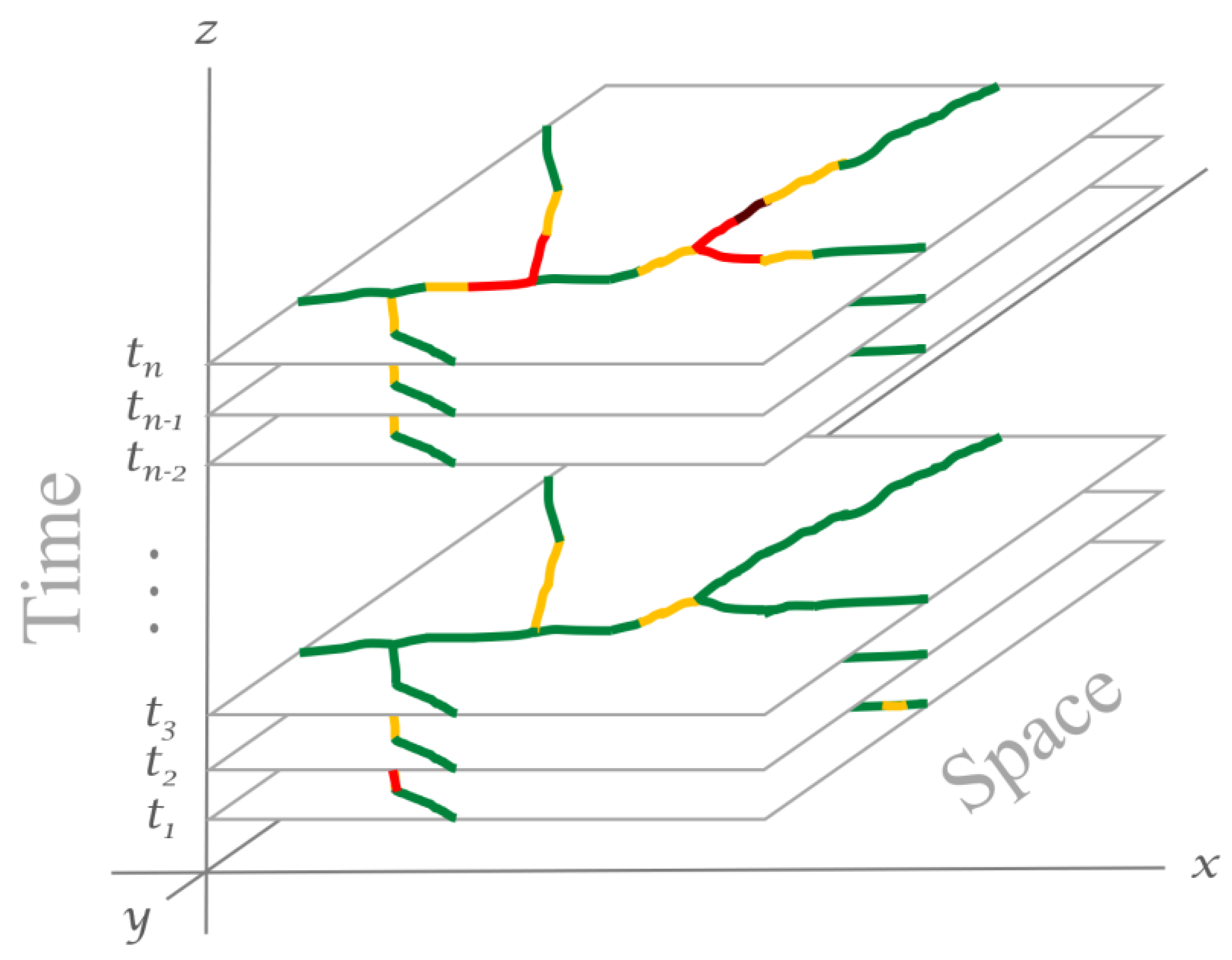
If floating car data (FCD) are available with time-tagged location information, the object-based approaches may be very effective because the continuously changing mobility data of individuals or vehicles can be modeled in the space-time cube as temporal location vectors. On the other hand, if TC intensity maps are collected as temporal slices, they may best fit into a space-time cube as a series of temporal snapshots as shown in Figure 1. Along the temporal axis z, traffic congestion snapshots may be collected at regular intervals, such as every 10 min, every hour, once a day, etc. Congestion snapshots may also be collected at various geographic extents that are scalable from a single spot or a road section to a large metropolitan region.
2.2. Traffic Congestion Metrics from a Space-Time Cube
From a geography perspective, one way of identifying the TC quantity of an area from a snapshot of intensity levels is to calculate the total distance of congestion. As Lomax et al. [2] identified, the percent or miles of congested roads can be calculated from a snapshot in the space-time model. Even though the percent or miles is dependent on how congestion is defined, a simple arithmetic sum of congested sections will identify the TC quantity. For example, a total of 20 miles of heavily congested roads during a morning rush hour in a metropolitan area will give simple and intuitive information about its traffic conditions.
When multiple snapshots along the time axis are accounted, the simple sum of individual distances needs to be refined. In this case, the time domain should be integrated with the geographic domain, and it can be accomplished by multiplying congested road distance and temporal duration. Using time to express the amount of a physical quantity is not new. The multiplication concept has been used in physics frequently. For example, batteries’ electric power capacities have been noted by the Watt-hours unit (or Ampere hour in Ah), which is calculated by multiplying Watt and hours. The same method can be applied to temporal geographic phenomena like TC, as denoted in Equation (1):
where τ is TC amount in distanceTime, d is the total distance of congested roads in a temporal snapshot, and t is the duration of the congestion. For example, if an area (or a road section) experienced 3.2 km of congestion for 3 h, the area experienced a total of 9.6 kmHours of congestion. The 9.6 kmHours can be converted into any other distance and time units; therefore, the 9.6 kmHours are equivalent to 576.0 kmMinutes or 6.0 mileHours. In a real-world situation, the geographic extent of TC varies continuously; therefore, the d value changes dynamically, too. If d values were sampled n times over the temporal duration of t, then the TC amount in distanceTime is the product of the average of d values () and the temporal duration t, as shown in Equation (2):
For example, if d values from three hourly samples are, d = [1.2, 2.6, 5.8] in km over a duration of 3 h, then is 3.2 km and t is 3 h. Multiplying them gives the total TC amount, = 9.6 kmHours. Further, the τ unit, i.e., distanceTime, is different from distance per time. The 9.6 kmHours congestion for 3 h would indicate an average of 3.2 km congestion from the hourly samples.
The distanceTime unit can be represented using various temporal units. For example, if an area experienced an average of 2 km congestion from multiple samples in the span of a month (note: suppose a month is composed of 30 days), the total TC amount (τ) is 2 kmMonths that is equivalent to 60 kmDays or 1440 kmHours. It is also equivalent to 0.16667 kmYears of traffic amount. Even if the time unit in τ can be larger than the sampling period, such extrapolation should be used with caution.
For practical uses of TC metrics, such as comparing TC amounts among multiple cities, it may be necessary to summarize TC amounts (τ) hourly, daily, monthly, or even annually. In this case, it is necessary to set a base unit of distanceTime to work with. Suppose mileHour is used for a base unit, and a city experiences 2 miles of congestion consecutively. Then, the city’s TC amount (τ) is 2 mileHours hourly, 48 mileHours daily, 1440 mileHours monthly, and 17,280 mileHours annually. Once TC amounts are grouped into temporal units, secondary statistics may be derived from them, such as average daily mileHours.
2.3. Weighted Congestion Distance
When calculating traffic congested road distances, a binary, dichotomous delineation of congestion events was assumed so far; however, TC occurs at varying intensity levels in the real world. If intensity levels are available at varying degrees in a road network, congested road distances can be calculated using the intensity levels as weighting values to the distance. Suppose intensity levels (w) range, w = [0.0–1.0], where 0.0 is free-flow condition and 1.0 is full, maximum congestion. Then, the weighted congestion distance is , at each road section. For a regional road network, the total weighted congestion distance in a snapshot is the sum of weighted distances, as Equation (3):
where n is the total road segments in a snapshot, and w is congestion intensity levels ranging from 0.0 to 1.0. Multiple existing metrics for measuring TC intensity may be referenced for weighting values, such as speed reduction index (SRI), volume–capacity ratio, speed performance index, travel rate index, and congestion severity index. Among them, SRI appears to be a good choice because it represents varying speed levels very well on a continuous scale. It was also recommended as the most appropriate congestion measure by Bruwer and Andersen [30]. The SRI represents the ratio of the decline in speeds from free-flow conditions [5]. SRI can be applied to individual freeway segments, entire routes, and even entire urban areas. SRI is calculated as SRI = (1.0—operatingSpeed/freeFlowSpeed) × 10 and ranges from 0 to 10. Without the scalar multiplication of 10, SRI ranges from 0.0 to 1.0, which may work well as weighting values, as in Equation (4):
where w is the congestion weight at a road segment, Sm is the measured speed, and Sf is the free-flow speed. Interestingly, researchers found that congestion occurs when the SRI exceeds 0.4, corresponding to a 40% reduction in speed from free flow, the point at which road users become aware of congestion [2,3,30].
2.4. Normalized Congestion Metrics
When conducting comparisons of TC amounts among multiple places, it is not meaningful to directly compare TC amounts (τ) when the road network distances are significantly different. Such comparisons will only be meaningful after normalizing TC amounts. One way of normalizing TC amounts is to use the maximum congestion amount possible in the network () as the denominator, as shown in Equation (5), where is the product of total road length and the duration of measurement:
For example, suppose cities A and B have congestion amounts of 20 and 300 mileHours for 24 h in a day and the cities’ total road lengths are 50 and 500 miles, respectively. Then, their maximum possible congestion amounts () become 1200 mileHours and 12,000 mileHours, respectively, by multiplying total distance and the duration of 24 h, i.e., 50 × 24 and 500 × 24. The percent congestion amounts of two cities, then, are 1.67% and 2.50%, respectively. Simply comparing the percent values indicates that city B is more congested. Even if the normalized congestion amounts allow for comparisons among cities, they need to be used with caution in real-world applications because significantly different population sizes, road types and capacities, road densities, city densities, and areal sizes may also affect the normalized values.
2.5. Data Collection and Processing
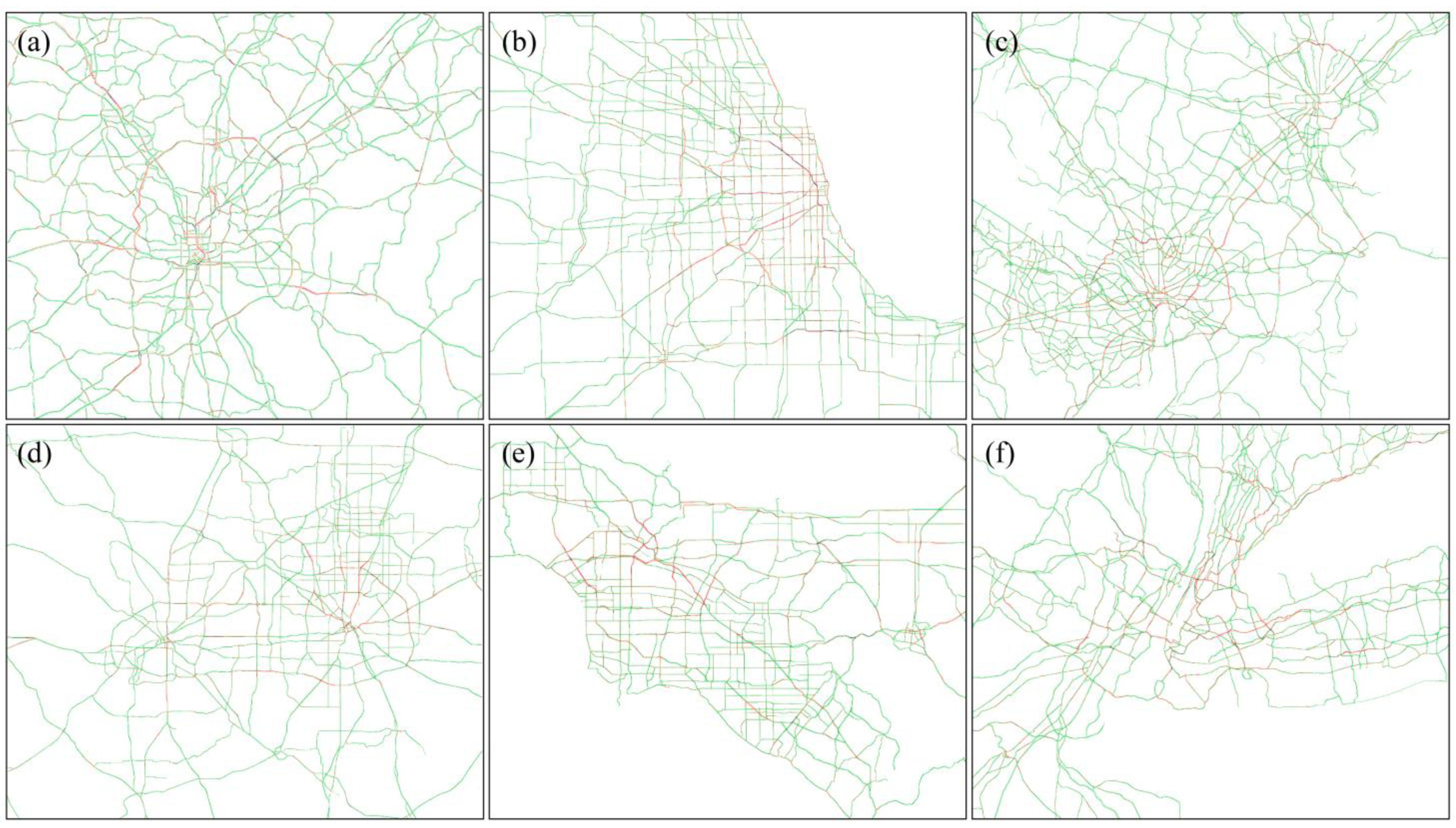
To test the applicability of the metrics for summarizing traffic congestion amount in an area and further making comparisons with other areas, the proposed metrics were applied to six metropolitan areas in the U.S. (Figure 2)—Atlanta (ATL), Chicago (CHI), Dallas and Fort Worth (DFW), Washington, D.C. and Baltimore (DC), Los Angeles (LA), and New York and vicinity (NY). They were chosen considering geographic locations and metropolitan area sizes, and their administrative boundaries were not used to clip the areas. Rather, the rectangular shapes in Figure 2 were used.
The Google Traffic Layer (GTL) API [31] was used to collect traffic information because its applicability for TC research has been demonstrated by multiple researchers recently [32,33,34]. Traffic information from GTL was sampled every 10 min for six months (April through September) in 2022. Samples were not collected on 14 days due to technical issues (05/11, 05/12, 05/13, 05/24, 05/25, 05/26, 06/14, 06/15, 06/16, 06/17, 07/13, 07/14, 08/09, 08/10). Since GTL visualizes congestion severity using green, orange, red, and dark red colors for no traffic delays, medium amount of traffic, traffic delays, and heavy traffic, respectively, the number of color-coded pixels was counted along roads from each image. Road network lengths were calculated from the GTL road images using GIS, and total road pixels were counted along road centers. Then, pixel sizes were calculated from dividing the total road network length by the number of road pixels.
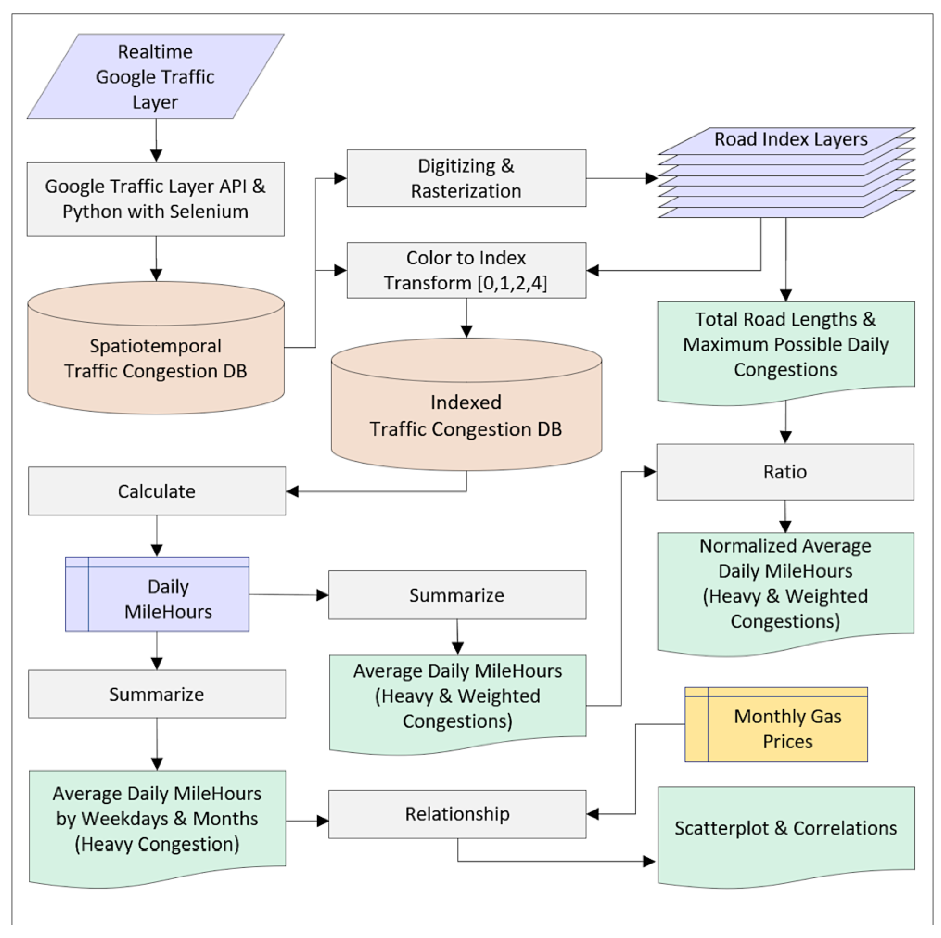
Figure 3 summarizes the overall workflow of data processing and analyses. As indicated in the figure, three TC metrics were calculated by applying Equations (2), (3), and (5). For the non-weighted congestion amounts described in Equation (2), the GTL’s dark-red-coded pixels were used as the indicator of congestion. Particularly, daily congestion amounts () in mileHours were calculated as follows:
where P is pixel size in meters, C is the meter to mile conversion factor (i.e., 0.00062137), and is the average number of congestion pixels from 144 10 min samples a day. The value 24 was multiplied to calculate a daily congestion amount with the mileHours unit.
Daily weighted congestion amounts were also calculated using GTL’s color-coded pixels. The empirical weighting values of 0.25, 0.5, and 1.0 were assigned to orange, red, and dark red colors, respectively, after reviewing the literature about GTL [31,32,33,34]. From 144 10 min samples for each day, average numbers of orange (), red (), and dark red () pixels were calculated. Then, daily weighted congestion amounts () in mileHours were calculated as follows:
From daily congestion amounts, average daily congestion amounts were calculated as long-term congestion indicators. Finally, the average daily congestion amounts were normalized by the maximum possible daily congestion (i.e., 24 h total road length). The normalized values are unitless and indicate the ratio of congestion amount out of maximum possible congestion amount. The ratio values of the six areas were scaled to percent values.
3. Results and Discussion
Table 1 shows the congestion amounts of the six metropolitan areas calculated from daily mileHours. The DC area had the longest road length, followed by CHI, DFW, NY, LA, and ATL. The pixel sizes ranged from 20.14 m (ATL) to 27.24 m (LA) and were different among cities because of different GTL zoom levels and map projection effects. Items E and F in Table 1 will be useful when analyzing congestion amounts of a city or a road section. However, they cannot be used for comparison with other cities because of different road network lengths. As a denominator for normalizing the congestion amounts, the maximum possible daily congestion amount (Item G) was calculated by multiplying the total road length (Item C) and 24 h because the target congestion unit was daily mileHour. The normalized average daily congestion (Item H) shows that the NY area had the highest level of heavy congestion during the study period, followed by the LA area. Interestingly, ATL and CHI show less than half of the heavy congestion of NY and LA. DC and DFW show the lowest heavy congestion. When all congestion levels were considered (Item I), the LA area shows the highest congestion ratio, followed by NY. Three metropolitan areas, ATL, CHI, and DC, show similar congestion ratios. DFW shows the lowest congestion ratio. Items H and I show that the normalized mileHours and their normalized derivatives are effective in comparing multiple cities.
From daily congestion amounts, various other congestion characteristics can also be derived. For example, congestion amounts can be summarized by temporal or geographic units. Table 2 shows a summary of daily heavy congestion amounts by weekdays. In Table 2, inter-city comparison is not meaningful because the numbers are not normalized. All six cities show significant differences among weekdays. Either Thursday or Friday shows the largest congestion in each city, while Monday, Saturday, and Sunday are relatively smaller. When the Sunday congestion is compared with its peak day (ex., 318.93/785.90 × 100 for NY), NY shows 41%, followed by DC (32%), Chicago (26%), Atlanta (22%), LA (18%), and DFW (8%), which implies that Sunday mobility seems to be associated with urban destinations that people may visit during weekends.
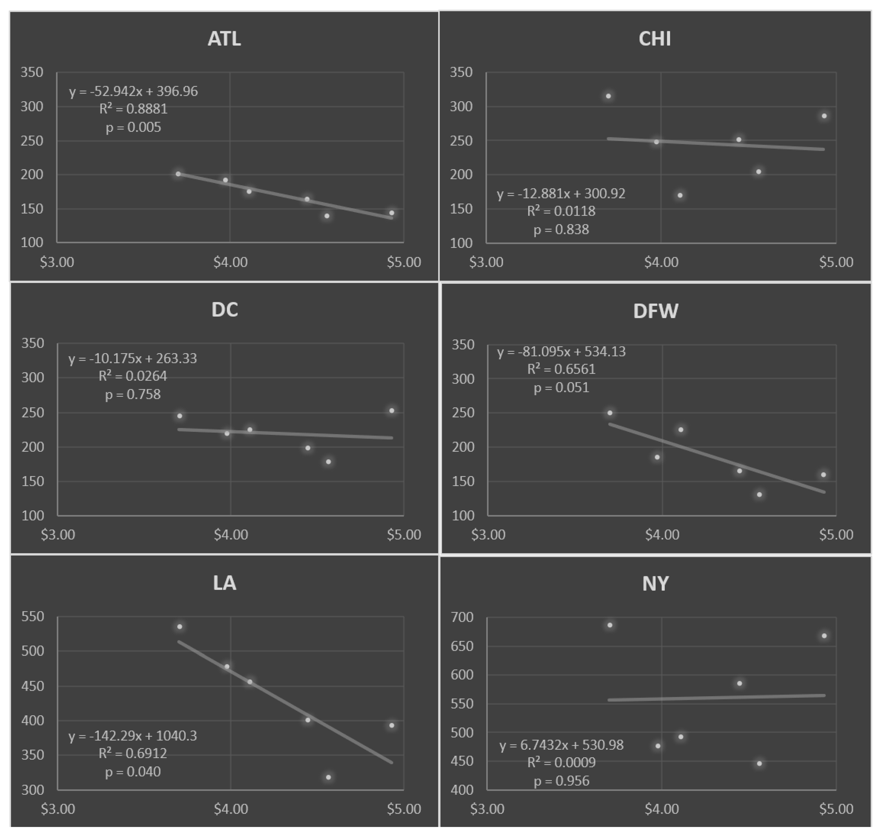
Table 3 shows a summary of heavy congestion amounts by months and is another example of deriving additional information out of daily congestion amounts. Like Table 2, the numbers in Table 3 are not normalized so direct inter-city comparisons are not meaningful; it, however, shows congestion trends over months. Interestingly, July shows the lowest congestion in all cities. The highest congestion appears in September in most cities, except DC in June. When the congestion was analyzed against the U.S. Regular-grade retail gas prices (USD) of (4.109, 4.444, 4.929, 4.559, 3.975, 3.700) per gallon from April to September [35], respectively, correlations were strong in ATL, LA, and DFW, while those with DC, CHI, and NY were very weak, as shown in Figure 4. Considering that DC, CHI, and NY have dense urban areas and public transit systems, it appears that congestion amounts are also affected by the availability of public transportation systems.
Once the average daily congestion amount is calculated, it can be used for calculating the annual average daily congestion (AADC), as the annual average daily traffic (AADT) amount is calculated from daily traffic amounts. If the case study samples cover an entire year, Items E and F in Table 1 can serve as AADC amounts. Considering the study period of six months, they become semi-annual average daily congestion amounts. Likewise, Items H and I in Table 1 serve as AADC ratios. AADC amounts are intuitive by providing mileHours, and AADC ratios are also easy to understand because they deliver percent congestion.
When the TC rankings of the metropolitan areas in Table 1 were compared to the 2022 INRIX Global Traffic Scorecard rankings [10], INRIX ranks CHI first, followed by NY, LA, DC, ATL, and DFW in order, while Table 1 (Item I) ranks LA first, followed by NY, ATL, CHI, DC, and DFW. The difference in rankings seems to be attributed to multiple factors. First, INRIX measures the hours lost from multiple origin–destination travel time records, different from the distanceTime metrics used in this research. Second, INRIX used 1-year data while this research used 6-month data. Considering that monthly variations are quite significant in Table 3, the 6-month data may not represent the whole year accurately. Third, the different sizes of study areas among metropolitan cities may affect the rankings. When more uncongested rural roads are included in a study area, it is likely that TC amount would decrease. Last, the distanceTime metrics are calculated from entire roads, while the INRIX Hours Lost is calculated from samples. In this context, it is difficult to compare INRIX rankings with Table 1 rankings side by side.
Another aspect that needs attention is the interpretation of the distanceTime unit. Because the unit is the product of distance and time, it does not mean exclusively one or the other. For example, suppose an imaginary area’s daily heavy congestion is 240 mileHours. It could mean 240 miles of congestion for an hour, 10 miles of congestion for 24 h, or anything in between. If the area’s afternoon rush hour (ex. 3:00 p.m.–7:00 p.m.) congestion amount is 50% of the average daily congestion amount, then 120 mileHours congestion is expected for four hours, which means 30 miles of congestion, on average, each hour during the afternoon rush hour. In this way, congested road lengths may be estimated from an average daily congestion amount and a temporal congestion pattern.
In this research, samples were collected every 10 min considering that traffic congestion would last at least 10 min, particularly in traffic-heavy metropolitan areas. It, however, is common that traffic congestion lasts much longer. It appears to be necessary to test the effectiveness of different sampling time intervals. In addition, along with the increasing availability of FCD big data, it is necessary to research about using raw FCD data instead of using categorized traffic congestion maps. Specifically, considering that a limitation of this research is the reliance on the color-coded traffic congestion levels of which calculation methods are not published, the FCD data may be a better alternative for more accurate traffic congestion measurements. In this context, research is needed to refine the weighting methods that were described in Section 2.3.
Overall, the case study with six metropolitan areas demonstrates that the congestion amount in distanceTime, calculated from a space-time cube, is very effective in summarizing and analyzing congestion characteristics. It also satisfies multiple attributes for a congestion measure suggested by researchers, including Lomax et al. [2] and Aftabuzzaman [36], because it demonstrates clarity and simplicity, describes the magnitude of congestion, allows for comparison across metropolitan areas, and provides a continuous range of values.
The new metrics presented in this paper may contribute to broad fields where transportation matters. For example, transportation planners in metropolitan planning organizations (MPOs) may quantify traffic congestion amounts by traffic analysis zones (TAZs), cities, or counties for transportation planning. Transportation engineers may also use the metrics to simulate traffic congestion with different road design scenarios. Geographers may use the metrics to study accessibilities, place characteristics, and geographic effects of congestion. Furthermore, the metrics may help estimate various resources wasted by traffic congestion.
4. Conclusions
Measuring traffic congestion amounts that are dynamic and voluminous has been challenging to transport researchers and practitioners. Numerous methods have been developed, but no approaches have been attempted to combine the three components of traffic congestion—intensity, extent, and duration. Considering that traffic congestion is a physical phenomenon that has geographic and temporal dimensions, this research proposed a method to combine them using the space-time framework, researched from a geographic perspective. Multiple metrics were developed to represent the amount of traffic congestion that occurs along one-dimensional linear road features. Particularly, distanceTime unit, average congestion amount, weighted congestion amount, and normalized congestion amount were developed. These metrics were then applied to six metropolitan areas to demonstrate their applicability in real-world scenarios. Google Traffic Layer datasets were used for the case study, and the amounts of heavy congestion, weighted congestion, and normalized congestion were calculated. Results showed that the metrics were effective in summarizing congestion amounts, particularly using the average daily congestion amounts in the mileHours unit. When comparing six metropolitan areas using the normalized average daily heavy congestion amounts, New York and its vicinity showed the largest congestion, but Los Angeles and its vicinity showed the largest congestion when all congestion levels were included in the average daily weighted congestion amounts. The proposed metrics were also useful for further investigation of weekday traffic patterns, monthly traffic patterns, as well as the relationship between traffic amounts and other factors such as gas prices. Furthermore, the new metrics may be used for estimating the total distance of congested roads using past congestion amount information if the hourly congestion pattern is known. Like AADT, the new metrics, including, but not limited to, annual average daily congestion amounts, may help transportation planners, researchers, and practitioners by providing an effective toolset for summarizing congestion amounts intuitively and effectively.
Author Contributions
Conceptualization, Jeong Seong and Hyunmin Kim; methodology, Jeong Seong, Hyunmin Kim, Yunsik Kim, Hyewon Goh and Ana Stanescu; formal analysis, Jeong Seong, Yunsik Kim and Ana Stanescu; investigation, Jeong Seong, Hyewon Goh and Yunsik Kim; resources, Jeong Seong and Ana Stanescu; data curation, Hyunmin Kim, Yunsik Kim and Hyewon Goh; writing—original draft preparation, Jeong Seong; writing—review and editing, Ana Stanescu, Yunsik Kim and Hyewon Goh; visualization, Jeong Seong; project administration, Jeong Seong; funding acquisition, Jeong Seong and Yunsik Kim. All authors have read and agreed to the published version of the manuscript.
Funding
This research was supported by MSIT (Ministry of Science, ICT), Korea, under the High-Potential Individuals Global Training Program (RS-2022-00155411) supervised by the IITP (Institute for Information & Communications Technology Planning & Evaluation).
Data Availability Statement
A sample dataset is available upon request to the corresponding author.
Acknowledgments
Authors thank Byungyun Yang and Jeongu Lee at Dongguk University, Yena Song at Chonnam National University, and Chul Sue Hwang and Hyeokjin Hong at Kyung Hee University for administrative and technical support.
Conflicts of Interest
The authors declare no conflict of interest. The funder had no role in the design of the study; in the collection, analyses, or interpretation of data; in the writing of the manuscript; or in the decision to publish the results.
References
- Falcocchio, J.C.; Levinson, H.S. Road Traffic Congestion: A Concise Guide; Springer: New York, NY, USA, 2015. [Google Scholar] [CrossRef]
- Lomax, T.; Turner, S.; Shunk, G. NCHRP Report 398: Quantifying Congestion: Volume 1—Final Report; Transportation Research Board, National Research Council: Washington, DC, USA, 1997; Available online: http://onlinepubs.trb.org/onlinepubs/nchrp/nchrp_rpt_398.pdf (accessed on 6 January 2023).
- Afrin, T.; Yodo, N. A Survey of road traffic congestion measures towards a sustainable and resilient transportation system. Sustainability 2020, 12, 4660. [Google Scholar] [CrossRef]
- Rahman, M.M.; Najaf, P.; Fields, M.G.; Thill, J.C. Traffic congestion and its urban scale factors: Empirical evidence from American urban area. Int. J. Sustain. Transp. 2022, 16, 406–421. [Google Scholar] [CrossRef]
- Rao, A.M.; Rao, K.R. Measuring urban traffic congestion—A review. Int. J. Traffic Transp. Eng. 2012, 2, 286–305. [Google Scholar] [CrossRef] [Green Version]
- Schrank, D.; Lomax, T. The 2005 Annual Urban Mobility Report; Texas Transportation Institute: Bryan, TX, USA, 2005. [Google Scholar]
- Kumapley, R.K.; Fricker, J.D. Review of methods for estimating vehicle miles traveled. Transp. Res. Rec. 1996, 1551, 59–66. [Google Scholar] [CrossRef]
- Maitra, B.; Sikdar, P.K.; Dhingra, S.L. Modeling congestion on urban roads and assessing level of service. J. Transp. Eng. 1999, 125, 508–514. [Google Scholar] [CrossRef]
- Gajjar, R.; Mohandas, D. Critical assessment of road capacities on urban roads—A Mumbai case-study. Transp. Res. Proc. 2016, 17, 685–692. [Google Scholar] [CrossRef]
- Pishue, B. 2022 Global Traffic Scorecard; INRIX: Kirkland, WA, USA, 2023. [Google Scholar]
- Hägerstrand, T. What about people in regional science? Pap. Reg. Sci. Assoc. 1970, 24, 6–21. [Google Scholar] [CrossRef]
- Kraak, M.-J. The space-time cube revisited from a geovisualization perspective. In Proceedings of the 21st International Cartographic Conference 2003, Durban, South Africa, 10–16 August 2003. [Google Scholar]
- Kwan, M.-P. Space-time and integral measures of individual accessibility: A comparative analysis using a point-based framework. Geogr. Anal. 1998, 30, 191–216. [Google Scholar] [CrossRef]
- Miller, H.J. Time Geography and Space–Time Prism. In International Encyclopedia of Geography: People, the Earth, Environment and Technology; Richardson, D., Castree, N., Goodchild, M.F., Kobayashi, A., Liu, W., Marston, R.A., Eds.; Wiley: Hoboken, NJ, USA, 2017; pp. 1–19. [Google Scholar] [CrossRef]
- Siabato, W.; Claramunt, C.; Ilarri, S.; Manso-Callejo, M.A. A Survey of modelling trends in temporal GIS. ACM Comput. Surv. 2018, 51, 1–41. [Google Scholar] [CrossRef] [Green Version]
- Couclelis, H. Space, time, geography. Geogr. Inf. Syst. 1999, 1, 29–38. [Google Scholar]
- Shellito, B.A. Introduction to Geospatial Technologies, 5th ed.; W. H. Freeman: New York, NY, USA, 2019. [Google Scholar]
- Egenhofer, M.J.; Frank, A.U. Object-oriented modeling for GIS. J. Urban Reg. Inf. Syst. Assoc. 1992, 4, 3–19. [Google Scholar]
- McIntosh, J.; Yuan, M. A framework to enhance semantic flexibility for analysis of distributed phenomena. Int. J. Geogr. Inf. Sci. 2005, 19, 999–1018. [Google Scholar] [CrossRef]
- Worboys, M. A model for spatio-temporal information. In Proceedings of the 5th International Symposium on Spatial Data Handling, Charleston, SC, USA, 3–7 August 1992. [Google Scholar]
- Llaves, A.; Kuhn, W. An event abstraction layer for the integration of geosensor data. Int. J. Geogr. Inf. Sci. 2014, 28, 1085–1106. [Google Scholar] [CrossRef] [Green Version]
- Peuquet, D.J.; Duan, N. An event-based spatiotemporal data model (ESTDM) for temporal analysis of geographical data. Int. J. Geogr. Inf. Syst. 1995, 9, 7–24. [Google Scholar] [CrossRef]
- Yuan, M. Representing complex geographic phenomena in GIS. Cartogr. Geogr. Inf. Sci. 2001, 28, 83–96. [Google Scholar] [CrossRef]
- Choi, J.; Seong, J.C.; Kim, B.; Usery, E.L. Innovations in individual feature history management—The significance of feature-based temporal model. GeoInformatica 2008, 12, 1–20. [Google Scholar] [CrossRef]
- Usery, E.L. A feature-based geographic information system model. Photogramm. Eng. Remote Sens. 1996, 62, 833–838. [Google Scholar]
- Usery, E.L.; Timson, G.; Coletti, M. A Multidimensional Representation Model of Geographic Features: U.S. Geological Survey Open-File Report 2015-1241; U.S. Geological Survey: Reston, VA, USA, 2015. [Google Scholar] [CrossRef] [Green Version]
- Gimblett, H.R. Integrating Geographic Information Systems and Agent-Based Modeling Techniques for Simulating Social and Ecological Processes; Oxford University Press: New York, NY, USA, 2002. [Google Scholar]
- Torrens, P.M. High-resolution space–time processes for agents at the built–human interface of urban earthquakes. Int. J. Geogr. Inf. Sci. 2014, 28, 964–986. [Google Scholar] [CrossRef]
- Yu, C.; Peuquet, D.J. A GeoAgent-based framework for knowledge-oriented representation: Embracing social rules in GIS. Int. J. Geogr. Inf. Sci. 2009, 23, 923–960. [Google Scholar] [CrossRef]
- Bruwer, M.M.; Andersen, S.J. Exploiting COVID-19 related traffic changes to evaluate flow dependency of an FCD-defined congestion measure. Env. Plan. B-Urban Anal. City Sci. 2022, 23998083221081529. [Google Scholar] [CrossRef]
- Google. Use Layers to Find Places, Traffic, Terrain, Biking & Transit. Available online: https://support.google.com/maps/answer/3092439 (accessed on 31 December 2022).
- Bian, C.; Yuan, C.; Kuang, W.; Wu, D. Evaluation, classification, and influential factors analysis of traffic congestion in Chinese cities using the online map data. Math. Probl. Eng. 2016, 2016, 1693729. [Google Scholar] [CrossRef] [Green Version]
- García-Ramírez, Y. Developing a traffic congestion model based on google traffic data: A case study in Ecuador. In Proceedings of the 6th International Conference on Vehicle Technology and Intelligent Transport Systems, Virtual, 2–4 May 2020. [Google Scholar] [CrossRef]
- Ji, S.H.; Seong, J.C.; Stanescu, A.; Hwang, C.S.; Lee, Y. Spatiotemporal traffic database construction with Google real-time traffic information and spatiotemporal congestion pattern analysis: A case study of Montgomery County, Maryland, USA. J. Korean Geogr. Soc. 2021, 56, 265–276. [Google Scholar] [CrossRef]
- EIA (U.S. Energy Information Administration). U.S. Regular All Formulations Retail Gasoline Prices (Dollars per Gallon). Available online: https://tinyurl.com/bdzx4mjs (accessed on 4 January 2023).
- Aftabuzzaman, M. Measuring traffic congestion: A critical review. In Proceedings of the 30th Australasian Transport Research Forum, Melbourne, Australia, 25–27 September 2007. [Google Scholar]
Figure 1.
A space-time cube with traffic congestion intensity levels in different colors—green for free flow, orange for light congestion, red for medium congestion, and dark red for heavy congestion.
Figure 1.
A space-time cube with traffic congestion intensity levels in different colors—green for free flow, orange for light congestion, red for medium congestion, and dark red for heavy congestion.

Figure 2.
Case study areas and sample snapshot images. The images show the extent of six study areas and their traffic intensity levels identified with the Google Traffic Layer API at 5:00 p.m. (local time) on Friday, 22 April 2022. The map scales are not the same. (a) Atlanta, GA, USA; (b) Chicago, IL, USA; (c) Washington, DC, USA and Baltimore, MD, USA; (d) Dallas and Fort Worth, TX, USA; (e) Los Angeles, CA, USA; (f) New York, NY, USA.

Figure 3.
Workflow of data processing and analyses.

Figure 4.
Monthly average gas prices in USD (x-axis) vs. monthly average daily heavy traffic congestion amounts in mileHours (y-axis).
Figure 4.
Monthly average gas prices in USD (x-axis) vs. monthly average daily heavy traffic congestion amounts in mileHours (y-axis).


Table 1.
Traffic congestion metrics of six U.S. metropolitan areas.
| Metrics | ATL | CHI | DC | DFW | LA | NY |
|---|---|---|---|---|---|---|
| A. Number of road pixels | 250,481 | 319,232 | 375,210 | 267,291 | 219,642 | 278,153 |
| B. Total road length (meters) | 5,044,678 | 8,041,366 | 8,926,347 | 7,219,155 | 5,982,216 | 6,408,844 |
| C. Total road length (miles) | 3135 | 4997 | 5547 | 4486 | 3717 | 3982 |
| D. Pixel size (meters) | 20.14 | 25.19 | 23.79 | 27.01 | 27.24 | 23.04 |
| E. Average daily heavy congestion (mileHours) | 171 | 245 | 220 | 188 | 433 | 558 |
| F. Average daily weighted congestion (mileHours) | 1744 | 2720 | 2790 | 1842 | 3516 | 3260 |
| G. Maximum possible daily congestion (mileHours) | 75,231 | 119,920 | 133,118 | 107,658 | 89,212 | 95,574 |
| H. Normalized average daily heavy congestion (%) | 0.23 | 0.20 | 0.17 | 0.17 | 0.48 | 0.58 |
| I. Normalized average daily weighted congestion (%) | 2.32 | 2.27 | 2.10 | 1.71 | 3.94 | 3.41 |
Table 2.
Average daily heavy congestion amounts by weekday (units: mileHours).
| Weekday | ATL | CHI | DC | DFW | LA | NY |
|---|---|---|---|---|---|---|
| Monday | 134.08 | 182.12 | 166.13 | 184.28 | 319.03 | 459.32 |
| Tuesday | 203.31 | 277.88 | 275.26 | 245.02 | 546.92 | 593.38 |
| Wednesday | 229.42 | 285.67 | 293.93 | 256.07 | 592.60 | 669.13 |
| Thursday | 231.20 | 336.53 | 301.31 | 261.19 | 642.73 | 748.90 |
| Friday | 223.45 | 384.15 | 283.55 | 259.33 | 623.05 | 785.90 |
| Saturday | 148.82 | 178.22 | 157.61 | 93.56 | 274.84 | 392.03 |
| Sunday | 51.96 | 100.37 | 96.68 | 51.09 | 112.68 | 318.93 |
Table 3.
Average daily heavy congestion amounts summarized by month (units: mileHours).
| Month | ATL | CHI | DC | DFW | LA | NY |
|---|---|---|---|---|---|---|
| April | 175.96 | 169.80 | 225.29 | 226.16 | 456.04 | 493.68 |
| May | 165.29 | 251.63 | 198.87 | 166.02 | 400.16 | 585.98 |
| June | 144.23 | 285.19 | 251.58 | 159.74 | 393.79 | 668.54 |
| July | 140.63 | 204.73 | 178.03 | 131.20 | 318.48 | 447.64 |
| August | 191.96 | 248.05 | 220.03 | 185.69 | 478.76 | 476.87 |
| September | 202.25 | 314.86 | 224.80 | 250.53 | 535.55 | 686.58 |
Disclaimer/Publisher’s Note: The statements, opinions and data contained in all publications are solely those of the individual author(s) and contributor(s) and not of MDPI and/or the editor(s). MDPI and/or the editor(s) disclaim responsibility for any injury to people or property resulting from any ideas, methods, instructions or products referred to in the content. |
© 2023 by the authors. Licensee MDPI, Basel, Switzerland. This article is an open access article distributed under the terms and conditions of the Creative Commons Attribution (CC BY) license (https://creativecommons.org/licenses/by/4.0/).
Share and Cite
MDPI and ACS Style
Seong, J.; Kim, Y.; Goh, H.; Kim, H.; Stanescu, A. Measuring Traffic Congestion with Novel Metrics: A Case Study of Six U.S. Metropolitan Areas. ISPRS Int. J. Geo-Inf. 2023, 12, 130. https://doi.org/10.3390/ijgi12030130
AMA Style
Seong J, Kim Y, Goh H, Kim H, Stanescu A. Measuring Traffic Congestion with Novel Metrics: A Case Study of Six U.S. Metropolitan Areas. ISPRS International Journal of Geo-Information. 2023; 12(3):130. https://doi.org/10.3390/ijgi12030130
Chicago/Turabian StyleSeong, Jeong, Yunsik Kim, Hyewon Goh, Hyunmin Kim, and Ana Stanescu. 2023. "Measuring Traffic Congestion with Novel Metrics: A Case Study of Six U.S. Metropolitan Areas" ISPRS International Journal of Geo-Information 12, no. 3: 130. https://doi.org/10.3390/ijgi12030130
Note that from the first issue of 2016, this journal uses article numbers instead of page numbers. See further details here.