Leveraging Deep Convolutional Neural Network for Point Symbol Recognition in Scanned Topographic Maps

Abstract

Point symbols on a scanned topographic map (STM) provide crucial geographic information. However, point symbol recognition entails high complexity and uncertainty owing to the stickiness of map elements and singularity of symbol structures. Therefore, extracting point symbols from STMs is challenging. Currently, point symbol recognition is performed primarily through pattern recognition methods that have low accuracy and efficiency. To address this problem, we investigated the potential of a deep learning-based method for point symbol recognition and proposed a deep convolutional neural network (DCNN)-based model for this task. We created point symbol datasets from different sources for training and prediction models. Within this framework, atrous spatial pyramid pooling (ASPP) was adopted to handle the recognition difficulty owing to the differences between point symbols and natural objects. To increase the positioning accuracy, the k-means++ clustering method was used to generate anchor boxes that were more suitable for our point symbol datasets. Additionally, to improve the generalization ability of the model, we designed two data augmentation methods to adapt to symbol recognition. Experiments demonstrated that the deep learning method considerably improved the recognition accuracy and efficiency compared with classical algorithms. The introduction of ASPP in the object detection algorithm resulted in higher mean average precision and intersection over union values, indicating a higher recognition accuracy. It is also demonstrated that data augmentation methods can alleviate the cross-domain problem and improve the rotation robustness. This study contributes to the development of algorithms and the evaluation of geographic elements extracted from STMs.

1. Introduction

Scanned topographic maps (STMs) store and express geographic information that comprises important representations of landforms and features [1,2]. They are widely applied in the domains of resource development, engineering construction, and military defense [3,4]. Therefore, the extraction of geographic elements from STMs has attracted considerable attention [5,6]. In particular, the recognition and positioning of point symbols on STMs provide geographic and positioning information of geographic elements [7,8]. Examples of point symbols on an STM are shown in Figure 1; the following characteristics of point symbols pose significant challenges in their recognition [9]:

(1)

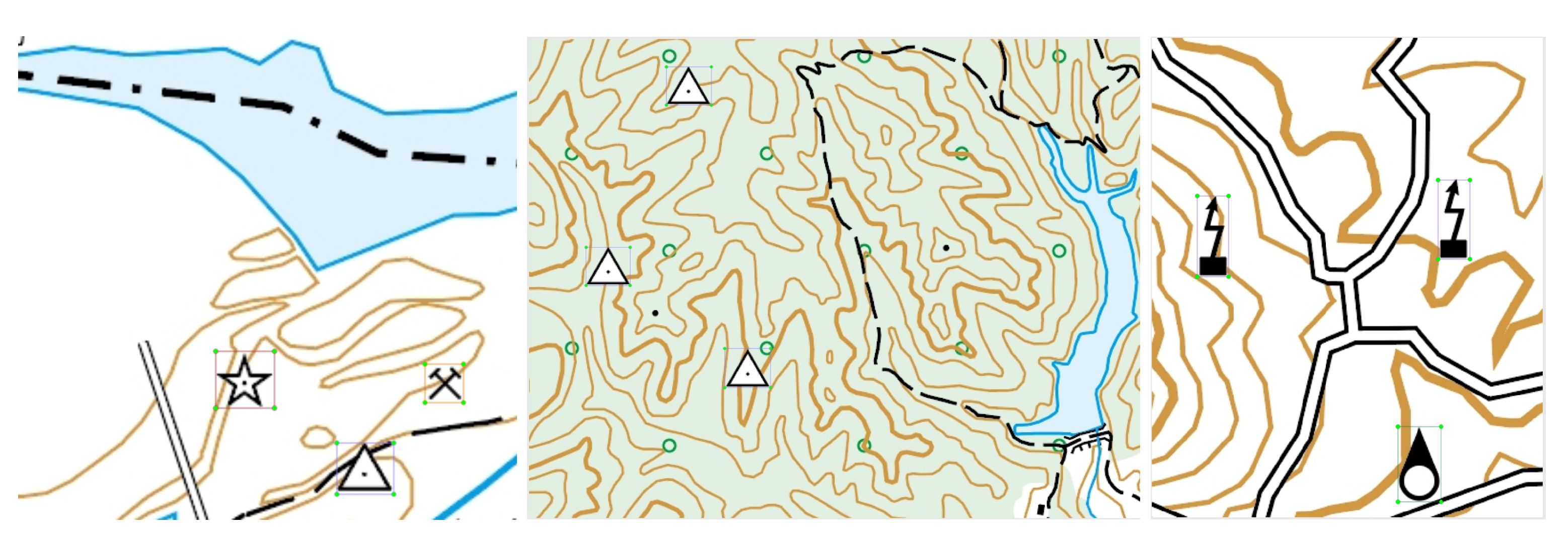
Point symbols are small, have similar shapes, and are generally composed of simple geometric patterns.

(2)

They are difficult to separate from other geographic elements, such as contour lines, using image segmentation [10] or other existing methods.

(3)

Depending on the map quality, the symbols may be blurred, deformed, or discontinuous after scanning.

A review of the literature indicated that several methods have been proposed to overcome these limitations, including template matching, statistical decisions, syntactic structures, and neural networks [11,12,13]. The most primitive methods are based on template matching. Although this method is easy to use, it is susceptible to background noise, resulting in poor recognition performance.

Moreover, improved methods based on template matching approaches have been used to identify point symbols. A fuzzy classification and identification method was proposed in [14] to recognize oil well identifiers in scanned petroleum geological maps. On the basis of the Hough transform algorithm, a method called the shear line segment generalized Hough transform (SLS-GHT), which outperforms other methods in complex scenarios, was proposed in [15] for recognizing point symbols in STMs. However, building the R-table of SLS-GHT is a complicated and time-consuming process with poor generalization ability. Additionally, Reiher et al. [16] recognized symbols using the Hausdorff distance and neural networks. Leyk and Chiang [6] first introduced the concept of geographic context for automated recognition of scanned maps. Pezeshk [17,18,19] has made many contributions to symbol recognition on STMs, mainly using a set of morphological operations. Although these classical methods have yielded results, they still have the following limitations:

(1)

Some STMs cannot be released publicly. Thus, the inadequate sample of point symbols lacks the necessary data support for the study.

(2)

Because symbols frequently overlap with other geographic elements, they are difficult to recognize entirely; thus, it is challenging to achieve both efficient and accurate recognition.

(3)

One centimeter on the topographic map (TM) represents several kilometers of the field. However, the positioning of point symbols in the existing methods is slightly shifted, and the determination of symbol anchors must be improved.

Therefore, we found that advanced models and strategies that are highly efficient, accurate, and robust to noise and other factors are required for point symbol recognition. Recently, with the development of computer vision, various deep convolutional neural networks (DCNNs) have been proposed for solving different image processing tasks, such as object detection [20,21] and semantic segmentation [22,23]. Deep learning has been applied for remote sensing object detection [24,25,26] and identifying dynamic changes in ground objects [27] with high accuracy.

In recent years, convolutional neural networks (CNNs) [28] have been widely used in the field of computer vision, and researchers have applied them to symbol recognition tasks and made significant progress. In [29], a deep transfer learning architecture was proposed for learning a symbol classifier using AlexNet and recognizing multiple point symbols simultaneously to increase the overall efficiency. In [30], a DCNN and graph convolutional network (GCN) were combined to extract and recognize geological map symbols. In [31], deep learning technology was applied to piping and instrumentation diagrams (P&IDs) to recognize symbols and text at an industrially applicable level. In such optical character recognition methods, the foreground and background differ considerably and mostly have a regular shape. However, point symbols on STMs are more abstract and stick to the background, differing in the research questions.

Inspired by the aforementioned studies and considering the characteristics of point symbols, we investigated the potential of object detection methods in point symbol recognition and developed a DCNN model for detecting symbols on STMs. Object detectors can be classified as one-stage or two-stage. Although one-stage detectors sacrifice some accuracy to achieve a high speed, they can achieve similar performance to two-stage detectors or even better performance in recent studies [32]. Therefore, the proposed method is based on one-stage detectors. There are two types of one-stage object detectors: you only look once (YOLO) [33,34,35] and single-shot detector (SSD) [36]. However, STMs differ from other types of images in that the contain a more singular shape of features and require more accurate geographic element recognition, for which traditional object detectors are not well-adapted. Studies [21,37] have indicated that object detectors primarily focus on detecting apparent or large objects and do not perform well in detecting small objects in images. Therefore, dilated convolution, which enlarges the receptive field, has been introduced for detecting small objects in images. Chen et al. [38] inserted a dilated convolution into YOLOv3, and achieved a 5.69% improvement in mean average precision (mAP) compared to the original model for their dataset. Li et al. [39] employed astrous spatial pyramid pooling (ASPP) [40] to extract multiscale features. Wang et al. [41] proposed a simple hybrid dilation convolution framework to alleviate the gridding problem using different dilation rates.

Point symbols and natural objects differ in that the symbols have a single shape and texture feature and stick to other background elements, making it difficult to distinguish between positive and negative samples. Therefore, we employed ASPP instead of spatial pyramid pooling (SPP) [42] in the YOLOv4 network to obtain multiscale information. The new network performed well in point symbol recognition and positioning tasks on STMs. Moreover, we constructed point symbol datasets for the supervised algorithm and proposed two data augmentations to improve the generalization ability of the model. We used the basemap in Cartographic symbols for national fundamental scale maps—Part 1:Specifications for cartographic symbols 1:500, 1:1000 and 1:2000 topographic maps for experiments and symbol recognition. The main contributions of this study can be summarized as follows:

(1)

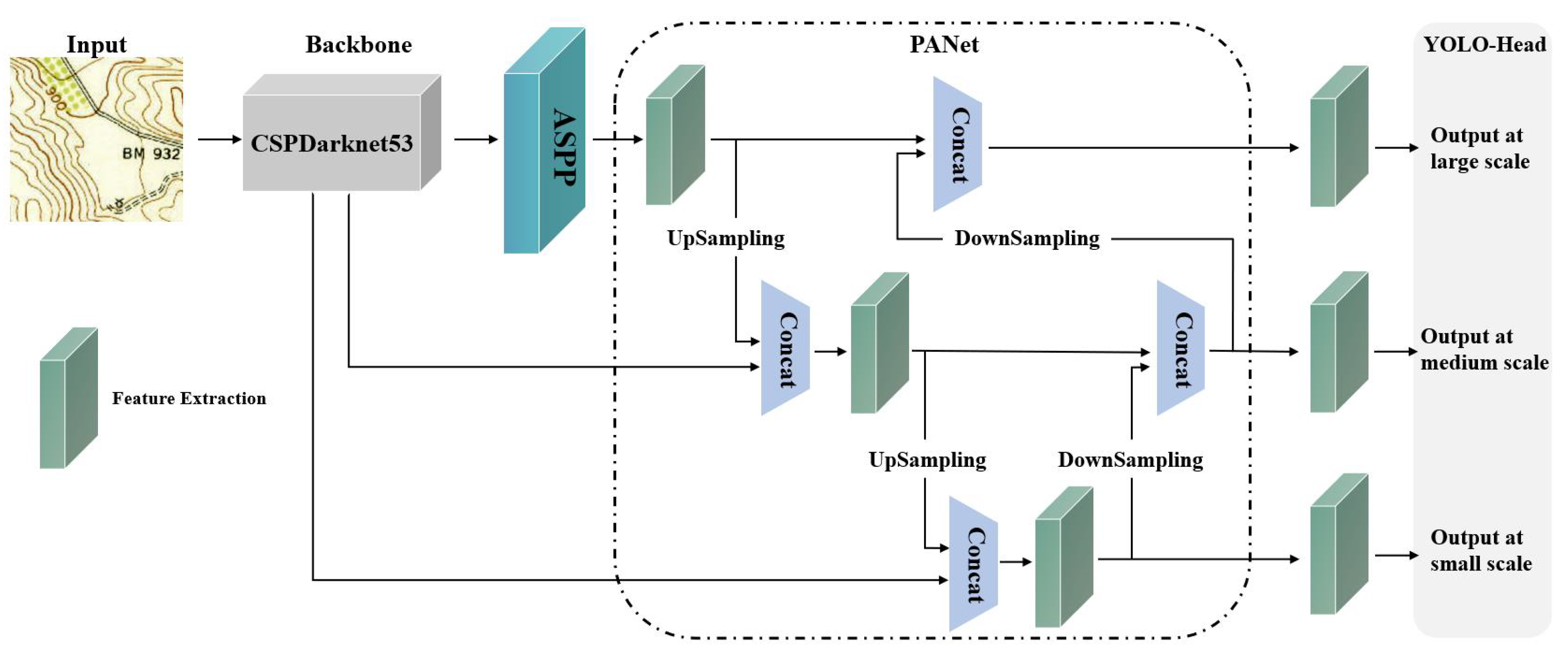
STM point symbol datasets were constructed. Many scanned and vectorized map images were annotated, which comprised 1909 scanned map images and 2505 vectorized map images at different scales. We developed a DCNN model based on YOLOv4 for symbol recognition. The ASPP module, which enlarges the receptive field to obtain more information about the symbol object, was adopted to improve the accuracy and efficiency of symbol recognition.

(2)

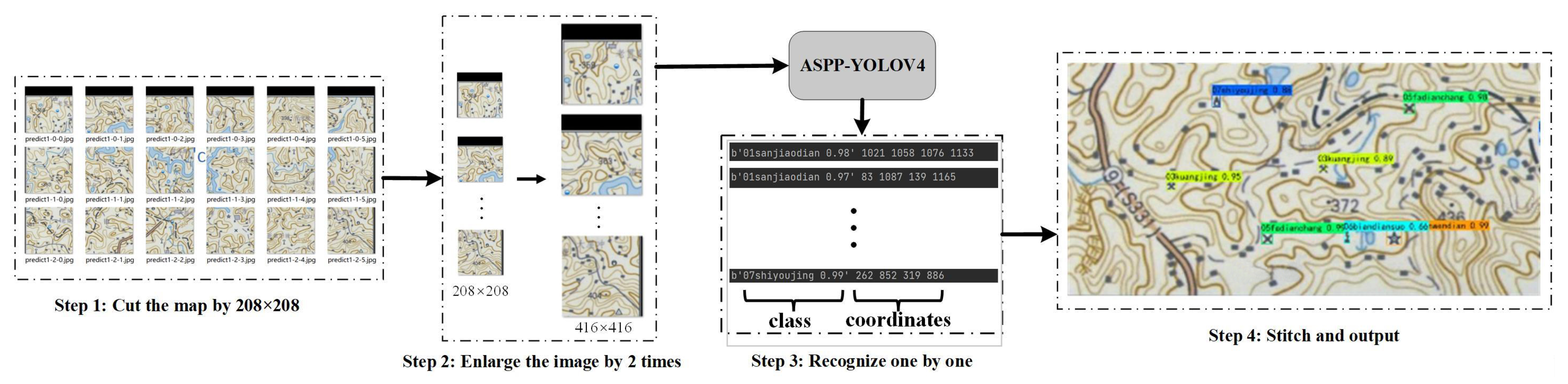
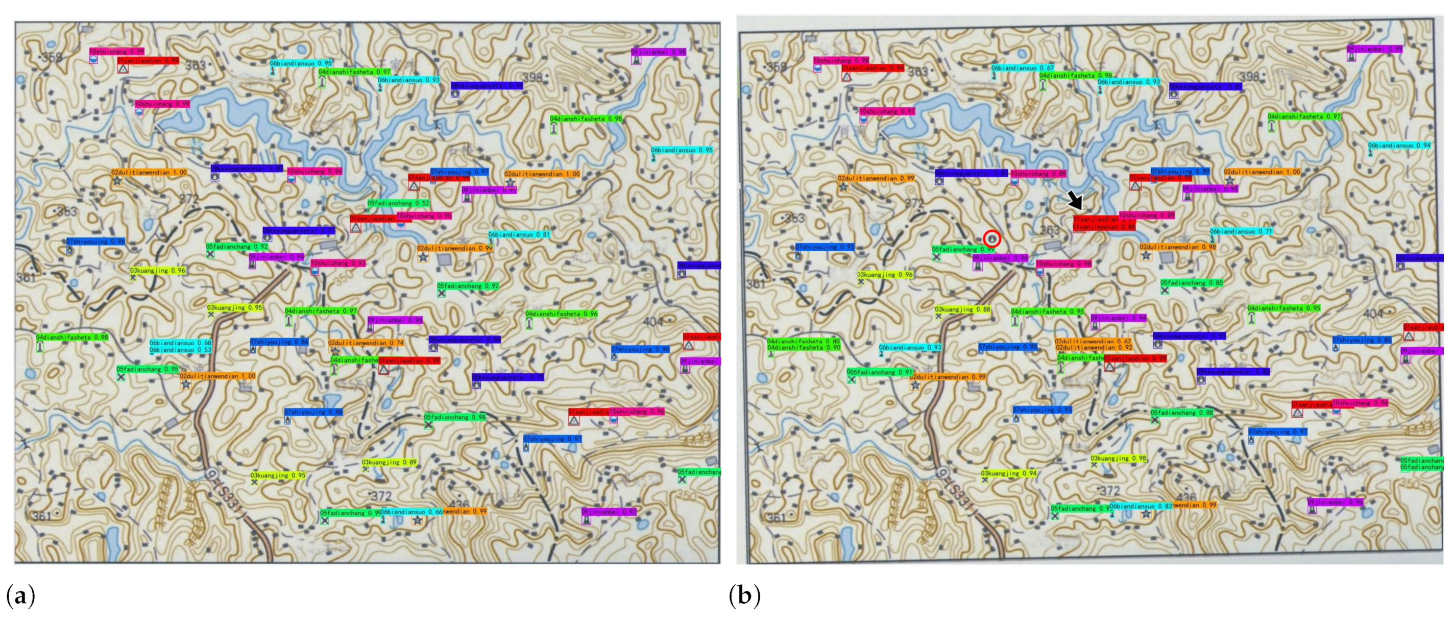
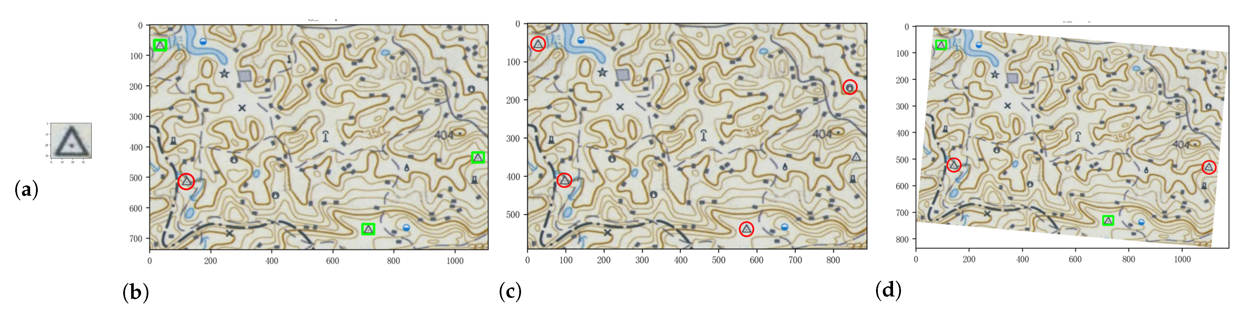
To solve the cross-domain problem caused by datasets comprising maps of different styles and improve the model robustness, two data augmentation methods were designed: Gaussian blur combined with the color jitter method and small-angle rotation with an affine transformation. Additionally, to improve positioning accuracy, the k-means++ clustering method was adopted to generate anchor boxes that were more suitable for our point symbol datasets. A cut-stitch approach was designed for large-scale maps and its effectiveness was tested through several experiments on our dataset.

(3)

We achieved an mAP of 98.11% and a mean intersection over union (mIoU) of 0.876 for point symbol recognition on our test set. The proposed method is the first to employ DCNNs for recognizing point symbols, and it achieved a higher recognition and positioning accuracy than mainstream detectors and classical algorithms.

The remainder of this paper is organized as follows. Section 2 provides a detailed description of the constructed datasets. Section 3 describes the novel variant of YOLOv4, the k-means++ clustering algorithm adopted for point symbol recognition, and the two data augmentation methods used. Section 4 presents the experiments designed to comprehensively compare the proposed model with mainstream detection models and classical algorithms. Finally, Section 5 summarizes the study, highlights its limitations, and provides possible directions for future work.

2. Point Symbol Datasets

A dataset is vital for supervised learning algorithms and provides data support for research on point symbol recognition. Thus, we manually edited the scanned and vectorized map image datasets for the point symbol recognition task. We studied ten types of point symbols as an example, which are presented in

Table 1. The symbols and their identifiers.

The Symbols
The identifiers	I	II	III	IV	V	VI	VII	VIII	IX	X
The meanings	sanjiaodian	dulitianwendian	kuangjing	dianshifasheta	fadianchang	biandiansuo	shiyoujing	kexueguancezhan	jinianbei	shuichang

.

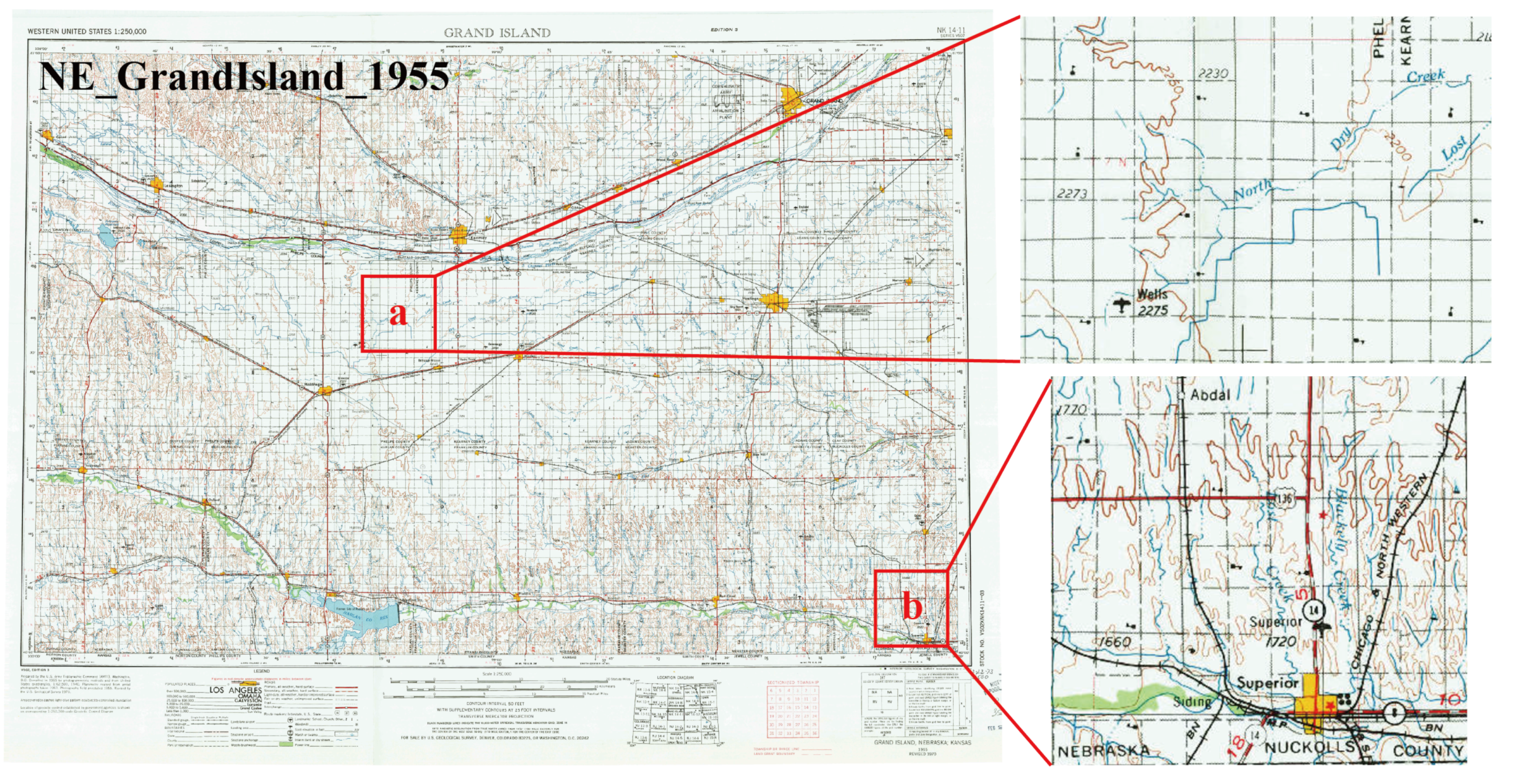
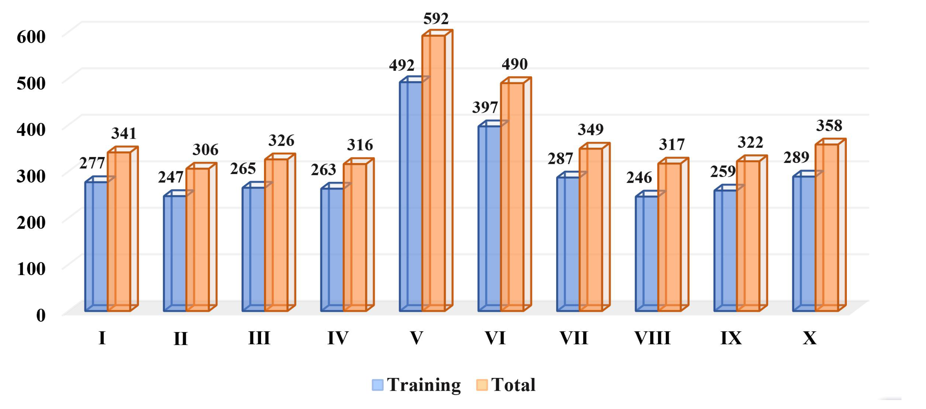
2.1. Scanned Map Dataset for Training and Testing

To train and test our model, we first constructed the scanned map dataset, which comprised 1909 images from a scale of 1:50,000 scanned maps and 3717 single symbols. The dataset was divided into three parts: training, validation, and test sets at a ratio of approximately 8:1:1. Figure 2 shows the statistical results for the training set and total set. There are differences in the numbers of various point symbols, leading to a slight class imbalance but no long-tail distribution. The weighted training method was used to solve this problem such that the model was more focused on a smaller number of symbols. Additionally, this dataset recorded the image categories and coordinates of the point symbols on the STMs. Specific examples are shown in Figure 3.

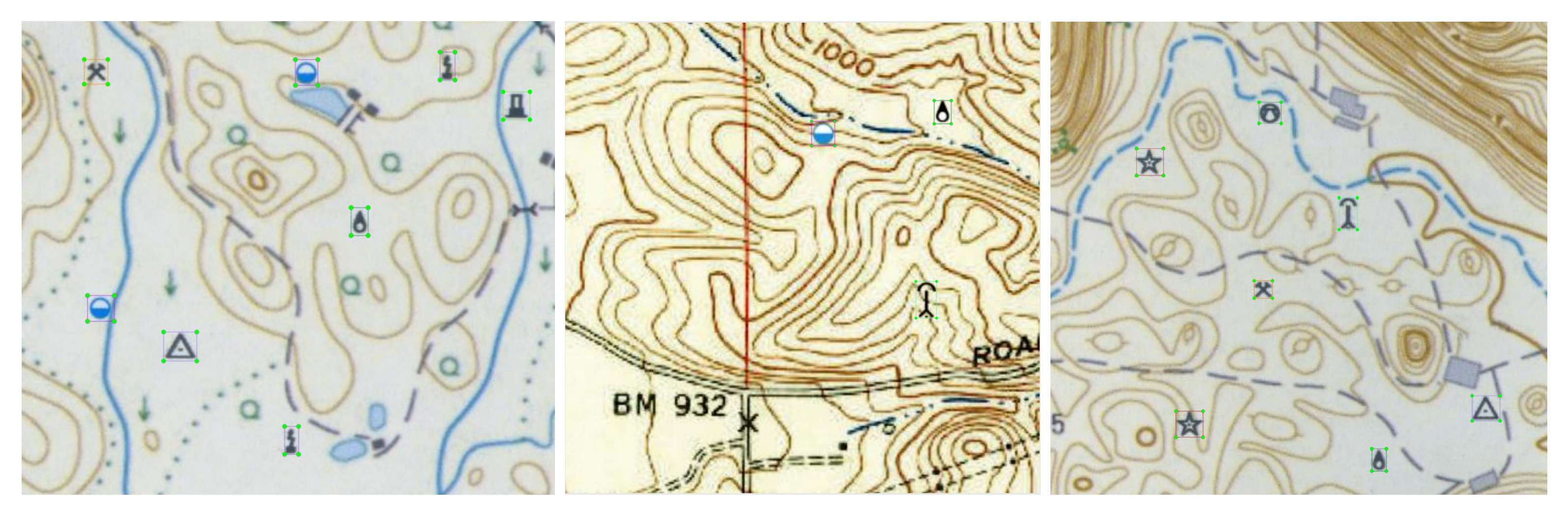
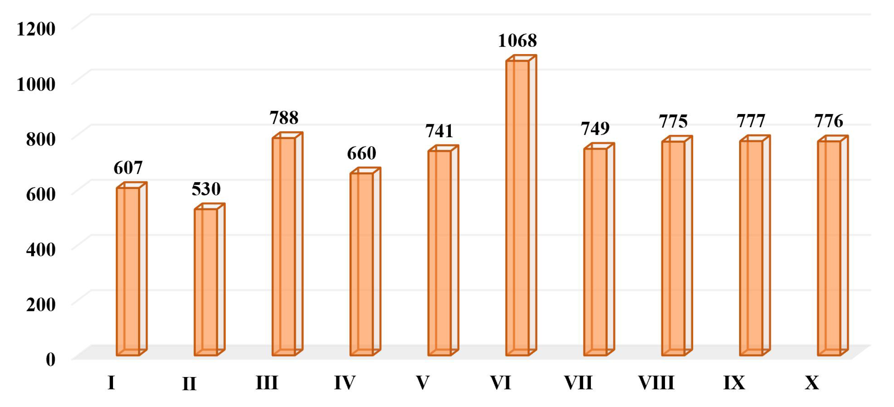
2.2. Vectorized Map Dataset for Training

The other point symbol sub-dataset comprised 2505 images from vectorized maps of different scales. It contained 7471 single symbols, and the numbers of various symbols are shown in Figure 4. The vectorized maps had different textures and clearer symbol images than the scanned maps, as shown in Figure 5. Similar to the scanned map dataset, this vectorized map dataset recorded the image coordinates and symbol categories. To evaluate the generalization ability of the deep learning method for different data sources, this sub-dataset was used as another training set but with varying map styles in the same symbol system. It complemented the symbol dataset of STMs and allowed map diversity.

3. Methods

Both a high detection accuracy and a low computational cost are crucial for practical applications of symbol recognition methods. The YOLOv4 model has been extensively applied in the field of object detection; therefore, we leveraged it to recognize point symbols on STMs. The detection targets in natural images are large and the texture varies widely between different categories, allowing the foreground and background to be easily distinguished, as shown in Figure 6. In contrast, the background of STMs is complex; the point symbols overlap with other geographic elements, and the symbols have similar color and texture information, making it difficult to distinguish between positive and negative samples. Moreover, on STMs, symbols are presented as small densely distributed targets with relatively low-resolution maps, which necessitates targeted improvements to the existing detection framework.

We aimed to comprehensively use dilated convolution in SPP, which uses multiple parallel convolution layers with different dilation rates to extract multiscale features to reduce the loss of feature map details, and proposed ASPP-YOLOv4 to address the problem of small object detection and the insufficient positioning accuracy, as illustrated in Figure 7.

We resized the image to a fixed size to use it as the input for the ASPP-YOLOv4 model. During forward propagation, feature maps of different scales were obtained from the CSPDarknet53 backbone network. Because the point symbols on STMs are small, we adopted the ASPP module and the path aggregation network (PANet) to fuse multiscale feature information to improve the model performance for symbol recognition and positioning tasks. The outputs were three YOLO heads, which were responsible for predicting objects on small, medium, and large scales. The prediction module comprised three parts: object bounding boxes, object categories, and confidence. We used the complete intersection over union (CIoU) loss to avoid the degradation of generalized IoU (GIoU) loss to IoU loss in certain situations. In addition, DIoU_non-maximum suppression (NMS) is employed in our network, which considers the center of the prediction box, resulting in a more accurate recognition of point symbols.

3.1. Dilated Convolution

The space between the standard convolution kernels is injected with voids, which is called a dilated convolution. Dilated convolution uses sparse sampling instead of downsampling, thus enlarging the receptive field without increasing the network depth, number of pooling layers, or number of parameters. The receptive field ($R{F}_n$) is calculated using the following equation:

$$R{F}_n=\left\{\begin{array}{cc}{k}_n,\hfill & n=1\hfill \\ R{F}_{n-1}+(k_n-1)\times S_{n-1},\hfill & n\ge 2\hfill \end{array}\right.$$

(1)

where $k_n$ denotes the size of the convolution kernel and $S_{n-1}$ denotes the stride of the previous layer of the network. Evidently, a larger stride corresponds to a larger receptive field. However, a larger stride size is not always preferable. Dilated convolution is a sparse sampling method, and when multiple dilated convolutions are superimposed, some pixels of the STM image are not used, which results in losses of continuity and relevance of information. Therefore, dilated and standard convolutions are used in parallel in the ASPP-YOLOv4 model.

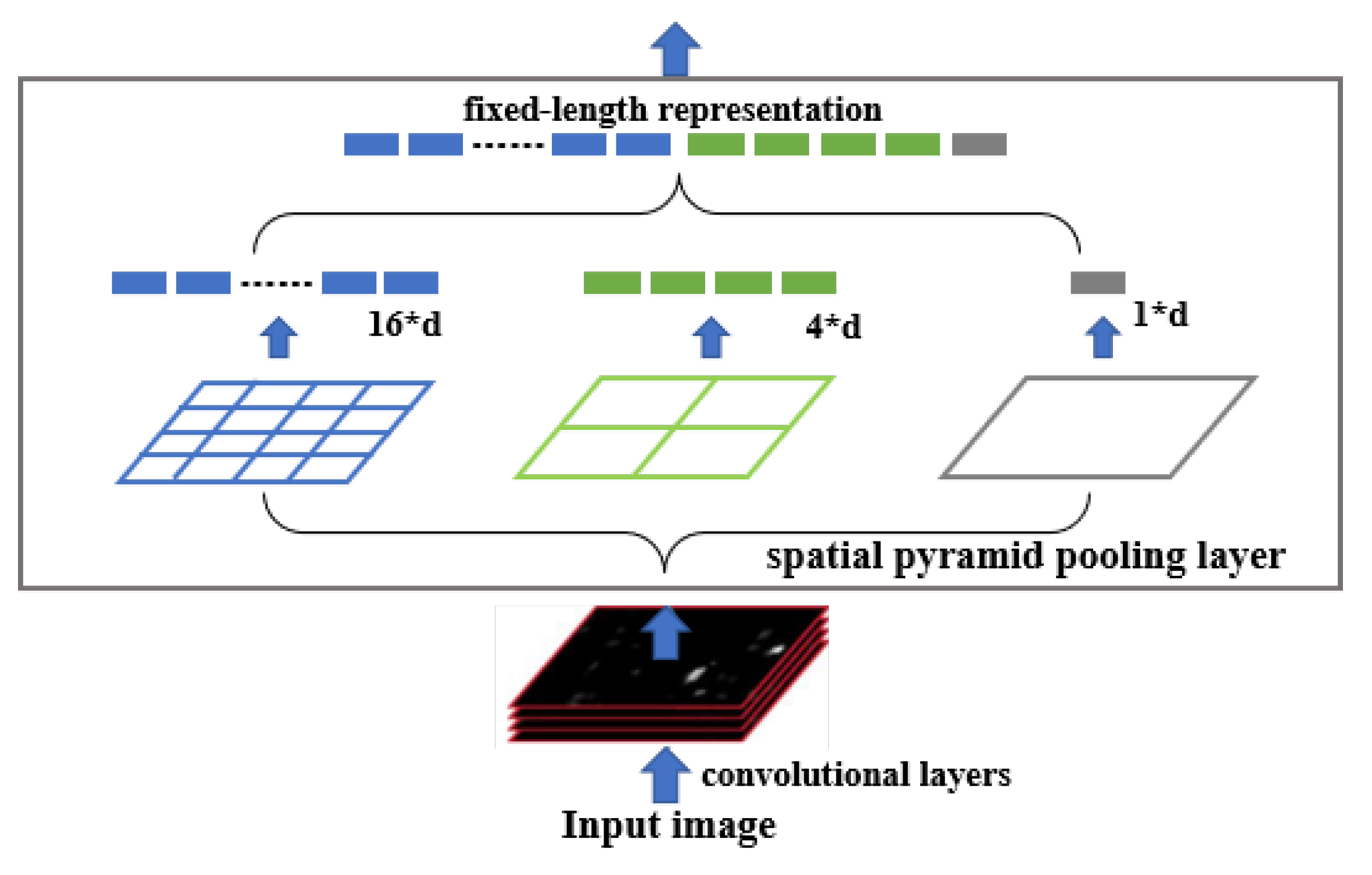
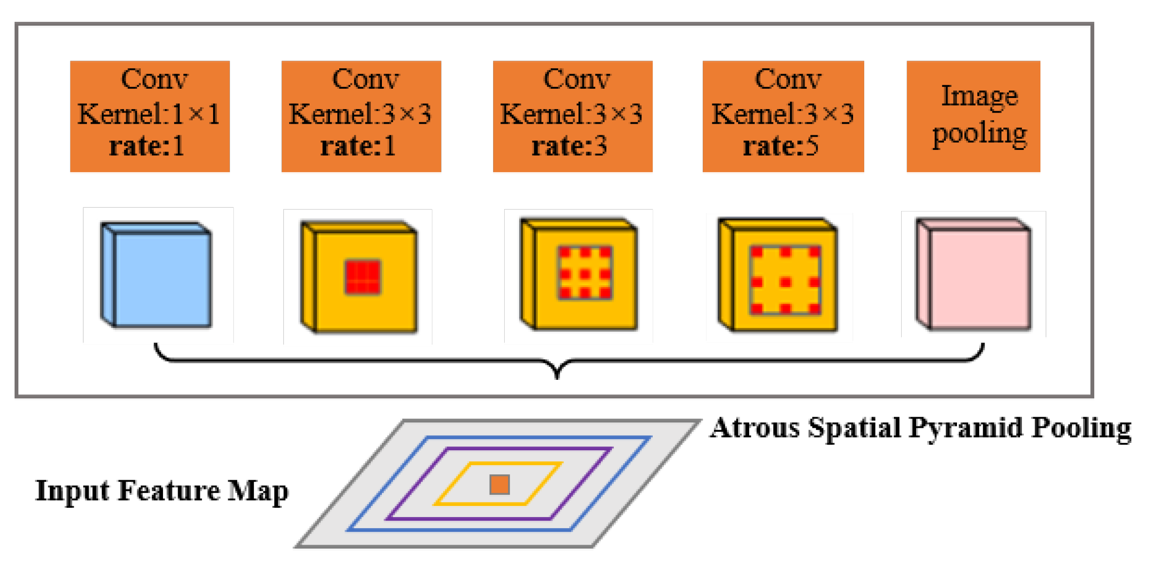
3.2. Atrous Spatial Pyramid Pooling (ASPP)

During a single dilated convolution, the gridding issue causes local information loss, and long-distance information lacks relevance. Inspired by SPP (Figure 8), the ASPP module uses multiscale receptive fields to achieve a balance between global and local features during image processing. The ASPP module uses dilated convolution to replace the maximum pooling in the SPP. As shown in Figure 9, the first branch comprises $1\times 1$ standard convolution, which aims to maintain the original perceptual field; the second to fourth branches comprise depth-separable convolutions with different dilation rates, which aim to perform feature extraction for obtaining different perceptual fields; and the fifth branch comprises the global average pooling of the input to obtain global features. Finally, the feature maps of the five branches are stacked in the channel dimension to fuse information from multiple scales and upsample the desired spatial dimension bilinearly. The ASPP is more accurate and effective for small-object detection tasks involving the extraction of multiscale features.

3.3. Data Augmentation for Generalization Capability

During the training of the ASPP-YOLOv4 model, we applied data augmentation methods to extend the original dataset and improve the generalization and reliability of the model. For training on the scanned and vectorized map datasets, common data augmentation methods were used, such as random cropping, random horizontal and vertical flipping, and random conversion of the original image into a gray image. Furthermore, to enhance the robustness of the proposed symbol recognition model and simulate the distortions that occur during map scanning, such as small angular tilts, an affine transformation data augmentation method [43] was used for the scanned map dataset. Specific examples are presented in Figure 10. The data augmentation method that was only applied to the vectorized map dataset training, the Gaussian blur combined with the color jitter method, as shown in Figure 11. This is because scanned and vectorized maps have different styles, and the model recognition can be improved by transforming the style via image processing.

3.4. Anchor Boxes Based on K-Means++ Clustering

The label bounding boxes of the point symbols in the dataset varied in size. Anchor boxes closer to the symbol label bounding box in size correspond to more accurate detection. However, the anchor frame used by YOLOv4 is within the anchor box range calculated from the natural object dataset, which differs from our dataset. Therefore, we adopted the k-means++ clustering algorithm to obtain the best priors for the anchor boxes in the dataset, which uses the IoU score instead of the Euclidean distance function as an evaluation criterion, as indicated by the following equation:

$$d(box,centroid)=1-IoU(box,centroid)$$

(2)

where $box$ denotes the sample, $centroid$ denotes the center point of the cluster, and $IoU(box,centroid)$ denotes the overlap ratio of the cluster and center boxes.

Using the k-means++ clustering strategy, we experimentally obtained the changes in the average IoU score (avgIoU) corresponding to different numbers of anchors (k-values), as presented in

Table 2. The relationship between the number of anchors and avgIoU is obtained based on the k-means++ clustering algorithm.

k-Values	1	2	3	4	5	6	7	8	9
	62.53	33.43	27.40	25.38	21.43	21.44	19.40	19.41	19.40
		58.64	47.51	33.62	40.40	37.37	37.37	34.34	33.34
			67.72	48.48	33.62	34.63	27.54	27.54	26.54
Anchors				66.71	54.54	48.48	48.48	43.42	43.42
					71.77	59.59	40.72	52.52	37.67
						73.80	59.59	40.72	51.52
							74.79	62.62	62.61
								76.81	53.92
									79.78
avgIoU	0.598	0.698	0.745	0.766	0.799	0.818	0.831	0.843	0.852

. As the number of anchors increased, the avgIoU value continued to increased, but the growth rate decreased in later stages. Considering the complexity of the proposed network, we selected a k value of 9, and obtained the following anchor box values: $\left[\right(19\times 40),(33\times 34),(26\times 54),(43\times 42),(37\times 67),(51\times 52),(62\times 61),(53\times 92),(79\times 78\left)\right]$.

4. Experimental Results and Analysis

In this section, we describe the experiments used to compare the proposed ASPP-YOLOv4 model with mainstream object detectors and state-of-the-art methods with regard to the recognition accuracy, feature visualization, runtime, and generalization capability. We initialized CSPDarknet53 with the pre-trained model parameters from the PASCAL VOC dataset for training ASPP-YOLOv4. All models were implemented using the PyTorch framework on an NVIDIA Quadro P6000 GPU with 24 GB memory. We used the stochastic gradient descent (SGD) optimizer with a momentum of 0.937 to train all the networks. Additionally, the initial learning rate was set to 0.0001 and the step learning strategy was used. In the experiments, we used a frozen training strategy with the same dominance parameters to train over 1000 epochs. The models were trained on the dataset described in Section 2 and tested on the scanned map dataset. Classical algorithms were implemented using Python.

In addition, positioning, classification, and speed evaluations were performed to comprehensively assess the symbol recognition results. The positioning evaluation indicator is the mIoU, which is the area ratio of the intersection of the predicted and true-positive boxes to the result of their union. The precision, recall, F1 score, and mAP were used as performance metrics to evaluate the classification performance of the models. The average precision (AP) for symbol recognition was computed using an IoU threshold of 0.5. The average inference time, which is calculated as the total time spent for the symbol recognition process divided by the number of images detected, was used as a speed evaluation indicator.

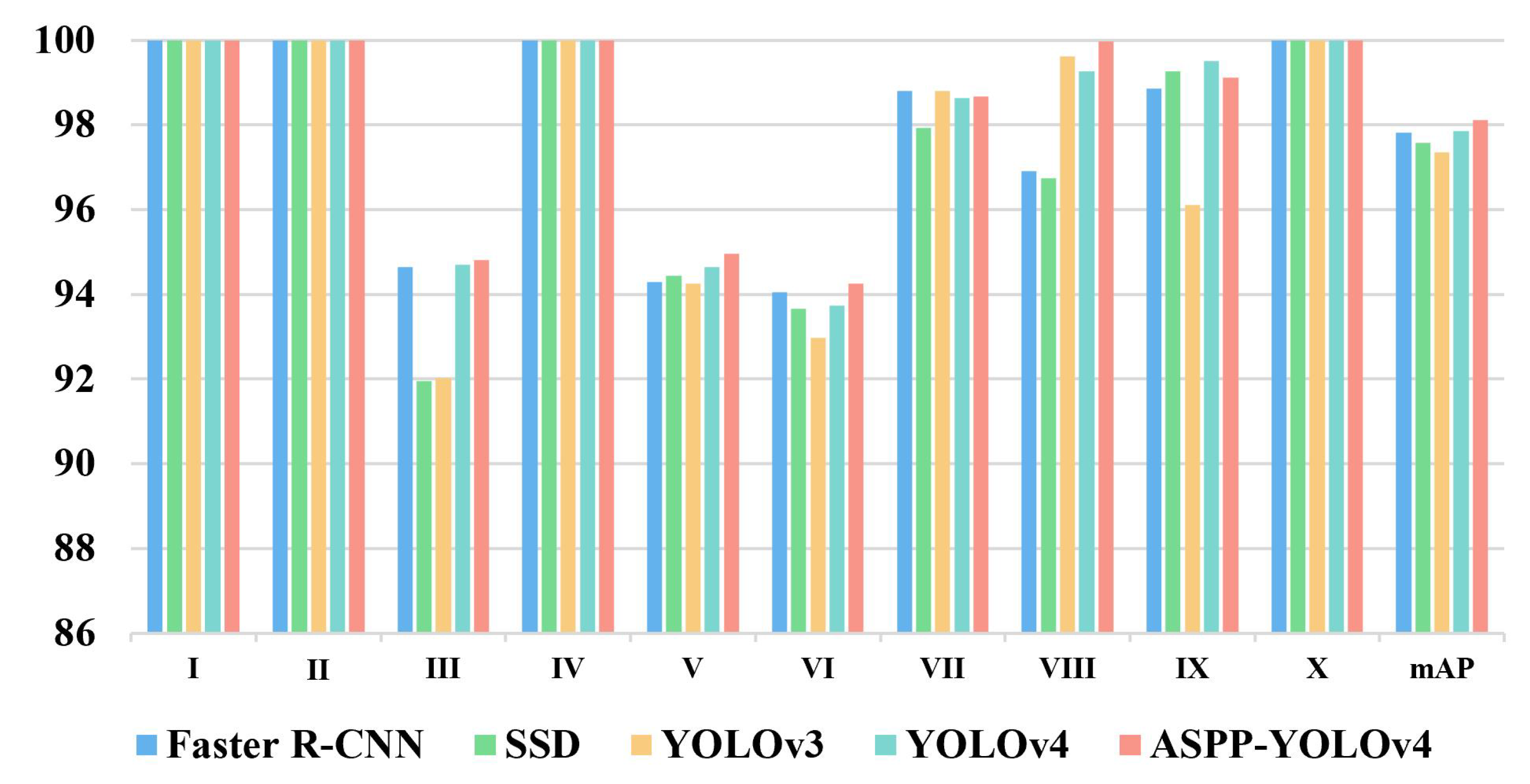
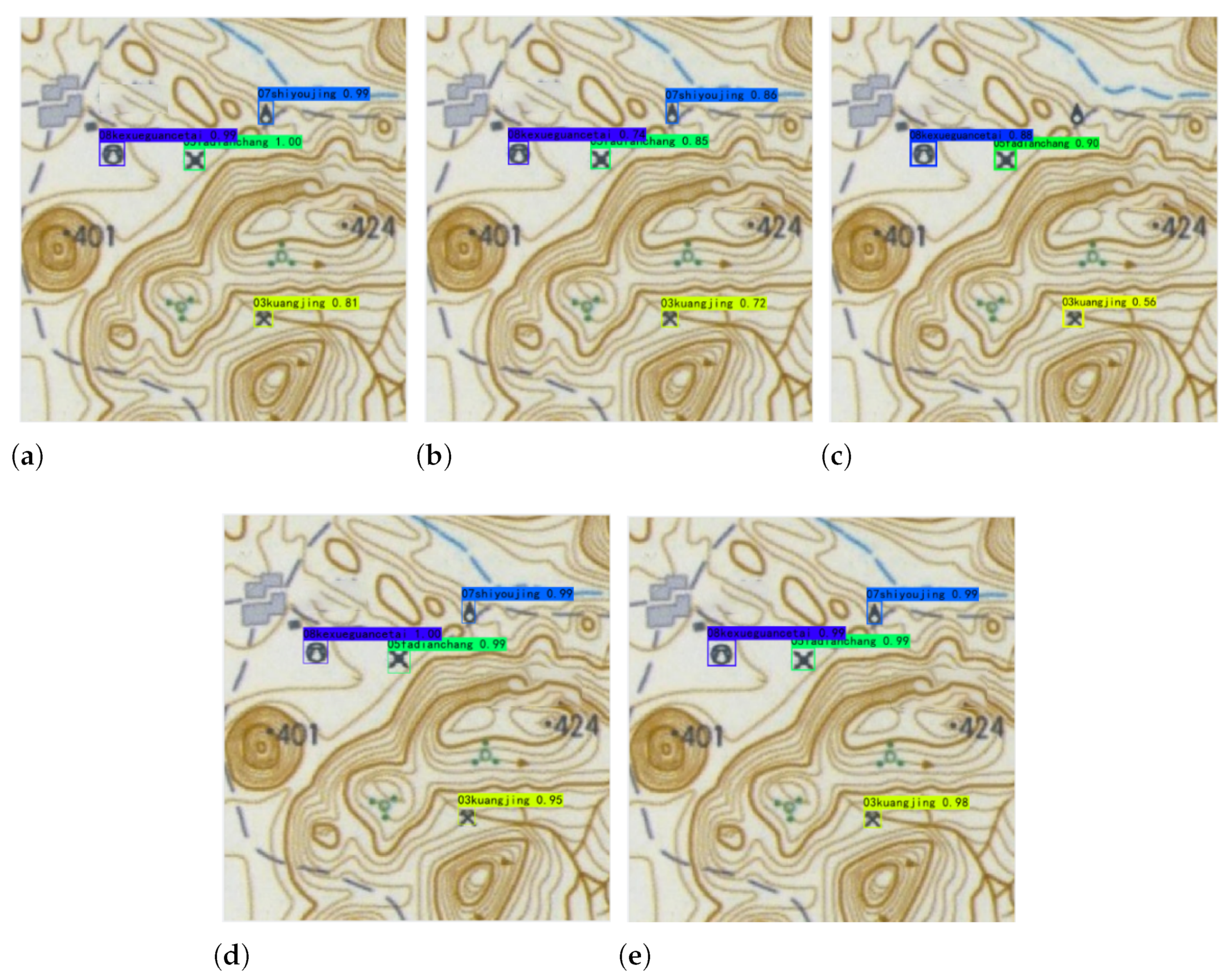
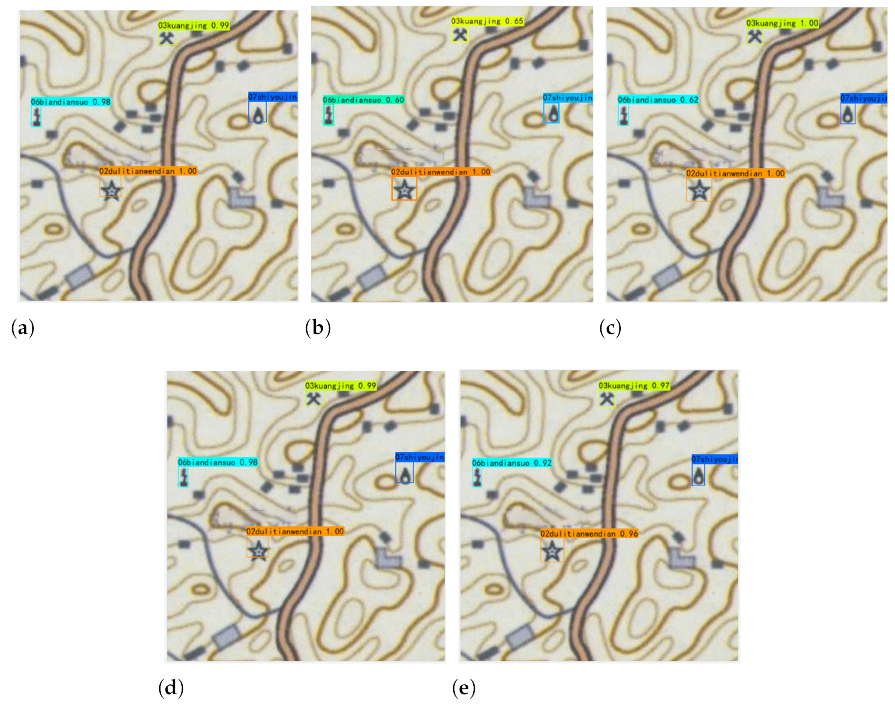
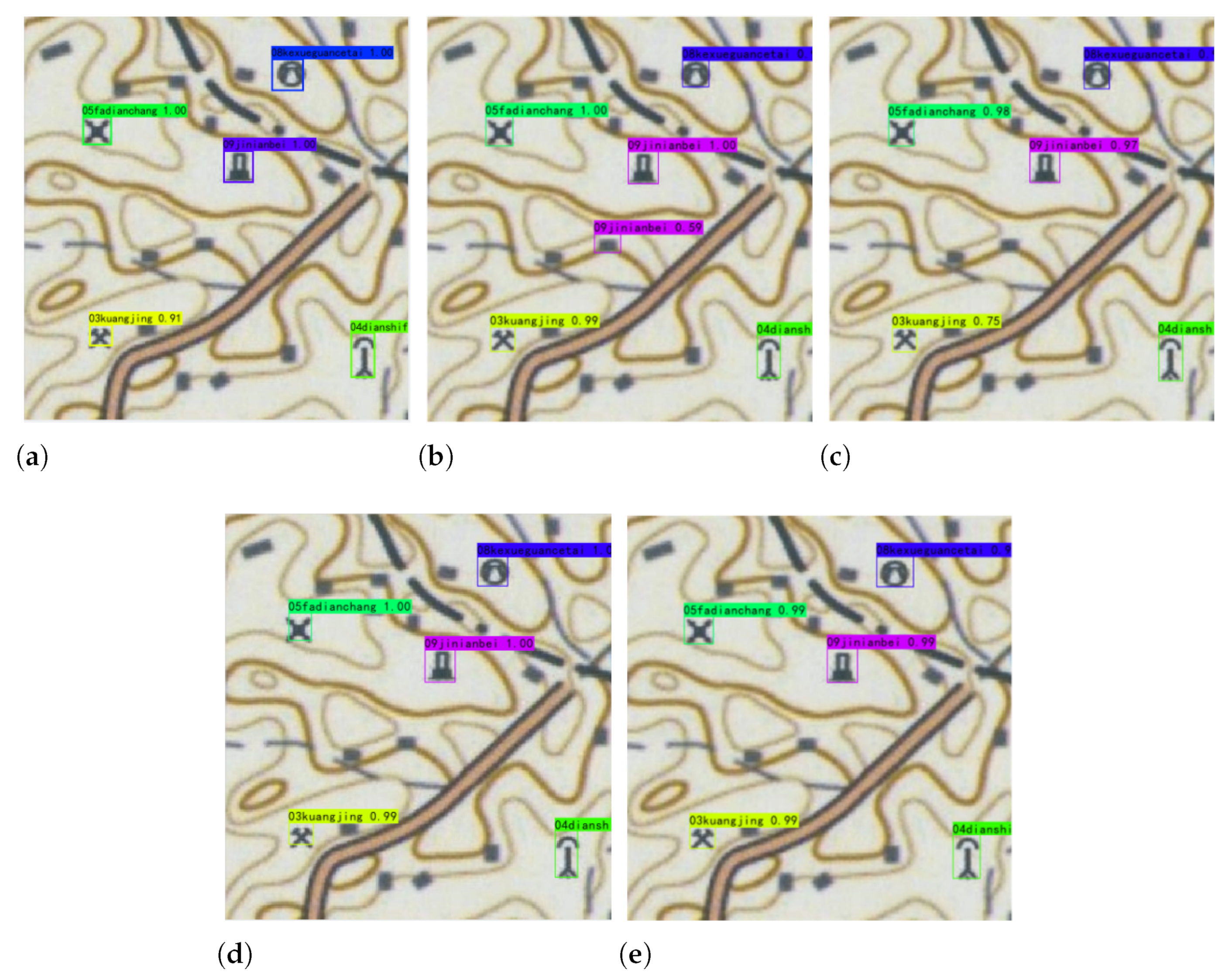
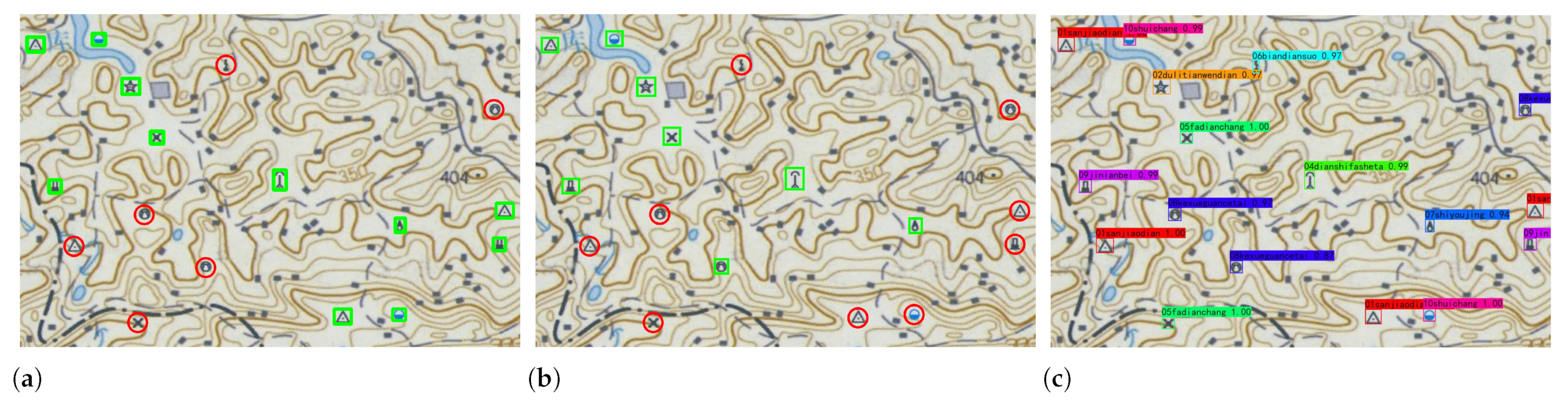
4.1. Comparison of Different Object Detectors Recognition Models

In this section, the performances of four mainstream object detectors, faster R-CNN [38], VGG-SSD [36], YOLOv3 [33], and YOLOv4 [34] are compared with that of the proposed model to validate the proposed method.

Table 3. Experimental results of different models for symbol recognition.

Model	Precision	Recall	F1 Score	mAP	mIoU
Faster R-CNN	97.21	96.44	96.82	97.81	0.874
VGG-SSD	96.68	96.59	96.63	97.58	0.865
YOLOv3	92.89	95.68	94.26	97.35	0.824
YOLOv4	96.38	96.40	96.40	97.86	0.851
ASPP-YOLOv4	97.64	96.48	97.06	98.11	0.876

presents the symbol recognition accuracies of the different models tested on the scanned map dataset, with an input image size of 416 × 416 pixels. As shown, all the models achieved similar high accuracies, regardless of whether they are two-stage or one-stage detectors. The best result among the two-stage detectors is obtained by faster R-CNN, whereas the overall best result is obtained by the proposed ASPP-YOLOv4 model. The classification and positioning accuracies of ASPP-YOLOv4 were slightly dominant, as indicated by the mAP and mIoU values, respectively. In particular, the mIoU increased from 0.851 to 0.876 compared with the initial YOLOv4 model, indicating the effectiveness of introducing the ASPP module.

Because of the class imbalance in the symbol training set and the different structures of point symbols, the performances of the models differed for each class symbol, as shown in Figure 12. Regarding the detection performance for different classes, the proposed ASPP-YOLOv4 obtained higher AP values than others for most symbols, particularly for point symbols V and VIII. Moreover, the training set contained distinct symbol characteristics and several point symbols, I, II, IV, and X, and their AP values reached 100%. In some special cases, there were no performance improvements compared with YOLOv4, owing to the distribution of symbols. The recognition performance of all five models for symbols III, V, and VI was sub-optimal. This is because the textures of these symbols were not obvious and were easily disturbed by other background elements.

Qualitative comparisons were made to complement the quantitative results. STMs A, B, and C were selected to perform point symbol recognition using these five models, as shown in Figure 13, Figure 14 and Figure 15. In this study, all point symbols were directly recognized in these maps. Many contours merge with symbols on STMs, which makes recognizing point symbols challenging. According to the data presented in Table 3, the object detectors accurately recognized most symbols after training. Symbol IX was incorrectly detected, as shown in Figure 15b, which is consistent with the highest recall value for the VGG-SSD presented in Table 3. ASPP-YOLOV4 obtained better performance for the position of most point symbols, such as symbol III shown in Figure 13 and Figure 15, and symbol II shown in Figure 15. The relatively high confidence of the identifier indicates that ASPP-YOLOV4 achieved more accurate recognition.

Additionally, these qualitative comparisons are consistent with those shown in Figure 12. VGG-SSD and YOLOV3 could not recognize symbols III, V, and VI well because these point symbols are similar to geographical elements in maps, such as residential land and contours, and exhibited relatively low confidence, as shown in Figure 13b,c and Figure 14b,c. Moreover, the confidence of the proposed ASPP-YOLOV4 for symbol recognition in maps A, B, and C was close to 1, and it achieved the most accurate positioning of predicted boxes. These experimental results indicate that the proposed model has a higher recognition accuracy and less positioning error on STMs than the other detectors.

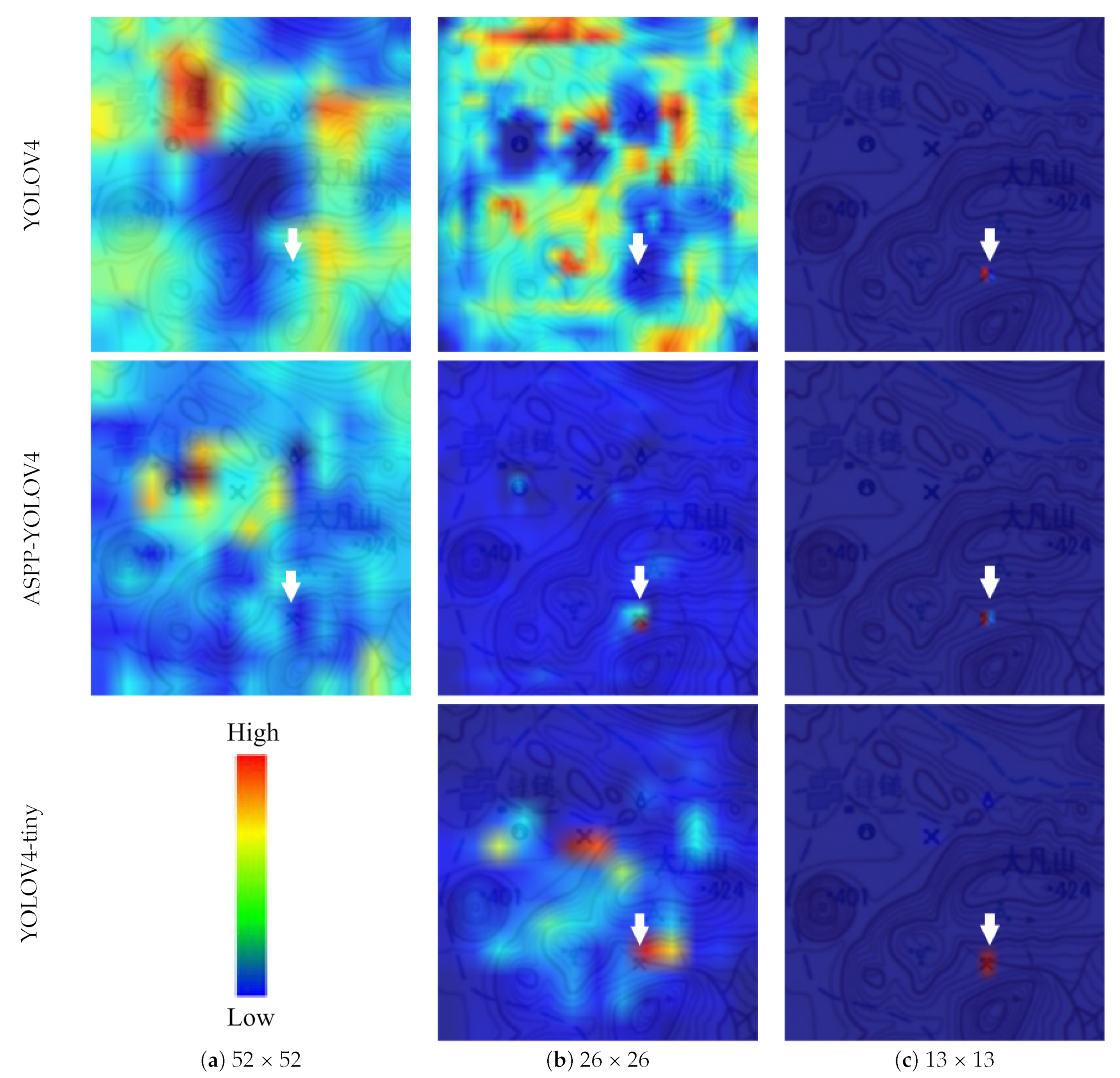
4.2. Feature Analysis Based on Gradient-Weighted Class Activation Mapping (Grad-CAM)

Deep learning is often considered a “black box” that lacks interpretability. To obtain more insight into the characteristics of the different models, Grad-CAM [44] was used to visualize the image regions of high interest in the model that contributed the most to the recognition decision. Therefore, we selected point symbol III in Table 1 as the study subject for the experiment. Figure 16 presents a comparison of the Grad-CAM results of three different models using YOLO heads: YOLOv4 [34], ASPP-YOLOv4, and YOLOv4-tiny [35]. The experimental results and analysis are presented below.

Compared with the YOLOv4 model, the ASPP-YOLOv4 model had a more concentrated area of interest in the symbol characteristics, particularly at the 52 × 52 and 26 × 26 scales. YOLOv4 did not effectively capture regions of interest at these two scales. In the case of YOLOv4-tiny, although only two heads are used for prediction, it is possible to precisely focus on symbolic features for small-scale symbolic targets. However, it deviated when the mesoscale prediction was concentrated on another symbol of a similar shape; hence, it was not as good as ASPP-YOLOV4 for capturing the valid area. This indicates the advantage of the ASPP structure, wherein the model obtains contextual information near the symbol by enlarging the receptive field, allowing the effective capture of the target symbol. Among the three different feature scales, the large-scale learns a large range of features, which is more conducive to global feature extraction, while the small-scale focuses on the features of the task, which aids in learning local features. Through the fusion of global and local semantic information, richer spatial contextual information is obtained for symbol target recognition, effectively improving the symbol recognition accuracy.

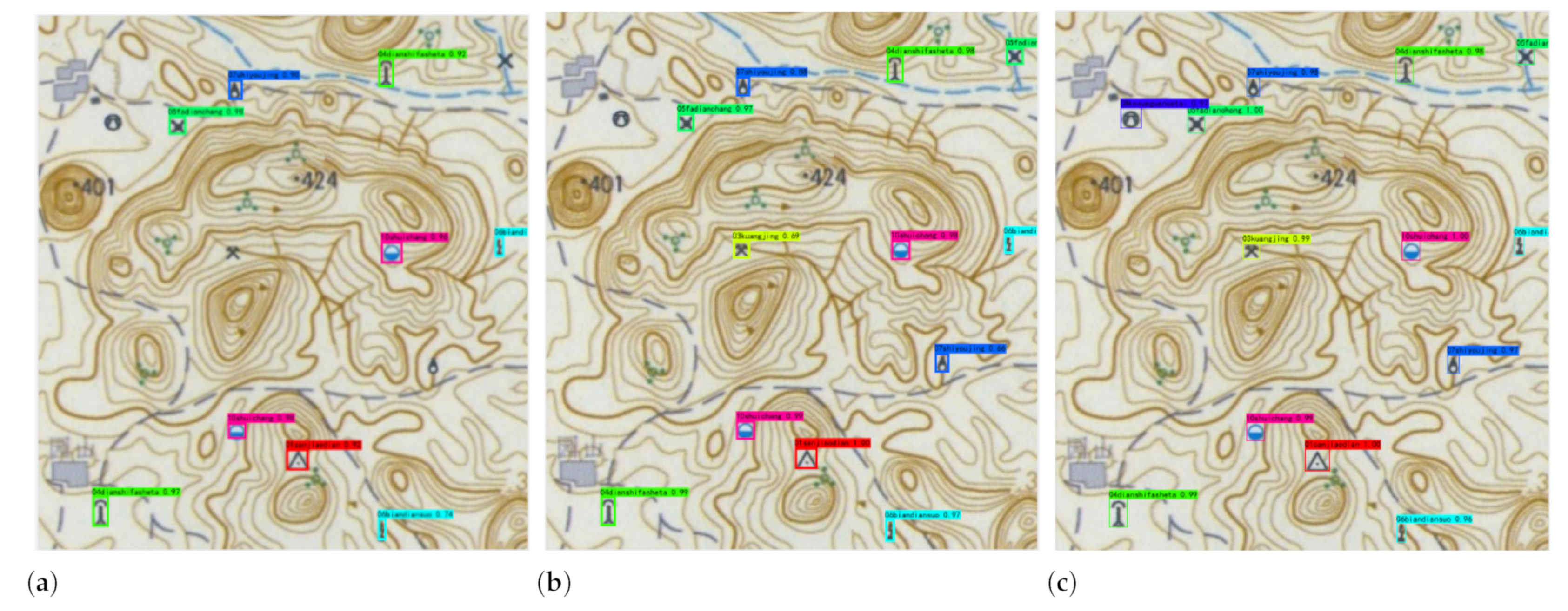
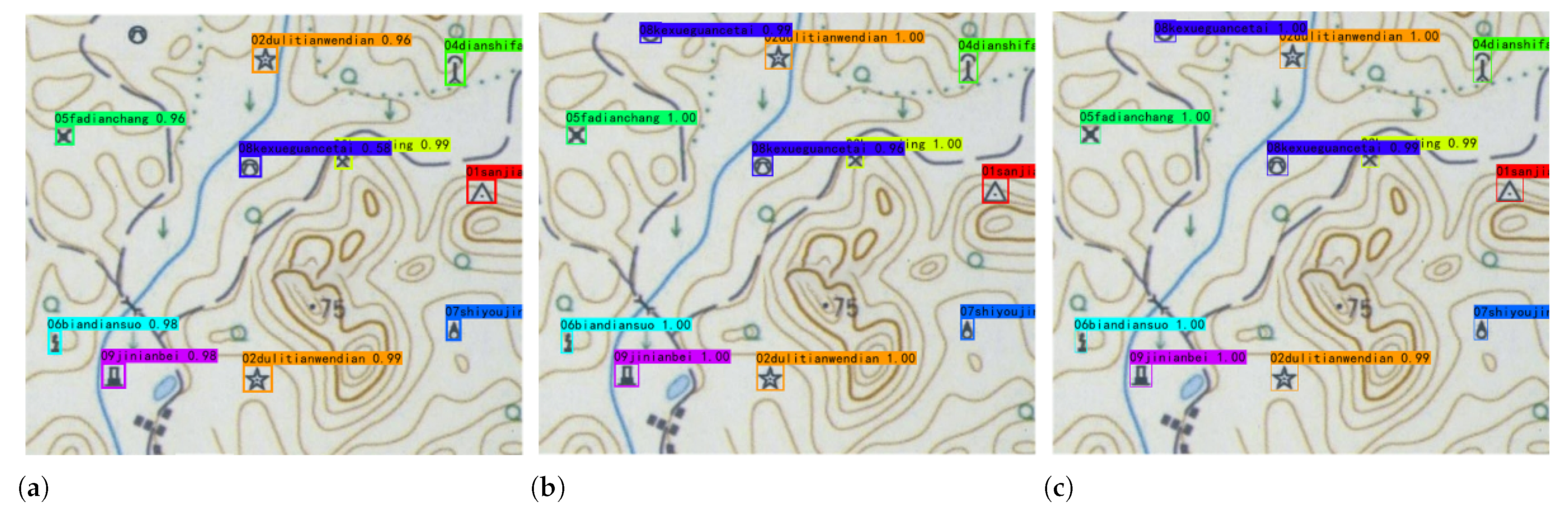
4.3. Comparison of Different Input Image Scales

To further demonstrate the feasibility of the proposed model, experiments were performed with different input image sizes: 320 × 320, 512 × 512, and 640 × 640 pixels. As shown in

Table 4. Performance of ASPP-YOLOv4 model with different input scales.

Input Sizel	Precision	Recall	F1 Score	mAP	MACs(G)	Inference Time (ms)
$320\times 320$	97.53	89.26	93.29	97.04	37.92	47.66
$512\times 512$	98.05	92.89	95.32	97.86	97.06	62.88
$640\times 640$	98.67	94.01	96.46	98.24	151.66	73.18

, when the image scale increased, the recognition performance of ASPP-YOLOv4 improved to a certain extent. The images at these three scales were identified by the model with mAPs of 97.04%, 97.86%, and 98.24%. However, as the image scale increased, the multiply accumulate operations (MACs) of the model also increased. The MAC increased from 18.9 to 75.8 as both the image width and height were increased from 320 to 640 pixels, and ASPP-YOLOv4 required a longer inference time than it did for small-scale images.

Additionally, qualitative experiments were performed to complement the quantitative results, as shown in Figure 17 and Figure 18. More symbols are recognized completely and accurately in the image of 640 × 640 pixels than in those at smaller scales, and the confidence is also higher. As shown in Figure 17a, the proposed model incorrectly recognized four point symbols; a symbol is missing in Figure 18a. When the input image size was increased to 512 × 512 pixels, only one symbol was not recognized, as shown in Figure 17b. All symbols of size 640 × 640 were recognized correctly and completely, as shown in Figure 17c and Figure 18c. As the input size increased, the position of the prediction box moved closer to the smallest bounding rectangle of the symbol, indicating that the positioning accuracy increased. The worst positional results were obtained for the image of 320 × 320 pixels, whereas better results were obtained for images of 512 × 512 and 640 × 640 pixels, as shown in Figure 17 and Figure 18, respectively.

The experimental results indicated that a larger image scale corresponded to a higher point symbol recognition accuracy. In engineering applications, we must balance the recognition accuracy and the detection speed to select the appropriate input image size.

According to these results, we expect that more GPU memory will be consumed for recognizing point symbols in large-scale maps. Therefore, a new method was developed for recognizing point symbols in large-scale maps that achieves better results in less time. We designed the image processing operation of “first cut, then zoom, detect, and finally stitch”, as shown in Figure 19. The entire STM was cropped to a size of 208 × 208 pixels, and zeros were filled in the width and height directions for the undersized part. The resulting images were enlarged two times to 416 × 416 pixels for use as input images. The categories and coordinates of the detected symbols were individually recognized by ASPP-YOLOV4, and then recorded and stored. Finally, the images were stitched together and coordinate conversion was performed. The recognition results were plotted and output.

This method was applied for symbol recognition in large-scale maps, and the results are shown in Figure 20, with a scale of 1241 × 955 pixels. All target symbols in these large-scale maps were recognized completely and accurately. Moreover, all target symbols, except one in the image that was skewed during scanning, were also accurately recognized, as shown in Figure 20b. Clearly, the proposed method is superior to the method of compressing images to a single size for recognition, which requires more computation. Therefore, the proposed method can be used in practical applications.

4.4. Classical Algorithms versus Learning-Based Models for Point Symbol Recognition

As described in Section 3, the ASPP-YOLOv4 method autonomously and comprehensively learns image features and directly outputs the categories and coordinates of the target symbols. The traditional approach for point symbol recognition involves color segmentation of the map followed by manual extraction of the areas around the symbols. Subsequently, template matching [15] or generalized Hough transform (GHT) [12] based on manually defined rules is used to recognize point symbols on the STMs. The experimental results of these algorithms are shown in Figure 21. It was concluded that classical algorithms face the following problems:

•

Long runtime for point symbol recognition. The existing methods require denoising and preprocessing of the map before the recognition of point symbols; next, the image must be segmented to extract possible target areas, which is time-consuming. Moreover, the point symbols may be erreneously removed during preprocessing. However, the proposed deep learning method comprises an end-to-end process, wherein the input RGB images go through the model to directly obtain recognition results, and good recognition performance is achieved. Moreover, the proposed method recognizes multiple point symbols simultaneously, overcoming the limitation of existing methods that individually recognize symbols. The inference times for different methods are presented in

Table 5. The inference time of different methods.

The Maps	Size	Template Matching (s)	GHT (s)	Ours (s)
1	1110 × 738	0.965	4.431	0.085
2	504 × 484	0.453	1.730	0.057
3	389 × 385	0.418	1.670	0.049

.

•

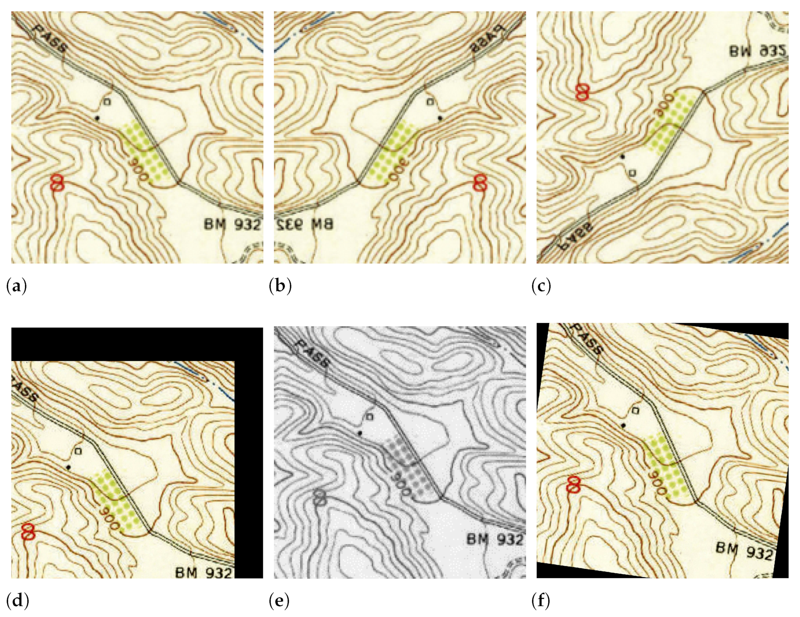
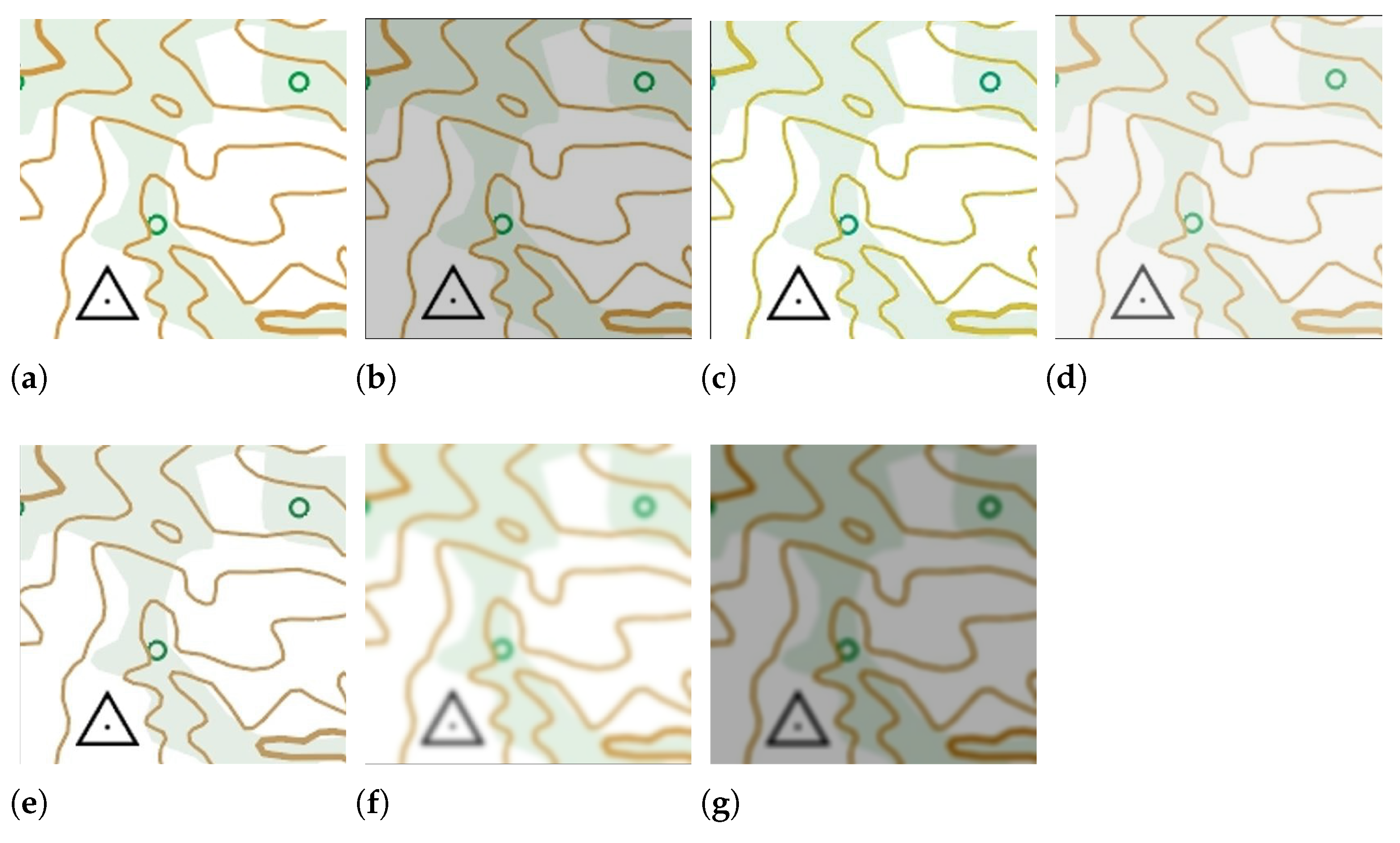
Relatively poor generalization capability. The conventional method can detect point symbols of the same color, size, orientation, and shape. If the paper TM is tilted during scanning, the recognition performance may be poor. As shown in Figure 22, assuming that the size, orientation, shape, or background of the symbols on the map change slightly, the point symbols may not be accurately recognized. In contrast, as described in Section 4, Parts C and E, the proposed model can accurately recognize point symbols that are rotated, scaled, or derived from different basemaps. Therefore, the proposed method has a good generalization capability.

•

Complexity of manually defined rules. Point symbols are approximated as comprising line elements, based on the skeleton information of the symbols, and artificially defined rules are represented in the parameter space to recognize point symbols. When symbols consist of multiple graphical elements, it is difficult to represent them accurately. Thus, the classical algorithms are unstable and highly complex.

4.5. Ablation Experiments

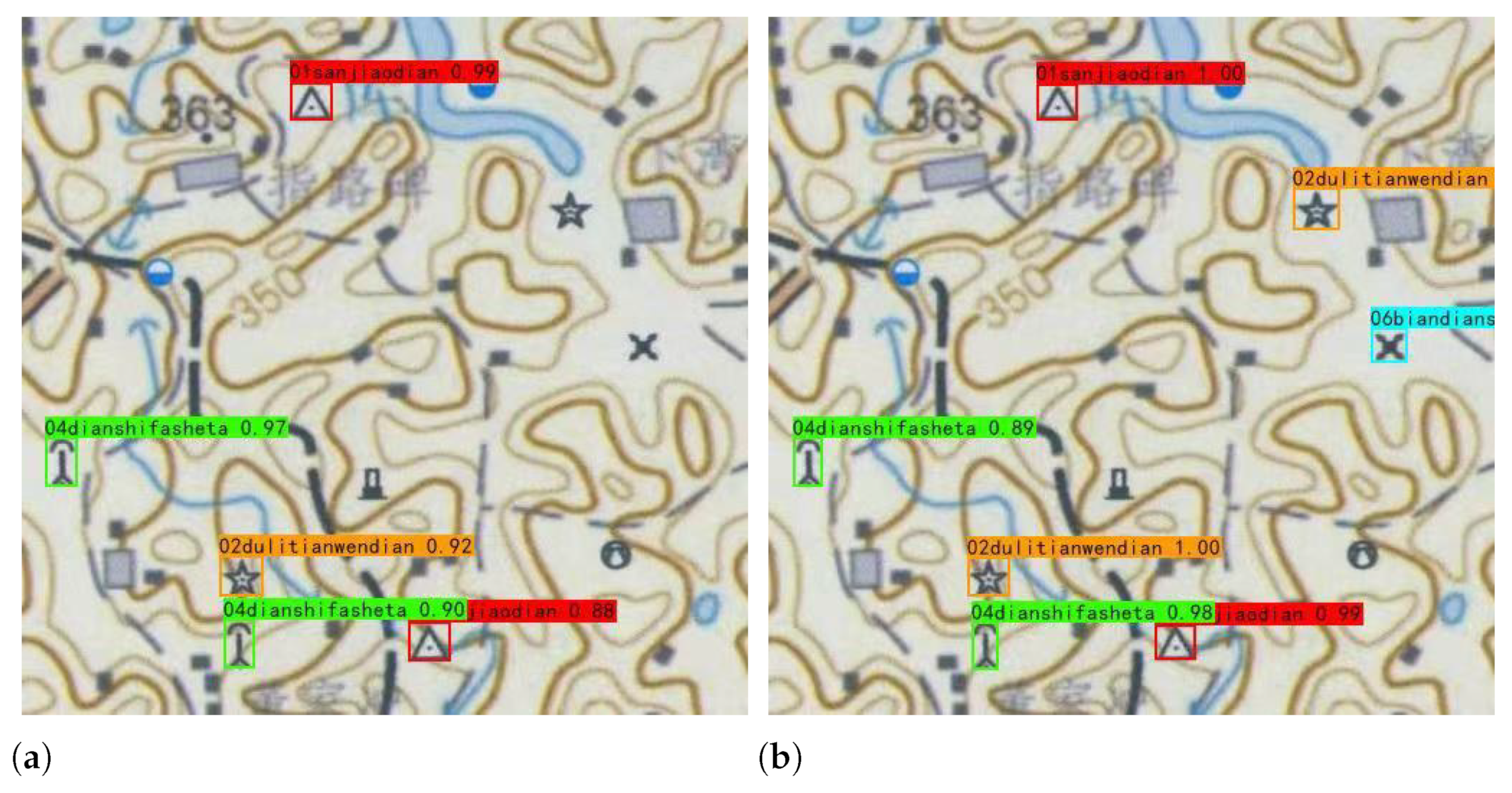
4.5.1. Direct Transfer Learning from Vector-Map to Scanned Map via Gaussian Blur and Color Jitter Augmentation

To evaluate the generalization ability of the proposed method for different map styles, ablation experiments were performed on our scanned map test set using a model trained on the vectorized map dataset containing different map styles. We expected the differences between the training and test sets to make it difficult for the model to accurately capture the target symbol. As shown in

Table 6. Recognition results of a model trained on a vectorized map dataset for our scanned map test set and whether the Gaussian blur combined with color jitter augmentation was used during training.

Gaussian Blur Combined with Color Jitter Method	Precision	Recall	F1 Score	mAP
×	97.10	48.05	58.10	76.40
√	96.72	65.61	74.43	80.09

, the recall for recognition was only 48.05%; therefore, the Gaussian blur must be combined with the color jitter method to transform the vectorized map into a scanned map. The experimental results indicated a significant improvement in the recognition accuracy via the transfer learning strategy, with increases of 17.56%, 16.33%, and 3.69% in the recall, F1 score, and mAP, respectively. However, a significant increase in the recall indicates that the model can recognize more symbols, to the extent that the accuracy decreases slightly. Overall, this method allowed the model to better recognize point symbols, as shown in Figure 23, with fewer missed symbols and a higher confidence. However, the 65.61% recall and 80.09% mAP for the vectorized map dataset indicate that the generalization ability must be improved.

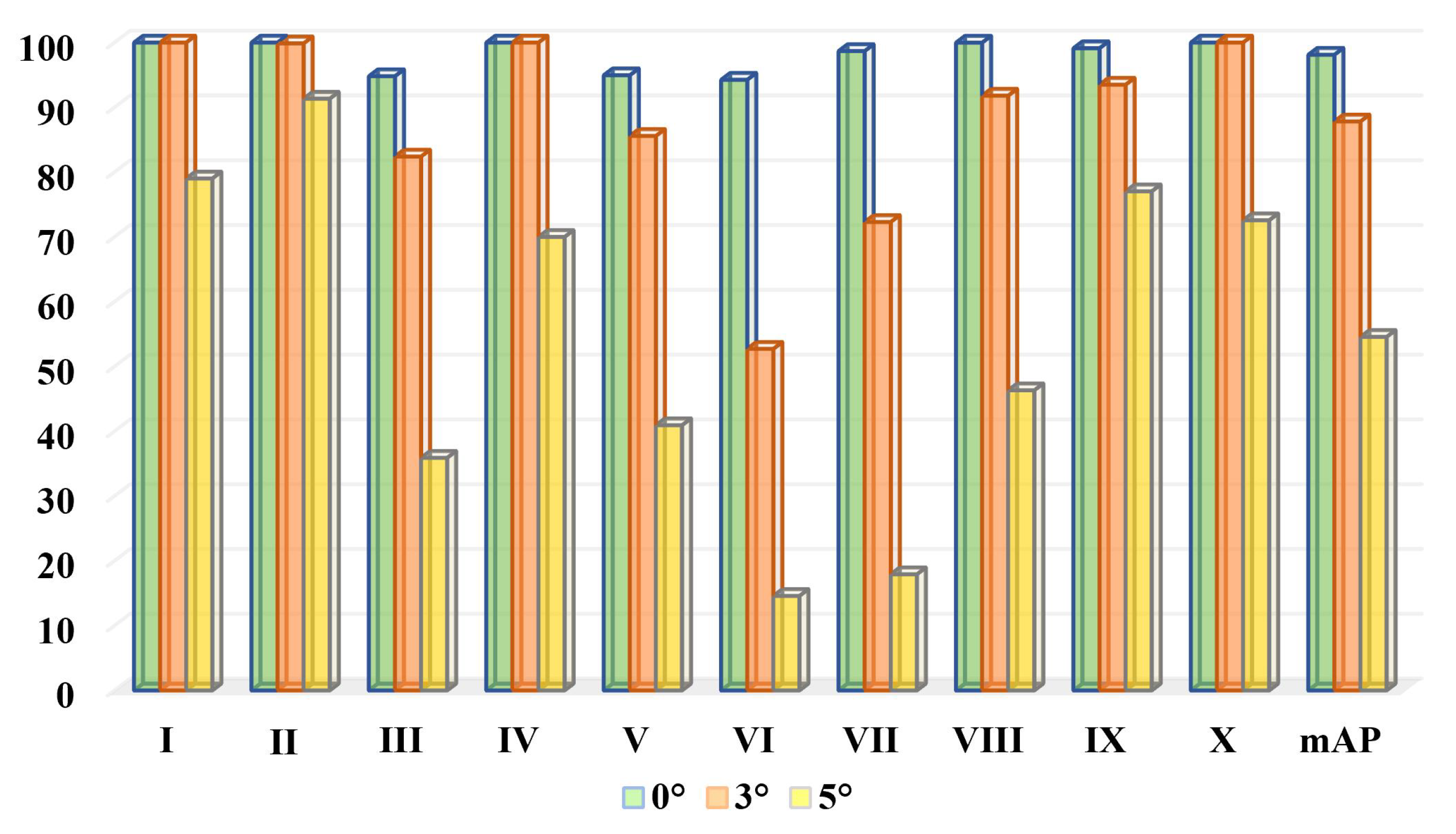
4.5.2. Improve Model Rotation Robustness via Small-Angle Rotation Data Augmentation

During TM scanning, the map may be unaligned (Figure 17a), which affects the symbol-recognition results. The images in the test set were rotated by 3° and 5° to simulate a small-angle tilt of the scanned map, and the experimental results are presented in Figure 24. As shown in the graph, the AP for the symbols in categories III, V, VI, and VII decreased significantly, indicating that these categories were less rotationally robust. The results shown in Figure 25 are consistent with the statistical results: symbols III, VI, and VII were not correctly identified in Map I, which was rotated by 2.5° and 5°, whereas the other symbols in the map were correctly recognized. This was due to the structural characteristics of the point symbols, which are more robust when they are composed of circles or triangles.

To improve the rotational robustness of the model, we applied a data-augmentation method of small-angle rotation with an affine transformation to the training set. A range of 10° clockwise and counterclockwise rotations was set for the training set, and the obtained model was used to recognize our test set rotated by 5°. The experimental results are presented in

Table 7. Comparison of the results based on whether the small-angle rotation data-augmentation method was used during training, which was tested on our test set rotated by 5°.

Small-Angle Rotation	AP										mAP
Data Augmentation Method	I	II	III	IV	V	VI	VII	VIII	IX	X
×	79.01	91.33	35.90	69.99	40.93	14.58	17.92	46.32	77.03	72.56	54.56
√	100.0	99.74	92.63	99.91	92.22	88.32	93.38	92.96	99.88	100.0	95.90

. As shown, the mAP was significantly increased by this data-augmentation method, and a good AP was obtained for all types of symbols. Thus, the poor rotation robustness was addressed, improving the generalization of the model and its applicability in engineering.

5. Conclusions

In this study, the ASPP-YOLOv4 model was designed with a modified YOLOv4 framework, which was used to predict the categories and locations of point symbols on STMs. Compared with four classical detectors (faster R-CNN, VGG-SSD, YOLOv3, and YOLOv4) and two state-of-the-art methods (template matching and GHT), the proposed method focuses more on the target area, as indicated by the Grad-CAM visualization. It achieved significantly higher recognition and positioning accuracies (mAP of 98.11% and mIoU of 0.876), ranking first among all the methods. Additionally, considering the limited GPU memory and runtime, a cut-stitch method was developed for recognizing large-scale maps. The feasibility of this approach was demonstrated by the fact that all the target symbols in two large-scale maps were promptly and accurately recognized. Furthermore, the model was shown to have strong generalization ability. It can recognize point symbols that are rotated, scaled, or derived from different basemaps, addressing the limitations of existing methods.

Although the proposed ASPP-YOLOv4 model achieved good performance in point symbol recognition, it has several limitations. As indicated by the arrows in Figure 20b, the same symbol was recognized twice, because the symbols are exactly tessellated when cropping a large image. Therefore, the cut-stitch approach must allow further screening of the recognition results. Second, if the paper TM is folded during scanning, some point symbols on the STM may be distorted. In this case, the positioning of all symbols is incorrect because of the map folding, which results in the offset of the geographic feature coordinates after map vectorization. If the paper TM is folded during scanning, it must be rescanned. Finally, we focused on STM images, and the objects and results of the processing were image data, whereas the result of point symbol recognition is obtained as vectorized data. Therefore, converting existing results into vectorized data will be the focus of future work.

Another problem was that in the dataset used in this study, the point symbols all pointed to the north and had a regular structure, but the TM also contained undirected symbols. Our model needs advanced algorithms, such as rotation invariance, to solve the problem of undirected symbol recognition. Moreover, only a few point symbols are distributed on the STM, and those in some maps cannot be publicly published. Therefore, only 10 common point symbols were included in our dataset, as shown in Table 1. However, TMs contain more types of symbols; therefore, we will collect more samples of point symbols to enrich the dataset in a future study. Thus, we will provide sufficient data to support the digital production of STMs.

References

1. Liu, T.; Xu, P.; Zhang, S. A review of recent advances in scanned topographic map processing. Neurocomputing 2019, 328, 75–87. [Google Scholar] [CrossRef]
2. Lin, S.S.; Lin, C.H.; Hu, Y.J.; Lee, T.Y. Drawing Road Networks with Mental Maps. IEEE Trans. Vis. Comput. Graph. 2014, 20, 1241–1252. [Google Scholar] [CrossRef] [PubMed] [Green Version]
3. Lladós, J.; Valveny, E.; Sánchez, G.; Marti, E. Symbol Recognition: Current Advances and Perspectives. In Proceedings of the International Workshop on Graphics Recognition, Kingston, ON, Canada, 7–8 September 2001; pp. 104–128. [Google Scholar]
4. Uhl, J.H.; Leyk, S.; Chiang, Y.Y.; Knoblock, C.A. Towards the automated large-scale reconstruction of past road networks from historical maps. Comput. Environ. Urban Syst. 2022, 94, 101794. [Google Scholar] [CrossRef]
5. Burghardt, K.; Uhl, J.H.; Lerman, K.; Leyk, S. Road network evolution in the urban and rural United States since 1900. Comput. Environ. Urban Syst. 2022, 95, 101803. [Google Scholar] [CrossRef]
6. Leyk, S.; Chiang, Y.Y. Information extraction based on the concept of geographic context. In Proceedings of the AutoCarto 2016, Reston, VI, USA, 9–11 December 2016; pp. 100–110. [Google Scholar]
7. Khan, I.; Islam, N.; Ur Rehman, H.; Khan, M. A comparative study of graphic symbol recognition methods. Multimed. Tools Appl. 2020, 79, 8695–8725. [Google Scholar] [CrossRef]
8. Song, J.; Zhang, Z.; Qi, Y.; Miao, Q. Point Symbol Recognition Algorithm based on Improved Generalized Hough Transform and Nonlinear Mapping. In Proceedings of the 2018 International Conference on Security, Pattern Analysis, and Cybernetics (SPAC), Jinan, China, 14–18 December 2018; pp. 134–139. [Google Scholar]
9. Nass, A.; Gasselt, S.v. Dynamic Cartography: A Concept for Multidimensional Point Symbols. In Progress in Cartography; Springer: Berlin/Heidelberg, Germany, 2016; pp. 17–30. [Google Scholar]
10. Leyk, S.; Boesch, R. Colors of the past: Color image segmentation in historical topographic maps based on homogeneity. GeoInformatica 2010, 14, 1–21. [Google Scholar] [CrossRef]
11. Szendrei, R.; Elek, I.; Márton, M. A knowledge-based approach to raster-vector conversion of large scale topographic maps. Acta Cybern. 2011, 20, 145–165. [Google Scholar] [CrossRef]
12. Camassa, R.; Kuang, D.; Lee, L. A geodesic landmark shooting algorithm for template matching and its applications. SIAM J. Imaging Sci. 2017, 10, 303–334. [Google Scholar] [CrossRef] [Green Version]
13. Shen, J.; Du, Y.; Wang, W.; Li, X. Lazy random walks for superpixel segmentation. IEEE Trans. Image Process. 2014, 23, 1451–1462. [Google Scholar] [CrossRef]
14. Tian, F.; Wei, R.; Ding, Q.; Xiong, L. New approach for oil-well symbol recognition in petroleum geological structure map. In Proceedings of the 2010 International Conference on Electrical and Control Engineering, Wuhan, China, 25–27 June 2010; pp. 5357–5360. [Google Scholar]
15. Miao, Q.; Xu, P.; Li, X.; Song, J.; Li, W.; Yang, Y. The Recognition of the Point Symbols in the Scanned Topographic Maps. IEEE Trans. Image Process. 2017, 26, 2751–2766. [Google Scholar] [CrossRef]
16. Reiher, E.; Li, Y.; Delle Donne, V.; Lalonde, M.; Hayne, C.; Zhu, C. A system for efficient and robust map symbol recognition. In Proceedings of the 13th International Conference on Pattern Recognition, Washington, DC, USA, 25–29 August 1996; Volume 3, pp. 783–787. [Google Scholar]
17. Pezeshk, A.; Tutwiler, R.L. Automatic Feature Extraction and Text Recognition From Scanned Topographic Maps. IEEE Trans. Geosci. Remote Sens. 2011, 49, 5047–5063. [Google Scholar] [CrossRef]
18. Pezeshk, A.; Tutwiler, R. Extended character defect model for recognition of text from maps. In Proceedings of the 2010 IEEE Southwest Symposium on Image Analysis & Interpretation (SSIAI), Austin, TX, USA, 23–25 May 2010; pp. 85–88. [Google Scholar] [CrossRef]
19. Pezeshk, A.; Tutwiler, R.L. Improved Multi Angled Parallelism for separation of text from intersecting linear features in scanned topographic maps. In Proceedings of the 2010 IEEE International Conference on Acoustics, Speech and Signal Processing, Dallas, TX, USA, 14–19 March 2010; pp. 1078–1081. [Google Scholar]
20. Zhou, X.; Wang, D.; Krähenbühl, P. Objects as points. arXiv 2019, arXiv:1904.07850. [Google Scholar]
21. Ren, S.; He, K.; Girshick, R.; Sun, J. Faster r-cnn: Towards real-time object detection with region proposal networks. arXiv 2015, arXiv:1506.01497v3. [Google Scholar] [CrossRef] [PubMed] [Green Version]
22. Qiu, C.; Li, H.; Guo, W.; Chen, X.; Yu, A.; Tong, X.; Schmitt, M. Transferring transformer-based models for cross-area building extraction from remote sensing images. IEEE J. Sel. Top. Appl. Earth Obs. Remote Sens. 2022, 15, 4104–4116. [Google Scholar] [CrossRef]
23. Li, S.; Liao, C.; Ding, Y.; Hu, H.; Jia, Y.; Chen, M.; Xu, B.; Ge, X.; Liu, T.; Wu, D. Cascaded Residual Attention Enhanced Road Extraction from Remote Sensing Images. ISPRS Int. J.-Geo-Inf. 2021, 11, 9. [Google Scholar] [CrossRef]
24. Cheng, G.; Zhou, P.; Han, J. Learning rotation-invariant convolutional neural networks for object detection in VHR optical remote sensing images. IEEE Trans. Geosci. Remote Sens. 2016, 54, 7405–7415. [Google Scholar] [CrossRef]
25. Rahimzadegan, M.; Sadeghi, B. Development of the iterative edge detection method applied on blurred satellite images: State of the art. J. Appl. Remote Sens. 2016, 10, 035018. [Google Scholar] [CrossRef]
26. Rahimzadegan, M.; Sadeghi, B.; Masoumi, M.; Taghizadeh Ghalehjoghi, S. Application of target detection algorithms to identification of iron oxides using ASTER images: A case study in the North of Semnan province, Iran. Arab. J. Geosci. 2015, 8, 7321–7331. [Google Scholar] [CrossRef]
27. Zhang, P.; Gong, M.; Su, L.; Liu, J.; Li, Z. Change detection based on deep feature representation and mapping transformation for multi-spatial-resolution remote sensing images. ISPRS J. Photogramm. Remote Sens. 2016, 116, 24–41. [Google Scholar] [CrossRef]
28. LeCun, Y.; Bottou, L.; Bengio, Y.; Haffner, P. Gradient-Based Learning Applied to Document Recognition; IEEE: Hoboken, NJ, USA, 1998; Volume 86, pp. 2278–2324. [Google Scholar]
29. Quan, Y.; Shi, Y.; Miao, Q.; Qi, Y. A combinatorial solution to point symbol recognition. Sensors 2018, 18, 3403. [Google Scholar] [CrossRef] [PubMed] [Green Version]
30. Guo, M.; Bei, W.; Huang, Y.; Chen, Z.; Zhao, X. Deep learning framework for geological symbol detection on geological maps. Comput. Geosci. 2021, 157, 104943. [Google Scholar] [CrossRef]
31. Kim, H.; Lee, W.; Kim, M.; Moon, Y.; Lee, T.; Cho, M.; Mun, D. Deep-learning-based recognition of symbols and texts at an industrially applicable level from images of high-density piping and instrumentation diagrams. Expert Syst. Appl. 2021, 183, 115337. [Google Scholar] [CrossRef]
32. Zhao, Z.Q.; Zheng, P.; Xu, S.t.; Wu, X. Object detection with deep learning: A review. IEEE Trans. Neural Netw. Learn. Syst. 2019, 30, 3212–3232. [Google Scholar] [CrossRef] [PubMed] [Green Version]
33. Redmon, J.; Farhadi, A. Yolov3: An incremental improvement. arXiv 2018, arXiv:1804.02767. [Google Scholar]
34. Bochkovskiy, A.; Wang, C.Y.; Liao, H.Y.M. Yolov4: Optimal speed and accuracy of object detection. arXiv 2020, arXiv:2004.10934. [Google Scholar]
35. Liu, Q.; Fan, X.; Xi, Z.; Yin, Z.; Yang, Z. Object detection based on Yolov4-Tiny and Improved Bidirectional feature pyramid network. J. Phys. Conf. Ser. 2022, 2209, 012023. [Google Scholar] [CrossRef]
36. Liu, W.; Anguelov, D.; Erhan, D.; Szegedy, C.; Reed, S.; Fu, C.Y.; Berg, A.C. Ssd: Single shot multibox detector. In Proceedings of the European Conference on Computer Vision, Amsterdam, The Netherlands, 8–10 October 2016; pp. 21–37. [Google Scholar]
37. Chen, C.; Zhong, J.; Tan, Y. Multiple-oriented and small object detection with convolutional neural networks for aerial image. Remote Sens. 2019, 11, 2176. [Google Scholar] [CrossRef] [Green Version]
38. Chen, L.; Shi, W.; Deng, D. Improved YOLOv3 based on attention mechanism for fast and accurate ship detection in optical remote sensing images. Remote Sens. 2021, 13, 660. [Google Scholar] [CrossRef]
39. Li, G.; Xie, H.; Yan, W.; Chang, Y.; Qu, X. Detection of road objects with small appearance in images for autonomous driving in various traffic situations using a deep learning based approach. IEEE Access 2020, 8, 211164–211172. [Google Scholar] [CrossRef]
40. Chen, L.C.; Papandreou, G.; Schroff, F.; Adam, H. Rethinking atrous convolution for semantic image segmentation. arXiv 2017, arXiv:1706.05587. [Google Scholar]
41. Wang, P.; Chen, P.; Yuan, Y.; Liu, D.; Huang, Z.; Hou, X.; Cottrell, G. Understanding convolution for semantic segmentation. In Proceedings of the 2018 IEEE Winter Conference on Applications of Computer Vision (WACV), Lake Tahoe, NV, USA, 12–15 March 2018; pp. 1451–1460. [Google Scholar]
42. He, K.; Zhang, X.; Ren, S.; Sun, J. Spatial pyramid pooling in deep convolutional networks for visual recognition. IEEE Trans. Pattern Anal. Mach. Intell. 2015, 37, 1904–1916. [Google Scholar] [CrossRef] [PubMed] [Green Version]
43. Angeles, J.; Pasini, D. Affine Transformations. In Fundamentals of Geometry Construction: The Math Behind the CAD; Springer International Publishing: Cham, Switzerland, 2020; pp. 103–163. [Google Scholar] [CrossRef]
44. Selvaraju, R.R.; Cogswell, M.; Das, A.; Vedantam, R.; Parikh, D.; Batra, D. Grad-cam: Visual explanations from deep networks via gradient-based localization. In Proceedings of the IEEE International Conference on Computer Vision, Venice, Italy, 22–29 October 2017; pp. 618–626. [Google Scholar]
Figure 1. Examples of point symbols on the 1955 STM of Grand Island. (a,b) are locally enlarged maps with point symbols. Map source: USGS-HTMC.
Ijgi 12 00128 g001
Figure 2. Number statistical results for the training set and total set of the scanned map dataset.
Ijgi 12 00128 g002
Figure 3. Three annotation samples of the scanned map dataset.
Ijgi 12 00128 g003
Figure 4. Statistical results for the entire vectorized map dataset.
Ijgi 12 00128 g004
Figure 5. Three annotation samples of the vectorized map dataset.
Ijgi 12 00128 g005
Figure 6. Annotation samples of the PASCAL VOC dataset, which is mainly used for natural object detection.
Ijgi 12 00128 g006
Figure 7. Overview of the YOLOv4 framework combined with ASPP. The backbone is composed of the feature extraction network CSPDarknet53, the neck is composed of PANet combined with ASPP, and the three heads are used for prediction.
Ijgi 12 00128 g007
Figure 8. Illustration of the SPP module structure, redrawn according to [41]. Extraction of features using multiple pooling layers at different scales and fusion into a 21-dimensional vector input for the fully connected layer.
Ijgi 12 00128 g008
Figure 9. Illustration of the proposed ASPP module structure comprising multiple parallel levels: A 1 × 1 convolution; three 3 × 3 dilated convolutions with dilation rates of 1, 3, 5, respectively; and image pooling.
Ijgi 12 00128 g009
Figure 10. Images obtained by applying the data augmentation methods to the original image (a): (b) with a horizontal flip, (c) with vertical flipping, (d) with cropping, (e) ToGray, and (f) by rotating at a small angle.
Ijgi 12 00128 g010
Figure 11. Images obtained by applying the Gaussian blur combined with color jitter method to the original image (a): (b) brightness transformation, (c) hue transformation, (d) contrast transformation, (e) saturation transformation, (f) Gaussian blur, and (g) Gaussian blur combined with color jitter.
Ijgi 12 00128 g011
Figure 12. Statistical plots of the AP values of the ten point symbols in Table 1 identified using different models.
Ijgi 12 00128 g012
Figure 13. Results obtained by different models for Map A: (a) faster R-CNN, (b) VGG-SSD, (c) YOLOv3, (d) YOLOv4, and (e) ASPP-YOLOv4.
Ijgi 12 00128 g013
Figure 14. Results obtained by different models for Map B: (a) faster R-CNN, (b) VGG-SSD, (c) YOLOv3, (d) YOLOv4, and (e) ASPP-YOLOv4.
Ijgi 12 00128 g014
Figure 15. Results obtained by different models for Map C: (a) faster R-CNN, (b) VGG-SSD, (c) YOLOv3, (d) YOLOv4, and (e) ASPP-YOLOv4.
Ijgi 12 00128 g015
Figure 16. Comparison of Grad-CAM results obtained with YOLO heads of three YOLOv4-based models. Warmer colors indicate higher interest in the area, whereas cooler colors indicate the opposite; the white arrow points to the object of the study, the point symbol III.
Ijgi 12 00128 g016
Figure 17. Results obtained for different input image sizes of Map D: (a) 320 × 320, (b) 512 × 512, and (c) 640 × 640 pixels.
Ijgi 12 00128 g017
Figure 18. Results obtained for different input image sizes of Map E: (a) 320 × 320, (b) 512 × 512, and (c) 640 × 640 pixels.
Ijgi 12 00128 g018
Figure 19. Symbol detection processing operation for large-scale maps: “first cut, then zoom, detect, and finally stitch”.
Ijgi 12 00128 g019
Figure 20. Results obtained by the proposed ASPP-YOLOv4 for Map F of size 1241 × 955 pixels. (a) Original image and (b) the image skewed during scanning. The red circle indicates missed recognition.
Ijgi 12 00128 g020
Figure 21. Recognition results of different methods for Map G. (a) Results of Template matching. (b) Results of GHT. (c) Results of the proposed ASPP-YOLOv4. In (a,b), the green box indicates correct recognition, whereas the red circle indicates missed recognition.
Ijgi 12 00128 g021
Figure 22. Symbol recognition results of template matching method for different scenes. The green box indicates correct recognition, whereas the red circle indicates missed recognition. (a) Template. (b) Results for different map backgrounds. (c) Results for 0.8 times smaller size. (d) Results for 5° angle rotation.
Ijgi 12 00128 g022
Figure 23. Recognition results of the model trained on the vectorized map dataset for the scanned Map H. (a) Recognition results without the Gaussian blur and color jitter data augmentation method. (b) Recognition results with the Gaussian blur and color jitter data augmentation method.
Ijgi 12 00128 g023
Figure 24. Statistical plots of different rotation angles on our test set.
Ijgi 12 00128 g024
Figure 25. Recognition results for different rotation angles of Map I: (a) original image, (b) rotated by 2.5°, and (c) rotated by 5°.
Ijgi 12 00128 g025