Article

Generating Gridded Gross Domestic Product Data for China Using Geographically Weighted Ensemble Learning

1
College of Hydrology and Water Resources, Hohai University, Nanjing 210098, China
2
Flood and Drought Disaster Prevention and Protection Center of Heilongjiang Province, Haerbin 150006, China
3
Research Center on Flood and Drought Disaster Reduction, China Institute of Water Resources and Hydropower Research, Beijing 100038, China
*
Author to whom correspondence should be addressed.
ISPRS Int. J. Geo-Inf. 2023, 12(3), 123; https://doi.org/10.3390/ijgi12030123
Submission received: 13 January 2023 / Revised: 1 March 2023 / Accepted: 7 March 2023 / Published: 10 March 2023

Abstract

:
Gridded gross domestic product (GDP) data are a crucial land surface parameter for many geoscience applications. Recently, machine learning approaches have become powerful tools in generating gridded GDP data. However, most machine learning approaches for gridded GDP estimation seldom consider the geographical properties of input variables. Therefore, in this study, a geographically weighted stacking ensemble learning approach was developed to generate gridded GDP data. Three algorithms—random forest, XGBoost, and LightGBM—were used as base models, and the linear regression in stacking ensemble learning was replaced by geographically weighted regression to locally fuse the three predictions. A case study was conducted in China to demonstrate the effectiveness of the proposed approach. The results showed that the proposed GDP downscaling approach outperformed the three base models and traditional stacking ensemble learning. Meanwhile, it had good predictive power on county-level GDP test data with R2 of 0.894, 0.976, and 0.976 for the primary, secondary, and tertiary sectors, respectively. Moreover, the predicted 1 km gridded GDP data had a high accuracy (R2 = 0.787) when evaluated by town-level GDP data. Hence, the proposed GDP downscaling approach provides a valuable option for generating gridded GDP data. The generated 1 km gridded GDP data of China from 2020 are of great significance for other applications.

1. Introduction

Gross domestic product (GDP) is one of the most crucial economic indicators to measure regional economic development status worldwide [1,2,3]. GDP is widely used in discovering economic development inequality, identifying poverty, evaluating disaster risk assessment, and allocating resources [4,5,6,7,8]. Traditional GDP data are often collected through statistical tables of censuses, and they can be spatially linked to administrative boundaries to obtain specific knowledge regarding GDP distribution. However, traditional GDP data are limited by their spatial scale inconsistency with other data and unknown spatial distribution within each administrative unit [2,6,9]. The conversion of traditional GDP data into gridded GDP data (termed as GDP downscaling or GDP spatialization) is a way to address these limitations and enable the application of GDP data to a variety of geoscience fields [3,10,11,12,13,14,15].
GDP downscaling often takes gridded auxiliary data as covariates to improve the quality of gridded GDP data. With the rapid development of remote sensing technology and social sensing technology, various land surface variables can be obtained to reflect up-to-date socioeconomic information [8,16,17,18]. Remote sensing images provide a relatively low-cost way to map the main physical features of our world in a wide range [19,20,21,22]. There are three main categories of remote sensing data in GDP downscaling. Night-time lights (NTL) data, which includes the Defense Meteorological Satellite Program’s Operational Linescan System (DMSP/OLS) and the visible infrared imaging radiometer suite (VIIRS), are often used to generate gridded GDP data [6,13,14]. NTL data have the capability to describe the features in the secondary and tertiary sectors of GDP but limited capability to reflect the attributes in the primary sector of GDP [10,23]. Land cover data extracted from remote sensing images are able to provide spatial distribution information relevant to the primary sector of GDP (e.g., farmland) for estimating gridded GDP [23,24]. Digital elevation model (DEM) and its derived variables (e.g., slope) are also applied to estimate gridded GDP for the primary sector because they are related to the spatial distribution of agricultural activities [10,25]. Although remote sensing data have achieved relatively satisfactory performance in GDP downscaling, they usually fail to capture socioeconomic attributes and human dynamics when estimating gridded GDP [10,16]. Social sensing data have been proven to successfully reflect socioeconomic attributes [8,16]. A variety of social sensing data is used for gridded GDP estimation, such as the density of roads [24], points of interest (POIs) [10], digital footprint of human activities [2], and footprint of buildings [26]. The combined usage of remote sensing data and social sensing data has been a popular way to generate gridded GDP data in recent years [2,10,23,24,25,26,27].
Many GDP downscaling approaches have been developed in recent decades, including traditional statistical methods and machine learning algorithms. Traditional statistical methods contain linear regression [6,13,23], exponential model [9,28], and quadratic polynomial regression [25]. Traditional statistical methods have limited capability to identify the complex relationship between GDP and its relevant auxiliary data. In recent years, machine learning algorithms have been increasingly applied to produce gridded GDP using geospatial big data as they enable data-driven knowledge discovery in relation to GDP [10,11,24,27]. Common machine learning algorithms that have been employed in generating gridded GDP data involve gradient boosting ([24], neural networks [27], and random forest regression [10]. They have demonstrated their capability in exploring the complex relationship between GDP and its related covariates [10,24,27]. Individual machine learning algorithms usually have their merits and shortcomings. Overfitting and instability are critical shortcomings of various machine learning algorithms. A popular way to address these shortcomings is to develop ensemble learning approaches. Ensemble learning intends to fuse the predictions from two or more machine learning algorithms. Ensemble learning involves bagging, boosting, blending, and stacking [29]. Bagging and boosting attempt to combine machine learning algorithms with the same type, whereas blending and stacking aim to integrate different types of machine learning algorithms [7,29]. Blending and stacking can combine not only traditional different types of machine learning algorithms but also the bagging and boosting approaches [7,30,31]. Bagging and boosting fuse the predictions in a relatively simple way (e.g., mean of predictions in regression), while blending and stacking often combine the predictions using global linear regression [7,30,31]. Compared to blending, stacking requires a more robust training mechanism for fusing the predictions, and it often outperforms blending [7,32].
Geospatial variables often demonstrate certain geographical properties [33,34,35,36], such as spatial dependence, spatial heterogeneity, etc. Most of the machine learning algorithms that are used for GDP downscaling seldom consider the geographical properties of the used variables [37,38,39]. Moreover, the fusion of predictions in ensemble learning fails to consider the geographical properties. A spatially local model may be better than a global model in many scenarios [37,38,39]. For instance, Huang et al. [2] used a local model—geographically weighted linear regression model (GWR)—to estimate gridded GDP and proved that GWR performed better than global linear regression. However, GWR only establishes local linear regression for each spatial unit and fails to explore the nonlinear relationship between GDP and its covariates. Thus, given the current GDP downscaling methods lack the combined consideration of the geographical characteristics of input variables and the nonlinear complex relationship between GDP and its covariates, a more effective GDP downscaling method is urgently required.
To fill the above research gaps, this study aimed to develop a geographically weighted stacking ensemble learning approach to locally fuse the predictions of base models using GWR to generate gridded GDP. In this study, a novel geographically weighted stacking ensemble learning approach (GWSE) is proposed for GDP downscaling, which can encapsulate both geographical properties and nonlinear relationship in GDP downscaling. The effectiveness of the proposed GWSE was substantiated by generating 1 km gridded GDP data of China from 2020.

2. Study Area and Data

2.1. Study Area

China has been experiencing rapid economic development and is the second largest economy in the world. Gridded GDP maps therefore have crucial applications nationally. In this study, mainland China with 31 provinces was selected as the study area. Hong Kong, Macao, and Taiwan were excluded because of the difference in currencies.

2.2. Data

Two types of datasets were used in this study. The first type was county-level statistical GDP dataset for the year of 2020 from the 2021 yearbook of China, which was regarded as the dependent variable. The second type was the 1 km gridded auxiliary data, which were considered as covariates (i.e., independent variables).

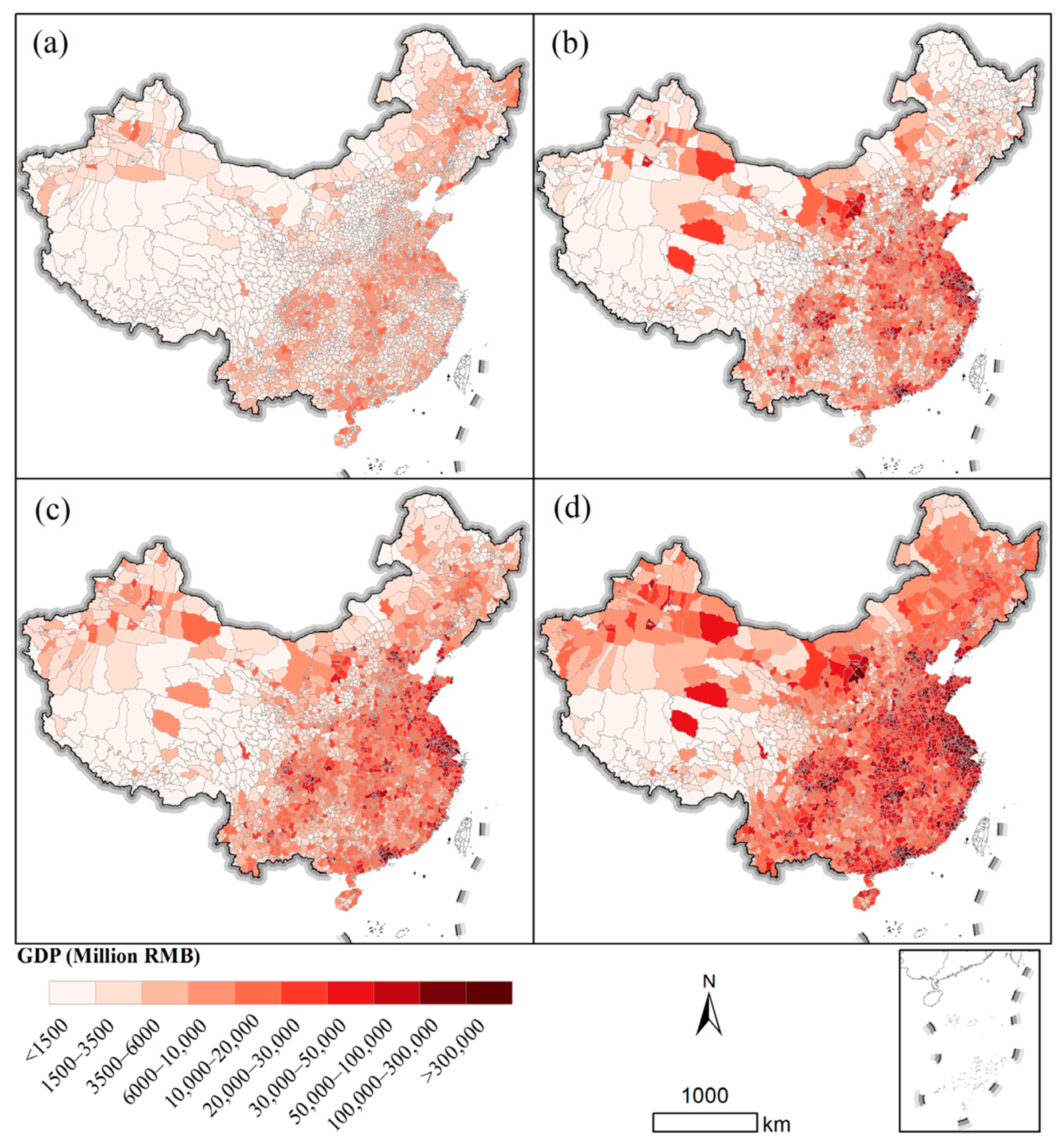
2.2.1. County-Level Statistical GDP Data

The county-level statistical GDP data of 2020 of mainland China were collected to generate the gridded GDP data. Four county-level indicators—the primary sector (GDP1), the secondary sector (GDP2), the tertiary sector (GDP3), and the total GDP—were collected from the 2021 yearbook of China and the 2021 yearbook of provinces in mainland China. Finally, there was a total of 2848 counties with four GDP indicators in mainland China, as shown in Figure 1.

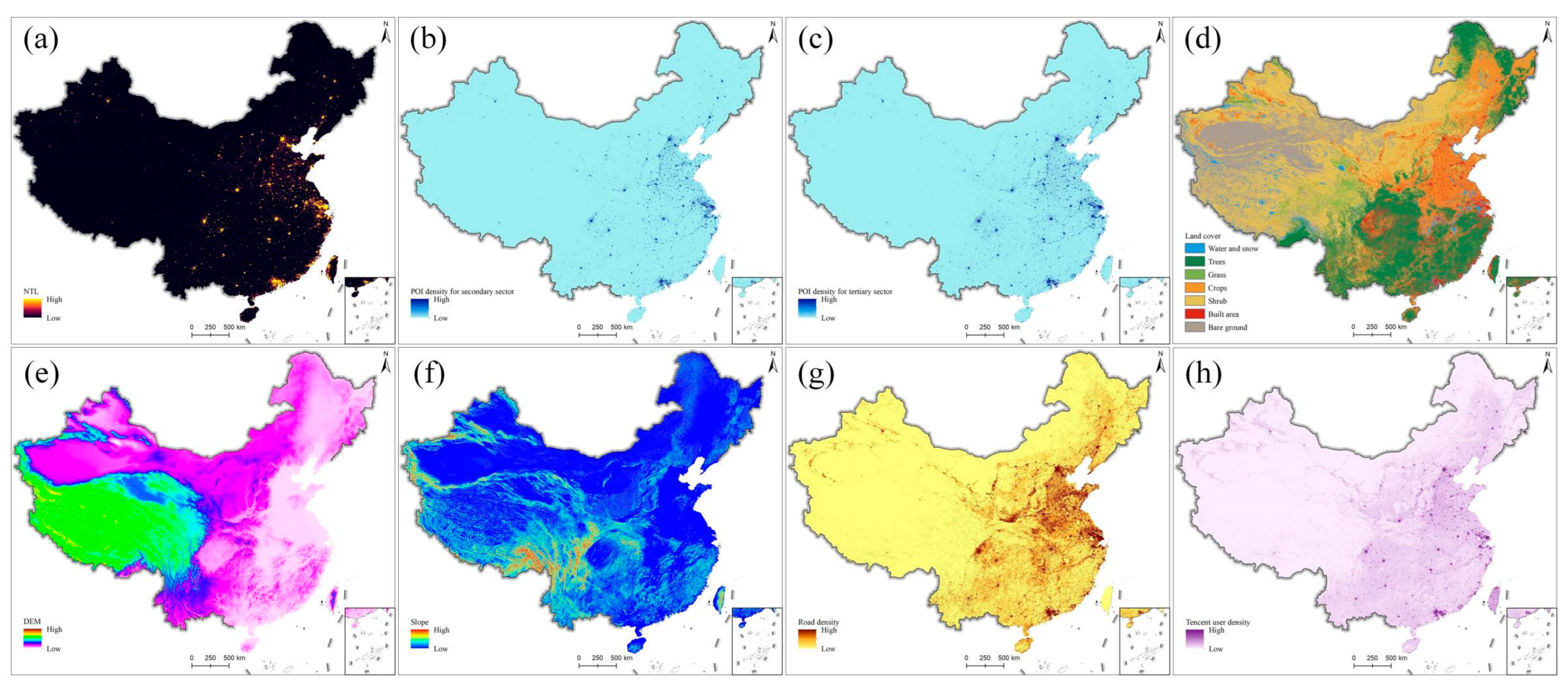
2.2.2. Gridded Auxiliary Data

Auxiliary datasets are essential to generate gridded GDP data in the process of GDP downscaling. Inspired by previous studies [2,10,23,25,27], we collected eight types of 1 km gridded auxiliary data in relation to GDP, as shown in Figure 2.
NTL is widely used for generating gridded GDP as it is related to the secondary and tertiary sectors of GDP. Thus, the annually composited VIIRS NTL image with saturation correction from 2020 was collected [40]. The original VIIRS NTL image at the spatial resolution of 500 m was aggregated to 1 km VIIRS NTL image for the two sectors, as shown in Figure 2a.
POIs are places of human activities and are relevant to the secondary and tertiary sectors of GDP. We collected over six million POIs related to the secondary sector of GDP and over 54 million POIs related to the tertiary sector of GDP from one of the largest online maps in China (i.e., AutoNavi Maps). The number of POIs in each 1 km grid cell was calculated by the Point Density tool in ArcGIS for the secondary and tertiary sectors, as shown in Figure 2b,c.
The 10 m global land cover data produced by Esri Inc. were collected to yield the 1 km land cover proportion map of each class [41]. The original Esri land cover data have 10 classes: water, trees, grass, flooded vegetation, crops, scrub/shrub, built area, bare ground, snow/ice, and clouds. Water and snow/ice were combined as a single class of water. Grass and flooded vegetation were also combined as a single class of grass. The class of clouds was excluded in this study. The land cover map (see Figure 2d) with seven classes (i.e., water and snow/ice, trees, grass and flooded vegetation, crops, scrub/shrub, bare ground, and built area) was aggregated by a window of 100 × 100 pixels to produce 1 km land cover proportion maps. The class of built area is related to the secondary and tertiary sectors of GDP and was therefore used to generate gridded GDP data for these sectors. The other six classes are associated with the primary sector of GDP and were therefore used for gridded GDP estimation of this sector.
The 30 m DEM data, ALOS World 3D 30 m (AW3D30), were collected to yield the 1 km DEM and its slope data, as shown in Figure 2e,f, respectively. The AW3D30 DEM data were resampled to the spatial resolution of 1 km and the slope data were generated from the 1 km DEM. The 1 km DEM and slope data were adopted for downscaling the primary sector data of GDP.
The 1 km road density image (i.e., road length within a 1 km grid) was calculated in Figure 2g using the road network data from the online map of AutoNavi Maps. The road density image is associated with the secondary and tertiary sectors of GDP and was therefore used in these two sectors.
The 1 km Tencent user positioning density images were collected from 1 January to 12 June in 2019, and all the density images were averaged to yield a final Tencent user density image, as shown in Figure 2h. The Tencent density user positioning data, provided by the biggest social media company in China, can effectively characterize a proxy of human activities for the secondary and tertiary sectors of GDP, so they were used for these two sectors.
Longitude and latitude were calculated for each grid to account for the geographical properties.
There were 19 final covariates as independent variables for downscaling the statistical GDP in mainland China, as shown in Table 1. A total of 11 covariates were used in the primary sector of GDP, and 8 covariates were adopted for the other two GDP sectors.

3. Methodology

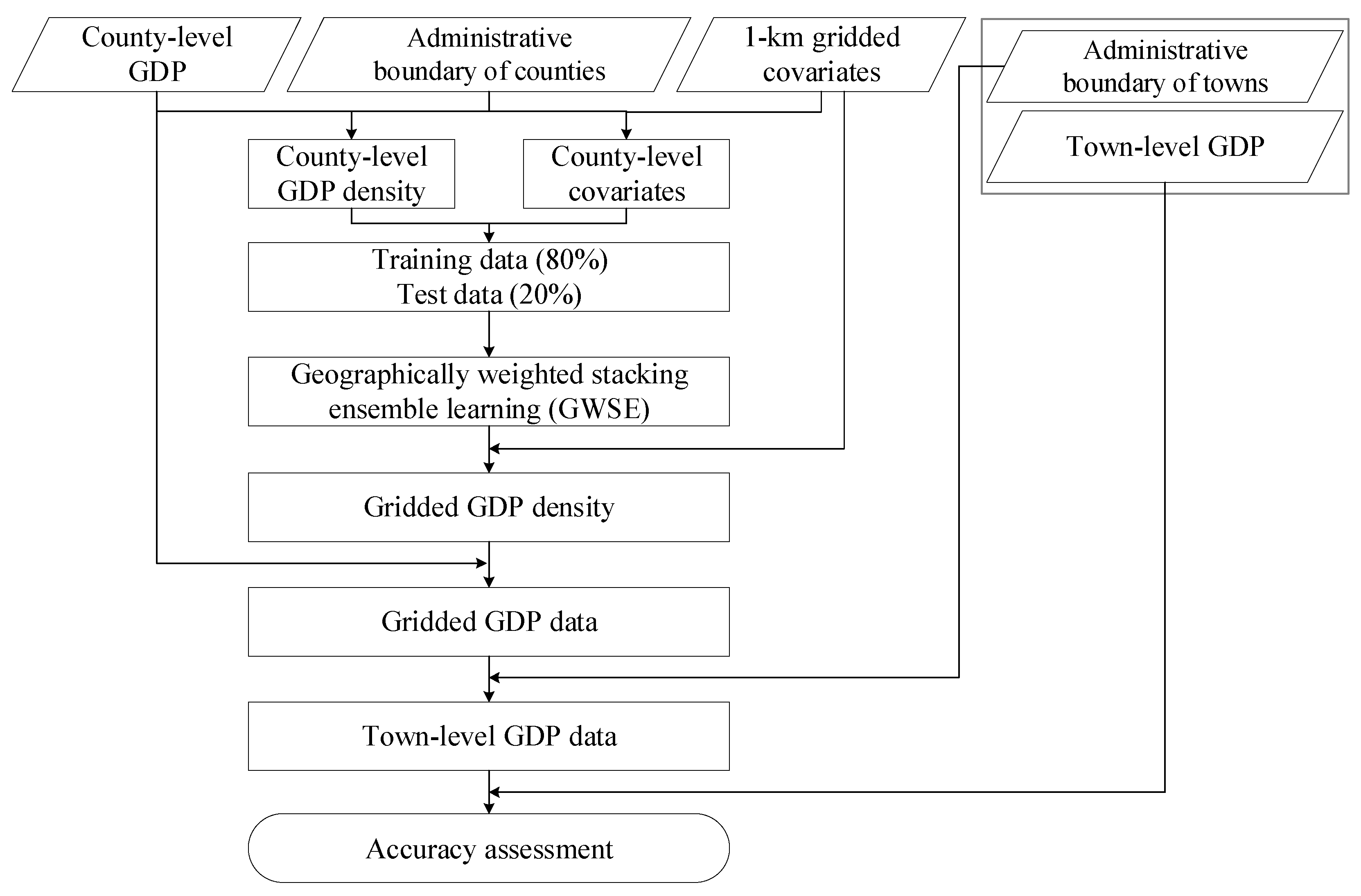
3.1. Procedure of GDP Downscaling

Figure 3 illustrates the procedure of GDP downscaling, which consisted of the following four processes.
(1)
The county-level GDP data in Figure 1 and 1 km covariates in Table 1 were preprocessed. The Albers equal-area conic projection was adopted as the coordinate system of the GDP data and covariates. The county-level covariates were also calculated using the mean of covariates within each county and were combined with county-level GDP data for subsequent training.
(2)
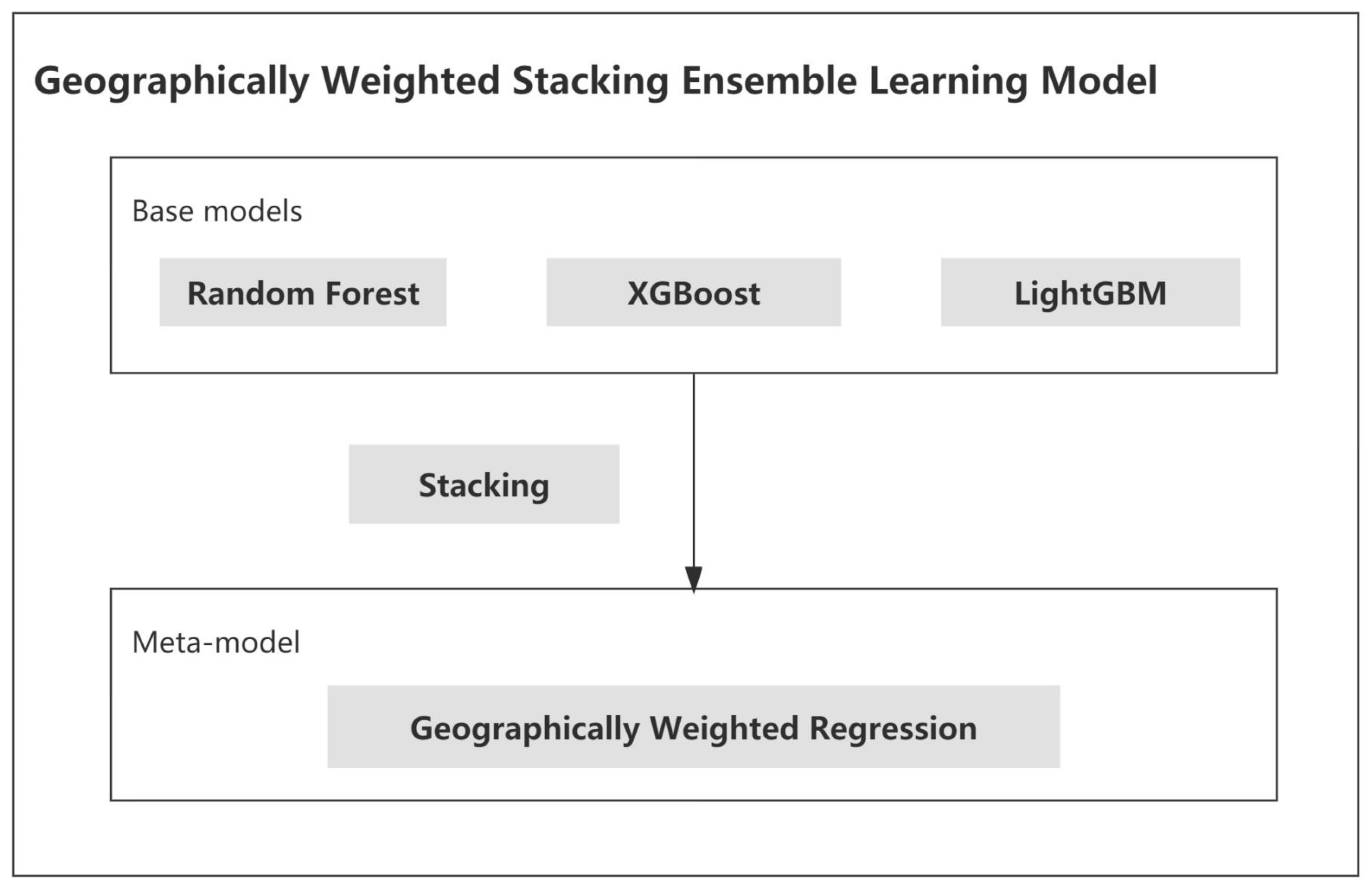
GWSE was built and trained to estimate gridded GDP density. Random forest, XGBoost, and LightGBM were employed as base models, and the longitude and latitude were considered as covariates in the three models to account for spatial homogeneity. To consider spatial heterogeneity, GWSE replaced linear regression with GWR to locally fuse the predictions of the three base models in stacking ensemble learning. As each GDP sector has different spatial distribution and related covariates [10,23,27,28,42], three GWSE models were trained for each GDP sector to estimate the gridded GDP density of each GDP sector. The county-level GDP data and county-level covariates were divided into training data and test data. Training data accounted for 80% of all county-level data in training GWSE for each GDP sector. The best-trained GWSE was selected for each GDP sector after 10 iterations.
(3)
Gridded GDP data was predicted using trained GWSE models. According to previous GDP downscaling studies [2,9,10,23,24], the trained GDP downscaling models on administrative-level data were directly used to estimate the gridded GDP data. Using 1 km gridded covariates as inputs, each trained GWSE model on county-level data was employed to forecast the 1 km gridded GDP density of each GDP sector. The predicted gridded GDP density was adjusted to generate gridded GDP data for each sector, and the sum of the three adjusted gridded GDP data was computed as the total gridded GDP data.
(4)
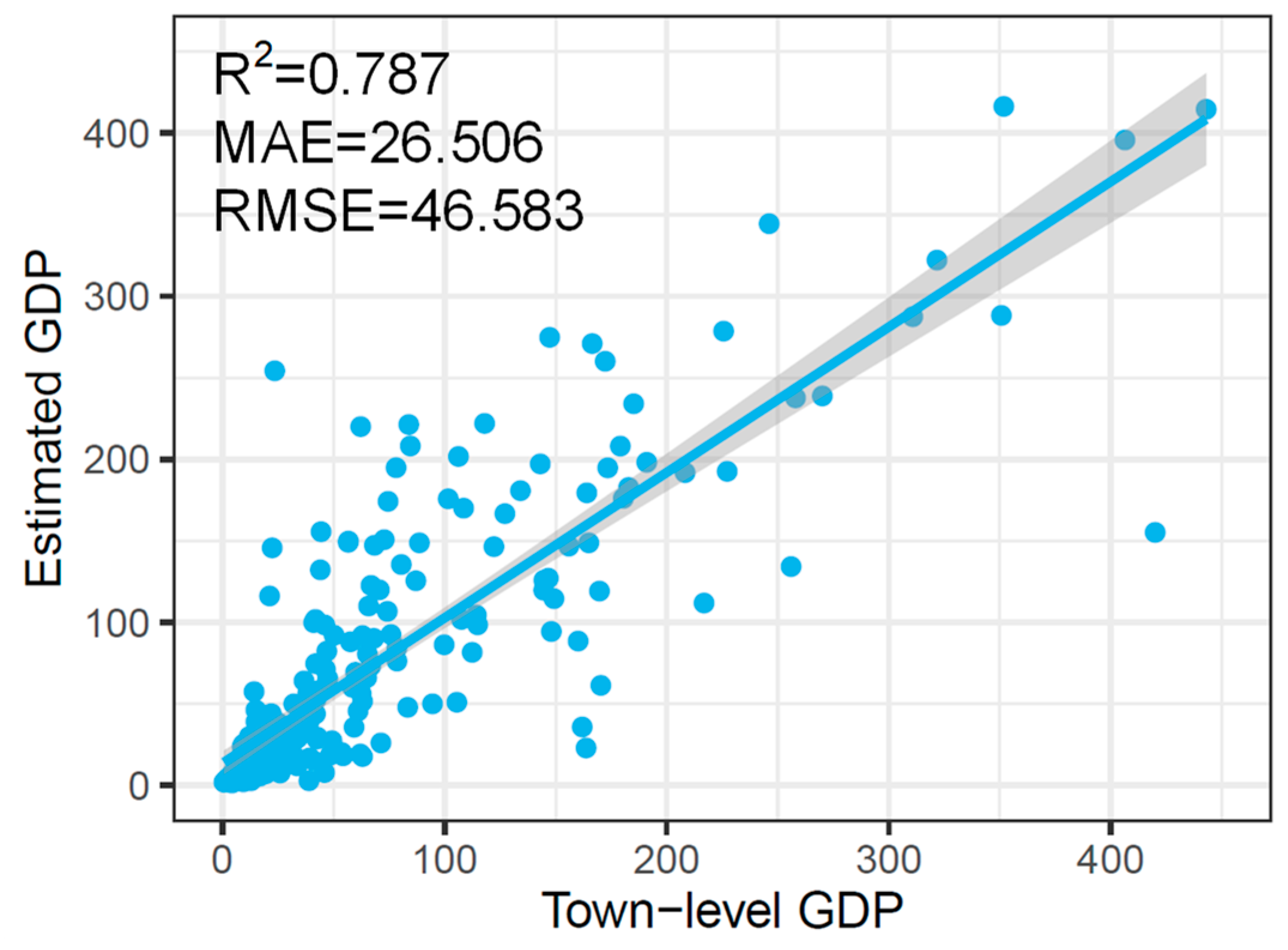
The accuracy of the gridded GDP data was evaluated. Statistical town-level GDP data from the yearbook were adopted as ground truth data to evaluate the corresponding town-level GDP data aggregated from the estimated gridded GDP data to further evaluate the performance of GWSE.

3.2. Preparing GDP and Auxiliary Data
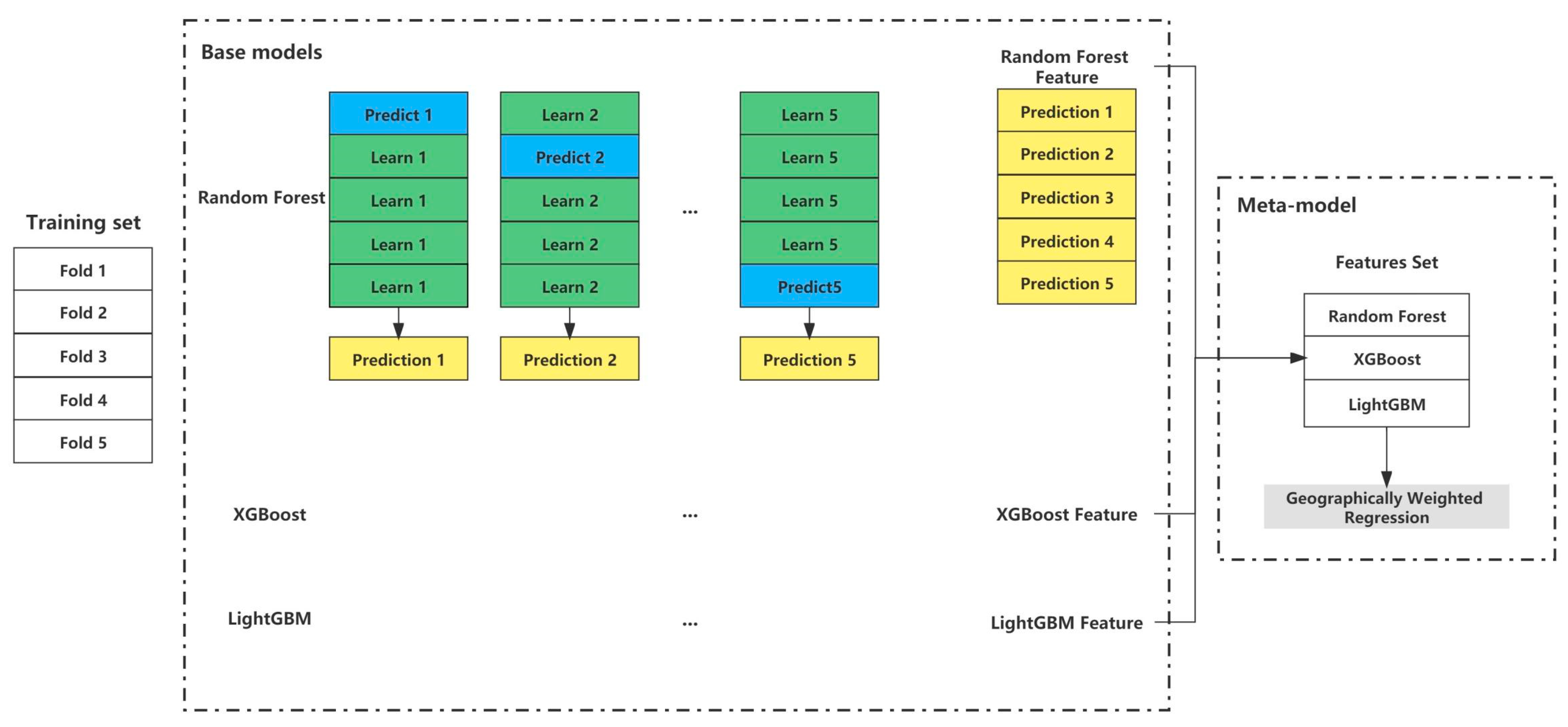
The county-level GDP density was calculated by dividing the GDP in a county by the area of the corresponding county for each GDP sector. The logarithm of GDP density was used as the dependent variable in GWSE training. The county-level covariates were aggregated by the Zonal Statistics tool in ArcGIS from 1 km gridded covariates to spatially align with the county-level GDP data and were employed as independent variables in GWSE training.

3.3. Building GWSE

Ensemble learning combines the results of different algorithms, and it can obtain better results than those obtained from any individual algorithm [29]. Blending and stacking usually combine different types of algorithms. Stacking theoretically outperforms blending as it has a robust training mechanism [32]. Therefore, this study focused on stacking ensemble learning. Ensemble learning is usually made up of base models and a metamodel. Base models are regarded as the individual algorithm while the metamodel aims to fuse the predictions of base models. Random forest is a typical bagging-like ensemble learning approach, and it fuses the results of several decision-tree algorithms of the same type [10]. XGBoost [43] and LightGBM [44] are gradient-boosting ensemble learning methods, and they fuse the results of the same type of decision trees as well. Thus, random forest, XGBoost, and LightGBM were employed as base models. Linear regression is often used as the metamodel to fuse the predictions of the base models. GWR has been theoretically proven to perform better than linear regression in dealing with geographical variables as it considers geographical properties [37] Therefore, the proposed GWSE aims to locally fuse the predictions of the three base models of random forest, XGBoost, and LightGBM. Figure 4 shows the structure of the proposed GWSE. During the fitting process of GWSE, the three base models were first fitted using county-level data. Then, the three county-level predictions of the base models were employed as independent variables and the county-level GDP data as and the dependent variable to fit GWR and linear regression in stacking ensemble learning.

3.3.1. Base Models

Random forest is a combination of the same type of decision trees so that each tree depends on the values of a random vector sampled independently and with the same distribution for all trees in the forest. As the number of trees in a forest increases, the generalization error converges asymptotically to a limit [29].
XGBoost is a scalable and effective use of Friedman’s gradient boosting technology. A tree learning algorithm and an effective linear model solver are included [43].
LightGBM is a gradient-boosting framework that uses decision trees and is designed to be distributed and efficient [44]. Two innovative strategies are included in the LightGBM algorithm, namely, gradient-based one-side sampling and exclusive feature bundling.

3.3.2. Meta Model

Geographically weighted regression (GWR) is a spatial analysis tool [37]. It mainly intends to indicate where nonstationarity is taking place in space, allowing the relationships between the independent and dependent variables to vary by locality. GWR is a modification of the typical linear regression. The basic form of GWR is as follows:
y i = β i 0 + k = 1 m β i k x i k + ϵ i
where y i is the dependent variable at location i; x i k is the kth independent variable at location i; m 1 , 2 , 3 is the number of independent variables and the outputs of the three base models are used as independent variables in this study; β i 0 is the intercept parameter at location i; β i k is the local regression coefficient for the kth independent variable at location i; and ϵ i is the random error at location i.
We used GWmodelS (V1.0.3) software developed by Lu et al. [45] to realize the GWR process of the proposed GWSE for bandwidth selection, coefficient estimation, and prediction.

3.3.3. Stacking

A metamodel is trained in stacking ensembles using CV on the base models’ out-of-fold predictions. Figure 5 illustrates the specific learning process of stacking ensemble learning. In this study, a 5-fold CV was adopted to divide the training set into two parts. Predictions were made with the final fold after fitting each base model using four folds. Each of the 5 folds went through the process again. Then, the metamodel (i.e., GWR) was fitted using the predictions from all base models.

3.4. GDP Downscaling

After the training of GWSE for each GDP sector, the 1 km gridded GDP density of each sector can be estimated as follows:
g k j = e f θ ( x j )
where f θ ( x j ) is the estimated logarithm of GDP density for grid j , x j is the covariates for grid j , and k 1 , 2 , 3 is the index of GDP sectors. The estimated logarithm of GDP density was obtained by the trained GWSE for each GDP sector. GWSE first input the 1 km gridded covariates to the three trained base models, and the fitted GWR then carried out their predictions to estimate the gridded GDP density. Note that each county had individual GWR coefficients for the three predictions of the base models, whereas there was no GWR coefficient for each grid. Thus, referring to previous GDP downscaling studies [2,9,10,23,24], the GWR coefficient of a county was employed as the GWR coefficient of all grids within the county.
To maintain GDP coherency within each county, the gridded GDP density of each sector was adjusted by multiplying the ratio between the actual GDP and the sum of estimated GDP grids within a county as follows:
A G k i = g k i A G k i j i g k j
where A G k i is the actual GDP within county i for sector k .
The total GDP for grid j can be computed as follows:
A G j = k = 1 3 A G k j

3.5. Accuracy Assessment Metrics

In order to evaluate the effectiveness of the proposed GWSE in predicting gridded GDP data, actual town-level GDP data were adopted to compare with the corresponding town-level GDP data aggregated from the estimated 1 km gridded GDP data. Three metrics—mean absolute error (MAE), root mean square error (RMSE), and the coefficient of determination (R2)—were adopted. Their formulas are as follows:
M A E = 1 M i = 1 M A G i A G ˜ i
R M S E = 1 M i = 1 M A G i A G ˜ i 2
R 2 = 1 i = 1 M A G i A G ˜ i 2 i = 1 M A G i A G ¯ 2
where A G i is the actual GDP for town i , A G ˜ i is the estimated GDP for town i , A G ¯ is the mean of actual GDP for all towns, and M is the number of towns.

4. Results

4.1. Model Performance and Comparison

Random forest, XGBoost, and LightGBM were adopted as not only the base models in stacking but also comparison algorithms. The common metamodel of linear regression in stacking ensemble learning was also compared with the proposed GWSE. Three metrics—R2, MAE, and RMSE—were used to evaluate the performance of the five methods for each GDP sector on test data, as shown in Table 2. Higher R2 and lower MAE and RMSE indicated better performance. The three metrics showed that the five methods performed the best for the tertiary sector, then for the secondary sector, and the worst for the primary sector. The three typical machine learning algorithms of random forest, XGBoost, and LightGBM had comparable performance for each GDP sector because they had almost the same R2, as shown in Table 2. The two stacking ensemble learning approaches performed better than any of the base models for each GDP sector. Specifically, the average R2 of the two stacking ensemble learning approaches was 0.035, 0.011, and 0.010 higher than that of the three base models for the primary, secondary, and tertiary sectors, respectively. The proposed GWSE performed the best in the three GDP sectors according to the three metrics in Table 2, which demonstrated the effectiveness of the proposed GWSE. Hence, the trained GWSE models were adopted to generate the gridded GDP data in the case study area of mainland China for the year of 2020.

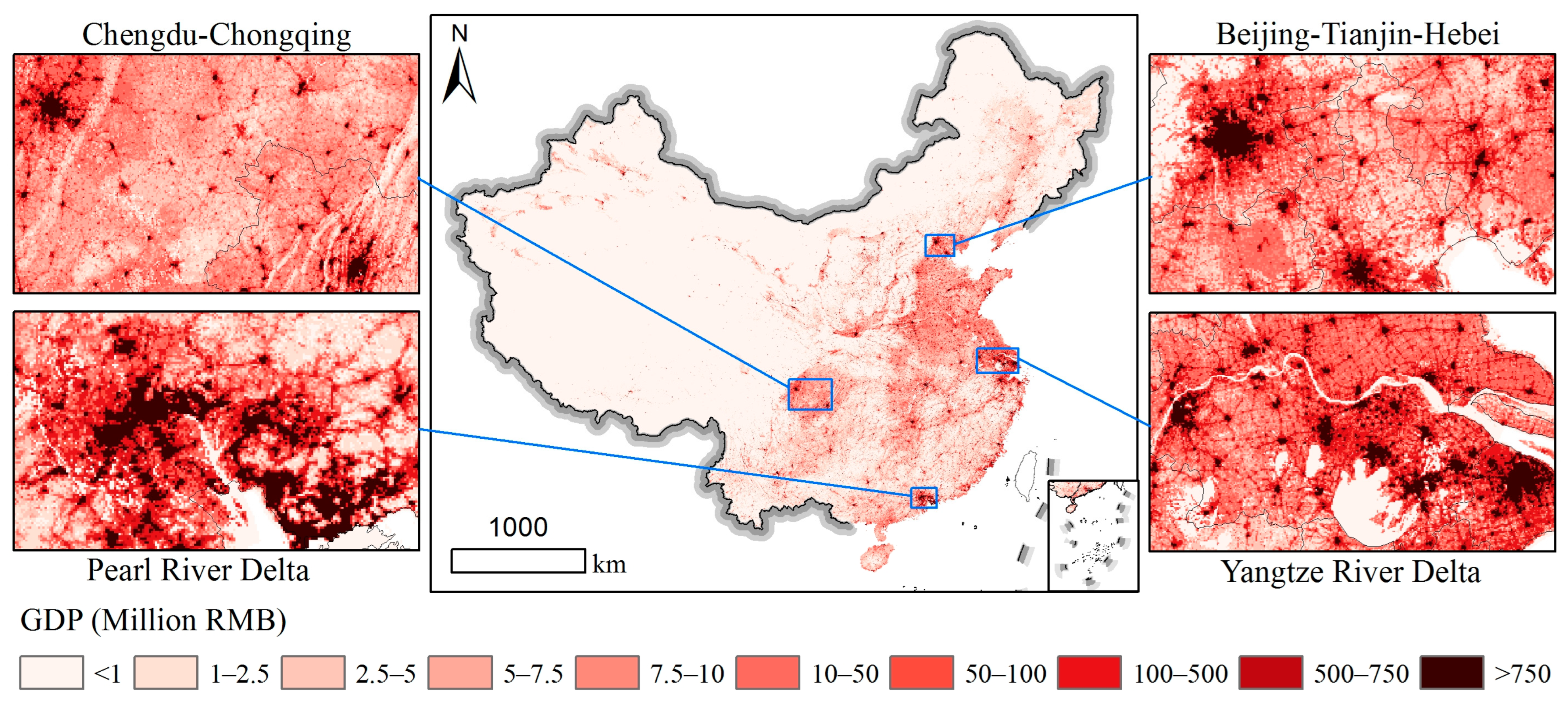
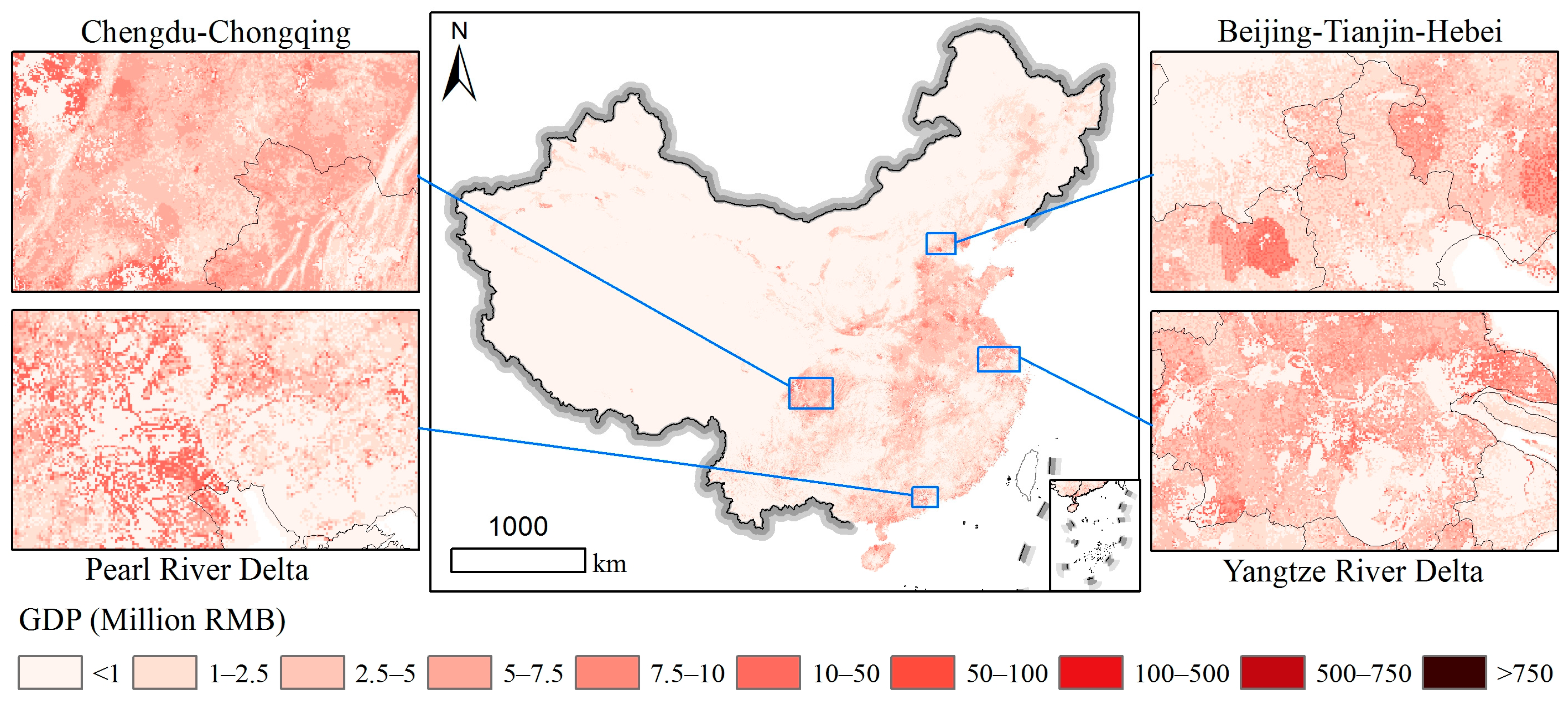
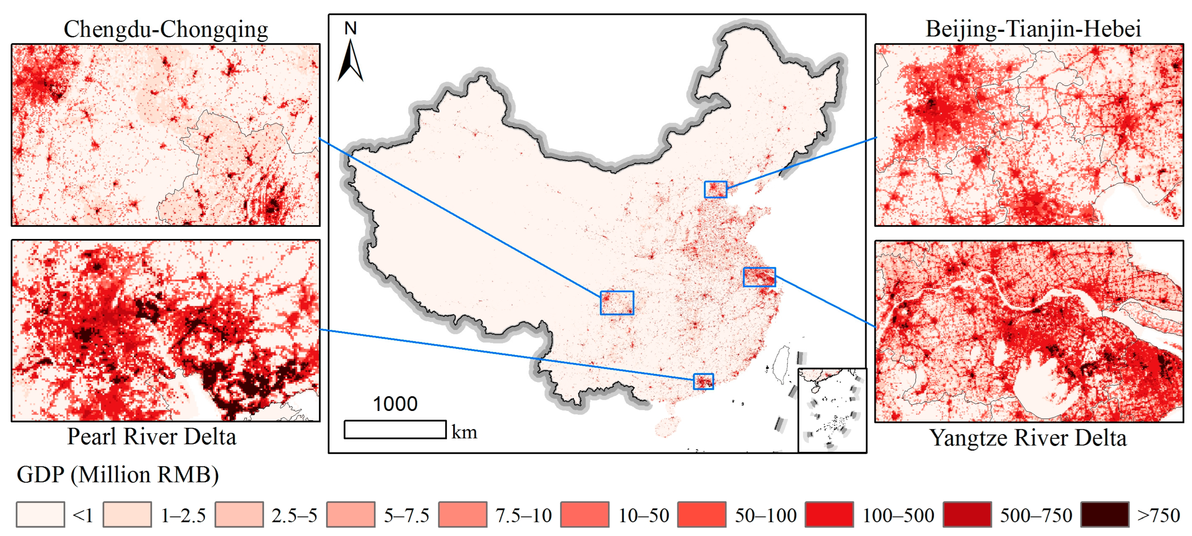
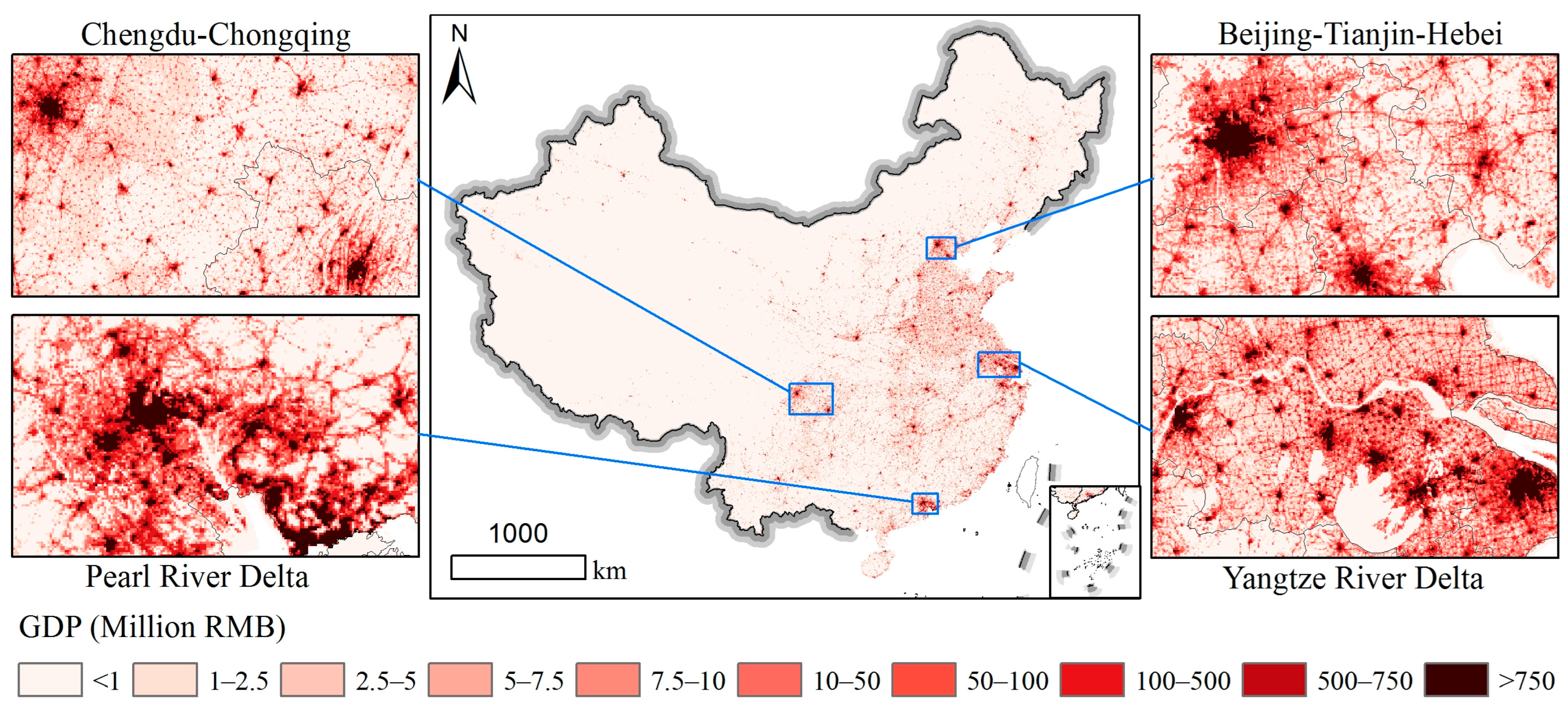
4.2. Gridded GDP Maps

Figure 6 shows the 1 km gridded total GDP map of China. It indicates that relatively high-value GDP grids were dominantly distributed in the Huanghuaihai Plain, Sichuan Basin, the eastern coastal region, and the capital cities of provinces. The GDP spatial distribution was further examined using four representative zoomed-in regions: Chengdu-Chongqing, Beijing–Tianjin–Hebei, Pearl River Delta, and Yangtze River Delta. These are China’s four biggest urban agglomeration regions. The city centers of Beijing, Shanghai, Guangzhou, and Shenzhen exhibited more high-value GDP grids (over 750 million RMB) than other city centers. The spatial distribution of the gridded total GDP data was logically consistent with the fundamental knowledge of GDP in mainland China, suggesting the validity of the proposed GWSE.

4.2.1. Gridded GDP Map of China for the Primary Sector

Figure 7 displays the 1 km gridded GDP map for the primary sector in China. It shows that the gridded GDP for the primary sector was distributed throughout China and its distribution was similar to that of the land cover of crops. It makes sense that the primary sector was mainly related to agricultural activities. Meanwhile, it is reasonable that there were more low-value (less than five million RMB) GDP grids in city centers and more high-value GDP grids in rural areas in the four zoomed-in regions. However, most GDP grids for the primary sector had relatively low value than those in the gridded total GDP map in Figure 6.

4.2.2. Gridded GDP Map of China for the Secondary Sector

Figure 8 shows the 1 km gridded GDP map for the secondary sector in China. Its spatial distribution was mainly scattered around big cities. The relatively high-value GDP grids for the secondary sector were clustered in urban suburbs. The four zoomed-in regions indicated that the Pearl River Delta had the most high-value GDP grids, followed by the Yangtze River Delta and the Beijing–Tianjin–Hebei region, and the Chengdu–Chongqing region had the least high-value GDP grids in visual examination for the gridded GDP of the secondary sector. Even so, the Yangtze River Delta presented a more even distribution than the other three zoomed-in regions, indicating more balanced development of the secondary sector of GDP there.

4.2.3. Gridded GDP Map of China for the Tertiary Sector

Figure 9 presents the 1 km gridded GDP map of China for the tertiary sector. The overview showed they were also scattered around big cities and the relatively high-value GDP grids for the tertiary sector were clustered in urban centers. When focusing on the four zoomed-in regions, high-value GDP grids were mainly located in eight city centers (i.e., Chengdu, Chongqing, Beijing, Tianjin, Guangzhou, Shenzhen, Nanjing, and Shanghai). It is reasonable that the city center had a more clustered population and service activities relevant to the tertiary sector of GDP.

4.3. Accuracy Assessment

There were 284 town-level total GDP data collected for the accuracy assessment of the gridded total GDP data at a fine scale. As can be seen from Figure 10, R2 reached a high value (0.787), indicating the 1 km gridded GDP data had a high accuracy at the town-level scale. The MAE and RMSE of the gridded total GDP result within the 284 towns were 2.65 billion and 4.66 billion RMB, respectively, implying a relatively low error of the estimated gridded GDP. This further proves the effectiveness of the proposed GWSE and its value for generating gridded GDP data in other regions. Although the generated gridded total GDP result evaluated by town-level GDP data had a relatively high accuracy, there was a significant distinction. As shown in Figure 10, most towns with less than 5 billion RMB had relatively lower errors as they were closely distributed along the fitted regression line. On the contrary, some towns with over 5 billion RMB were scattered on both sides of the fitted regression line. This means that the estimated GDP result may have relatively larger error in high GDP grids and relatively smaller error in low GDP grids.

5. Discussion

5.1. Difference in Performance of GDP Sectors

As each GDP sector had different distributions and related covariates, separate methods were built and trained with different covariates for each GDP sector. Table 2 shows that the five methods performed the best in the tertiary sector and the worst in the primary sector and that the secondary and tertiary sectors had comparable performance. Specifically, the average R2 values of the primary, secondary, and tertiary sectors were 0.8718, 0.969, and 0.9694; the average MAE was 0.788, 0.2718, and 0.2638; and the average RMSE was 1.0834, 0.3674, and 0.3626. It is likely that the accuracy of the covariates relevant to the primary sector was lower than those of the secondary and tertiary sectors. For instance, six land cover classes were used for the primary sector while only one land cover class was used for the other two sectors, and the limited accuracy of the six land cover classes would have impacted the performance.
Comparing the four zoomed-in regions in Figure 7, Figure 8 and Figure 9, there were distinct spatial distribution differences among the three sectors. The primary sector had more low-value GDP grids and they were mainly located in rural areas. The secondary sector had more high-value GDP grids, and they were dominantly distributed in urban suburbs. The tertiary sector had more high-value GDP grids in urban centers. The tertiary sector had relatively more high-value grids than the sector in the four zoomed-in regions. The spatial distribution difference of the three gridded GDP data was consistent with the reality of GDP distribution.

5.2. Scale Uncertainty in Estimating Gridded GDP Density

Most current GDP downscaling studies use administrative-level GDP data and covariates to fit the GDP downscaling methods because the real gridded GDP data are hard to collect [2,9,10,23,24]. Fitted GDP downscaling methods using administrative-level GDP data are often adopted to estimate gridded GDP data with gridded covariates as inputs. Therefore, similar to previous GDP downscaling studies, there was a scale uncertainty when the county-level trained GWSE was directly used to estimate the gridded GDP density in this study. Although the estimated gridded GDP data in mainland China demonstrated the effectiveness of the proposed GWSE, the scale uncertainty when downscaling GDP remains.

5.3. Advantages and Disadvantages

Compared to previous GDP downscaling studies, the proposed GWSE had several characteristics and advantages in terms of the estimated gridded GDP data. First, it performed better than the three base algorithms according to the metrics in Table 2, which implied that the advantages of each base algorithm were encapsulated in the proposed GWSE. Second, GWSE took the geographical properties into account and thus generated gridded GDP data with higher accuracy compared to traditional stacking ensemble learning because GWSE replaced linear regression with GWR to fuse the predictions of base models. Third, the proposed GWSE could consider the simple relationship between GDP data and covariates as well as the nonlinear complex relationship in GDP downscaling.
This research has some disadvantages as well. High-quality covariates are critical for generating highly accurate gridded GDP data. The quality of a few covariates used in this study was limited, and this influenced the gridded GDP data. For instance, the used POIs as points only provided the quantity information instead of the area of each POI, which is more valuable than points for generating gridded GDP. Meanwhile, only three widely used algorithms were employed here as base models and the learning ability of the proposed GWSE was therefore limited by the skills of those base models. Further, GWSE is similar to previous GDP downscaling methods, and it has the scale uncertainty in estimating gridded GDP density. When fitting GWSE in the GWR process, there is no multicollinearity problem. However, the multicollinearity problem is an intrinsic problem of stacking ensemble learning in fusing the predictions of base models. GWSE is no exception, and it may encounter the multicollinearity problem when using different base models in other GDP downscaling applications.

5.4. Future Work

Further improvements to this research can be made in the future. High-quality covariates can be further collected, which may improve the results of the trained GWSE and the subsequent gridded GDP data. Meanwhile, there were a total of 19 covariates for generating gridded GDP data in this study, and other covariates relevant to GDP can be added to the proposed GWSE in future studies. In this case study, only three base models were used in GWSE to downscale GDP data. Various combinations of other base models can be investigated to examine the performance improvement of GWSE in future. The scale uncertainty of GWSE in estimating gridded GDP data is worth addressing by some potential techniques, such as the scale transformation methods [46]. Additionally, GWSE may encounter the multicollinearity problem and the penalized GWR can be used to address this problem [47].

6. Conclusions

Gridded gross domestic product (GDP) data are highly desired in many applications. In recent years, machine learning approaches have become robust tools in generating gridded GDP data. This paper presents a novel GDP downscaling approach by considering geographical properties of variables. Three algorithms were used as base models, and geographically weighted regression was adopted to locally fuse the predictions of the base models in stacking ensemble learning. The case study was conducted in mainland China to demonstrate the effectiveness and ability of the proposed approach. The results indicated that the proposed GDP downscaling approach outperformed the four existing machine learning algorithms. Meanwhile, it had good predictive power on county-level GDP data with R2 of 0.894, 0.976, and 0.976 for the primary, secondary, and tertiary sectors, respectively. Furthermore, the estimated 1 km gridded GDP data had a high accuracy (R2 = 0.787) evaluated by town-level GDP data. Additionally, the generated 1 km gridded GDP data of China from 2020 can be valuable for other applications in China.

Author Contributions

Conceptualization, Yuehong Chen and Qiang Ma; methodology, Zekun Xu and Yuehong Chen; formal analysis, Zekun Xu, Yu Wang and Guihou Sun; writing—original draft preparation, Yuehong Chen and Zekun Xu; writing—review and editing, Yu Wang, Qiang Ma and Xiaoxiang Zhang. All authors have read and agreed to the published version of the manuscript.

Funding

This research was funded in part by the Key Research and Development Program of Guangxi Province [No. 2019AB20003], in part by the National Key Research and Development Program of China [No. 2019YFC1510601], and in part by the National Natural Science Foundation of China [No. 42071315].

Institutional Review Board Statement

Not applicable.

Informed Consent Statement

Not applicable.

Data Availability Statement

All data relevant to the study are presented in the article. For further inquiries regarding the reuse of data, please contact the corresponding authors.

Conflicts of Interest

The authors declare no conflict of interest.

References

  1. Geiger, T. Continuous national gross domestic product (gdp) time series for 195 countries: Past observations (1850–2005) harmonized with future projections according to the shared socio-economic pathways (2006–2100). Earth Syst. Sci. Data 2018, 10, 847–856. [Google Scholar] [CrossRef] [Green Version]
  2. Huang, Z.; Li, S.; Gao, F.; Wang, F.; Lin, J.; Tan, Z. Evaluating the performance of lbsm data to estimate the gross domestic product of china at multiple scales: A comparison with npp-viirs nighttime light data. J. Clean. Prod. 2021, 328, 129558. [Google Scholar] [CrossRef]
  3. Kummu, M.; Taka, M.; Guillaume, J.H.A. Gridded global datasets for gross domestic product and human development index over 1990–2015. Sci. Data 2018, 5, 180004. [Google Scholar] [CrossRef] [Green Version]
  4. Nadim, F.; Kjekstad, O.; Peduzzi, P.; Herold, C.; Jaedicke, C. Global landslide and avalanche hotspots. Landslides 2006, 3, 159–173. [Google Scholar] [CrossRef]
  5. Sun, J.; Di, L.; Sun, Z.; Wang, J.; Wu, Y. Estimation of gdp using deep learning with npp-viirs imagery and land cover data at the county level in conus. IEEE J. Sel. Top. Appl. Earth Obs. Remote Sens. 2020, 13, 1400–1415. [Google Scholar] [CrossRef]
  6. Sutton, P.C.; Costanza, R. Global estimates of market and non-market values derived from nighttime satellite imagery, land cover, and ecosystem service valuation. Ecol. Econ. 2002, 41, 509–527. [Google Scholar] [CrossRef]
  7. Yao, J.; Zhang, X.; Luo, W.; Liu, C.; Ren, L. Applications of stacking/blending ensemble learning approaches for evaluating flash flood susceptibility. Int. J. Appl. Earth Obs. Geoinf. 2022, 112, 102932. [Google Scholar] [CrossRef]
  8. Yi, J.; Du, Y.; Liang, F.; Tu, W.; Qi, W.; Ge, Y. Mapping human’s digital footprints on the tibetan plateau from multi-source geospatial big data. Sci. Total Environ. 2019, 711, 134540. [Google Scholar] [CrossRef]
  9. Zhao, N.; Liu, Y.; Cao, G.; Samson, E.L.; Zhang, J. Forecasting china’s gdp at the pixel level using nighttime lights time series and population images. GIScience Remote Sens. 2017, 54, 407–425. [Google Scholar] [CrossRef]
  10. Chen, Q.; Ye, T.; Zhao, N.; Ding, M.; Ouyang, Z.; Jia, P.; Yue, W.; Yang, X. Mapping china’s regional economic activity by integrating points-of-interest and remote sensing data with random forest. Environ. Plan. B Urban Anal. City Sci. 2020, 48, 1876–1894. [Google Scholar] [CrossRef]
  11. Wang, X.; Sutton, P.C.; Qi, B. Global mapping of gdp at 1 km2 using viirs nighttime satellite imagery. ISPRS Int. J. Geo-Inf. 2019, 8, 580. [Google Scholar] [CrossRef] [Green Version]
  12. Lloyd, C.T.; Sorichetta, A.; Tatem, A. High resolution global gridded data for use in population studies. Sci. Data 2017, 4, 170001. [Google Scholar] [CrossRef] [PubMed] [Green Version]
  13. Doll, C.N.; Muller, J.-P.; Elvidge, C.D. Night-time imagery as a tool for global mapping of socioeconomic parameters and greenhouse gas emissions. AMBIO J. Hum. Environ. 2000, 29, 157–162. [Google Scholar] [CrossRef]
  14. Elvidge, C.D.; Baugh, K.E.; Kihn, E.A.; Kroehl, H.W.; Davis, E.R.; Davis, C.W. Relation between satellite observed visible-near infrared emissions, population, economic activity and electric power consumption. Int. J. Remote Sens. 1997, 18, 1373–1379. [Google Scholar] [CrossRef]
  15. Zhang, R.; Chen, Y.; Zhang, X.; Ma, Q.; Ren, L. Mapping homogeneous regions for flash floods using machine learning: A case study in jiangxi province, china. Int. J. Appl. Earth Obs. Geoinf. 2022, 108, 102717. [Google Scholar] [CrossRef]
  16. Liu, Y.; Liu, X.; Gao, S.; Gong, L.; Kang, C.; Zhi, Y.; Chi, G.; Shi, L. Social sensing: A new approach to understanding our socioeconomic environments. Ann. Assoc. Am. Geogr. 2015, 105, 512–530. [Google Scholar] [CrossRef]
  17. Chen, Y.; Shi, K.; Ge, Y.; Zhou, Y.n. Spatiotemporal remote sensing image fusion using multiscale two-stream convolutional neural networks. IEEE Trans. Geosci. Remote Sens. 2022, 60, 1–12. [Google Scholar] [CrossRef]
  18. Chen, Y.; Li, Y.; Wu, G.; Zhang, F.; Zhu, K.; Xia, Z.; Chen, Y. Exploring spatiotemporal accessibility of urban fire services using real-time travel time. Int. J. Environ. Res. Public Health 2021, 18, 4200. [Google Scholar] [CrossRef]
  19. Chen, Y.; Ge, Y.; Chen, Y.; Jin, Y.; An, R. Subpixel land cover mapping using multiscale spatial dependence. IEEE Trans. Geosci. Remote Sens. 2018, 56, 5097–5106. [Google Scholar] [CrossRef]
  20. Chen, Y.; Ge, Y.; Heuvelink, G.B.M.; An, R.; Chen, Y. Object-based superresolution land cover mapping from remotely sensed imagery. IEEE Trans. Geosci. Remote Sens. 2018, 56, 328–340. [Google Scholar] [CrossRef]
  21. Chen, Y.; Ge, Y.; An, R.; Chen, Y. Super-resolution mapping of impervious surfaces from remotely sensed imagery with points-of-interest. Remote Sens. 2018, 10, 242. [Google Scholar] [CrossRef] [Green Version]
  22. Chen, Y.; Zhou, Y.n.; Ge, Y.; An, R.; Chen, Y. Enhancing land cover mapping through integration of pixel-based and object-based classifications from remotely sensed imagery. Remote Sens. 2018, 10, 77. [Google Scholar] [CrossRef] [Green Version]
  23. Chen, Q.; Hou, X.; Zhang, X.; Ma, C. Improved gdp spatialization approach by combining land-use data and night-time light data: A case study in china’s continental coastal area. Int. J. Remote Sens. 2016, 37, 4610–4622. [Google Scholar] [CrossRef] [Green Version]
  24. Murakami, D.; Yamagata, Y. Estimation of gridded population and gdp scenarios with spatially explicit statistical downscaling. Sustainability 2019, 11, 2106. [Google Scholar] [CrossRef] [Green Version]
  25. Zhao, M.; Cheng, W.; Zhou, C.; Li, M.; Wang, N.; Liu, Q. Gdp spatialization and economic differences in south china based on npp-viirs nighttime light imagery. Remote Sens. 2017, 9, 673. [Google Scholar] [CrossRef] [Green Version]
  26. Liang, H.; Guo, Z.; Wu, J.; Chen, Z. Gdp spatialization in ningbo city based on npp/viirs night-time light and auxiliary data using random forest regression. Adv. Space Res. 2020, 65, 481–493. [Google Scholar] [CrossRef]
  27. Chen, Y.; Wu, G.; Ge, Y.; Xu, Z. Mapping gridded gross domestic product distribution of china using deep learning with multiple geospatial big data. IEEE J. Sel. Top. Appl. Earth Observ. Remote Sens 2022, 15, 1791–1802. [Google Scholar] [CrossRef]
  28. Ustaoglu, E.; Bovkır, R.; Aydınoglu, A.C. Spatial distribution of gdp based on integrated nps-viirs nighttime light and modis evi data: A case study of turkey. Environ. Dev. Sustain. 2021, 23, 10309–10343. [Google Scholar] [CrossRef]
  29. Dong, X.; Yu, Z.; Cao, W.; Shi, Y.; Ma, Q. A survey on ensemble learning. Front. Comput. Sci. 2020, 14, 241–258. [Google Scholar] [CrossRef]
  30. Wu, T.; Zhang, W.; Jiao, X.; Guo, W.; Alhaj Hamoud, Y. Evaluation of stacking and blending ensemble learning methods for estimating daily reference evapotranspiration. Comput. Electron. Agric. 2021, 184, 106039. [Google Scholar] [CrossRef]
  31. Cheng, J.; Sun, J.; Yao, K.; Xu, M.; Wang, S.; Fu, L. Hyperspectral technique combined with stacking and blending ensemble learning method for detection of cadmium content in oilseed rape leaves. J. Sci. Food Agric. 2022, 103, 2690–2699. [Google Scholar] [CrossRef] [PubMed]
  32. Džeroski, S.; Ženko, B. Is combining classifiers with stacking better than selecting the best one? Mach. Learn. 2004, 54, 255–273. [Google Scholar] [CrossRef] [Green Version]
  33. Oshan, T.M.; Li, Z.; Kang, W.; Wolf, L.J.; Fotheringham, A.S. Mgwr: A python implementation of multiscale geographically weighted regression for investigating process spatial heterogeneity and scale. ISPRS Int. J. Geo-Inf. 2019, 8, 269. [Google Scholar] [CrossRef] [Green Version]
  34. Song, Y. Geographically optimal similarity. Math. Geosci. 2022, 1–26. [Google Scholar] [CrossRef]
  35. Georganos, S.; Grippa, T.; Niang Gadiaga, A.; Linard, C.; Lennert, M.; Vanhuysse, S.; Mboga, N.; Wolff, E.; Kalogirou, S. Geographical random forests: A spatial extension of the random forest algorithm to address spatial heterogeneity in remote sensing and population modelling. Geocarto Int. 2021, 36, 121–136. [Google Scholar] [CrossRef] [Green Version]
  36. Chen, Y.; Wu, G.; Chen, Y.; Xia, Z. Spatial location optimization of fire stations with traffic status and urban functional areas. Appl. Spat. Anal. Policy 2023, 1–18. [Google Scholar] [CrossRef]
  37. Fotheringham, A.; Brunsdon, C.; Charlton, M. Geographically Weighted Regression: The Analysis of Spatially Varying Relationships; Wiley: Chichester, UK; Hoboken, NJ, USA, 2002. [Google Scholar]
  38. Chen, Y.; Ruojing, Z.; Ge, Y.; Yan, J.; Zelong, X. Downscaling census data for gridded population mapping with geographically weighted area-to-point regression kriging. IEEE Access 2019, 7, 149132–149141. [Google Scholar] [CrossRef]
  39. Goodchild, M.F. The validity and usefulness of laws in geographic information science and geography. Ann. Assoc. Am. Geogr. 2004, 94, 300–303. [Google Scholar] [CrossRef] [Green Version]
  40. Elvidge, C.D.; Zhizhin, M.; Ghosh, T.; Hsu, F.-C.; Taneja, J. Annual time series of global viirs nighttime lights derived from monthly averages: 2012 to 2019. Remote Sens. 2021, 13, 922. [Google Scholar] [CrossRef]
  41. Karra, K.; Kontgis, C.; Statman-Weil, Z.; Mazzariello, J.C.; Mathis, M.; Brumby, S.P. Global land use/land cover with sentinel 2 and deep learning. In Proceedings of the 2021 IEEE International Geoscience and Remote Sensing Symposium IGARSS, Brussels, Belgium, 11–16 July 2021; pp. 4704–4707. [Google Scholar]
  42. Thomas, T.S.; You, L.; Wood-Sichra, U.; Ru, Y.; Blankespoor, B.; Kalvelagen, E.M.F. Generating Gridded Agricultural Gross Domestic Product for Brazil: A Comparison of Methodologies; The World Bank: Washington, DC, USA, 2019. [Google Scholar] [CrossRef] [Green Version]
  43. Chen, T.; Guestrin, C. Xgboost: A scalable tree boosting system. In Proceedings of the 22nd Acm Sigkdd International Conference on Knowledge Discovery and Data Mining, San Francisco, CA, USA, 13–17 August 2016; pp. 785–794. [Google Scholar] [CrossRef] [Green Version]
  44. Ke, G.; Meng, Q.; Finley, T.; Wang, T.; Chen, W.; Ma, W.; Ye, Q.; Liu, T.-Y. Lightgbm: A highly efficient gradient boosting decision tree. Adv. Neural Inf. Process. Syst. 2017, 30, 3146–3154. [Google Scholar]
  45. Lu, B.; Hu, Y.; Yang, D.; Liu, Y.; Liao, L.; Yin, Z.; Xia, T.; Dong, Z.; Harris, P.; Brunsdon, C.; et al. Gwmodels: A software for geographically weighted models. SoftwareX 2023, 21, 101291. [Google Scholar] [CrossRef]
  46. Ge, Y.; Jin, Y.; Stein, A.; Chen, Y.; Wang, J.; Wang, J.; Cheng, Q.; Bai, H.; Liu, M.; Atkinson, P.M. Principles and methods of scaling geospatial earth science data. Earth-Sci. Rev. 2019, 197, 102897. [Google Scholar] [CrossRef]
  47. Wheeler, D.C. Diagnostic tools and a remedial method for collinearity in geographically weighted regression. Environ. Plan. A 2007, 39, 2464–2481. [Google Scholar] [CrossRef]
Figure 1. County-level GDP data in mainland China: (a) primary sector, (b) secondary sector, (c) tertiary sector, (d) total GDP.
Ijgi 12 00123 g001
Figure 2. The 1 km gridded covariates of China: (a) NTL, (b) POI density for the secondary sector, (c) POI density for the tertiary sector, (d) land cover, (e) DEM, (f) slope, (g) road density, and (h) Tencent user density.
Ijgi 12 00123 g002
Figure 3. Procedure of GDP downscaling using GWSE.
Ijgi 12 00123 g003
Figure 4. Structure of GWSE.
Ijgi 12 00123 g004
Figure 5. Procedure of stacking ensemble learning.
Ijgi 12 00123 g005
Figure 6. The 1 km gridded total GDP map of China.
Ijgi 12 00123 g006
Figure 7. The 1 km gridded GDP map of China for the primary sector.
Ijgi 12 00123 g007
Figure 8. The 1 km gridded GDP map of China for the secondary sector.
Ijgi 12 00123 g008
Figure 9. The 1 km gridded GDP map of China for the tertiary sector.
Ijgi 12 00123 g009
Figure 10. Accuracy of gridded total GDP data evaluated by town-level GDP data.
Ijgi 12 00123 g010
Table 1. Covariates for the GDP downscaling of China.
Auxiliary Data VariableDescriptionData SourceTimeUse in Sectors
NTLVIIRS night-time light dataVIIRS NTL image (https://eogdata.mines.edu/nighttime_light/annual/v20/, accessed on 1 January 2022.)2020GDP2 and GDP3
POI density for GDP2Number of POIs within each grid related to GDP2AutoNavi Maps (https://amap.com/, accessed on 31 December 2020.)2020GDP2
POI density for GDP3Number of POIs within each grid related to GDP3GDP3
WaterWater and snow/ice proportion.Esri 10-m global land cover data (https://www.arcgis.com/apps/instant/media/index.html?appid=fc92d38533d440078f17678ebc20e8e2, accessed on 27 December 2021.)2020GDP1
TreeTree proportionGDP1
GrassGrass and flooded vegetation proportionGDP1
CropsCrop land proportionGDP1
Scrub/shrubScrub and shrub proportionGDP1
Bare groundBare ground proportionGDP1
Built areaBuilt area proportionGDP2 and GDP3
DEMDigital elevation of each gridALOS World 3D-30 m (AW3D30)
(https://www.eorc.jaxa.jp/ALOS/en/aw3d30/data/index.htm, accessed on 1 July 2022.)
-GDP1
SlopeSlope of each gridGDP1
Road densityRoad length within each gridAutoNavi Maps (https://amap.com/, accessed on 31 December 2020.)2020GDP2 and GDP3
Tencent user densityAverage positioning density of Tencent usersTencent user positioning data
(https://heat.qq.com/, accessed on 12 June 2019.)
2019GDP2 and GDP3
Percentage of GDP1Percentage of the primary sector in total GDPThe 2021 yearbook of China
(https://data.cnki.net/Yearbook/Single/N2022040099, accessed on 13 April 2022.)
2020GDP1
Percentage of GDP2Percentage of the secondary sector in total GDPGDP2
Percentage of GDP3Percentage of the tertiary sector in total GDPGDP3
LongitudeLongitude of the grid centerCentroid of grids-All three sectors
LatitudeLatitude of the grid centerAll three sectors
Table 2. Performance comparison of different methods on test data.
ModelR2MAERMSE
GDP1Random forest0.8570.3670.531
XGBoost0.8511.4041.889
LightGBM0.8651.4761.998
Stacking (LR)0.8920.3450.497
Stacking (GWR)0.8940.3480.502
GDP2Random forest0.9630.2960.402
XGBoost0.9630.2910.394
LightGBM0.9680.2630.367
Stacking (LR)0.9750.2560.345
Stacking (GWR)0.9760.2530.329
GDP3Random forest0.9650.2660.378
XGBoost0.9640.2830.380
LightGBM0.9670.2740.403
Stacking (LR)0.9750.2530.330
Stacking (GWR)0.9760.2430.322
Disclaimer/Publisher’s Note: The statements, opinions and data contained in all publications are solely those of the individual author(s) and contributor(s) and not of MDPI and/or the editor(s). MDPI and/or the editor(s) disclaim responsibility for any injury to people or property resulting from any ideas, methods, instructions or products referred to in the content.

