Does Time Smoothen Space? Implications for Space-Time Representation

Abstract

The continuous nature of space and time is a fundamental tenet of many scientific endeavors. That digital representation imposes granularity is well recognized, but whether it is possible to address space completely remains unanswered. This paper argues Hales’ proof of Kepler’s conjecture on the packing of hard spheres suggests the answer to be “no”, providing examples of why this matters in GIS generally and considering implications for spatio-temporal GIS in particular. It seeks to resolve the dichotomy between continuous and granular space by showing how a continuous space may be emergent over a random graph. However, the projection of this latent space into 3D/4D imposes granularity. Perhaps surprisingly, representing space and time as locally conjugate may be key to addressing a “smooth” spatial continuum. This insight leads to the suggestion of Face Centered Cubic Packing as a space-time topology but also raises further questions for spatio-temporal representation.

1. Introduction

This work started with a seemingly simple hypothesis: “Any and all locations on a map may be uniquely addressed with arbitrary precision”. If true, then errors due to grain may be assumed to tend, at least asymptotically, toward zero at a high enough resolution. If not, addressable space would seem to be fundamentally different from continuous space, with granularity being fundamental, not merely imposed by the data resolution.

The hypothesis will be shown to be false (at least for Euclidean space). This is of theoretical interest but also practical import when small uncertainties carry decisive implications. Section 3 attempts to resolve the apparent dichotomy from a limited set of logical premises. It succeeds in so far as showing how relative position may be fully addressed but fails to achieve the same for absolute position in Euclidean space. The attempt, however, shows the importance of the duality between space and time, leading to the title question: “Does time smoothen space?” i.e., if Euclidean space cannot be completely addressed all at once, perhaps it can be over time?

As such, the paper makes two contributions to the issue of space-time representation. At the theoretical level, it raises the previously overlooked possibility that analytical space is fundamentally incomplete in a scale-independent manner rather than merely spatial data being imprecise at a given scale. At the practical level, it is noted that this incomplete part may be less easily generalized in spatio-temporal analysis, particularly in applications that are inevitably close to the grain, such as immersive spatial query. Face Centered Cubic Packing is then proposed as a novel approach to represent space-time.

1.1. Research Background

1.1.1. Spatial Granularity in Theory

“Granularity is closely related, but not identical, to imprecision. Granularity refers to the existence of clumps or grains in information, in the sense that individual elements in the grain cannot be distinguished or discerned apart”. Duckham et al. [1]

If Euclid’s Elements is the quintessential early text to reference ideas of continuous space, Logistica (by Barlaam of Seminara 1290–1350) was the inspiration for early work on mereology (the study of parts and wholes), e.g., Wolf’s Ontologia [2]. Of particular relevance is Wolf’s observation that “An actual part is a part that is contained in its own boundaries. A possible part, on the other hand, is a part whose boundaries can be arbitrarily assigned” (Wolf [2], see Camposampiero [3]), i.e., the distinction between ontologies of naturally defined objects and the problematic Modifiable Areal Units (MAUP). Galton [4] clarifies the distinction between spatial (fields/objects) and temporal (fluents/events) contexts, the latter being also subject to Modifiable Temporal Unit Problems (MTUP) [5].

Early works in GIS [6,7,8] cite Elementary Concepts of Topology by Alexandroff [9] as a key reference to set topology, and Shortridge and Goodchild cite Klain and Rota [10] and Solomon [11] as work in computational geometry upon which they build [12]. Shortridge and Goodchild state, “Mapping is a divide-and-conquer activity” [12]. Thus, maps are ‘sets’ of topologically distinct objects, including the space between. The challenge is to find the minimum definition of such a set for vector [13], raster [14], or lattice [15] representation. Arguably, the most important distinction between raster and vector in this context is that raster granularity imposes a hard, non-isometric limit on geometric precision [16].

Vector coordinates are usually grids, computed via arrays [17], and while metadata generally refers to a single “mean error” [18] for measurements on the coordinate grid sampling over time produces uncertainty between grids [19], e.g., from GPS epochs (See http://www.nbmg.unr.edu/staff/pdfs/Blewitt_Encyclopedia_of_Geodesy.html (accessed on 15 July 2021)). Therefore, determining inter-year change presents what Shortridge and Goodchild identify as a “Laplace extension of the Buffon problem” [12].

Another important consideration in array representation is whether a vector can be rotated such that its function is frame independent [20]:

“When we state that observables are not pure numbers but operators, and the observed values of these observables are the eigenvalues of these operators, that alone is sufficient to ensure that two operators which do not commute must be related by an uncertainty principle”. [21]

Coordinates are effectively operators of displacement from an origin, with eigenvectors between. Usually, analytical operations on spatial data are invertible [22] but not necessarily commutative. In some cases, variables are complementary, such as height, slope, and aspect [23] or depth and roughness. For a partition with zero length, concepts such as slope or roughness are meaningless in discrete space, so one must impose a finite grain to measure them.

The Heisenberg Uncertainty Principle is often misconstrued as a property of, or an observation effect on, fundamental particles but is, in fact, a result of the non-diagonalizable geometry of space-time (see Siddharthan [21]). Heisenberg’s genius was to recognize the relationship between this principle and the spatial discernibility of particles as Fourier wavelets (the smaller the spatial envelope, the less certain are derivatives across it, such as momentum), so it is interesting to note that early work in GIS on partitioning cast the problem of appropriate statistical units in terms of discernibility of Fourier waves [20], and that more recently the principle has also been shown for spectral decomposition of graphs [24]. With spatial data, there is generally the option to increase precision as necessary, but when granular precision matters, the principle applies.

1.1.2. Spatial Granularity in Practice

Intersect and Overlay

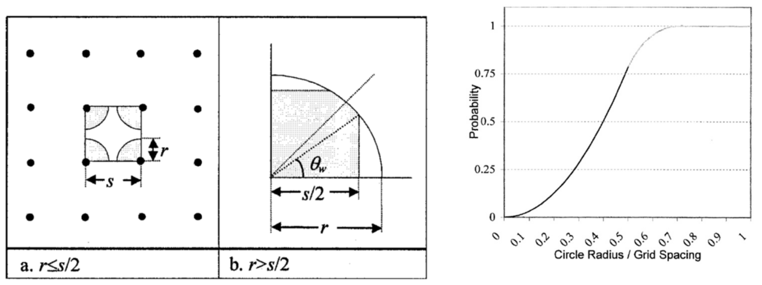
Shortridge and Goodchild [12] estimated the probability of geometric intersections between objects and tilings, particularly the probability that a circle of a given radius will intersect with gridded points. A well-known problem in rasterization is that small objects may “disappear” if no such intersect occurs. Figures from that paper (reproduced below, Figure 1) show how this probability varies with the resolution-object size ratio:

Shortridge and Goodchild [12] show that the probability of intersection follows an S curve, with an increasing slope up to about 0.5. Thereafter the curve flattens out (in a faint tone to indicate there is also overlap between the circles). The authors state that “the probability that a polygon is missed during conversion to raster is clearly a function of raster cell size and polygon shape and area”. [12]. It leaves the question of the appropriate raster representation when the circles overlap.

Visibility Analysis

Line of sight intersection occurs in a projected space with occlusion affected by view orientation and angular precision [25]; thus, it cannot be validated in the field or via test figures [26]. Angular precision matters in both raster and vector methods [27,28]. Consequently, information about uncertainty in a viewshed must be generated following Hidden Surface Removal, which is challenging for analytical purposes [26]. While typical ranges of uncertainty in viewsheds can be ascertained for a terrain model of typical topographies [29], the range of possible viewsheds is, in principle, unbounded since a minute gap in a surface can provide extensive visibility. Thus, despite improvements in speed [30], modeling uncertainty in visual analysis requires consideration of perceptual issues such as autocorrelation and scene coherence [31]. The problem is then to distinguish between Wolf’s [2] “actual” and “possible” parts. Most visual landscape classifications have modifiable partitions, but there are also higher order topologies (e.g., Euler Zones, see [31]) forming (locally) viewpoint invariant discrete partitions on the more detailed aspect graph [32], a process called graph granulation [33]. Visibility is thus one area where geographical scale effects, which are hard to statistically bound, can arise from granular effects at extremely small grain sizes.

Graph Partition and Granulation

“Any spatial partition has a corresponding dual graph” [33]. The common “dissolve” operation simplifies polygon data by combining adjacent partitions with common attributes. Implicitly the nodes of these partitions are combined into a single node in the dual graph. Subgraphs of a network partition it into a coarse-grained representation of the full graph [33]. How coarse and detailed graphs relate across scales is important for problems such as efficient route finding [34], particularly when the location of the traveler is imprecise [35].

Path Analysis

Graph granularity also affects path analysis in discreet space. For example, topology is implicit in the partial ordering of a square raster. However, Triangular Irregular Networks (TIN) usually represent topology explicitly [36], with some data structures offering more complete representations (e.g., a Quad-Edge Delaunay TIN [37]) making more directions of travel available to routing and flow algorithms. Finer orientations can be achieved by using a larger step radius [38] and multiple scales ([39]), but Goodchild [40] shows the movement is only asymptotically Euclidean with a smaller grain.

From Tilings to Lattices

Spatial overlay, intersect, visibility, flow, and network operations are all vulnerable to even minuscule uncertainties due to the binary nature of the decisions to be made at a partition. Overlay and intersect have the advantage that while errors may compound and propagate during analysis, the decision remains local to the objects concerned. In analyses such as visibility, least cost path, and flow accumulation, the error will be “transmitted” elsewhere in a manner that is hard to trace. Therefore, amplification of error by projection or accumulation is problematic, both with positional uncertainty (due to conceptual vagueness [41] or observed imprecision [42]) and topological incompleteness. For clarification, ‘uncertainty’ leaves one unsure as to degree but with some basis for estimation, whereas ‘incompleteness’ leaves one lacking knowledge.

The Region Connection Calculus (RCC) [43] is an interesting alternative model of tiling space since it both draws directly on mereology [44] and can be derived from lattice algebra [43]. Lattices are an example of partial ordering [40], which shall prove essential in Section 3. Lattices can also represent vagueness, which is “closely related to granularity” [33] since space within discrete grains at one precision may be divided by the grain at another.

2. Establishing Whether All Locations on a Map Can Be Uniquely Addressed

This brief method to answer the opening hypothesis rests on three conditions: (a) That isometric precision implies a position be defined within a radius describing a hard perimeter. (b) The shape of the function describes the probability of a unique intersection between any point and the set of available addresses. (c) What happens to that function when the resolution approaches infinity?

2.1. Unique, Spherical Address Units

By convention, precision is measured as a distance “r” in all directions, thus a circle or sphere. It is, of course, possible to map two locations closer than “r” to a precision of “r”, but doing so implies topological vagueness as it cannot be discounted that any two objects mapped as such may, in fact, be in the same place. If coordinates are considered as a three-dimensional (3D) lattice of addresses, a sphere can be defined around each point, giving a complement equivalent in radius to the measurement precision, while the lattice spacing defines coordinate resolution. Condition (a) met, the answer to the hypothesis depends on the shape of the function in (b). If it reaches one, then the hypothesis must be held as true, or it if tends asymptotically toward one, it is least arbitrarily close to being true.

The experiment in Figure 1 can now be reversed; does increasing the coordinate resolution improve the probability of locating a point on a lattice of circles asymptotically, as Shortridge and Goodchild [12] showed for locating a circle on a lattice of points? If coordinate resolution exceeds measurement precision, complements overlap so the address would be vague. If the complements “squash”, they are no longer isometric. The probability function for a unique intersection is thus limited to the bold part of the line in Figure 1, beyond this the answer depends on condition (c). As resolution tends towards infinitely high and measurement precision toward an infinitely small point, what happens to the odds that a random point will fall onto a unique address?

2.2. Kepler Conjecture

The Kepler Conjecture states that it is impossible to pack hard spheres in 3D such that the total volume enclosed by the spheres exceeds more than c74% of the total volume of their collective convex hull, more formally:

”The packing density δ (Λ) of any sphere packing Λ in R3 does not exceed π √18 ≈ 0.74048”. [45]

Hales [46] demonstrated this conjecture is probably correct. Since the conjecture and Hales’ Proof of it are confined to Euclidean space, any implications must be restricted to it. Nevertheless, within that common analytical arena, while the degree to which precision affects representational completeness may be contingent on scene coherence [29] or spatial autocorrelation [47] of the phenomena, space itself appears to not be fully addressable.

2.3. Interim Conclusions

The implication of Hales’ proof [46] is that the absolute risk of a point not finding an address is constant with resolution thus the opening hypothesis must be false. While it may be generally understood that all spatial data is only a sample, this implies something more fundamental about analytical space itself. A notion of scale-constant incompleteness would carry implications for how the relationship between Tobler’s First Law and Heterogeneity is understood, particularly for fractal phenomena [47], by placing an upper bound on the proportion of space that can be sampled independently. For a succinct overview of the relationship between ’big data’ and sphere packing see Cohn’s, Arnold Ross Lecture of 2014, (https://www.ams.org/publicoutreach/students/mathgame/cohn-slides-2014-web.pdf, accessed on 13 February 2023). Immersive, real-time applications are often close to the grain. Granularity in space-time blurs the distinction between spatial and temporal uncertainty which is generally considered to be a problem to be resolved but could prove to be the solution to this apparent paradox of a “grainy continuum”.

3. Does Time Smoothen Space?

Answering the opening hypothesis in the negative has posed an apparent paradox with theoretical and practical implications. This section will first attempt to resolve that paradox in theory and then propose a pragmatic approximation for a space-time data structure in the form of Face Centered Cubic Packing (FCCP).

3.1. Space-Time Representation

Geographical sciences have long been aware of the intimate connection between space and time [48]. Methods proposed for space-time representation include modeling spatio-temporal data as points and tracks [49], sequential stacks and semantic events [50] or as fields and surfaces, tessellated such as kinetic Voronoi diagrams [51] or discrete prisms [52] the most commonly applied of which is the space-time cube. Peuquet [53] presents a thorough theoretical overview of the issues in spatio-temporal mapping and some early modeling approaches, which remains remarkably current. Ohori et al. [54] provide a more recent review of spatio-temporal models in GIS. They identify several additional approaches to those mentioned (composite methods, object-oriented models, and some conceptual and semantic models) but conclude that most consider time to be a distinct dimension onto which snapshots or events are to be mapped. These approaches to modeling space-time are perhaps better described as 3D + 1 since the time dimension is not topologically integrated (at least not in four dimensions, prisms have been implemented with time as the third dimension either as part of the object or by extrusion). Ohori et al. [54] present a 4D model of space-time prisms based on topological vector objects, arguing that “true” 4D requires time to be topologically integrated with space. Prior work that does this includes the 4D partitioning approach of Erwig and Schneider [55] and the fuzzy space-time coordinates of Brimicombe [56]. More recently, Nesani Samany et al. proposed the Fuzzy Spatio-Temporal Prism [57]. All these methods start from a “monist” [58] assumption of an extant space over which partitioning events unfold. There is also a long-standing approach whereby space-time is “constructed” from discrete elements, beginning well before the famous discussions of Newton, Leibnitz, and Clarke on the relationship between space, time, and continuity. This approach will be taken below, but what properties need to be considered? As the aim is only a consideration of space-time as an information formalism, not its physical existence [59], it seems reasonable to focus on the peculiar properties of time identified by Peuquet [53] as of relevance to GIS:

• Time is directional (the arrow of time);
• Chaotic behavior may amplify small uncertainties through time;
• Relative space and time are subjective, and neither exists independently;
• Both space and time are generally conceived as continuous, yet for purposes of objective measurement, they are conventionally broken into discrete units;
• Temporal data is often incomplete. Science has traditionally viewed incompleteness as something to be overcome rather than to be openly acknowledged or willingly incorporated into models as a basic characteristic.

(Summarized by Peuquet [53]).

Property (d) expresses the “grainy-continuum” paradox. The next section sets out a method (logical argument) for how discrete elements may generate a continuous space in which the other properties are innate.

3.2. Time as Relative Dimension in Space

3.2.1. Premises

The work of mathematician Roger Penrose introduces a number of important concepts and principles which are central to the later arguments pursued here:

A necessary constraint is ”to get rid of the continuum and build up physical [… read spatial…] theory from discreteness”. [60]

One should “concentrate only on things which, in fact, are discrete in existing theory and try and use them as primary concepts—then to build up other things using these discrete primary concepts as the basic building blocks. Continuous concepts could emerge in a limit, when we take more and more complicated systems”. [61]

”The most obvious physical concept that one has to start with…and which is connected with the structure of space-time in a very intimate way, is in angular momentum”. [60]

However, despite the importance of Penrose’s thinking to this work and some apparent parallels with problems in physics, like Penrose: “the picture I want to give here is just a model… I certainly don’t want to suggest that the universe ‘is’ this picture or anything like that”. [60].

3.2.2. Building Dimensions

Consider two or more observations that are measurably distinct, i.e., a “natural” topology of real numbers [62]. To establish an order of change a third is needed, a triad [63] (not to be confused with Peuquet’s triad of locations, times, and objects [48]), which may connect as a graph [64]. A random graph [65] un-directed and without pre-assigned global characteristics (such as dimensions or convexity) ensures no implicit background.

3.2.3. Building a Probabilistically Continuous Dimension from a Graph

The “threshold of connectivity” of a random graph is the number of edges needed for there to be a strong probability all nodes in the graph are connected [65], e.g., for a binomial random graph “G(n,p) at p(n) = log n/n” [66]. The number of spanning trees of a connected graph is an invariant Nⁿ⁻² as given by Cayley’s formula [67], but every connected graph contains at least one spanning tree [68], (theorem 4.12). It is thus always possible for such a connected graph to randomly form an ordered set [66] (e.g., a tuple, line, or tree, etc.) where every node has a unique matrix of graph distance to all other nodes. If such a graph describes the diffusion of information throughout a network, then the maximum “time” (in a number of moves) it could take for information to diffuse throughout the network is when the spanning tree is an Euler path. Simple paths between other nodes will therefore require some fraction of this maximum. The probability of a topological chain (a tuple) of length no greater than i to form a path between any two particular nodes is given by Equation (1):

$$P_i=\frac{2}{n}+{\displaystyle \sum }_{v=2}^i \frac{1}{n_v}$$

(1)

P = probability of a path between two points being achieved in i random steps where v = v^th node added to the path; n = total nodes. i.e., the initial chance of a direct connection (P = 2/n) plus the sequential sum of the chances that each further node added (v) to the chain will be the destination, each such chance being 1/n.

In Equation (1), each ith additional node on the path increases the chance of a complete path by 1/n since nodes already in the path are still available. In this way, information moves over/through the graph by a node randomly swapping its position in the graph to create the path.

3.2.4. Topological Rotation

Consider a simple graph where one node connects all the others directly. Thus, others have a graph distance from each other of two. Given a constant metric per edge, these points can describe a circular arc in two dimensions (2D), while one point sits at the center, i.e., a wheel graph [69]. Abstracting this further (a circulant [24]), the concept of rotation in a topological sense is known as an “orbit” of the node under “group action”, a subset of which “fix” the node by returning the system to its original state [70]. So even without literal “spinning”, the concept of total angular momentum is relevant, and the term will be used for convenience to denote the ability of a node to swap position. The total momentum M is thus the set of all possible orbits (hereafter, one “revolution” of the system). The maximum relative “speed” information may attain over such a graph is the shortest path forming an arc of an orbit. How “fast” that arc might be transited, relative to some external clock, is irrelevant but cannot be infinitely fast since if the start is returned to instantly, no change can be observed (contradicting the natural topology premise [62]). With the property of angular momentum paths may not be equally likely:

$$P_{ij}=\frac{2m_i{m}_j}{M}+{\displaystyle \sum }_{v=2}^a \frac{m_v{m}_a}{M}$$

(2)

P = probability of a path; i = start node; j = end node; v = next node added; a = the node completing the path to the destination; m = a node with momentum; M = total angular momentum of the system.

In Equation (2), the probability of a direct path (P) forming is for two nodes i and j connecting directly, given their fraction of the total momentum of the system M. For a path of three or more nodes, one must then add the sequential sum of the probability (in proportion to M) that each subsequent node added to the tuple will complete the path directly to m_j.

3.2.5. Conservation of Momentum

The analogy may be extended to the conservation of angular momentum by instead considering m as the amount of information flowing through nodes to evenly distribute M, forming a signal across the graph [24]. A higher net momentum between nodes means more frequent (“briefer”) interactions but also a higher probability of new connections, thus a locally faster transmission rate (i.e., clustering [71]). The relationship between each cluster and the full set is given by Equation (3):

$$\exists \mathcal{M} m_i^j\sim d\in P,M\sim D,n\subseteq N \forall i,j\in n\in \mathcal{M}$$

(3)

i.e., there exists a set of points M, such that for any subgraph n and any points i, j on n, the angular momentum m_ij follows distribution d defined by probabilities P (from Equation (2)), and total angular momentum M follows distribution D, and each subgraph n belongs to a set of points N.

The probability of distribution $m_j^i ~d$ (hereafter f) existing on D will then be the Cauchy product (or the discrete convolution) of f and M~D (the probability distribution of M here after g) in Equation (4):

$$\left(f\ast g\right)\left[n_m\left]={\displaystyle \sum }_{m=0}^M f\left[m\right]g\right[n_m-m\right]$$

(4)

i.e., the probability of a distribution of momentum within subgraph f being formed across the parent set g on n discrete elements in common of momentum m respectively is the discrete convolution f ∗ g.

In the simplest case, f is just an Euler path over g formed at random as per Equation (2). As m accumulates into f, so too does the probability of a path existing between i and j. Implicit here is that membership of a subgraph is defined by connection, i.e., f is a consistently connected graph while g may not be. The more the momentum concentrates into some subgraphs over others, the more the overall graph becomes structured, and the passage of information over the N subgraphs takes on a structured number of steps, i.e., some branches become probabilistically more distant relative to others.

3.2.6. A Lattice of Communication

The individual nodes in the graph have no spatial relationship (they are not embedded in space at all), but they constitute a network over which information travels in discrete steps. However, in principle, the relative communication time between one node and all others is continuous. Any number of nodes may be transited en route, and these may have any relative angular momentum, so any fraction in communication time is possible. The distribution of momentum values possible is discrete (being divided over nodes in the graph). However, the metric of communication time, being based on arbitrary ratios of frequencies, may include complex and irrational numbers ([72] p.14) so the emergent dimension of “Lattice Communication Time” (LCT) is genuinely continuous. Each path between two nodes on the graph can thus be mapped as a vector between points in this continuous, latent hyperspace.

The spatial representation of diffusion of signals on a graph, which partitions it into regions, is known as Graph Spectral Decomposition, in which “the Laplacian encodes a notion of smoothness on a graph” [24] (for a good introduction, see, Knyanzev, B, Spectral Graph Convolution Explained and Implemented Step By Step. https://towardsdatascience.com/spectral-graph-convolution-explained-and-implemented-step-by-step-2e495b57f801 accessed on 4 June 2021).

It is clear from Equation (2) that time t for path ij is a probabilistic fraction of M (the LCT domain). Similarly, the relative “volume” of f to g is bounded by the proportion of M in f if both are connected. But g is not necessarily a connected graph. Consider a case where every node in g has equal momentum and connects to another node, or not, at random. Over enough iterations, the mean graph distance between all nodes would be equal. The only geometric projection for this is if all nodes are at the same (fuzzy) point. Branching into connected subgraphs represents a divergence from such a low-order state, e.g., a branch may be a path to a leaf node which, though multi-step, is still more probable than the leaf node connecting directly to any other node in G (Equation (5)):

$$P_{ij}>P_{iv} \forall t_{ij}=\frac{m_{ij}}{M}\in {\mathcal{F}}_{ij}\in \mathbb{G} \forall v\in \mathbb{G}:v\notin {\mathcal{F}}_{ij}$$

(5)

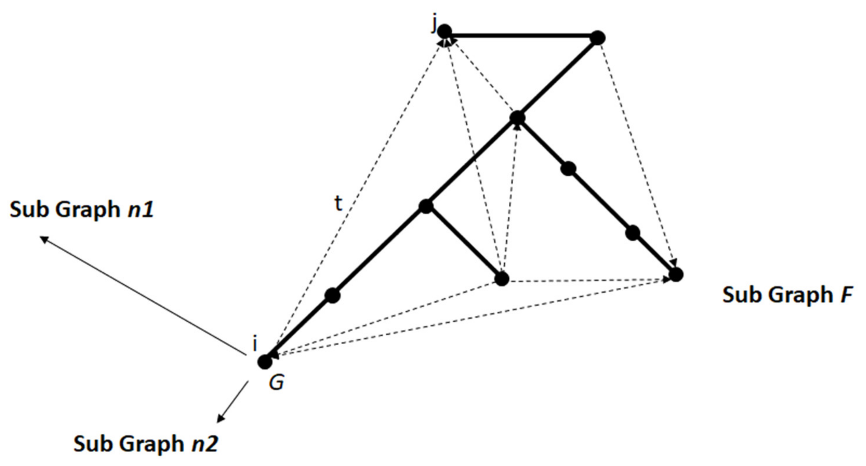
$\mathcal{F}$is a vector space of the LCT of a subgraph on $\mathbb{G}$ containing a path between nodes ij with momentum m. v is any node in $\mathbb{G}$, not in $\mathcal{F}$. $t_{ij}$ is the LCT vector for path ij of length equal to the proportion of the domain M constituted by m_ij. For all cases where this is so, the probability P of the path ij is such that ij has a greater probability than iv.

Equation (5) defines the condition at which a path P_ij becomes more probable than alternative paths from i to v. Figure 2 illustrates this, but by taking a node i, which projects to the same point in LCT space as the rest of G and a path from this node to j, which is reached via some structured route therefrom. This divergence “stretches” G from its projected point-like form into a vector. Other branches are added to illustrate that if structured paths exist from j to other points, these could also project to vectors which, in this simple case, are resolvable in 2D (Figure 2).

Although relative speed is analogous to distance, $G$ is a hyper-space with complex topology and relative positions, not a spatial volume such as ${ℝ}^{\mathrm{n}}$ with absolute locations; but it has the potential to be similar. Consider the outcome that a single packet of information happens to take a route from one node in the graph to every other node through a single chain with no loops. $G$ would be a 1D ordinal series of nodes with equal LCT time difference, i.e., a scalar vector. If each node has differing angular momentum, then sections of this vector would take different lengths of “time” to cross (per Equation (2)). Either way a continuous spatial dimension can emerge, in the latent space [71], on a random graph. The LCT field is scalar, but an emergent space with independent dimensions is more particular.

3.2.7. Building a Probabilistically Continuous Volume

Additional dimensions result from the graph entering a state, requiring a new Linearly Independent Vector through the LCT. Carrell [73] defines a LIV thus:

“a set of vectors is linearly independent if no one of them can be expressed as a linear combination of the others” [73], p. 116.

If a cycle exists with three or more nodes, then each direction of rotation over that cycle represents different orderings of linear combinations of two independent vectors in any LCT metric space such that the sums are the same, i.e., it needs two dimensions to represent it geometrically. Carrell (ibid) further states that:

“F_n can’t contain more than n independent vectors. Our definition of dimension will in fact amount to saying that the dimension of an F-vector space V is the maximal number of independent vectors. This definition gives the right answer for the dimension of a line (one), a plane (two) and more generally F_n (n)”. [73], p. 121.

To resolve the LCT into projected space, a new dimension must be added whenever some combination of the existing independent vectors cannot complete a path. There remains the question of the precision of that space in all dependent vectors through it (Equation (6)):

$$\mathbb{P}\equiv {\displaystyle \sum }_{V\in {\mathsf{T}}_{pn}\in \mathcal{F}}\left(V\oplus V\right)$$

(6)

i.e., A manifold ${\mathbb{P}}^{ }$ is the direct sum of V independent vectors (each comprising a tuple ${\rm T}$ of n nodes with a probability p of existing (given by Equation (2)) over a discrete scalar field ${\mathcal{F}}^{ }$.

3.2.8. Precision in Projected Space

Although discrete elements of each dimension are composed only of topological elements with non-oriented angular momentum, they now also have a probabilistic ordering in LCT and so must occupy a discrete position in the LCT to some rational interval. If achieving this requires the LCT to be resolved into more than one dimension, then so too must that interval. Thus, the problem is not simply one of ordering nodes in one dimension but of packing them in two or more dimensions and thus also packing their circular, spherical, or hyper-spherical error margin.

Let ${\mathbb{P}}^{ }$ from Equation (6) be one instantiation of the metric space of the LCT and ${{\rm T}}_{pn}$a tuple on that space. Each element e of that tuple ${{\rm T}}_{pn}$ has a spherical margin of error of radius r around it (Equation (7)):

$$e=B\equiv \left\{x,y\in \mathbb{P}|d\left(x,y\right)\le r\right\} \forall e\in \mathbb{P}$$

(7)

Each element e of the metric space ${\mathbb{P}}^{ }$ is B, which has the dimensions dx, dy (being less than or equal to radius r).

As per Kepler’s conjecture, no packing of B can fill space, but this can be resolved by recognizing that there is indeed the possibility for every relative position in LCT, but not every vector can be embedded to a common absolute precision in ${ℝ}^{\mathrm{n}}$ simultaneously. Thus, if the graph topology to resolve the LCT requires ${ℝ}^{\mathrm{n}}$ for a continuous space, realizing this requires at least ${ℝ}^{\mathrm{n}+1}$. Another way of viewing this conclusion is to say that the lattice in ${ℝ}^{\mathrm{n}}$ represents the most complete (probable) mapping between LCT and ${ℝ}^{\mathrm{n}}$ achievable.

The most efficient 3D packing structure is hexagonal [74], such that each higher dimension places nodes at the center of the dual for the mesh in the dimension below it, which is also the center for the interstitial space. Expressed formally (Equation (8)):

$$\left(B_1^n\cap B_2^n\ne \varnothing \right)\to B_2=V\equiv B_1^{\star }\in {\mathbb{P}}^{n+1}$$

(8)

If the finite complement B of two elements intersects in n-dimensional space, then B₂ must be an element of the B_1,2 vector dual V in the next dimension in ${\mathbb{P}}^{ }$.

Some of the points in the projected map may have vague topology in 3D space alone, but it is explicitly recognized that only one of the possible nearest conditions to this may be defined at any one time. Any subset of the higher dimensional LCT may be “foregrounded” [75] in the projected partition, so no vector is ever impossible, but others must be “traced over” [75].

3.3. Stability of the LCT

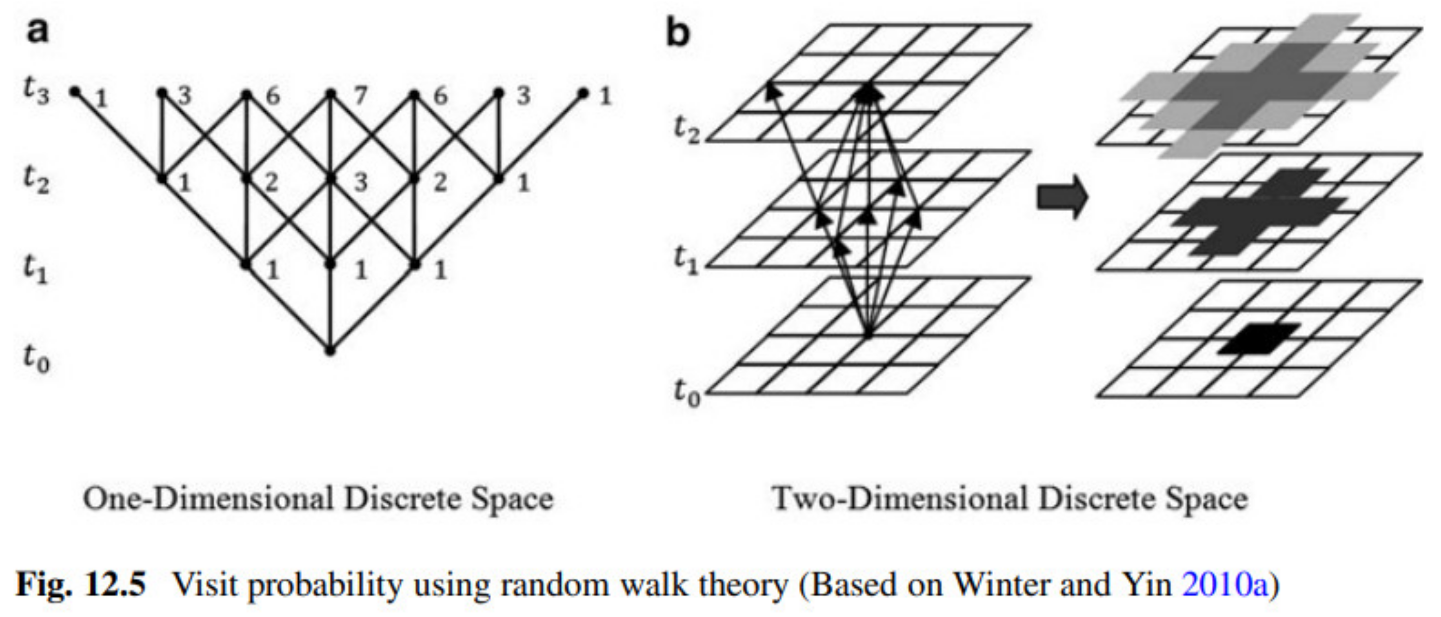
Vectors in LCT are not created by the passing of a packet of momentum between two nodes but by the ordered passing of that packet across many nodes. Relative LCT distance and position are the results of net relative connection speed across all nodes in the graph. Most probable is thus mapped as most direct, as per random walk theory [76] (Figure 3):

Straight vectors in LCT represent the most probable path given the angular momentum distribution, so following the principle of least action [77], Feyman’s [78] path integral formula can be applied. Let T be a tuple with a Gaussian probability of describing the shortest path over the field $\mathcal{F}$ (from Equation (6)). Let V be a linear vector in $\mathcal{F}$ having the same start x_a and endpoint x_b as T (Equation (9)):

$$P_t(C(V_x\cap T_x)\ne \varnothing )=P((({{\displaystyle \int }}_{\mathrm{x}\left(0\right)=\mathrm{x}}^{\mathrm{x}\left(\mathrm{\tau }\right)=y} \mathcal{D}xexp(-{{\displaystyle \int }}_0^t \frac{x^2}{2}dt)-V)\ne 0)\le \left(1/2\right)$$

(9)

i.e., the probability $P$ at an instance t that the Complement $\complement$to the intersection between the elements of the straight line V and the elements of the Tuple T is not empty (and thus the path taken was not linear) is equal to the probability that the integral path dt of the vector of a free particle moving from x_a to x_b over $\mathrm{\tau }$ convolutions, minus the straight-line vector V = [x_a x_b] does not equal zero given a potential set of paths $\mathcal{D}\mathrm{xy}$. $P$ must have a value equal to or less than 0.5 since, for a Gaussian distribution, a linear route is more probable than an indirect route.

The implication of Equation (9) is that a straight line is the most probable path over the LCT. A node is only likely to resolve into ${ℝ}^3$ when it provides an important link between many points in the LCT rather than a “tunnel” between just two points. If only considering an instant, the projected LCT is timeless and granular. Smoothness results from iterations reordering the packing topology. So to be strictly accurate, it is “iteration” rather than time that smooths space. Thus, “over time” discrete space (d) becomes smoother (i.e., 3d^t ≃ 4D). This “topological time” is conjugate with the three spatial dimensions; it is not an independent “arrow” of time but Rovelli [79] shows the traditional sense of time as an independent dimension directing “progression” could be emergent from partial ordering effects at each spatial scale.

3.4. Summary

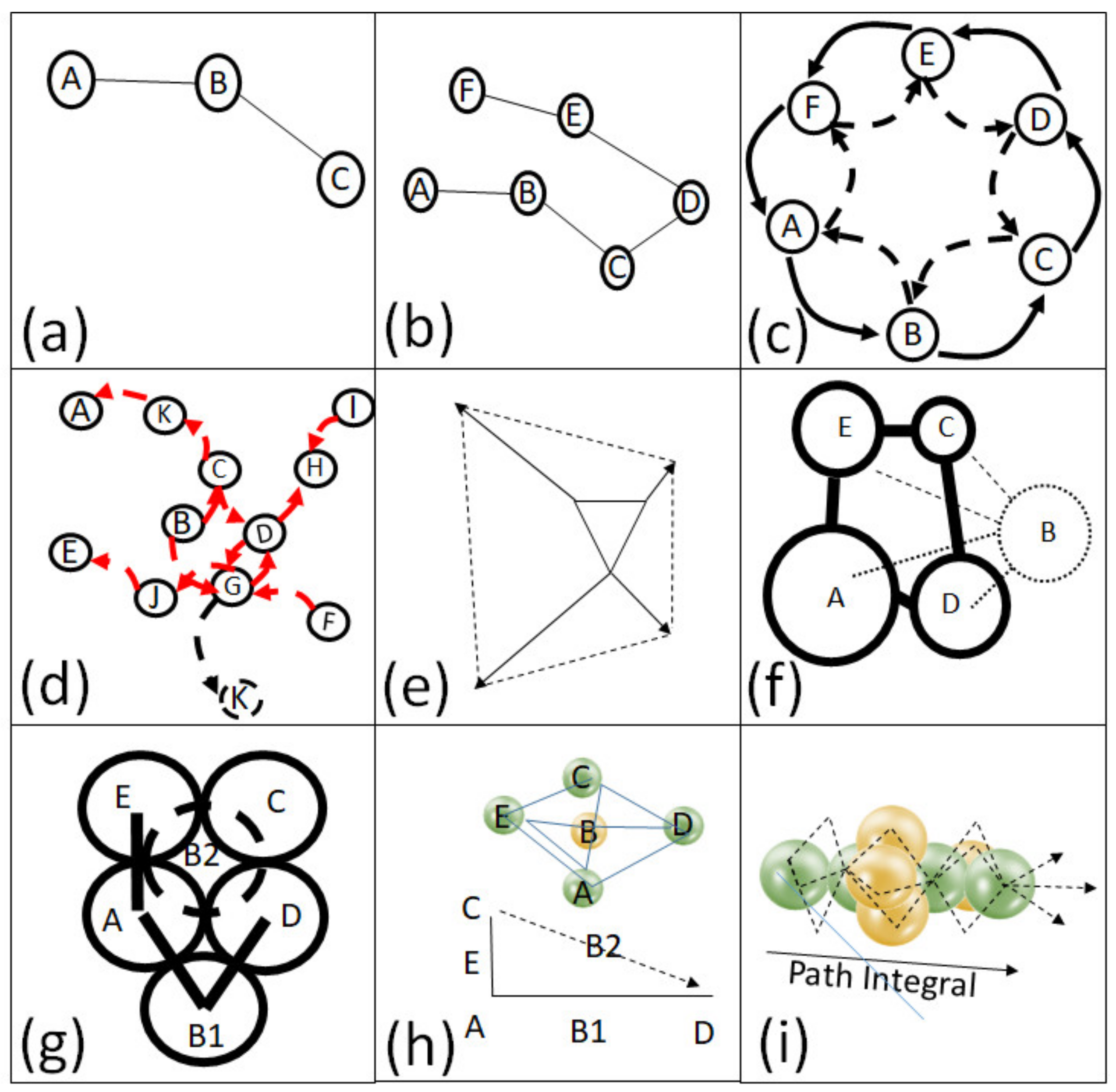
The core proposition of this section is that from a random graph, a latent field may emerge, which is a spatial continuum in the sense of addressing any set of relative spatial relations to isometric precision but sphere packing imposes a grain when projected into absolute Euclidean location. This grain may be “smoothened” by iteration, resulting in the emergence of a fuzzy space-time continuum. Figure 4 summarizes these steps:

Section 3.2 and Section 4.2 are explained in detail in Supplementary Materials.

4. Discussion: From a Dynamic LCT to a Computable Lattice

4.1. Implications for Space-Time Representation

The process of attempting to build, rather than define, a continuous space from discrete elements reveals, mechanistically, implications of the points (a,e) by Peuquet [53] in Section 1, on which basis several ideals for space-time representation may be noted:

• Ideally, use discrete units which can be “smoothly” space-filling. (d,e);
• Ideally, represent incompleteness and non-commutativity. (a,c,e);
• Ideally, use isometric grains. (b);
• Ideally, represent granular space-time conjugation explicitly. (c);
• Ideally, represent local uncertainty in causality while respecting causality globally. (a) (Galton et al. [80] observe that “granularity effects may often confound an attempt to derive strict causation”).

A graph with emergent LCT appears to overcome some of the apparent contradictions in these ideals. The LCT is fundamentally smooth but discreetly addressed by the graph. Incompleteness is inherent in that only spatial relations within the graph are defined (there is no question to be asked as to the location of “empty space”). Uncertainty is isometric along the edges of the graph, and space-time is locally conjugate, but global causality emerges. However, a fuzzily-emergent space has obvious flaws as a spatial data structure. Even were it feasible to compute an emergent LCT, it is dynamic and a projection in ${ℝ}^{\mathrm{n}}$ only remains smooth so long as it contains little data. There is no escaping entirely Kepler’s conjecture on sphere packing. So what is the best approximation in a simple, static lattice?

4.2. FCCP for Space-Time Representation

The central issues are how to best minimize anisometric uncertainty and normalize it between space and time, how to represent spatio-temporal conjugation, and what to do with the incomplete part.

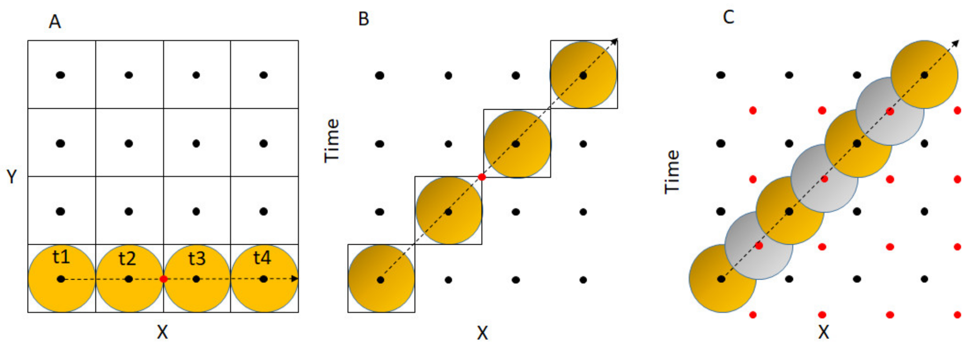
If time is simply recorded as a non-geometric time stamp, then uncertainty in the time at which the trajectory crosses from one unit of space to the next is not represented (red point in Figure 5A). In a space-time prism (Figure 5B), rational units are maintained for change in space or time but not both. Geometrically this is no different from 2D raster tiling being non-isomorphic. However, this is arguably more fundamental in space-time because movement can only happen simultaneously in both spatial and temporal dimensions i.e., it will always be over non-axial vectors in space-time (it is not diagonalizable).

Hexagonal data structures [81] are more information-dense than Cartesian coordinates but also less convenient to represent in a computer. Voronoi-Delaunay triangulation could also represent a hexagonal data structure [82] but computation for 4D would be hard [54]. A simpler option, easily applied to fields, is to use a Cartesian array but offset the origin for alternate layers (a Face Centered Cubic Packing, FCCP) and define the offset layers as representing spatio-temporal uncertainty between the non-offset layers and vice versa (Figure 5C). In effect, this interweaves two offset space-time cubes, each of which provides topology for observations that are uncertain on the grain of the other. Conceptually challenging but computationally trivial.

Peuquet suggests (in 2001, but the point remains valid) that the slow progress in addressing temporal aspects of GIS is partly because “historically there has been a general emphasis on the short-term and implementation-oriented solution” [53]. FCCP is suggested here simply to encourage discussion, not asserted as the solution, and whether a simple array or a 4D mesh would be an appropriate implementation depends on the application. However, a general test of the principle would be what proportion of spatio-temporal data points (and any imputed midway points) can be unambiguously addressed to a constant accuracy in FCCP compared to other data structures.

5. Conclusions

5.1. On the Representation of Time

Langran suggests that all maps have a temporal reference, even if only an implicit ‘now’ [83]. The increasingly real-time nature of data sources highlights that maps usually cover a period of collection, which has traditionally been allocated a publication date. Generalizing a period to a single timestamp is equivalent to an orthographic projection because all points in time project to the same plane, rather as height on a 2D map. The scale ratio between spatial and temporal dimensions is, effectively, a foreshortening effect, so determining square units is important. Considering analyses such as spatio-temporal clustering, is 2m 2s away closer than 1m 3s? How equivalent are uncertainties in space and time for point-in-prism analyses [52] or object-based view-shed analyses [25] where inter-visibility is dependent on temporal factors? If detecting motion in discrete space [84], should one assume a linear, constant motion within each grain or consider a straight line to be the lower bound [85] on a probability function in position [75]? All are examples where the spatial-to-temporal scale relationship might amplify uncertainty. In calling for greater attention to the development of a theory of space-time representation, Peuquet highlights the relation between continuous and discrete space, in particular when handling inexactness, interpolation for incompleteness, and multiple histories [53], all of which have been encountered here:

Computable representation of space-time: How does the selection of an optimal grain size reflect the fact that there may be a non-linear uncertainty between a measurement made too early or too late, e.g., as to the position of a shadow at noon, which itself varies over seasons, scales and locations? Consider also how spatio-temporal conjugation affects the examples from Section 1. Intersect becomes intercept, at the grain precision in measuring speed must offset precision in estimating location. Visibility Analysis becomes not just a matter of where there is a line of sight but when and for how long. Graph granulation is commonly applied to space-time applications, but doing so with vague location [35] means spatial and temporal uncertainty are not independent. Goodchild’s [40] early work on path analysis must surely come into play, but whether 4D lattice paths tend to the Euclidean length in the same asymptotical manner is an open question;

Incompleteness: Hales’ proof [46] undermines the principle that absolute vs. discrete space is a matter of differentiation alone; precision-independent incompleteness needs further exploration;

Spatio-Temporal Scale(s): Although Peuquet agrees, “it usually does not make sense to measure time in meters or feet”, [53] the point has been moot since 1960 when the meter was defined in wavelengths of light. Perhaps the distinction between meters and the time by which they are measured over-complicates space-time for 4D models? One would not, after all, model a terrain’s height on a different mathematical base to its horizontal distance. On the other hand, seconds are not fundamental scientific units either, one might ask “seconds per what?” (Smart, see Harrison [59]).

The term “related” in Tobler’s First Law implies some common point of causation or interaction, an interpretation supported by t Tobler “invoking” his first Law in the context of prediction from trend. [86]. But Galton points out that “At geographical scales… change is mostly much slower than at the scale of individual humans” [4]. Could this suggest a more general, unified interpretation of Tobler’s First Law; near things are more contemporaneously related than distant things? For example, the erosion of sand on a beach by a single rainstorm and the formation of a river delta by millennia of rainstorms shows how time scale becomes spatially embedded across spatial scales within a reference frame as to the speed of the phenomenon i.e., time operates locally to the phenomena.

The concept of a “time cone” or “light cone” is well known from physics [79]. One might then term this consequent spatial pattern a “time shadow” from layers of past moments projecting onto our present (credit: Robert Mann for the term). In this view, probabilistic, spatio-temporal change could be modeled as “time-sheds” via multiple views linked by the “shadows” cast from different viewpoints [25] with time as the “z” axis of perspective projection.

Identifying the correct reference frame [20] could be key to finding a ratio by which to normalize spatial and temporal scales. For fractal phenomena, the fractal dimension seems like an obvious candidate for investigation. Spatial scientists have the advantage of not needing to determine “plank units” which function for all cases. However, a sound theoretical basis for determining square spatio-temporal units suitable to a given dataset or phenomenon would be useful, as would theory for how within these grains space and time become probabilistically conjugate.

5.2. On Granularity and the Emergence of Spatial Smoothness

The paradox of a continuous volume, defined by relative position yet which cannot be filled by discrete positions, may have a partial solution as presented here, but this paper can only hope to add a little further weight of logical argument to the idea’s long history. Mathematical proof, if indeed possible, is of huge complexity, as would be any implementation. Nonetheless, it serves to clarify why a continuous space must be the product of a process and not a static condition. Progression through time happens in our minds when we observe [79]. Information space-time is not absolute but an analytical product.

This shift in perspective is also valuable if it encourages thinking beyond the Cartesian array to the idea of coordinates as data structures that crystallize an information space. Interestingly, this need not lead to the abandonment of simple data structures such as arrays, but there seems to be much to explore. Perhaps a-periodic tiling and quasi-crystals present options for avoiding periodic sample bias or better approximating Euclidean paths?

The most intriguing idea arising from this work is that time may act as a “smoothing” function on discrete space. Discussion within GIS on discreteness versus continuity generally rests epistemologically on Euclidean geometry and set theory. Yet, to draw the thread from Wolf’s “possible parts” [2,3], Bittner and Smith [75] observe that set theory creates object discontinuity under membership change, and we move from MAUP to a Modifiable Temporal Unit Problem [5]. FCCP offers a simple update to the space-time cube that “sutures together” time slices via interstitial topology, reducing object discontinuity.

As one anonymous reviewer pointed out, “it is often claimed that space and time cannot be separated in the context of geographical information… but a proof is lacking”. This paper provides a step toward that proof, but there is work to be done. If “the relationship between the discrete space of computation and idealized continuous space is… important for GIS” [44], perhaps the arrival in mainstream usage of real-time, immersive, spatio-temporal mapping is an opportune moment to reexamine some key tenets as to their suitability for space-time representation?

References

- Duckham, M.; Mason, K.; Stell, J.; Worboys, M. A formal approach to imperfection in geographic information. Comput. Environ. Urban Syst. 2001, 25, 89–103. [Google Scholar] [CrossRef]
- Wolff, C. Philosophia Prima, Sive Ontologia, Methodo Scientifica Pertractata; Renger: Frankfurt, Germany, 1730. [Google Scholar]
- Camposampiero, M.F. Mereology and mathematics: Christian Wolff’s foundational programme. Br. J. Hist. Philos. 2019, 27, 1151–1172. [Google Scholar] [CrossRef]
- Galton, A. Space, Time and the Representation of Geographical Reality. In The Philosophy of GIS. Springer Geography; Tambassi, T., Ed.; Springer: Cham, Switzerland, 2019. [Google Scholar] [CrossRef]
- Cheng, T.; Adepeju, M. Modifiable Temporal Unit Problem (MTUP) and Its Effect on Space-Time Cluster Detection. PLoS ONE 2014, 9, e100465. [Google Scholar] [CrossRef] [PubMed]
- Clementini, E.; Di Felice, P. A comparison of methods for representing topological relationships. In Information Sciences—Applications; Elsevier: Amsterdam, The Netherlands, 1995; Volume 3, pp. 149–178. ISSN 1069-0115. [Google Scholar] [CrossRef]
- Egenhofer, M.J.; Franoza, R.D. Point Set Topological Spatial Relations. Int. J. Geogr. Inf. Syst. 1990, 5, 161–174. [Google Scholar] [CrossRef]
- Herring, J.R. The Mathematical Modeling of Spatial and Non-Spatial Information in Geographic Information Systems. In Cognitive and Linguistic Aspects of Geographic Space; Mark, D.M., Frank, A.U., Eds.; NATO ASI Series (Series D: Behavioural and Social Sciences); Springer: Dordrecht, Netherlands, 1991; Volume 63. [Google Scholar] [CrossRef]
- Arhangel’skii, A.; Dranishnikov, A.P. S Alexandroff and Topology: An introductory note. Topol. Its Appl. 1997, 80, 1–6. Available online: https://core.ac.uk/download/pdf/82183281.pdf (accessed on 28 February 2023). [CrossRef]
- Klain, D.; Rota, G. Introduction to Geometric Probability; Cambridge University Press: Cambridge, UK, 1997. [Google Scholar]
- Solomon, H. Geometric Probability. In CBMS-NSF Regional Conference Series in Applied Mathematics, 28 (Philadelphia: Society for Industrial and Applied Mathematics); Stanford University: Stanford, CA, USA, 1978. [Google Scholar]
- Shortridge, A.; Goodchild, M. Geometric probability and GIS: Some applications for the statistics of intersections. Int. J. Geogr. Inf. Sci. 2002, 16, 227–243. [Google Scholar] [CrossRef]
- Egenhofer, M.; Clementini, E.; di Felice, P. Topological relations between regions with holes. Int. J. Geogr. Inf. Syst. 1994, 8, 129–142. [Google Scholar] [CrossRef]
- Winter, S.; Frank, A. Topology in Raster and Vector Representation. GeoInformatica 2000, 4, 35–65. [Google Scholar] [CrossRef]
- Watson, S. The number of complements in the lattice of topologies on a fixed set. Topol. Its Appl. 1994, 55, 101–125. [Google Scholar] [CrossRef]
- Lindsay, J.B. The practice of DEM stream burning revisited. Earth Surf. Process. Landforms 2016, 41, 658–668. [Google Scholar] [CrossRef]
- Worboys, M.; Duckham, M. GIS: A Computing Perspective, 2nd ed.; CRC press: Routledge, UK, 2004; ISBN 9780415283755. [Google Scholar]
- Goodchild, M. Measurement-based GIS. In Spatial Data Quality; Shi, W., Fisher, P.F., Goodchild, M.F., Eds.; CRC Press: Boca Raton, FL, USA, 2002; ISBN 9780429219610. [Google Scholar]
- Monmonier, M. Geocoding, in The History of Cartography, Volume 6 Cartography in the Twentieth Century, Edited by Mark Monmonier. 2015. Available online: https://press.uchicago.edu/books/hoc/hoc_v6/hoc_volume6_g.pdf (accessed on 8 June 2021).
- Tobler, W. Frame independent spatial analysis. In The Accuracy of Spatial Databases; Michael, F., Goodchild, S.G., Eds.; Imprint CRC Press: Boca Raton, FL, USA, 1989; Available online: https://www.taylorfrancis.com/chapters/edit/10.1201/b12612-22/frame-independent-spatial-analysis-waldo-tobler (accessed on 28 February 2023)ISBN 9780429208317.
- Siddharthan, R. The Uncertainty Principle for Dummies. 1998. Available online: https://www.imsc.res.in/~rsidd/papers/uncert.pdf (accessed on 6 March 2023).
- Goodchild, M.; Mark, D. The invertibility of distance matrices. In Geographical Systems and Systems of Geography: Essays in Honour of William Warntz; Coffey, W., Ed.; Department of Geography, University of Western Ontario: London, ON, Canada, 1988; pp. 141–151. [Google Scholar]
- Stage, A.; Salas, C. Interactions of Elevation, Aspect, and Slope in Models of Forest Species Composition and Productivity. In For. Sci.; 2007; 53, p. 4. Available online: https://www.fs.usda.gov/rm/pubs_other/rmrs_2007_stage_a002.pdf (accessed on 28 February 2023).
- Agaskar, A.; Lu, Y. A Spectral Graph Uncertainty Principle. IEEE Trans. Inf. Theory 2013, 59, 4338–4356. [Google Scholar] [CrossRef]
- Sang, N.; Gold, C.; Miller, D. The topological viewshed: Embedding topological pointers into digital terrain models to improve GIS capability for visual landscape analysis. Int. J. Digit. Earth 2016, 9, 1185–1205. [Google Scholar] [CrossRef]
- Fisher, P. Algorithm and implementation uncertainty in viewshed analysis. Int. J. Geogr. Inf. Syst. 1993, 7, 331–347. [Google Scholar] [CrossRef]
- Coll, N.; Fort, M.; Madern, N.; Sellarès, J. Multi-visibility maps of triangulated terrains. Int. J. Geogr. Inf. Sci. 2007, 21, 1115–1134. [Google Scholar] [CrossRef]
- Watt, A. 3D Computer Graphics; Addison-Wesley: Boston, MA, USA, 2000; Volume 570, pp. 1–13. [Google Scholar]
- Nackaerts, K.; Govers, G.; van Orshoven, J. Accuracy assessment of probabilistic visibilities. Int. J. Geogr. Inf. Sci. 1999, 13, 709–721. [Google Scholar] [CrossRef]
- Carver, S.; Washtell, J. Real-time visibility analysis and rapid viewshed calculation using a voxel-based modelling approach. In Proceedings of the Twentieth Annual GIS Research UK Conference, Lancaster, UK, 11–13 April 2012. [Google Scholar]
- Sang, N.; Hägerhäll, C.; Ode, Å. The Euler character: A new type of visual landscape metric? Environ. Plan. B: Plan. Des. 2015, 42, 110–132. [Google Scholar] [CrossRef]
- Plantinga, H.; Dyer, C.R. Visibility, occlusion, and the aspect graph. Int. J. Comput. Vision 1990, 5, 137–160. [Google Scholar] [CrossRef]
- Stell, J. Granulation for Graphs, Spatial Information Theory. In Cognitive and Computational Foundations of Geographic Information Science. International Conference COSIT’99 of Lecture Notes in Computer Science; Freska, C., Mark, D., Eds.; Springer: London, UK, 1999; Volume 1661. [Google Scholar]
- Timpf, S.; Kuhn, W. Granularity Transformations in Wayfinding. In Spatial Cognition III, Lecture Notes in Computer Science (Lecture Notes in Artificial Intelligence); Freksa, C., Brauer, W., Habel, C., Wender, K.F., Eds.; Springer: Berlin/Heidelberg, Germany, 2003; Volume 2685. [Google Scholar] [CrossRef]
- Duckham, M.; Kulik, L.; Worboys, M. Imprecise Navigation. Geoinformatica 2003, 7, 79–94. Available online: http://duckham.org/matt/wp-content/uploads/2020/11/Imprecise-navigation.pdf (accessed on 6 March 2023). [CrossRef]
- Gold, C. Tessellations in GIS: Part I—Putting it all together. Geo-Spat. Inf. Sci. 2016, 19, 9–25. [Google Scholar] [CrossRef]
- Guibas, L.; Stolfi, J. Primitives for the Manipulation of General Subdivisions and the Computation of Voronoi Diagrams. ACM Trans. Graph. 1983, 4, 221–234. [Google Scholar] [CrossRef]
- Huber, D.L.; Church, R.L. Transmission Corridor Location Modeling. J. Transp. Eng. ASCE 1985, 111, 114–130. [Google Scholar] [CrossRef]
- Medrano, F. Effects of raster terrain representation on GIS shortest path analysis. PLoS ONE 2021, 16, e0250106. [Google Scholar] [CrossRef] [PubMed]
- Goodchild, M. An evaluation of lattice solutions to the problem of corridor location. Environ. Plan. A 1977, 9, 727–738. [Google Scholar] [CrossRef]
- Fisher, P. Sorites paradox and vague geographies. Fuzzy Sets Syst. 2000, 113, 7–18. [Google Scholar] [CrossRef]
- Ogburn, D. Assessing the level of visibility of cultural objects in past landscapes. J. Archaeol. Sci. 2006, 33, 405–413. [Google Scholar] [CrossRef]
- Stell, J. Boolean connection algebras: A new approach to the Region-Connection Calculus. Artif. Intell. 2000, 122, 111–136. [Google Scholar] [CrossRef]
- Roy, A.; Stell, J. A Qualitative Account of Discrete Space, Geographic Information Science. In Proceedings of the Second International Conference, GIScience, Boulder, CO, USA, 25-28 September 2002. [Google Scholar]
- Joswig, M. From Kepler to Hales and Back to Hilbert. Documenta Math. 2012, 62, 439. Available online: http://www.kurims.kyoto-u.ac.jp/EMIS/journals/DMJDMV/vol-ismp/62_joswig-michael.pdf (accessed on 6 March 2023).
- Hales, T. A proof of the Kepler conjecture. Ann. Math. 2005, 162, 1065–1185. [Google Scholar] [CrossRef]
- Goodchild, M. Fractals and the accuracy of geographical measures. Math. Geol. 1980, 12, 85–98. [Google Scholar] [CrossRef]
- Peuquet, D. It’s about Time: A Conceptual Framework for the Representation of Temporal Dynamics in Geographic Information Systems. Ann. Assoc. Am. Geogr. 1994, 84, 441–461. [Google Scholar] [CrossRef]
- Hornsby, K.; Egenhofer, M.J. Modeling Moving Objects over Multiple Granularities. Ann. Math. Artif. Intell. 2002, 36, 177–194. [Google Scholar] [CrossRef]
- Beard, K. Modelling Change in Space and Time: An Event Based Approach. In Dynamic and Mobile GIS: Investigating Changes in Space and Time; Billen, R., Joao, E., Forrest, D., Eds.; CRC Press: Boca Raton, FL, USA, 2006; Chapter 4; pp. 55–74. [Google Scholar]
- Mioc, M.; Anton, F.; Gold, C.; Moulin, B. On Kinetic Line Voronoi Operations and Finite Fields. In Sixth Annual International Symposium on Voronoi Diagrams in Science and Engineering; DTU: Copenhagen, 2009; pp. 65–70. [Google Scholar]
- Hägerstrand, T. Diorama, path and project. Tijdschr. Econ. Soc. Eografie 1982, 73, 323–339. [Google Scholar] [CrossRef]
- Peuquet, D. Making Space for Time: Issues in Space-Time Data Representation. GeoInformatica 2001, 5, 11–32. [Google Scholar] [CrossRef]
- Ohori, K.; Ledoux, H.; Stoter, J. Modeling and manipulating spacetime objects in a true 4D model. J. Spat. Inf. Sci. 2017, 14, 61–93. [Google Scholar]
- Erwig, M.; Schneider, M. The Honeycomb Model of Spatio-Temporal Partitions, International Workshop on Spatio-Temporal Database Management; Lecture Notes in Computer Science 1678; Springer: Berlin/Heidelberg, Germany, 1999; pp. 39–59. [Google Scholar]
- Brimicombe, A. A. A fuzzy co-ordinate system for locational uncertainty in space and time. In Innovations in GIS 5; Carver, S., Ed.; Taylor & Francis: Abingdon, UK, 1998; pp. 143–152. [Google Scholar]
- Samany, N.N.; Delavar, M.R.; Chrisman, N. Developing FIA5 to FSTPR25 for modeling spatio temporal relevancy in context aware wayfnding systems. J. Ambient. Intell. Humaniz. Comput. 2019, 11, 2453–2466. [Google Scholar] [CrossRef]
- Schaffer, J. Monism. In Stanford Encyclopedia of Philosophy; Stanford University: Stanford, CA, USA, 2018; Available online: https://plato.stanford.edu/entries/monism/#Tili (accessed on 6 March 2023).
- Harrison, C. On the Structure of Space Time, Synthese, Space, Time and Geometry, 24, ½. 1972, pp. 180–194. Available online: http://www.jstor.com/stable/20114831 (accessed on 6 March 2023).
- Penrose, R. Angular Momentum: An Approach to Combinatorial Space-Time Quantum Theory and Beyond; Bastin, T., Ed.; Cambridge University Press: Cambridge, UK, 1972; pp. 151–180. [Google Scholar]
- Penrose, R. On the Nature of Quantum Geometry in: Magic Without Magic; Klauder, J., Ed., W.H.Freeman: San Francisco, CA, USA, 1972; pp. 333–354. [Google Scholar]
- Waaldijk, F. Natural Topology, Brouwer Society, Nijmegen, Netherlands. arXiv 2012, arXiv:1210.6288v1. [Google Scholar]
- Frank, O. Triad Count Statistics. Discret. Math. 1998, 72, 141–149. [Google Scholar] [CrossRef]
- Kinsey, C. The Topology of Surfaces; Springer: New York, NY, USA, 1991; Available online: http://www.maths.ed.ac.uk/~aar/papers/kinsey.pdf (accessed on 28 February 2023).
- Frieze, A.; Karoński, M. Introduction to Random Graphs. Cambridge University Press: Cambridge, UK, 2015; ISBN 9781107118508. [Google Scholar]
- Hefetz, D.; Krivelevich, M.; Szabo, T. Sharp Threshold for the appearance of certain spanning trees in random graphs. Random Struct. Algorithms 2012, 41, 391–573. [Google Scholar] [CrossRef]
- Cayley, A. A theorem on trees. Quart. J. Pure Appl. Math. 2016, 23, 376–378. [Google Scholar]
- Dharwadker, A.; Shariefuddin, P. Graph Theory, CreateSpace IPP; Indian Institute of Mathematics: Chennai, India, 2011; ISBN 1466254998. [Google Scholar]
- Pemmaraju, S.; Skiena, S. Cycles, Stars, and Wheels, In Computational Discrete Mathematics: Combinatorics and Graph Theory in Mathematica; Cambridge University Press: Cambridge, UK, 2003; pp. 248–249. [Google Scholar]
- Carter, N. Visual Group Theory; Mathematical Association of America: Washington, DC, USA, 2009. [Google Scholar]
- Krivitsky, P.; Handcock, M.; Raftery, A.; Hoff, P. Representing degree distributions, clustering, and homophily in social networks with latent cluster random effects models. Soc. Netw. 2009, 31, 204–213. [Google Scholar] [CrossRef] [PubMed]
- Muses, C. Foreword. In Communication, Organization and Science; Rothstien, J., Ed.; Falcon’s Wing Press: Indiana Hills, KY, USA, 1958. [Google Scholar]
- Carrell, J. Basic Concepts of Linear Algebra. 2003. Available online: http://www.math.ubc.ca/~jychen/m223/Book.pdf (accessed on 28 February 2023).
- Edelsbrunner, H.; Ham, M.; Kurlin, V. Does Time Smoothen Space? Implications for Space-Time Representation. Preprints 2022, 2022100336. [Google Scholar] [CrossRef]
- Bittner, T.; Smith, B. A theory of granular partitions. In Foundations of Geographic Information Science; Duckham, M., Goodchild, M., Worboys, M., Eds.; Taylor & Francis: London, UK, 2003; pp. 117–151. Available online: https://philpapers.org/archive/BITATO-2.pdf (accessed on 28 February 2023).
- Song, Y.; Miller, H. Beyond the Boundary: New Insights from Inside the Space Time Prism, In Space Time Integration in Geography and GI Science; Kwan, M.P., Richardson, D., Wang, D., Zhou, C., Eds.; Springer: Berlin/Heidelberg, Germany, 2015. [Google Scholar]
- Tsonis, A. Randomness: A property of the mathematical and physical systems. Hydrol. Sci. J. 2016, 61, 1591–1610. [Google Scholar] [CrossRef]
- Feynman, R.P.; Hibbs, A.R. Quantum Mechanics and Path Integrals; McGraw-Hill: New York, NY, USA, 1965; ISBN 0-07-020650-3. [Google Scholar]
- Rovelli, C. The Order of Time; Penguin Science, Random House: London, UK, 2017. [Google Scholar]
- Galton, A.; Duckham, M.; Both, A. Extracting Causal Rules from Spatio-Temporal Data. In Spatial Information Theory, COSIT; Fabrikant, S., Raubal, M., Bertolotto, M., Davies, C., Freundschuh, S., Bell, S., Eds.; Lecture Notes in Computer Science; Springer: Cham, Switzerland, 2015; Volume 9368. [Google Scholar] [CrossRef]
- Brimkov, V.; Barneva, R. Analytical Honeycomb Geometry for Raster and Volume Graphics. Comput. J. 2005, 48, 180–199. [Google Scholar] [CrossRef]
- Ledoux, H. Modelling three-dimensional fields in geoscience with the Voronoi diagram and its dual. Ph.D. Thesis, School of Computing, University of Glamorgan, Trefforest, UK, 2006. Available online: https://ethos.bl.uk/OrderDetails.do?uin=uk.bl.ethos.435474 (accessed on 28 February 2023).
- Langran, G. Producing answers to spatial questions. In Auto-Carto 10: Technical Papers, ACSM-ASPRS Annual Convention 1991; ACSM: Baltimore, MD, USA, 1991; Available online: https://cartogis.org/docs/proceedings/archive/auto-carto-10/pdf/producing-answers-to-spatial-questions.pdf (accessed on 6 March 2023).
- Galton, A. A generalized topological view of motion in discrete space. Theor. Comput. Sci. 2003, 305, 111–134. [Google Scholar] [CrossRef]
- Goodchild, M. Scale in GIS: An Overview. Geomorphology 2011, 130, 5–9. [Google Scholar] [CrossRef]
- Tobler, W. A Computer Movie Simulating Urban Growth in the Detroit Region. Supplement: Proceedings. International Geographical Union. Commission on Quantitative Methods. Econ. Geogr. 1970, 46, 234–240. Available online: http://www.jstor.org/stable/143141 (accessed on 28 February 2023). [CrossRef]
Figure 1.
Figure 7a (left) and Figure 8 (right) from Shortridge and Goodchild [12] (reproduced by permission, license 5104250425992).
Figure 2.
Projecting the graph G into 2D. All nodes with equal probability of connecting project to point G. Nodes with a higher probability of connecting to each other than to nodes in point G project to sub-graphs with geometric position based on relative path length in units of fractions of the total momentum of the system M.
Figure 3.
From Song and Miller [76] Visit probability using random walk theory, reproduced by permission license number 5104220298977.
Figure 4.
Steps for the emergence of fuzzy space-time from a discrete graph: (a) a triad of three nodes; (b) a simple path chaining together triads; (c) an orbit (topological “clock”); (d) clustering of the graph; (e) latent vectors over the graph (f) uncertainty in the relative position of nodes, represented geometrically as a circular complement to the position (but not in projected space); (g) packing of isometric uncertainty complements in projected space (B1 and B2 represent solutions to paths ABD and EADCBAEBD respectively); (h) geometric projections of the graph (i) motion as a path integral through a hexagonal lattice, yellow spheres represent possible positions for midway points between green spheres (i.e., the central node in each triad).
Figure 5.
Representations of a trajectory in space-time. (A) Implicit time (e.g., animation). (B) One vertical side of a space-time cube. (C) FCCP, black dot in yellow circle = time step, red dot in grey circle = inter-time step.
Disclaimer/Publisher’s Note: The statements, opinions and data contained in all publications are solely those of the individual author(s) and contributor(s) and not of MDPI and/or the editor(s). MDPI and/or the editor(s) disclaim responsibility for any injury to people or property resulting from any ideas, methods, instructions or products referred to in the content. |
© 2023 by the author. Licensee MDPI, Basel, Switzerland. This article is an open access article distributed under the terms and conditions of the Creative Commons Attribution (CC BY) license (https://creativecommons.org/licenses/by/4.0/).
Share and Cite
MDPI and ACS Style
Sang, N. Does Time Smoothen Space? Implications for Space-Time Representation. ISPRS Int. J. Geo-Inf. 2023, 12, 119. https://doi.org/10.3390/ijgi12030119
AMA Style
Sang N. Does Time Smoothen Space? Implications for Space-Time Representation. ISPRS International Journal of Geo-Information. 2023; 12(3):119. https://doi.org/10.3390/ijgi12030119
Chicago/Turabian StyleSang, Neil. 2023. "Does Time Smoothen Space? Implications for Space-Time Representation" ISPRS International Journal of Geo-Information 12, no. 3: 119. https://doi.org/10.3390/ijgi12030119
Note that from the first issue of 2016, this journal uses article numbers instead of page numbers. See further details here.