
Increasing Efficiency of Nautical Chart Production and Accessibility to Marine Environment Data through an Open-Science Compilation Workflow


Abstract
:1. Introduction
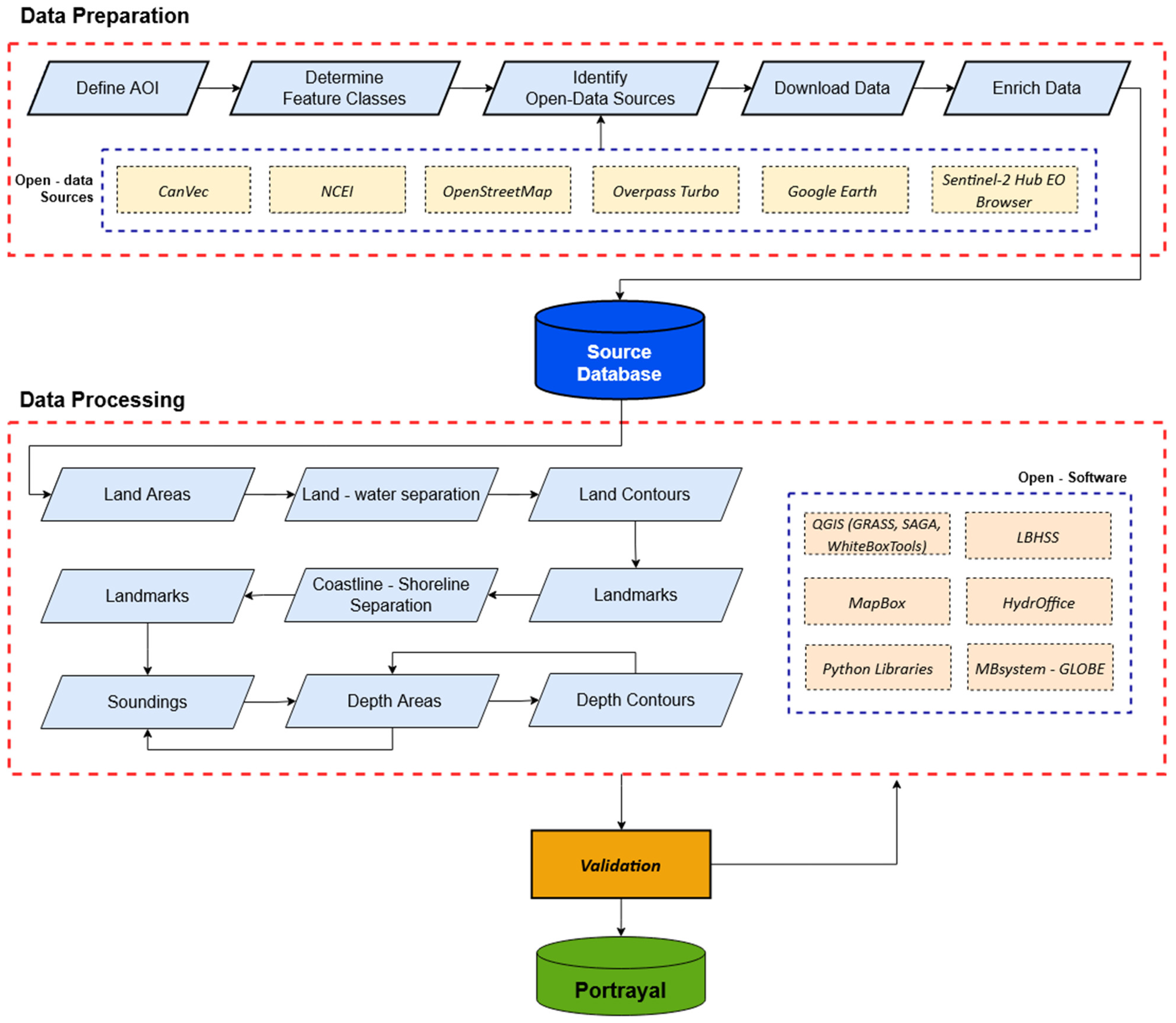
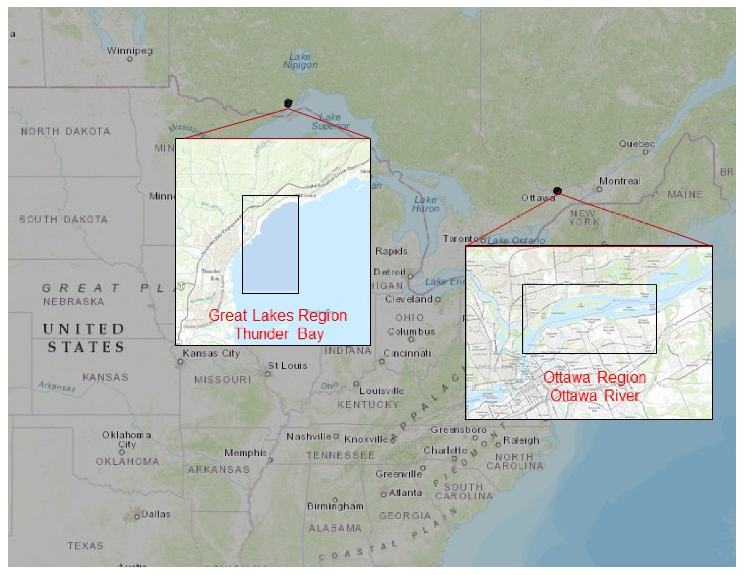
2. Methodology
2.1. Data Preparation
2.2. Data Processing
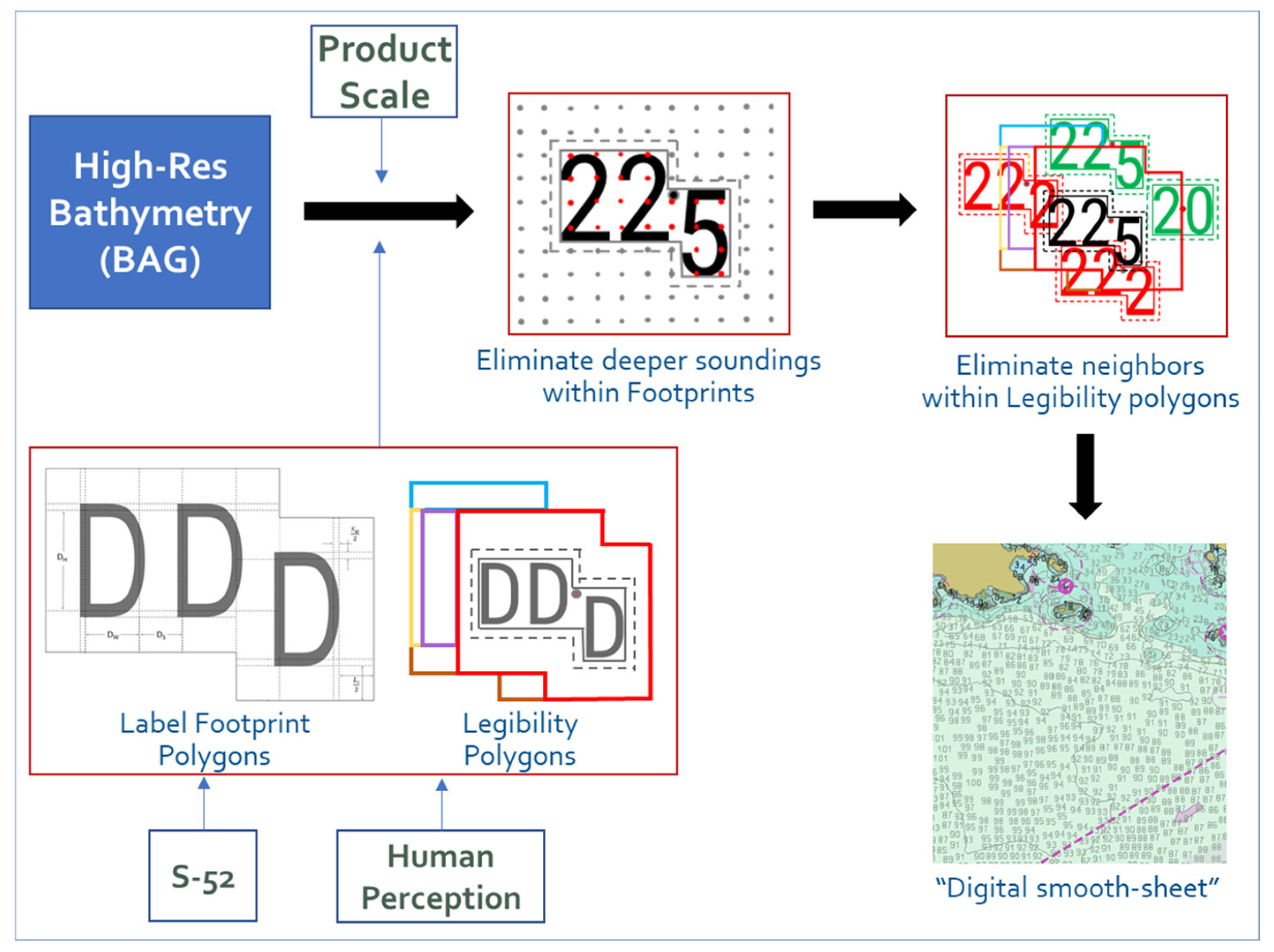
- Least Depth: the shallowest sounding of a seafloor feature, e.g., the pinnacle of a seamount, dome, or ridge, delineated by a depth contour.
- Shoal: the shallowest local sounding representing the depth over an isolated shoal, which may or may not be delineated by a depth contour. A least depth is always a shoal, but not vice versa; the location is the determining factor.
- Deep: the deepest local sounding, e.g., a depression.
- Supportive: soundings that portray additional information about the seafloor morphology, e.g., changes in slope away from least depth, shoal, and deep soundings.
- Fill: soundings used to estimate depths between widely spaced depth contours.
2.3. Data Portrayal
3. Results
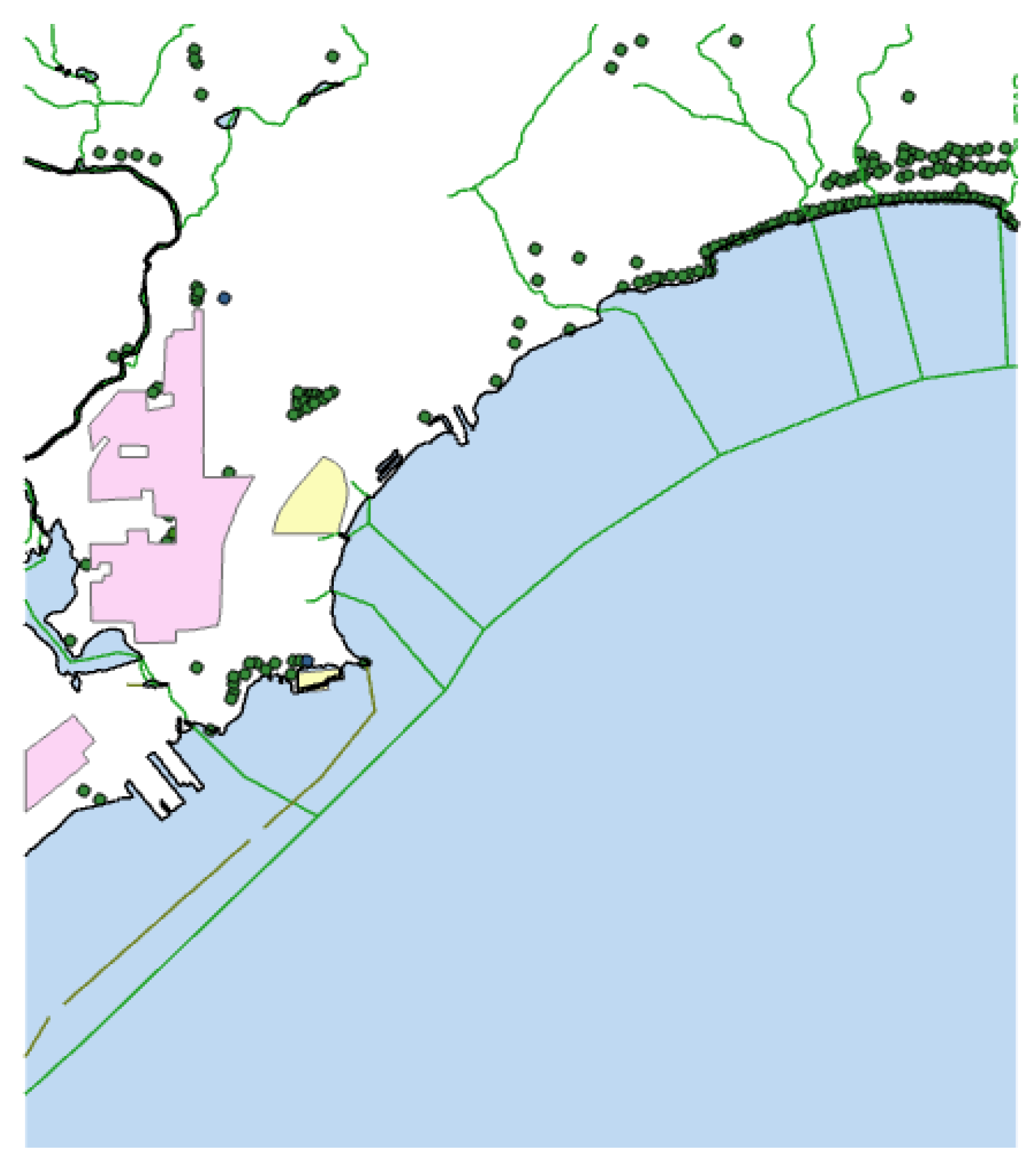
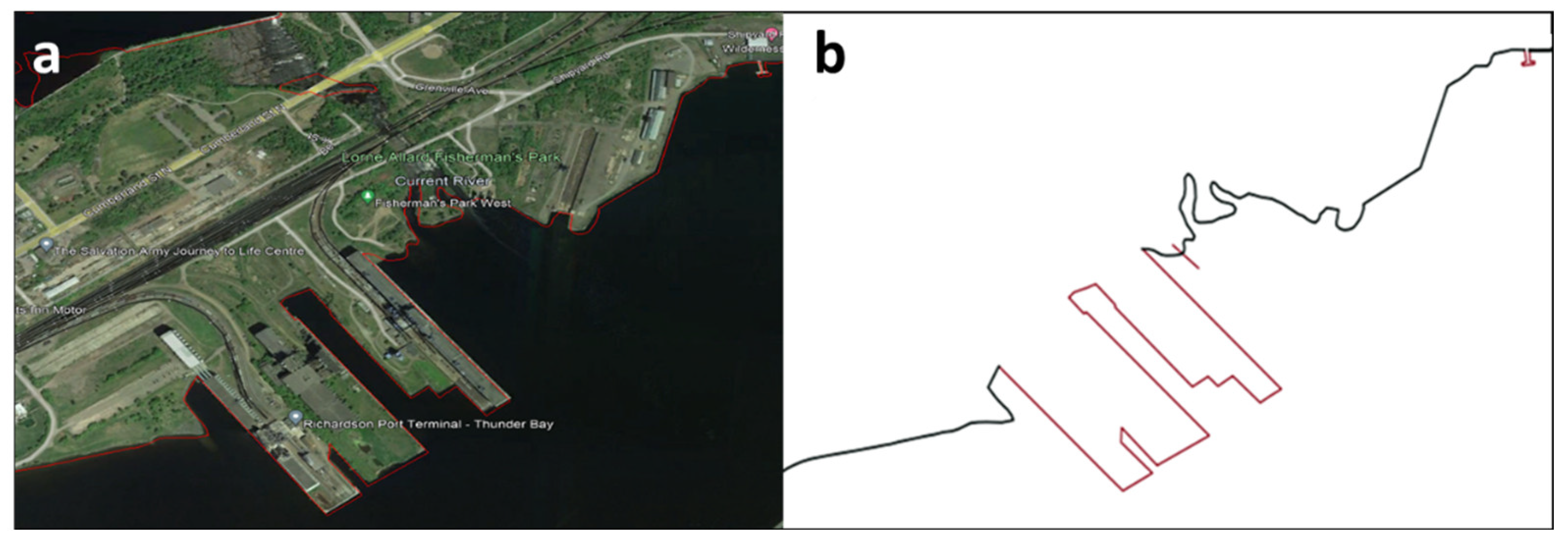
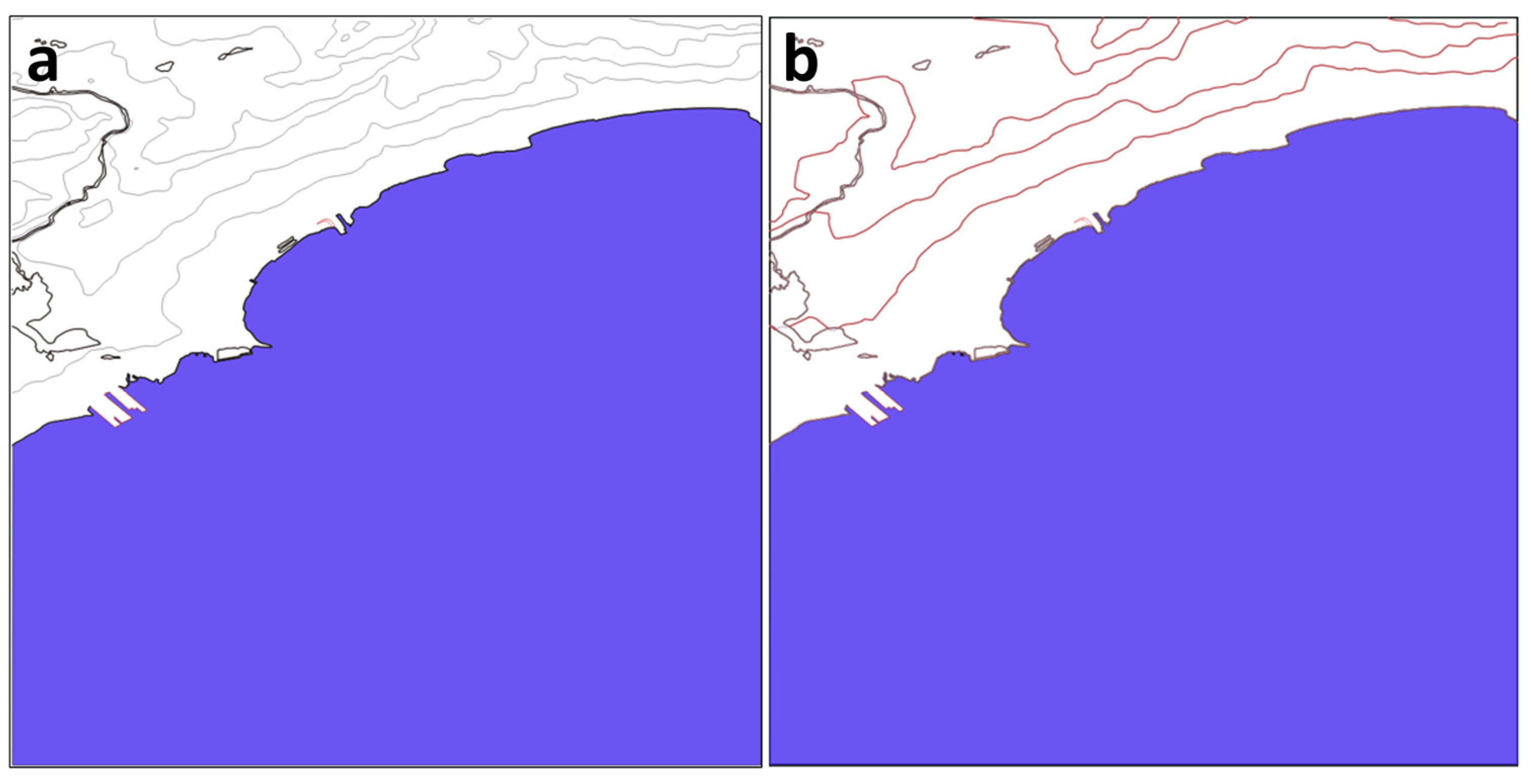
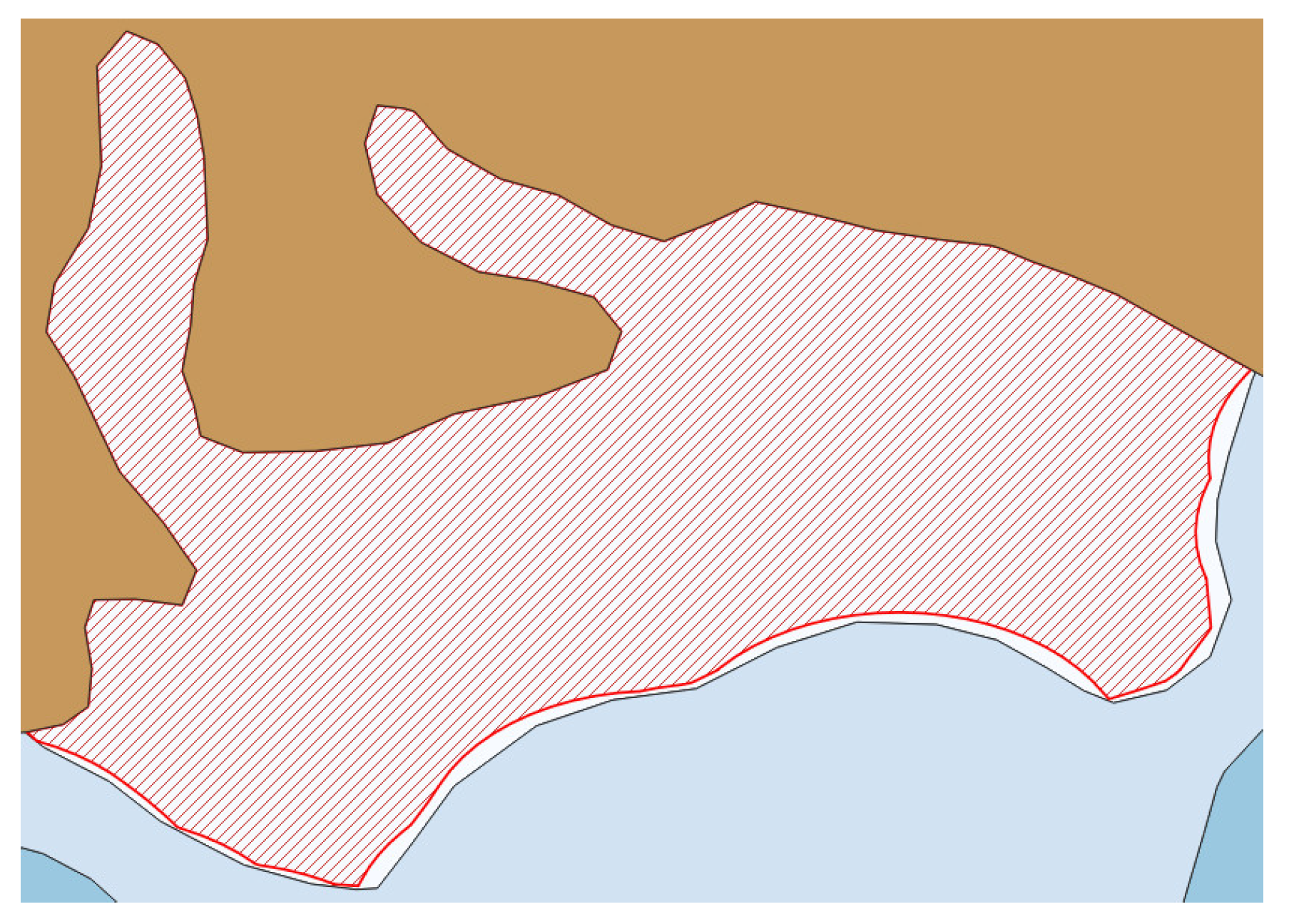
3.1. Compilation of Land Features
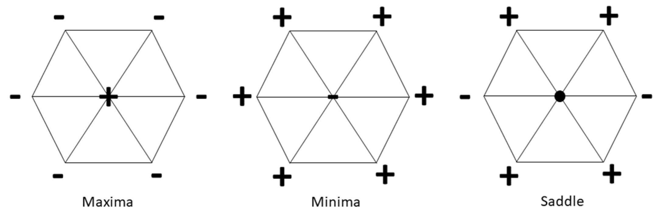
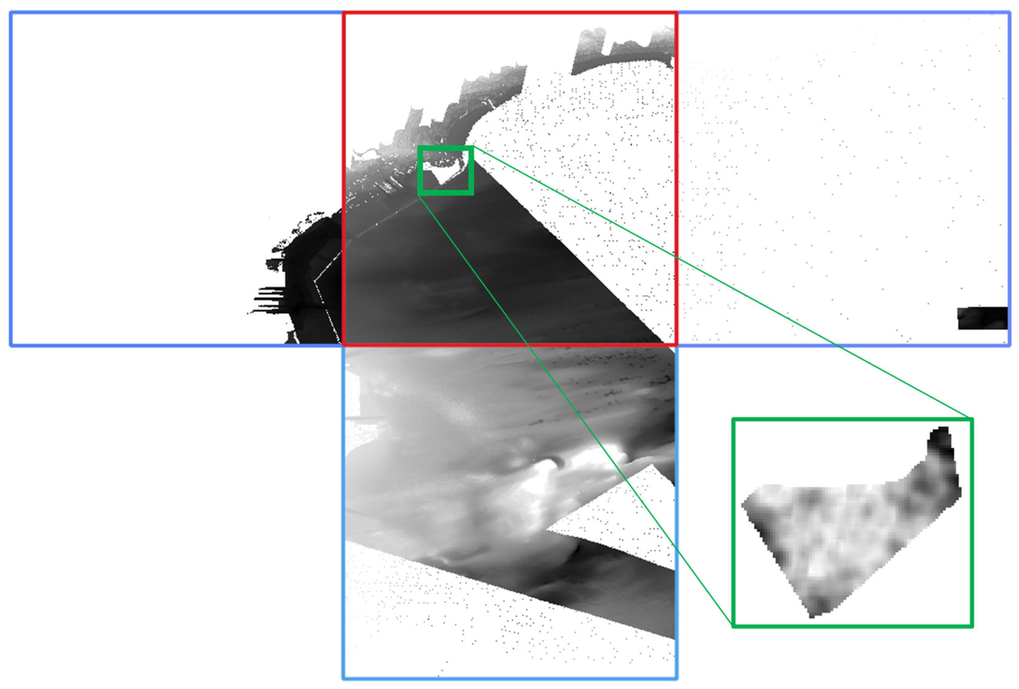
3.2. Compilation of Bathymetric Features
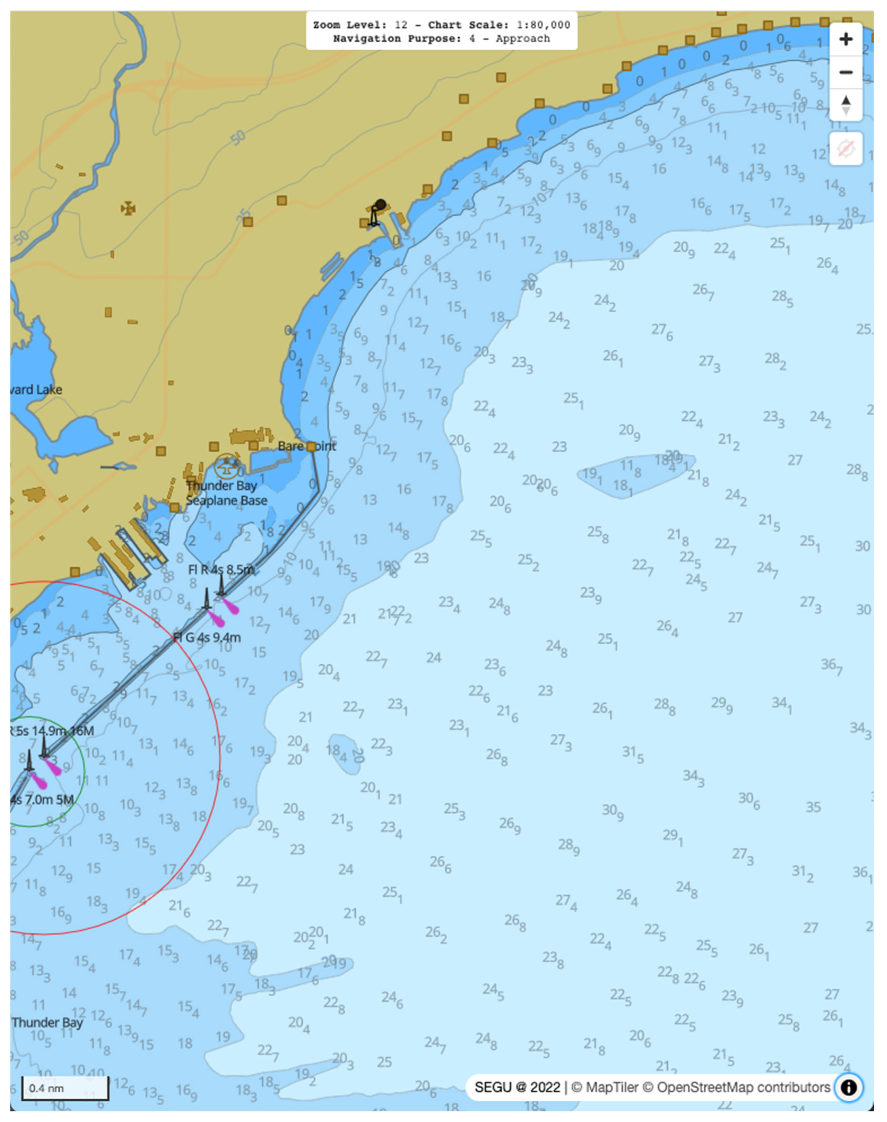
3.3. Mapping Products
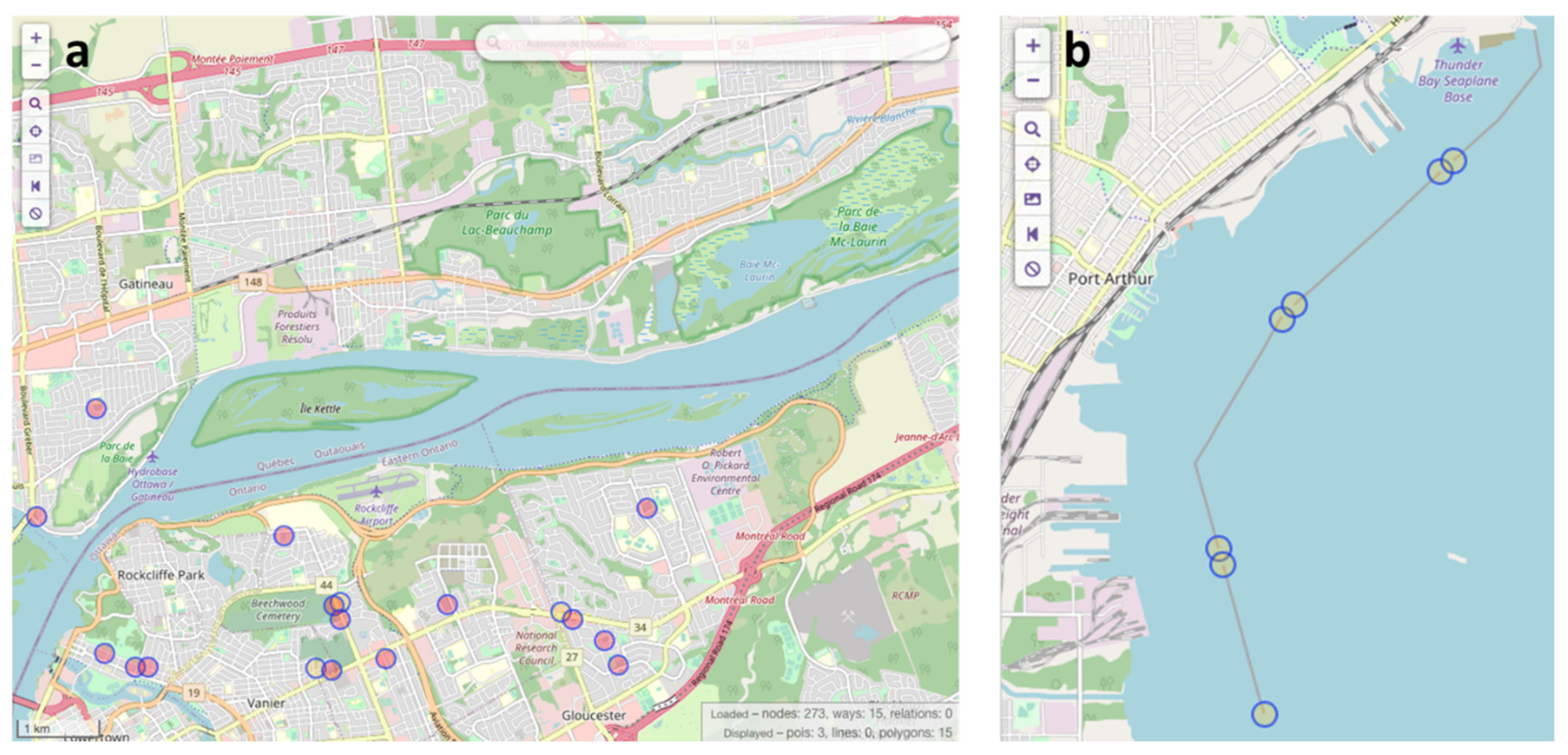
3.4. Evaluation
4. Concluding Remarks
Author Contributions
Funding
Data Availability Statement
Acknowledgments
Conflicts of Interest
References
- Kastrisios, C.; Pilikou, M. Nautical Cartography Competences and Their Effect to the Realisation of a Worldwide Electronic Navigational Charts Database, the Performance of ECDIS and the Fulfilment of IMO Chart Carriage Requirement. Mar. Policy 2017, 75, 29–37. [Google Scholar] [CrossRef]
- IMO. Adoption of Amendments to the International Convention for the Safety of Life at Sea (SOLAS), 1974, as Amended; Revision to Chapter V—Safety of Navigation, IMO Resolution MSC.99(73); IMO Resolution MSC.99(73); IMO—The International Maritime Organization: London, UK, 2000. [Google Scholar]
- IMO. Adoption of the Revised Performance Standards for Electronic Chart Display and Information Systems (ECDIS); IMO Resolution MSC.232(82); IMO—The International Maritime Organization: London, UK, 2006. [Google Scholar]
- IHO. Specifications for Chart Content and Display Aspects of ECDIS; Publication S-52; 6.1; International Hydrographic Organization: Monaco, France, 2015. [Google Scholar]
- Peters, R.; Ledoux, H.; Meijers, M. A Voronoi-Based Approach to Generating Depth-Contours for Hydrographic Charts. Mar. Geod. 2014, 37, 145–166. [Google Scholar] [CrossRef] [Green Version]
- Kastrisios, C.; Calder, B.R.; Masetti, G.; Holmberg, P. On the Effective Validation of Charted Soundings and Depth Curves. In Proceedings of the US Hydro, Biloxi, MS, USA, 18–21 March 2019. [Google Scholar]
- Zhang, X.; Guilbert, E. A Multi-Agent System Approach for Feature-Driven Generalization of Isobathymetric Line. In Advances in Cartography and GIScience. Volume 1: Selection from ICC 2011, Paris; Ruas, A., Ed.; Springer: Berlin/Heidelberg, Germany, 2011; pp. 477–495. ISBN 978-3-642-19143-5. [Google Scholar]
- Kastrisios, C.; Ware, C. Textures for Coding Bathymetric Data Quality Sectors on Electronic Navigational Chart Displays: Design and Evaluation. Cartogr. Geogr. Inf. Sci. 2022, 49, 1–20. [Google Scholar] [CrossRef]
- Winn, C. High-Definition Charts Advance Precision Marine Navigation. Available online: https://nauticalcharts.noaa.gov/updates/high-definition-charts-advance-precision-marine-navigation/ (accessed on 19 February 2023).
- Oraas, S.R. Automated Sounding Selection. Int. Hydrogr. Rev. 1975, 52, 103–115. [Google Scholar]
- MacDonald, G. Computer Assisted Sounding Selection Techniques. Int. Hydrogr. Rev. 1984, 61, 93–109. [Google Scholar]
- Lovrinčević, D. Quality Assessment of an Automatic Sounding Selection Process for Navigational Charts. Cartogr. J. 2017, 54, 139–146. [Google Scholar] [CrossRef]
- Skopeliti, A.; Stamou, L.; Tsoulos, L.; Pe’eri, S. Generalization of Soundings across Scales: From DTM to Harbour and Approach Nautical Charts. ISPRS Int. J. Geo-Inf. 2020, 9, 693. [Google Scholar] [CrossRef]
- Li, M.; Zhang, A.; Zhang, D.; Di, M.; Liu, Q. Automatic Sounding Generalization Maintaining the Characteristics of Submarine Topography. IEEE J. Sel. Top. Appl. Earth Obs. Remote Sens. 2021, 14, 10278–10286. [Google Scholar] [CrossRef]
- Dyer, N.; Kastrisios, C.; Floriani, L. De Label-Based Generalization of Bathymetry Data for Hydrographic Sounding Selection. Cartogr. Geogr. Inf. Sci. 2022, 49, 338–353. [Google Scholar] [CrossRef]
- Yu, W. Automatic Sounding Generalization in Nautical Chart Considering Bathymetry Complexity Variations. Mar. Geod. 2018, 41, 68–85. [Google Scholar] [CrossRef]
- Sui, H.; Zhu, X.; Zhang, A. A System for Fast Cartographic Sounding Selection. Mar. Geod. 2005, 28, 159–165. [Google Scholar] [CrossRef]
- Du, J.; Lu, Y.; Zhai, J. A Model of Sounding Generalization Based on Recognition of Terrain Features. In Proceedings of the 20th International Cartographic Conference, Beijing, China, 6–10 August 2001. [Google Scholar]
- Jingsheng, Z.; Yi, L. Recognition and Measurement of Marine Topography for Sounding Generalization in Digital Nautical Chart. Mar. Geod. 2005, 28, 167–174. [Google Scholar] [CrossRef]
- Smith, S.M. The Navigation Surface: A Multipurpose Bathymetric Database; University of New Hampshire: Durham, NH, USA, 2003. [Google Scholar]
- Guilbert, E.; Lin, H. B-Spline Curve Smoothing under Position Constraints for Line Generalisation. In Proceedings of the 14th Annual ACM International Symposium on Advances in Geographic Information Systems, Arlington, VA, USA, 10–14 November 2006; pp. 3–10. [Google Scholar]
- Guilbert, E.; Saux, E. Cartographic Generalisation of Lines Based on a B-spline Snake Model. Int. J. Geogr. Inf. Sci. 2008, 22, 847–870. [Google Scholar] [CrossRef]
- Guilbert, E. Feature-Driven Generalization of Isobaths on Nautical Charts: A Multi-Agent System Approach. Trans. GIS 2016, 20, 126–143. [Google Scholar] [CrossRef] [Green Version]
- Yu, W.; Zhang, Y.; Ai, T.; Chen, Z. An Integrated Method for DEM Simplification with Terrain Structural Features and Smooth Morphology Preserved. Int. J. Geogr. Inf. Sci. 2021, 35, 273–295. [Google Scholar] [CrossRef]
- Miao, D.; Calder, B. Gradual Generalization of Nautical Chart Contours with a Cubic B-Spline Snake Model. In Proceedings of the 2013 OCEANS, San Diego, CA, USA, 23–26 September 2013; pp. 1–7. [Google Scholar]
- Skopeliti, A.; Tsoulos, L.; Pe’eri, S. Depth Contours and Coastline Generalization for Harbour and Approach Nautical Charts. ISPRS Int. J. Geo-Inf. 2021, 10, 197. [Google Scholar] [CrossRef]
- Yang, H.; Li, L.; Hu, H.; Wu, Y.; Xia, H.; Liu, Y.; Tan, S. A Coastline Generalization Method That Considers Buffer Consistency. PLoS ONE 2018, 13, e0206565. [Google Scholar] [CrossRef]
- Cheng, T.; Li, Z. Effect of Generalization on Area Features: A Comparative Study of Two Strategies. Cartogr. J. 2006, 43, 157–170. [Google Scholar] [CrossRef]
- Zhang, L.; Tang, L.; Jia, S.; Dai, Z. A Method for Selecting Islands Automatically Based on Competitive Influence Domains. IOP Conf. Ser. Earth Environ. Sci. 2019, 237, 22002. [Google Scholar] [CrossRef] [Green Version]
- Douglas, D.H.; Peucker, T.K. Algorithms for the Reduction of the Number of Points Required to Represent a Digitized Line or Its Caricature. Cartogr. Int. J. Geogr. Inf. Geovisualization 1973, 10, 112–122. [Google Scholar] [CrossRef] [Green Version]
- Wang, Z.; Müller, J.-C. Line Generalization Based on Analysis of Shape Characteristics. Cartogr. Geogr. Inf. Syst. 1998, 25, 3–15. [Google Scholar] [CrossRef]
- Dyer, N.; Kastrisios, C.; De Floriani, L. Towards an Automated Chart-Ready Cartographic Sounding Selection. In Proceedings of the 2022 Canadian Hydrographic Conference, Gatineau, OT, Canada, 6–9 June 2022. [Google Scholar]
- Socha, W.; Stoter, J. First Attempts to Automatize Generalization of Electronic Navigational Charts—Specifying Requirements and Methods. In Proceedings of the 6th ICA Workshop on Generalization and Map Production, Dresden, Germany, 23–24 August 2013. [Google Scholar]
- Nada, T.; Kastrisios, C.; Calder, B.; Ence, C.; Greene, C.; Bethell, A.; Hosuru, M. The Nautical Cartographic Constraints and an Automated Generalization Model. In Proceedings of the 2022 Canadian Hydrographic Conference, Gatineau, OT, Canada, 6–9 June 2022. [Google Scholar]
- Nada, T.; Kastrisios, C.; Calder, B.R.; Ence, C.; Greene, C.; Bethell, A. Automated Chart Compilation and Verification of Output Topology and Safety. In Proceedings of the 31st International Cartographic Conference, Cape Town, South Africa, 13–18 August 2023. [Google Scholar]
- Lecordix, F.; Le Gallic, J.-M.; Gondol, L.; Braun, A. Development of a New Generalisation Flowline for Topographic Maps. In Proceedings of the 10th ICA Workshop on Generalisation and Multiple Representation, Moscow, Russia, 2–3 August 2007. [Google Scholar]
- Foerster, T.; Stoter, J.; Kraak, M.-J. Challenges for Automated Generalisation at European Mapping Agencies: A Qualitative and Quantitative Analysis. Cartogr. J. 2010, 47, 41–54. [Google Scholar] [CrossRef]
- Revell, P.; Regnauld, N.; Bulbrooke, G. OS Vectormap District: Automated Generalization, Text Placement and Conflation in Support of Making Pubic Data Public. In Proceedings of the 25th International Cartographic Conference, Paris, France, 3–8 July 2011. [Google Scholar]
- Burghardt, D.; Duchêne, C.; Mackaness, W. Conclusion: Major Achievements and Research Challenges in Generalisation. In Abstracting Geographic Information in a Data Rich World; Burghardt, D., Duchêne, C., Mackaness, W., Eds.; Springer: Berlin/Heidelberg, Germany, 2014; ISBN 978-3-319-00202-6. [Google Scholar]
- Stoter, J.; Post, M.; van Altena, V.; Nijhuis, R.; Bruns, B. Fully Automated Generalization of a 1:50k Map from 1:10k Data. Cartogr. Geogr. Inf. Sci. 2014, 41, 1–13. [Google Scholar] [CrossRef]
- United Nations Conference on Trade and Development. Review of Maritime Transport 2022. Navigating Stormy Waters; United Nations: New York, NY, USA, 2022. [Google Scholar]
- Contarinis, S.; Kastrisios, C. Marine Spatial Data Infrastructure. In Geographic Information Science & Technology Body of Knowledge; Wilson, J.P., Ed.; University Consortium for Geographic Information Science: Ithaca, NY, USA, 2022. [Google Scholar] [CrossRef]
- IHO. Spatial Data Infrastructures “The Marine Dimension” Guidance for Hydrographic Offices; Publication C-17; 2.0.0; International Hydrographic Organization: Monaco, France, 2017. [Google Scholar]
- Manyika, J.; Chui, M.; Groves, P.; Farrell, D.; Van Kuiken, S.; Almasi Doshi, E. Open Data: Unlocking Innovation and Performance with Liquid Information; McKinsey Global Institute: Atlanta, GA, USA, 2013. [Google Scholar]
- Contarinis, S.; Nakos, B.; Tsoulos, L.; Palikaris, A. Web-Based Nautical Charts Automated Compilation from Open Hydrospatial Data. J. Navig. 2022, 75, 763–783. [Google Scholar] [CrossRef]
- Contarinis, S.; Kastrisios, C.; Nakos, B. Marine Protected Areas and Electronic Navigational Charts: Legal Foundation, Mapping Methods, IHO S-122 Portrayal, and Advanced Navigation Services. Euro-Mediterr. J. Environ. Integr. 2023. [Google Scholar] [CrossRef]
- Affonso, J.; Kastrisios, C.; Parrish, C.; Calder, B.R. A Geographically Adaptive Model for Satellite Derived Bathymetry. In Proceedings of the 2022 Canadian Hydrographic Conference, Gatineau, OT, Canada, 6–9 June 2022. [Google Scholar]
- Kastrisios, C.; Calder, B.R. Algorithmic Implementation of the Triangle Test for the Validation of Charted Soundings. In Proceedings of the 7th International Conference on Cartography & GIS., Sofia, Bulgaria, 18–23 June 2018; Volume 1, pp. 569–576. [Google Scholar]
- Kastrisios, C.; Calder, B.; Masetti, G.; Holmberg, P. Towards Automated Validation of Charted Soundings: Existing Tests and Limitations. Geo-Spat. Inf. Sci. 2019, 22, 290–303. [Google Scholar] [CrossRef] [Green Version]
- Masetti, G.; Faulkes, T.; Kastrisios, C. Automated Identification of Discrepancies between Nautical Charts and Survey Soundings. ISPRS Int. J. Geo-Inf. 2018, 7, 392. [Google Scholar] [CrossRef] [Green Version]
- Masetti, G.; Faulkes, T.; Kastrisios, C. Hydrographic Survey Validation and Chart Adequacy Assessment Using Automated Solutions. In Proceedings of the US HYDRO 2019, Biloxi, MS, USA, 18–21 March 2019; pp. 1–13. [Google Scholar]
- Kastrisios, C.; Calder, B.R.; Bartlett, M. Inspection and Error Remediation of Bathymetric Relationships of Adjoining Geo-Objects in Electronic Navigational Charts. In Proceedings of the 8th International Conference on Cartography and GIS, Nessebar, Bulgaria, 15–20 June 2020; pp. 116–123. [Google Scholar]
- Cordero, J.; Kastrisios, C. Characterizing Free and Open-Source Tools for Ocean-Mapping. In Proceedings of the 6th Hydrographic Engineering Conference, Lisbon, Portugal, 3–5 November 2020; pp. 53–56. [Google Scholar]
- Cordero, J.; Kastrisios, C. Using Free and Open-Source Software in Ocean Mapping: The Case Study of the Spanish EEZ Project near the Canary Islands. In Proceedings of the US Hydro 2021 Conference, online, 13–16 September 2021. [Google Scholar]
- Kastrisios, C.; Ware, C.; Calder, B.R.; Butkiewicz, T.; Alexander, L.; Broekman, R. Improved Techniques for Depth Quality Information on Navigational Charts. In Proceedings of the 8th International Conference on Cartography & GIS., Nessebar, Bulgaria, 20–25 June 2020; Bandrova, T., Konečný, M., Eds.; Bulgarian Cartorgaphic Association: Nessebar, Bulgaria. [Google Scholar]
- Kastrisios, C.; Ware, C.; Calder, B.; Butkiewicz, T.; Alexander, A.L.; Hauser, O. Nautical Chart Data Uncertainty Visualization as the Means for Integrating Bathymetric, Meteorological, and Oceanographic Information in Support of Coastal Navigation. In Proceedings of the 100th American Meteorological Society Meeting, 18th Symposium on Coastal Environment, Boston, MA, USA, 12–16 January 2020. [Google Scholar]
- Ware, C.; Kastrisios, C. Evaluating Countable Texture Elements to Represent Bathymetric Uncertainty. In Proceedings of the EuroVis 2022—Short Papers; Agus MarcoAigner, W.T., Ed.; The Eurographics Association: Rome, Italy, 2022; pp. 1–55. [Google Scholar]
- Kastrisios, C.; Contarinis, S.; Butkiewicz, T.; Nakos, B.; Sullivan, B.; Harmon, C.; Ence, C.; Bartlett, M. User-Centered Design of Nautical Chart Symbols. In Proceedings of the U.S. Hydro 2023—Hydrospatial: The Next Frontier of Hydrography, Mobile, AL, USA, 13–16 March 2023. [Google Scholar]
- IHO. Transfer Standard for Digital Hydrographic Data; Publication S-57; 3.1; International Hydrographic Organization: Monaco, France, 2000. [Google Scholar]
- Weintrit, A. Clarification, Systematization and General Classification of Electronic Chart Systems and Electronic Navigational Charts Used in Marine Navigation. Part 2—Electronic Navigational Charts. TransNav Int. J. Mar. Navig. Saf. Sea Transp. 2018, 12, 769–780. [Google Scholar] [CrossRef] [Green Version]
- Nyberg, J.; Pe’eri, S.; Catoire, S.; Harmon, C. An Overview of the NOAA ENC Re-Scheaming Plan. Int. Hydrogr. Rev. 2020, 24, 7–20. [Google Scholar]
- IHO. Standards for Hydrographic Surveys, Publication S-44, 5th ed.; International Hydrographic Organization: Monaco, France, 2008. [Google Scholar]
- NOAA Office of Coast Survey ASSIST. Available online: https://www.nauticalcharts.noaa.gov/customer-service/assist/ (accessed on 19 February 2023).
- IHO. Guidance to Crowdsourced Bathymetry; Publication B-12; 3.0.0; International Hydrographic Organization: Monaco, France, 2022. [Google Scholar]
- Calder, B. Design of a Wireless, Inexpensive Ocean of Things System for Volunteer Bathymetry. IEEE Internet Things J. 2023, 1. [Google Scholar] [CrossRef]
- Manzano, L.J. The bathymetric compilation, a true challenge in the nautical chart generation process. Int. Hydrogr. Rev. 2021, 25, 55–75. [Google Scholar]
- NOAA National Centers for Environmental Information. Available online: https://www.ncei.noaa.gov/ (accessed on 4 January 2023).
- USGS Earth Explorer. Available online: https://earthexplorer.usgs.gov/ (accessed on 4 January 2023).
- Natural Resources Canada Topographic Data of Canada—CanVec Series. Available online: https://open.canada.ca/data/en/dataset/8ba2aa2a-7bb9-4448-b4d7-f164409fe056 (accessed on 4 January 2023).
- Government of Canada Geospatial Data Extraction. Available online: https://maps.canada.ca/czs/index-en.html (accessed on 5 January 2023).
- Lyzenga, D.R. Passive Remote Sensing Techniques for Map- Ping Water Depth and Bottom Features. Appl. Opt. 1978, 17, 379–383. [Google Scholar] [CrossRef]
- Philpot, W.D. Bathymetric Mapping with Passive Multispectral Imagery. Appl. Opt. 1989, 28, 1569–1578. [Google Scholar] [CrossRef]
- Su, H.; Liu, H.; Heyman, W.D. Automated Derivation of Bathymetric Information from Multi-Spectral Satellite Imagery Using a Non-Linear Inversion Model. Mar. Geod. 2008, 31, 281–298. [Google Scholar] [CrossRef]
- Dierssen, H.M.; Zimmerman, R.C.; Leathers, R.A.; Downes, T.V.; Davis, C.O. Ocean Color Remote Sensing of Seagrass and Bathymetry in the Bahamas Banks by High-Resolution Airborne Imagery. Limnol. Oceanogr. 2003, 48, 444–455. [Google Scholar] [CrossRef]
- Stumpf, R.P.; Holderied, K.; Sinclair, M. Determination of Water Depth with High-Resolution Satellite Imagery over Variable Bottom Types. Limnol. Oceanogr. 2003, 48, 547–556. [Google Scholar] [CrossRef]
- NOAA Nautical Chart Manual. Volume 1—Policies and Procedures; Version 2022.2; U.S. Department of Commerce, Office of Coast Survey: Silver Spring, MD, USA, 2022. [Google Scholar]
- IHO. Regulations of the IHO for International (INT) Charts and Chart Specifications of the IHO; Publication S-4; 4.9.0; International Hydrographic Organization: Monaco, France, 2021. [Google Scholar]
- IHO. IHO Transfer Standard for Digital Hydrographic Data; Supplementary Information for the Encoding of S-57 Edition 3.1 ENC Data. S-57 Supplement No. 3; Publication S-57; 3.1.3; International Hydrographic Organization: Monaco, France, 2014. [Google Scholar]
- IHO. IHO Electronic Navigational Chart Product Specification; Publication S-101; 1.0.0; International Hydrorgaphic Organization: Monaco, France, 2018. [Google Scholar]
- Owens, E.; Brennan, R.T. Methods To Influence Precise Automated Sounding Selection via Sounding Attribution & Depth Areas. In Proceedings of the Canadian Hydrographic Conference 2012, Niagara Falls, ON, Canada, 15–17 May 2012. [Google Scholar]
- Kastrisios, C.; Calder, B.R.; Masetti, G.; Martinez, B.; Holmberg, P. Soundings Validation Toolbox: Research to Operations. In Proceedings of the 2020 Canadian Hydrographic Conference, Quebec City, Canada, 24–27 February 2020. [Google Scholar]
- Lorensen, W.E.; Cline, H.E. Marching Cubes: A High Resolution 3D Surface Construction Algorithm. SIGGRAPH Comput. Graph. 1987, 21, 163–169. [Google Scholar] [CrossRef]
- IHO. ENC Validation Checks; Publication S-58; 6.1.0.; International Hydrographic Organization: Monaco, France, 2018. [Google Scholar]
- Yao, X.A. Spatial Queries. In Geographic Information Science & Technology Body of Knowledge; Wilson, J.P., Ed.; University Consortium for Geographic Information Science: Ithaca, NY, USA, 2021; Volume 2021. [Google Scholar]
- Caress, D.W.; Chayes, D.N. MB-Systems. Available online: www.mbari.org/products/researchsoftware/mb-system (accessed on 15 February 2023).
- Wintersteller, P.; Foskolos, N.; Ferreira, C.; Karantzalos, K.; Lampridou, D.; Baika, K.; Anbar, J.; Quintana, J.; Kokorotsikos, S.; Pisa, C.; et al. The NEANIAS Project—Bathymetric Mapping and Processing Goes Cloud; MARUM: Bremen, Germany, 2021. [Google Scholar] [CrossRef]
- Poncelet, C.; Billant, G.; Corre, M.-P. Globe (GLobal Oceanographic Bathymetry Explorer) Software; SEANOE, 2022. [Google Scholar]
- QGIS.org. QGIS Geographic Information System. QGIS Association. Available online: http://www.qgis.org (accessed on 15 February 2023).
- Lindsay, J. The Whitebox Geospatial Analysis Tools Project and Open-Access GIS. In Proceedings of the GIS Research UK 22nd Annual Conference, Glasgow, Scotland, 16–18 April 2014; pp. 16–18. [Google Scholar]
- Neteler, M.; Mitasova, H. Open Source GIS.; Springer: Boston, MA, USA, 2002; ISBN 978-1-4757-3580-2. [Google Scholar]
- Conrad, O.; Bechtel, B.; Bock, M.; Dietrich, H.; Fischer, E.; Gerlitz, L.; Wehberg, J.; Wichmann, V.; Böhner, J. System for Automated Geoscientific Analyses (SAGA) v. 2.1.4. Geosci. Model Dev. 2015, 8, 1991–2007. [Google Scholar] [CrossRef] [Green Version]
- Wilson, M.; Masetti, G.; Calder, B.R. Automated Tools to Improve the Ping-to-Chart Workflow. Int. Hydrogr. Rev. 2017, 17, 21–30. [Google Scholar]
- Van Rossum, G.; Drake, F.L. Python Reference Manual; Centrum voor Wiskunde en Informatica: Amsterdam, The Netherlands, 1995. [Google Scholar]
- IHO. Annex A: Data Classification and Encoding Guide; Publication S-101; 1.1.0.; International Hydrographic Organization: Monaco, France, 2020. [Google Scholar]
- IHO-IOC. The IHO-IOC GEBCO Cook Book; Publication B-11; International Hydrographic Organization, Intergovernmental Oceanographic Commission: Monaco, France, 2019. [Google Scholar]
- CHC. The Speed Mapping Challenge—From Data to Chart. Canadian Hydrographic Conference. Available online: https://chc2022.org/en/speed-mapping-challenge-data-chart (accessed on 15 February 2023).


| ENC Code | Description | Geometric Primitive | Display Order |
|---|---|---|---|
| LNDARE | Land Area | Polygon | 1 |
| DEPARE | Depth Area | Polygon | 2 |
| LAKARE | Lakes Area | Polygon | 3 |
| UNSARE | Unsurveyed Area | Polygon | 4 |
| BUISGL_POLY | Buildings | Polygon | 5 |
| M_COVR | Chart Coverage | Line | 6 |
| Highways | Line | 7 | |
| Aeroways | Line | 8 | |
| COALNE | Coastline | Line | 9 |
| DEPCNT | Depth Contours | Line | 10 |
| LNDCNT | Land Contours | Line | 11 |
| SLCONS | Shoreline Constructions | Line | 12 |
| SOUNDG | Soundings | Point | 13 |
| LIGHTS | Lighthouses | Point | 14 |
| BUISGL | Buildings | Point | 15 |
| CHIMNY | Chimneys | Point | 16 |
| AIRPRT | Airports | Point | 17 |
| POSGEN | Elevation Positions | Point | 18 |
| SILBUI | Silo | Point | 19 |
| BUIREL | Places of Worship | Point | 20 |
| NAME | POIs | Point | 21 |
| ISLAND | Islands | Point | 22 |
| Site | Lat | Long | Datum Separation |
|---|---|---|---|
| Great Lakes Region—Thunder Bay | 48.4° | 89.2° | IGLD85 is 183.20 m below CD HWL is 0.93 M above CD |
| 48.5° | 89.2° | ||
| 48.4° | 89.1° | ||
| 48.5° | 89.1° | ||
| Ottawa Region—Ottawa River | 45.44° | 75.7° | ICGVD-2013 is 40.53 m below CD HWL is 2.44 M above CD |
| 45.48° | 75.7° | ||
| 45.44° | 75.6° | ||
| 45.48° | 75.6° |
Disclaimer/Publisher’s Note: The statements, opinions and data contained in all publications are solely those of the individual author(s) and contributor(s) and not of MDPI and/or the editor(s). MDPI and/or the editor(s) disclaim responsibility for any injury to people or property resulting from any ideas, methods, instructions or products referred to in the content. |
© 2023 by the authors. Licensee MDPI, Basel, Switzerland. This article is an open access article distributed under the terms and conditions of the Creative Commons Attribution (CC BY) license (https://creativecommons.org/licenses/by/4.0/).
Share and Cite
Kastrisios, C.; Dyer, N.; Nada, T.; Contarinis, S.; Cordero, J. Increasing Efficiency of Nautical Chart Production and Accessibility to Marine Environment Data through an Open-Science Compilation Workflow. ISPRS Int. J. Geo-Inf. 2023, 12, 116. https://doi.org/10.3390/ijgi12030116
Kastrisios C, Dyer N, Nada T, Contarinis S, Cordero J. Increasing Efficiency of Nautical Chart Production and Accessibility to Marine Environment Data through an Open-Science Compilation Workflow. ISPRS International Journal of Geo-Information. 2023; 12(3):116. https://doi.org/10.3390/ijgi12030116
Chicago/Turabian StyleKastrisios, Christos, Noel Dyer, Tamer Nada, Stilianos Contarinis, and Jose Cordero. 2023. "Increasing Efficiency of Nautical Chart Production and Accessibility to Marine Environment Data through an Open-Science Compilation Workflow" ISPRS International Journal of Geo-Information 12, no. 3: 116. https://doi.org/10.3390/ijgi12030116