Article

Spatial Non-Stationarity of Influencing Factors of China’s County Economic Development Base on a Multiscale Geographically Weighted Regression Model

1
School of Geography and Remote Sensing, Guangzhou University, Guangzhou 510006, China
2
School of Geography and Planning, Sun Yat-Sen University, Guangzhou 510006, China
3
Guangdong Centre for Marine Development Research, Guangzhou 510220, China
4
Guangzhou Urban Planning and Design Survey Research Institute, Guangzhou 510030, China
5
Guangdong Enterprise Key Laboratory for Urban Sensing, Monitoring and Early Warning, Guangzhou 510060, China
*
Author to whom correspondence should be addressed.
ISPRS Int. J. Geo-Inf. 2023, 12(3), 109; https://doi.org/10.3390/ijgi12030109
Submission received: 3 February 2023 / Revised: 24 February 2023 / Accepted: 2 March 2023 / Published: 4 March 2023

Abstract

:
The development of the county economy in China is a complicated process that is influenced by many factors in different ways. This study is based on multi-source big data, such as Tencent user density (TUD) data and point of interest (POI) data, to calculate the different influencing factors, and employed a multiscale geographically weighted regression (MGWR) model to explore their spatial non-stationarity impact on China’s county economic development. The results showed that the multi-source big data can be useful to calculate the influencing factor of China’s county economy because they have a significant correlation with county GDP and have a good models fitting performance. Besides, the MGWR model had prominent advantages over the ordinary least squares (OLS) and geographically weighted regression (GWR) models because it could provide covariate-specific optimized bandwidths to incorporate the spatial scale effect of the independent variables. Moreover, the effects of various factors on the development of the county economy in China exhibited obvious spatial non-stationarity. In particular, the Yangtze River Delta, the Pearl River Delta, and the Beijing-Tianjin-Hebei urban agglomerations showed different characteristics. The findings revealed in this study can furnish a scientific foundation for future regional economic planning in China.

1. Introduction

The unbalanced distribution of economic activities is the normal state of regional economic development. Revealing the influencing factors of economic development is one of the research hotspots of regional economics [1]. Since the implementation of the reform and opening policy in 1978, China has experienced rapid economic growth and the disparity in economic development between various regions within the country has become increasingly evident [2]. Some studies have demonstrated that different regions of China present different characteristics of economic development [1,3]. Many studies have been carried out to explore the factors which affect economic development in China. For example, Xie (2013) described the spatial distribution characteristics of 108 counties’ economies in the Shandong province of China and summarized that industrialization, government investment, and farmers’ economic level are the main factors influencing a county’s economic growth in Shandong [4]. Sun (2018) found that economic and environmental governance factors as well as population and resource factors are two main elements that restrict the development of a green economy in the Jiangsu province of China [5]. However, these relevant studies are mainly based on using statistical data to explore the influencing factors of China’s economy. The major problem with traditional statistical data is that it is usually produced by census and sampling surveys, which have the limitations of a long production cycle and a lack of timeliness [6]. In addition, the factors affecting economic development are very complex and diverse [7], while the types of statistical data are usually limited, which makes it difficult to obtain information about some variables related to economic development, especially at the county level.
With the progress of society and technology, data types with social perception functions have emerged. Point of interest (POI) data, a kind of social perception big data containing spatial location information, has been proven to be able to be used for economic evaluation [8,9]. Besides, the popularity of the Internet and the wide application of smartphones have led to the rise of another kind of big data with a social perception function, location-based social media (LBSM) data, which has been widely used in studying human activities [10,11] and economic modeling [12,13]. These kinds of big data provide an effective way to obtain information on economic factors. For example, Li (2021) used POI data as the representative of economic activities to understand the pattern and mechanism of Wuhan city spatial agglomeration [14]. Niu (2020) used social media data and remote sensing images to represent the characteristics of social conditions and the built environment respectively, and to produce the indicators of physical, economic, and living conditions that are closely related to poverty in Guangzhou [6]. However, these relevant studies mainly take a certain small region of China as the study area to explore the regional economic development factors, which have strong local economic development characteristics and lack universal applicability [15,16]. At present, a study with the whole county area of China as the research area, combined with multi-source big data to explore the influencing factors of economic development is still relatively lacking.
A variety of mathematical statistics or index methods such as the Malmquist–Luenberger index model [17], linear weighted composite Index model [18], and ordinary regression model [19,20] have been used to examine the correlation between economic development and its driving factors. The assumption in these methods is that the correlation between the independent and dependent variables remains a stable and consistent state in the whole spatial research area [21]. The relations between the independent variables and the dependent variable may exhibit significant spatial variation, which means that one factor affecting economic development in one region may have a completely different impact in other regions [22]. This variation is referred to as spatial non-stationarity, which is difficult to discover in an estimation of the global parameters [23]. The geographically weighted regression (GWR) model, which can acquire each spatial unit’s regression coefficients by borrowing non-parametric estimation from the geographical data of different spatial units, solves the spatial non-stationarity of different variables [24]. In recent years, many studies have used the GWR model to explore the influence of different factors on the economy in space [25,26]. However, in the process of GWR modeling, the same bandwidth is applied to all independent variables, disregarding the scale effect of these variables on the dependent variable. Generally, the emergence of a social and economic phenomenon is frequently shaped by multiple spatial processes of varying scales, and using the GWR model to explore the influencing factors of China’s economy could easily cause deviation [27]. The multiscale geographically weighted regression (MGWR) method, proposed by Fotheringham in 2017, can effectively solve the scale issue of influencing factors [28]. Further, Yu (2019) supplemented and refined the statistical inference of the MGWR model in 2019, so that the MGWR model can be widely used in empirical studies [29]. At present, many studies have used the MGWR model to explore the influencing factors and the spatial effect on different fields, such as air quality [30], distribution of researchers [31], traffic fatalities [32], hukou transfer intentions [33], land transfer [34], and so on. However, this model has rarely been applied in the economy, especially in exploring the influencing factors and their spatial non-stationarity effects on China’s county economic development.
In recent years, China has increased its focus on the imbalance of small regional economic growth and has put forward some policies such as targeted poverty alleviation and rural revitalization to solve this issue. The coordination and mutual development of counties plays a crucial role in advancing regional economic growth [35]. However, the impact mechanism of China’s overall economic development at the county level is still unclear. Understanding the spatial characteristics and key influencing factors of economic development at the county level of China as a whole can help local governments to formulate plans to adapt to the local economic development situation [36]. It is an important link to promote China’s overall economic development coordinately and to narrow the economic gap between rich and poor in the future. Therefore, the objective of this study is to explore the spatial non-stationarity of the influencing factors of China’s county economic development and to analyze the impact of different factors on various regions. Firstly, multi-source big data, such as Tencent user density (TUD) data and point of interest (POI) data, were applied, instead of the traditional economic statistics data, to extract the influencing factors of China’s counties’ economic development, which provides a new variable calculation idea for the analysis of the influential factors of the economy in large regions and at a small scale. Secondly, the MGWR model was compared with the ordinary least squares regression model (OLS) and the GWR model in county economic modeling and was used to understand the spatial non-stationarity of the factors affecting economic development, enriching the application field of the MGWR model. Further, major influencing factors governing the development of the county economy in different regions of China were discussed. This study may strengthen the understanding of the main factors affecting economic development in China at the county level, and provide some scientific reference for future regional development planning.

2. Materials and Methods
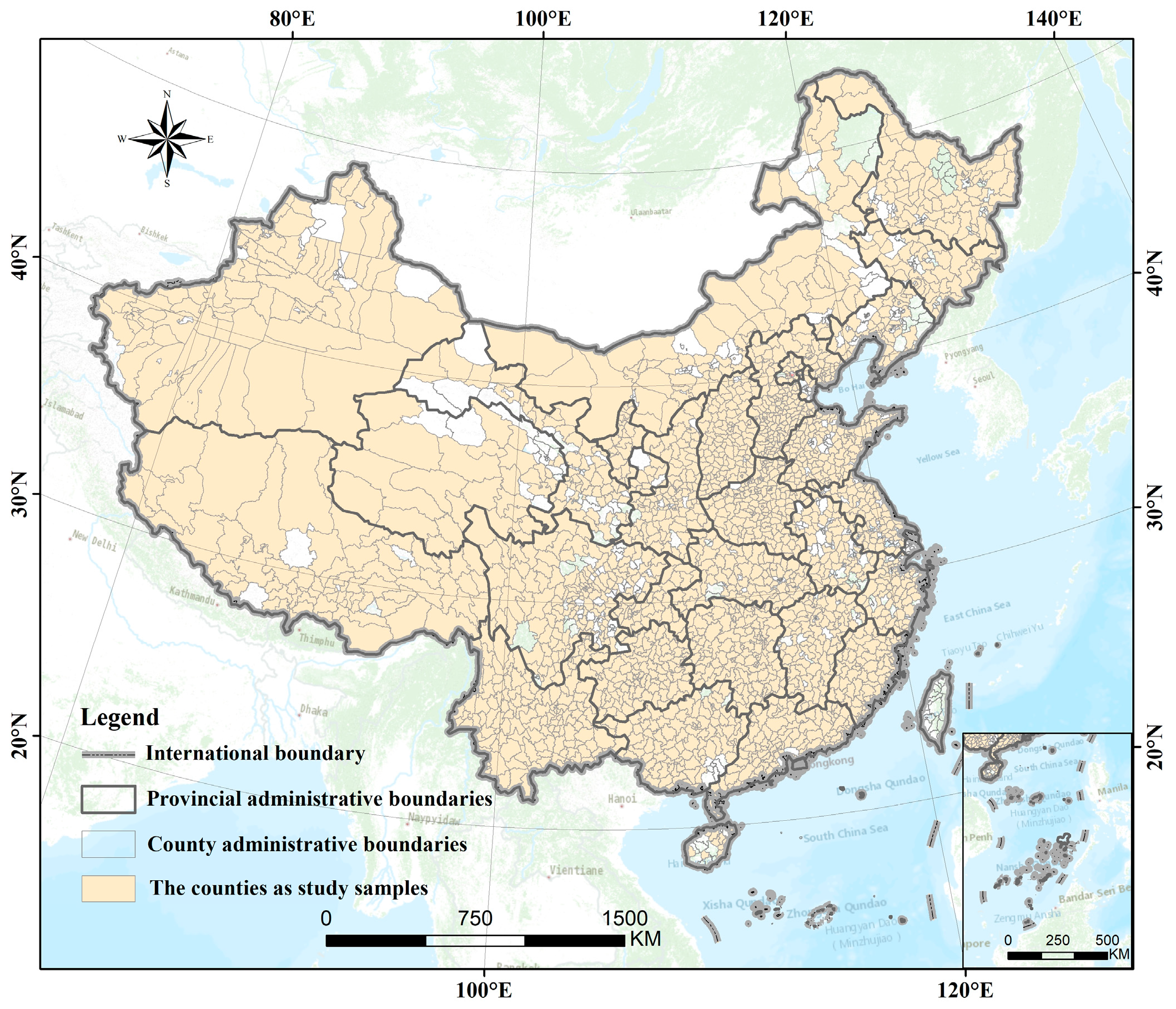
2.1. Study Area

China’s administrative regions are primarily segmented into three levels, including provinces, cities, and counties. This study focused on economic development at the county level. Therefore, 2339 of China’s counties were selected as the sample to explore the influencing factors of China’s county economic development and the spatial differentiation characteristics. The county-level regions in China mainly include four types: county, flag, county-level city, and municipal district, which were treated as equivalent statistical units in this study. The study areas are shown in Figure 1.

2.2. Variables Selection and Processing

The dependent variable in this study was the Gross Domestic Product (GDP), which was used to represent the economic development of counties in China. The county-level GDP data were collected from the 2020 Statistical Yearbook of Chinese counties. In addition, multi-source big data was used in this study to extract the independent variables as the influencing factors of economic development. Considering that economic development is affected by various factors, this study divided all influencing factors into five categories: natural factors, social media factors, business factors, infrastructure factors, and land-use factors.

2.2.1. Natural Factors

By using a geographical detector, Wang and Peng (2021) have found that the topographical and climatic factors have a positive correlation with other economic dominant factors, which can augment their effect on GDP density [16]. Digital Elevation Model (DEM) has usually been used to represent topographic change [8]. Therefore, this study collected DEM data with 500 m resolution from the Resources and Environment Science and Data Center. In addition, the rainfall data of meteorological stations in China were collected from the National Meteorological Science Data Center, and Kriging spatial interpolation was carried out to obtain the 500 m resolution annual average rainfall data for China in 2019. These data were reprojected to the Lambert projection, and then the average altitude (ALT) and average annual rainfall (RAIN) of each county in China were obtained by combining the county administrative boundary data in China based on the zonal statistic tool in ArcGIS 10.2.

2.2.2. Social Media Factors

The widespread utilization of smartphones has led to social media data becoming a commonly used data source to reflect social and economic activities and human behavior. Tencent location big data is a typical type of social media data that records the position information of Tencent application users on mobile terminal equipment and has wide coverage in China [37,38]. A recent study has highlighted the potential of Tencent user density (TUD) data in assessing China’s county-level economic development due to its high positioning accuracy and advantages in reflecting both daytime and nighttime human activities [13]. Referring to Huang’s (2021) processing of Tencent location big data [13], this study stimulated the annual TUD data from 2019 and then calculated the total TUD at the county level based on the zonal statistic tool in ArcGIS 10.2 as the social media factor to explore the impact of Chinese social media users’ vitality on county economic development.

2.2.3. Business Factors

Relevant studies have proven that business can improve the local economy and job creation, which makes a positive contribution to social economic well-being [39,40,41]. At the same time, points of interest (POI), a kind of geospatial big data with geographic locations and textual descriptions of the category, can effectively distinguish industrial and commercial areas and can provide the distribution information of different types of business, such as a corporation, factory, real estate industry, leisure industry, and so on [42]. Thus, this study obtained the different types of POI data in 2017 from the Baidu map open platform and then used the kernel density analysis tool in ArcGIS 10.2 to calculate different types of POI density data. The parameter settings for kernel density estimation are 500 m pixel size and 1 km search radius, which are consistent with the parameters of TUD data processing. Finally, combined with county administrative boundary data, the different types of POI density data were summarized by using the zonal statistic tool in ArcGIS 10.2 to obtain the variables of corporation business (CORP), realty business (REALTY), and entertainment business (ENT) as the business factors in this study. Among these, CORP mainly contains the density information for the pharmaceutical industry, network technology, the advertising industry, metallurgy, the chemical industry, commercial trade, and various types of limited companies; REALTY includes the density information for buildings closely related to the realty industry, such as residential communities, villas, dormitories, and other premises; while ENT contains the density information for scenic spots, cultural squares, exhibitions, games halls, karaoke bars, gymnasiums, and other leisure entertainment venues.

2.2.4. Infrastructure Factors

Previous studies have found that transportation and public facilities have a great impact on regions’ economic growth [43,44]. According to the relevant findings, road traffic data from 2020 obtained from the AMAP open platform and POI data in 2017 from Baidu map open platform for public service facilities were used to calculate the road traffic (ROAD) and public service facilities (PUB) variables, respectively, as the infrastructure factors in this study. Among these, ROAD contains the density information for roads above the national level, and PUB contains the density information for public toilets, newsstands, emergency shelters, and other public service places. The data processing of infrastructure factors is the same as for the business factors.

2.2.5. Land Use Factors

Reasonable and intensive land use is important for sustainable economic development [45]. A relevant study has demonstrated that the development of construction land could affect regional investment, which can further affect local economic growth [46]. This study first resampled the 1 km resolution land used to generate data from 2019 obtained from the Resources and Environment Science and Data Center at 500 m resolution. Then the total arable land area (ALAND) and the total construction land area (CLAND) for each county were calculated as the land-use factors to explore the influence of land-use status on county economic development.
Before modeling, to facilitate the comparison and weighting of variables of different units, this study used the SPSS Statistics 26 software to conduct z-score standardization processing for all variables, removing the unit limitation of data. The detailed descriptions and the correlations with GDP of the different independent variables are summarized in Table 1. The Pearson correlation coefficients (PCC) show that the independent variables selected in this study have a significant correlation with county GDP at level 0.01. In addition, the Variance Inflation Factor (VIF) values of each independent variable are less than 10, which means that there is no collinearity problem between the variables when building models.

2.3. Methods

2.3.1. Geographically Weighted Regression (GWR) Model

The GWR model is a local regression model that improves on the traditional global ordinary least squares (OLS) regression model. An important advantage of the GWR model compared to the OLS model is its ability to capture the spatial variation in the relationships between the dependent variable and the independent variables [47,48,49]. The equation for the GWR model is shown as follows:
y i = β 0 ( u i , v i ) + j = 1 n β j ( u i , v i ) x i j + ε i
where ( u i , v i ) represents the spatial centroid coordinates of county i; y i is the dependent variable value at position i; β 0 ( u i , v i ) is the estimated intercept coefficient at the position ( u i , v i ) ; x i j is the value of the jth independent variable at position i; β j ( u i , v i ) is the jth local regression coefficient for the jth independent variable at the location ( u i , v i ) ; and ε i is the random error associated with location i.
The GWR model assigns higher weights to sample points close to the regression point based on a weight matrix calculated by using a kernel function [47]. This study adopted the bi-square kernel function to calculate the weighted matrix:
w i j = { [ 1 ( d i j b ) 2 ] 2       i f   | d i j | < b 0                               o t h e r w i s e
where w i j is the weight between county i and county j, | d i j | is the distance between count i and county j, and b is the bandwidth determined by minimizing the corrected Akaike information criterion (AICc) [50].
However, the GWR model uses an average of the different bandwidths of each independent variable as the final bandwidth, which means that all variables finally use uniform bandwidth in the model. Consequently, some variables may inaccurately assign larger bandwidths despite having smaller actual bandwidths, while others with greater actual bandwidths may receive smaller assigned bandwidths, resulting in bias and noise in the model [31].

2.3.2. Multiscale Geographically Weighted Regression (MGWR) Model

The MGWR model is an improvement on the GWR model. It considers the scale effects of different variables and adjusts the bandwidth of different variables adaptably, allowing different independent variables to possess different bandwidths [33,51]. The equation for the MGWR model is shown as follows:
y i = β b w 0 ( u i ,     v i ) + j = 1 k β b w j ( u i ,     v i ) x i j + ε i
where ( u i , v i ) represents the spatial centroid coordinates of county i; y i is the dependent variable value at position I; x i j is the value of the j t independent variable at position I; β b w 0 ( u i , v i ) is the estimated intercept coefficient at the position ( u i ,   v i ) ; b w j represents the specific optimal bandwidth used for the calibration of the j conditional relationship; β b w j represents the coefficients of j independent variable with b w bandwidth; and ε i is the random error. Each regression coefficient, β b w j , of the MGWR model is obtained based on local regression, and the bandwidths of each variable are different.
In this study, the MGWR model calculates the weight matrix based on the adaptive bi-square and selects the bandwidth based on AICc. Furthermore, a back-fitting algorithm was used for the model calibration, which is based on generalized additive model (GAM) fitting techniques. The basic idea of back-fitting is to calibrate each term of the model using a smoother under the assumption that all the other terms are known [28]. This study selected the GWR model as the initial estimation. After the initialization settings are determined, the difference between the predicted value obtained from the initial estimation and the real value can be calculated, which is the initial residual ε   ^ :
ε ^ = y j = 1 k f j ^         ( f j = β b w j x j )
The GWR model was used to regress the sum of residuals ( ε ^   ) and the first additive term (   f 1   ^ ) on the first variable ( x 1 ) to find an optimalandwidth ( b w 1 ) and new parameter estimates, which then replace the first additive term (   f 1   ^ ) and residuals (   ε ^ ), and so on, repeating the step until the calculation of the last argument variable ( x k ) is completed and the last additive term ( f k   ^ ) and residuals ( ε ^ ) are updated. The above calculation steps are the first-round iteration and the iterations would continue until the estimate converges to the convergence criteria [29]. This study used SOC-f as the convergence criteria:
S O C f = j = 1 p i = 1 n ( f ^ i j n e w f ^ i j o l d ) 2 n i = 1 n ( j = 1 p f ^ i j n e w ) 2
S O C f has the advantage of emphasizing the relative changes of the additive terms rather than the overall fit of the model, making it a more stringent criterion compared to SOC-RSS [28]. In this study, when the change degree of the estimated regression coefficient was less than 1 × 10⁻⁵, the model fitting was considered complete.
This study built the MGWR model based on the MGWR 2.2 desktop application software developed by Oshan et al. (2019) [51], to further explore the spatial non-stationarity of the influences of different factors on China’s county economic development.

3. Results and Discussion

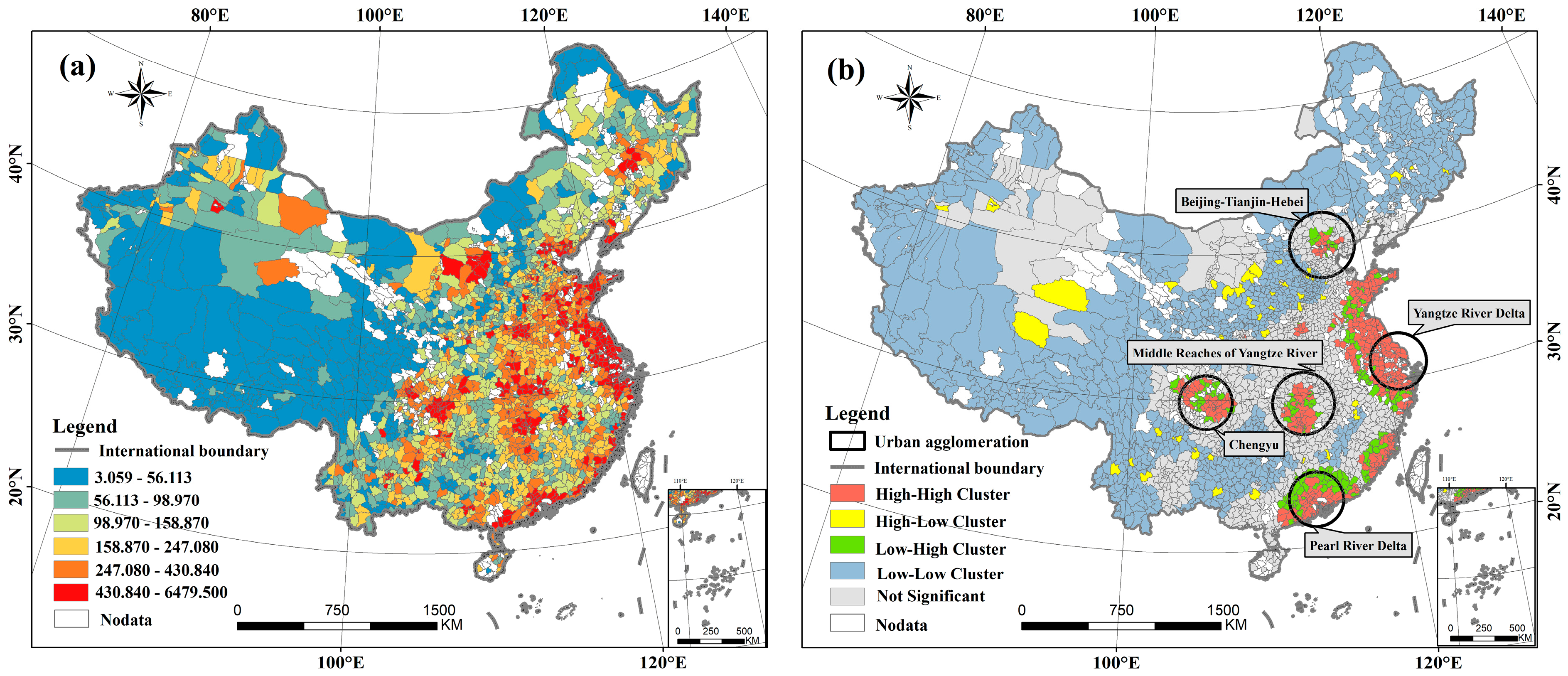
3.1. Spatial Pattern of GDP in China

The distribution of county-level GDP in China is shown in Figure 2a. The economic situation of different regions of China shows significant diversity. Most of the counties with high GDP values are located in the southeast regions and coastal areas of China, while most of the economically underdeveloped counties are concentrated in the northwest regions of China. This study used global Moran’s I to test for the spatial auto-correlation of county-level GDP across China and the p-value, as well as the z-score, were used to measure the significance and reliability of results [52]. The global Moran’s I index is 0.205, which is greater than 0, indicating that China’s county economic development has positive spatial auto-correlation. In addition, the p-value is 0.000, which is less than 0.001, and the z-score is 79.266, which is much higher than 2.58, showing the high significance and reliability of the results.
The local Moran’s I tool, which can reflect the GDP spatial correlation characteristics of each county, is shown in Figure 2b. The counties of the high-high (HH) cluster are mainly located in the economically developed regions of China, such as Beijing-Tianjin-Hebei, the Yangtze River Delta, the middle reaches of the Yangtze River, the Pearl River Delta, and the Chengyu urban agglomerations. Conversely, the counties belonging to the low-low (LL) cluster are mainly concentrated in the western and northern regions, which are the less developed area of China. The high-low (HL) cluster covers a small area and distributes near some LL cluster counties dispersedly. The low-high (LH) clusters are mainly distributed around the HH cluster, which infers that a large gap between the rich and poor exists in those regions. These findings mean that there are significant differences in the spatial distribution of China’s county economy, indicating that it is necessary to examine the factors affecting the spatial distributions of GDP.

3.2. Spatial Variation of Factors Influencing County-Level GDP

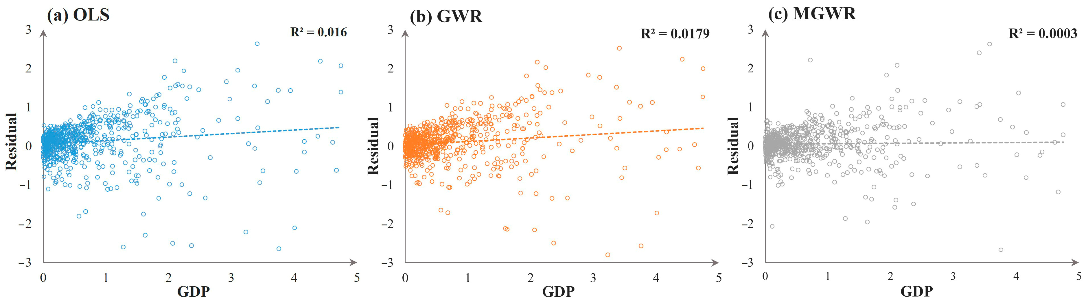
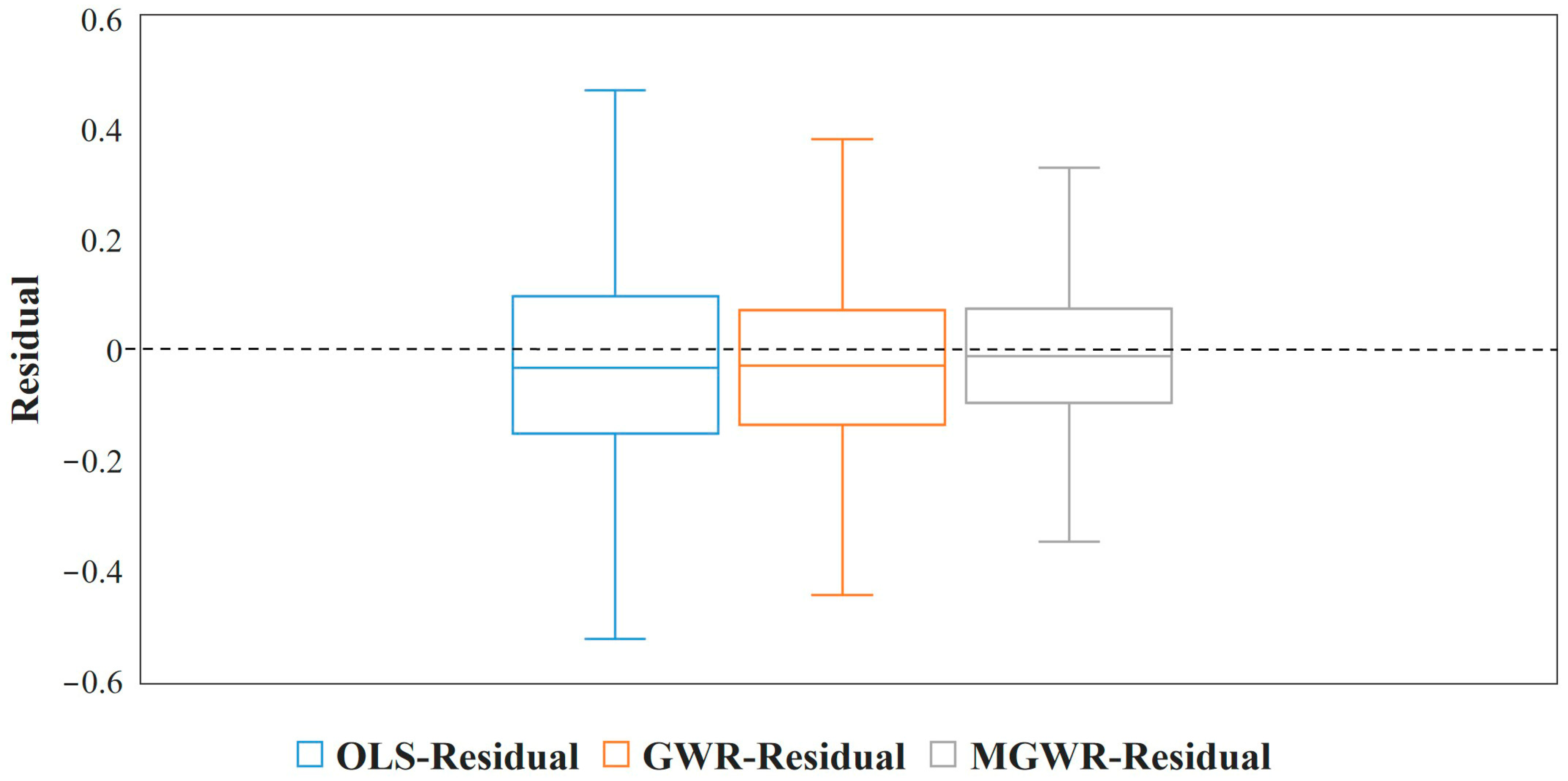
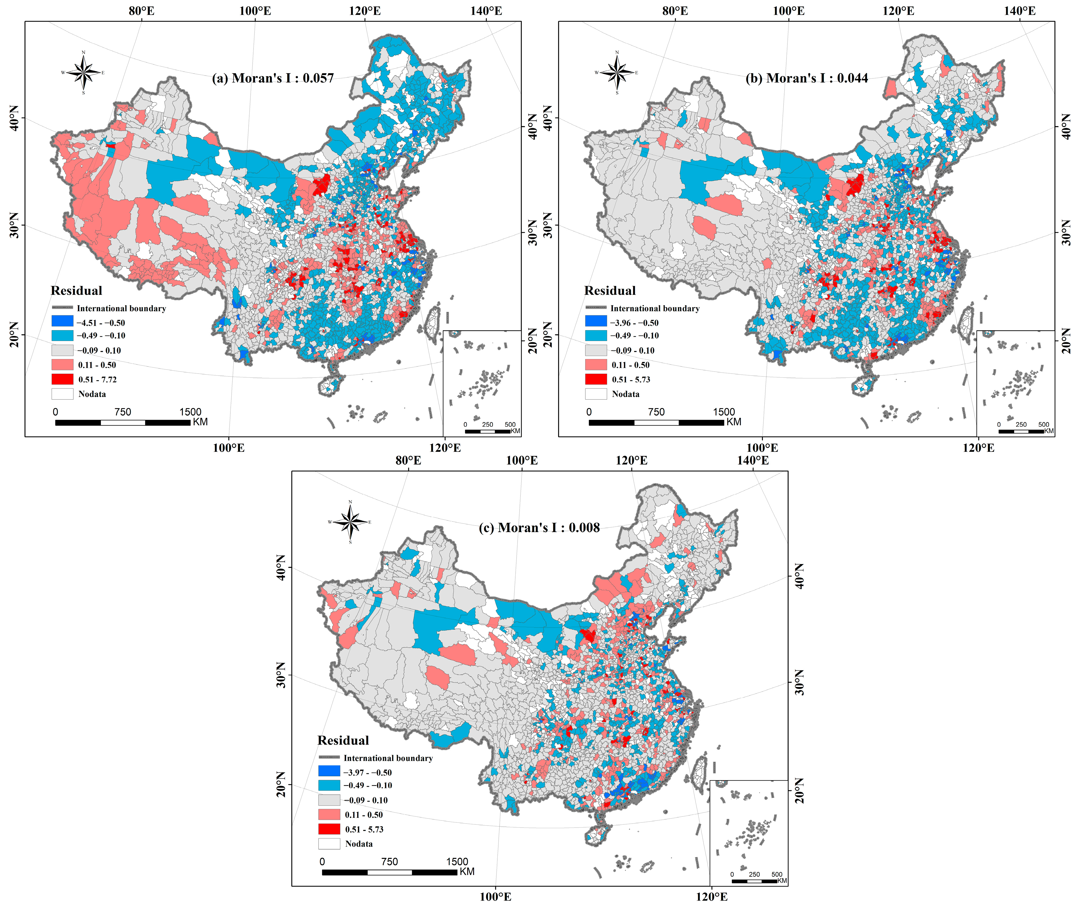
3.2.1. Model Comparison between OLS, GWR, and MGWR

County economic development in China has significantly positive spatial auto-correlation and shows obvious spatial clustering. Therefore, it is necessary to use spatial regression models, such as GWR and MGWR models, to further explore the spatial impact of independent variables on GDP. The performance of OLS, GWR, and MGWR models in China’s county economic modeling was compared in this study.
Firstly, the coefficient, the adjusted R-squared (Adj.R2), the AICc, and the residual sum of squares (RSS) were applied to compare the goodness-of-fit results of the models. As shown in Table 2, the OLS model has the highest value of AICc and the lowest value of Adj.R2, while the MGWR model shows the lowest value of AICc and the highest value of Adj.R2. This indicates that the MGWR model has the best model-fitting capacity which can provide more specific and reliable information than the GWR and OLS models.
Secondly, a heteroscedasticity test of the three models was carried out using the graphic test method. Figure 3 shows the scatter plot of the residuals and dependent variables (standardized GDP) of the three models. It can be seen that the residuals of the three models have no significant correlation with the dependent variables, and most of the data points are randomly distributed between −2 and 2. The results indicate that there is no obvious heteroscedasticity in the three models. In addition, compared with the OLS and GWR models, the MGWR model has the lowest R2, and the data points are more evenly distributed, as well as more concentrated between −2 and 2, which shows that the MGWR model has the weakest heteroscedasticity.
In addition, a box plot was used to compare the residuals of the three models in this study. As shown in Figure 4, the line in the center of the box is the median of the data, representing the average of the residuals in each model. The top and bottom boundaries of the box are the upper and lower quartiles of the residual, which means a box contains 50 percent of the data. The closer the center line of the box is to the zero value and the smaller the width of the box, that the smaller the residual error of the model, and the more stable the model. Figure 4 shows that the MGWR model produces the lowest residuals, as the line in the center of the box is closer to zero compared to the GWR and OLS models, and the area of the box is the smallest.
Another more important criterion to reflect the performance of the model is the spatial auto-correlation degree of the residuals. Spatial auto-correlation in residuals may lead to endogeneity issues, which negatively impact the accuracy of model estimates [53]. Therefore, a criterion for assessing the performance of a regression model is that the residuals should have random and independent distribution. Figure 5 shows the spatial clustering patterns of the residuals of the three models. The residuals of the OLS model exhibit a clear aggregation pattern, with positive residuals concentrated in central and western regions and negative residuals mostly in the north and south. The residuals of the GWR model are dispersed, but some clustering can still be observed, such as positive residual clusters in the eastern coastal areas and negative residual clusters in the northern regions. Meanwhile the residuals of the MGWR model show the least amount of cluster patterns and there is no obvious large areas of clustering compared to the OLS and GWR models. From Moran’s I index of residuals, the OLS model exhibits the strongest levels of positive auto-correlation. Although the spatial auto-correlation level of residuals is reduced in the GWR model, it still exists significantly. It indicates that though the GWR model does improve the issue of residual spatial auto-correlation found in the OLS model, the limitation of unified bandwidth does not eliminate this problem completely. On the contrary, Moran’s I index of the MGWR model’s residuals is the closest to zero, which indicates that the MGWR model can eliminate residual dependency effectively. Consequently, it can be concluded that the MGWR model shows obvious advantages over the traditional global OLS model and the local GWR model with fixed bandwidth in understanding the spatial non-stationarity of influencing factors of China’s county economic development.

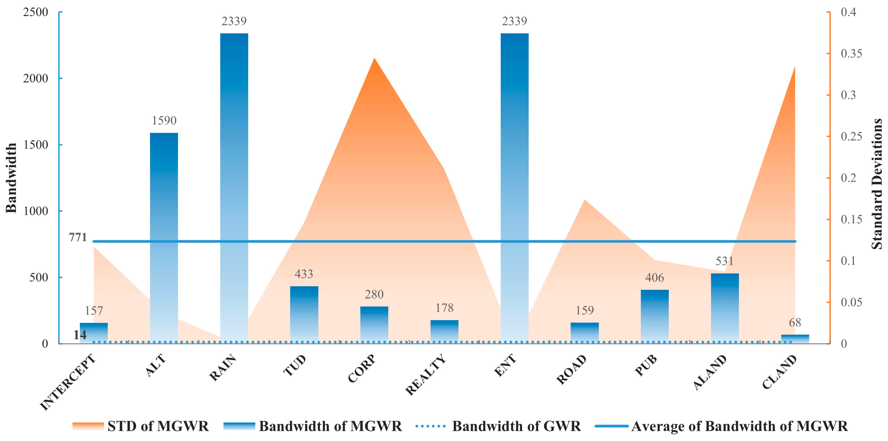
3.2.2. The Spatial Scale Effect regarding Optimized Bandwidths

Generally, the effect of different independent variables on dependent variables varies considerably with changes in the spatial scale. For example, some variables affect the dependent variables in cities, provinces, or at larger spatial scales, while some variables may have a significant influence on counties or at smaller scales. The traditional OLS model ignores the spatial non-stationarity of variables’ impact and the GWR model uses a uniform independent variable bandwidth, which ignores the spatial scale effect of different independent variables. The major advantage of the MGWR model is its ability to not only allow for varying parameter estimates over space, but also generate unique optimal bandwidths for the relationship between the dependent variable and each independent variable, enabling the modeling of various processes’ spatial variation at different scales.
Figure 6 displays the optimal bandwidths for each independent variable generated by the MGWR model as blue histograms. The corresponding standard deviations of the parameter estimates are depicted in the orange areas. The blue dotted line represents the single optimal bandwidth obtained by the GWR model, while the blue solid horizontal line stands for the average of the 11 variables’ bandwidths obtained by the MGWR model. The unified bandwidth of the GWR model (14) is much smaller than the average bandwidths of the MGWR model (771), which indicates that the GWR model and MGWR model differ greatly in the interpretation results of variables. The bandwidths of the individual variables in the MGWR model suggest varying impacts of different independent variables on GDP at different spatial scales. A variable with a large bandwidth influences the dependent variable at a larger spatial scale, while a variable with a small bandwidth affects the dependent variable at a more localized scale. For example, the optimal bandwidths of RAIN and ENT are very large (2339) and are the same as the sample number (2339) of this study, which means that these two are global variables. It indicates that the average annual rainfall and the distribution density of the entertainment industry have similar impacts on economic development nationwide. On the contrary, the bandwidth of CLAND is very small, indicating that the area of construction land affects the economy at local scales, and the parameter estimates have large differences over space. The other variables, such as ROAD, CORP, TUD, and so on, exhibit spatial non-stationarity of the relationship with GDP, and the processes vary at different regional scales because the optimal bandwidth is 157, 280, and 433, respectively. The differences in the influence of independent variables can be reflected by the MGWR model, while it is difficult for them to be reflected by the GWR model. Thus, the MGWR model holds advantages in comprehending the spatial non-stationarity of various factors affecting economic development in China’s counties and in explaining the impact of different independent variables at different spatial scales.

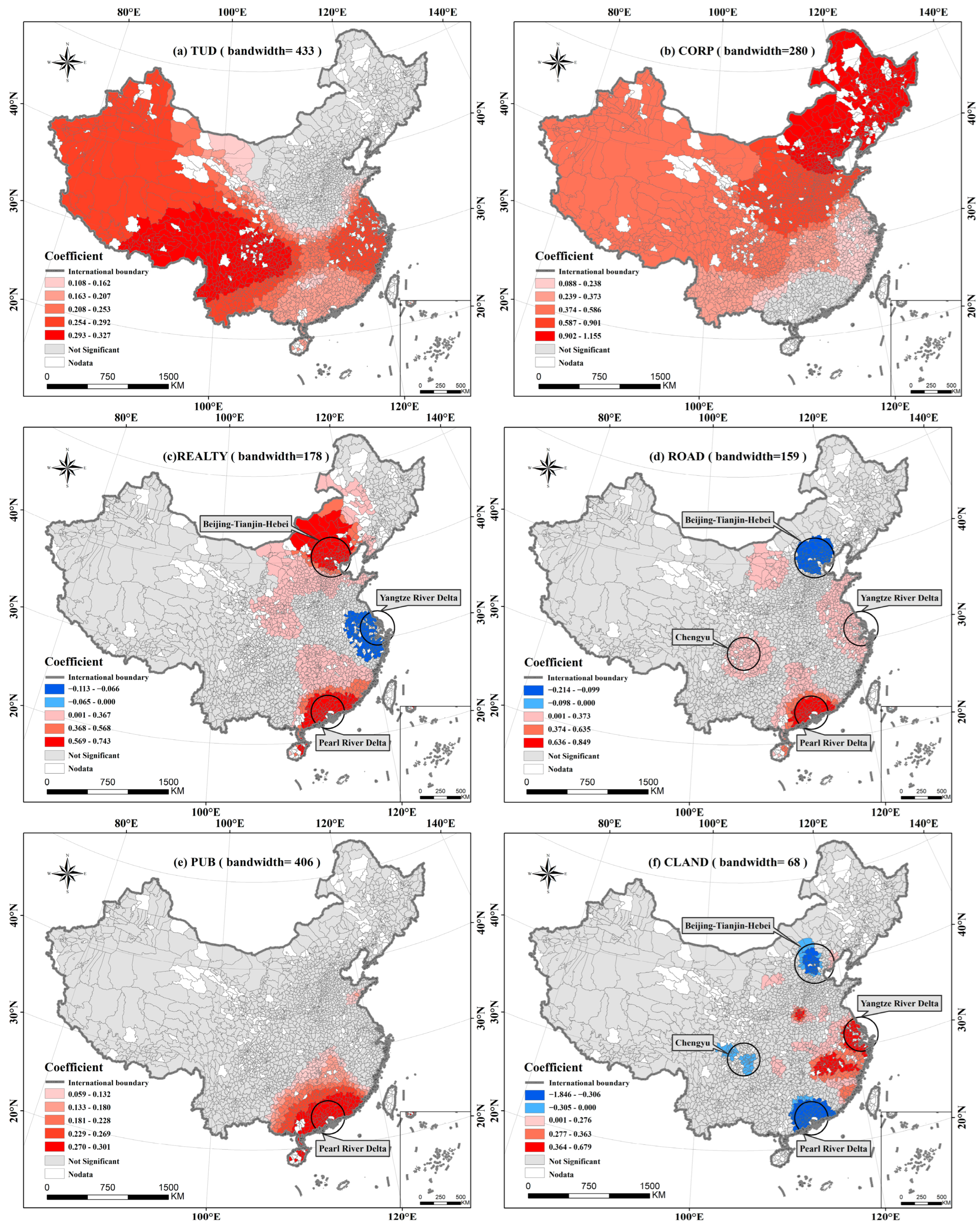
3.2.3. Spatial Variation of Coefficients from the MGWR Model

To enhance our understanding of the impact of various factors on China’s county economic development, this study delves further into the spatial distribution of the local regression coefficients for each independent variable using the MGWR model. Table 3 summarizes the statistics of the different independent variables’ local parameters generated by the MGWR model. The third column of Table 3 shows a classification of coefficients based on t-tests, adjusted for multiple hypothesis testing [54]. It includes the proportion of significant coefficients (p ≤ 0.05), the proportion of significant positive coefficients to significant coefficients (+), and the proportion of significant negative coefficients to significant coefficients (−) [30].
As shown in Table 3, there is the “INTERCEPT” variable, which is the constant term variable. This variable refers to the impact of geographical location change on economic development after all other variables are determined [27]. It shows that geographical location factors have a significant influence on 35.77% of China’s counties. Of these significantly affected counties, 29.39% of them are affected positively, while 70.61% are affected negatively. The local estimates for ALT exhibit a robust and consistent negative relationship with economic development in every county, suggesting that a county’s elevation negatively impacts its economic level. Approximately 88.12% of CORP has a significant positive effect on economic development in China’s counties, indicating that an increase in corporation distribution density is associated with higher economic growth. Similarly, around 62.61% of TUD has a significant positive impact on economic development in China’s counties, indicating that the greater the intensity of social media user activities, the greater the promotion of economic development. The local parameter estimates from REALTY are significant for nearly half of the counties, with most of these counties showing a positive relationship between better realty development and high economic growth, while only 12.33% of the areas are affected negatively. The local parameter estimates from ROAD are significant for one third of the counties, of which 86.51% are affected positively by traffic road density, while 13.49% are affected negatively. The PUB, ALAND, and CLAND variables have a limited impact in a small number of counties, with less than 30% of counties being significantly affected. The local estimates for RAIN and ENT are all insignificant, meaning that these variables have little impact on the economy in China’s counties.
After obtaining the local regression coefficients of different variables based on the MGWR model, six variables—TUD, CORP, REALTY, ROAD, PUB, and CLAND—were mapped in Figure 7, respectively, to reveal the spatial pattern of their influencing effects on the economy. Jenks classification method was used to divide the coefficient of each variable into five grades, in which blue represents a negative influence, red represents a positive influence and gray represents no significant influence.
To begin with, it can be seen from Figure 7a that TUD, a variable reflecting the vitality of Chinese social media users, shows a prominent and positive influence on the economy of most counties of China, especially in the economically backward areas, such as the northwest and southwest of China. The result is consistent with a relevant study which found that TUD has an advantage in reflecting economic development in less developed areas [13]. A recent study has found that the less developed regions of China are facing a situation of low population concentration [55]. This may be because the natural environment, public services, job market, etc. in western China and some less developed areas are not perfect and result in a lower population inflow than in more developed areas [2]. Human beings are the foundation of social development. Therefore, appropriately introducing human capital, increasing population inflow, and social media user vitality in less developed areas can effectively improve economic growth.
Figure 7b displays the spatial pattern of the local coefficient of the CORP variable, which reflects the influence of the distribution density of corporations on GDP. As can be seen, the economy in most counties of China is affected by the density of corporations positively, especially in northeast China, which is the most positively affected area. It indicates that increasing the number of corporations in these areas can better promote economic growth.
As shown in Figure 7c, REALTY, a variable reflecting the intensity of the realty industry, was not significant for most areas of China. This outcome aligns with recent research which discovered weak real estate market investment and no significant contribution to economic development in most regions of China [56]. However, this factor has a significant effect on economic development for the Beijing-Tianjin-Hebei urban agglomeration and its vicinity, as well as the Pearl River Delta urban agglomeration and its surrounding area. This has not been revealed in existing studies.
ROAD was calculated by the traffic road density which can represent the transportation convenience of a region. The local coefficient of ROAD is depicted in its spatial distribution in Figure 7d. It plays a major role in promoting economic development in China, and the counties in the Pearl River Delta are affected by it most significantly. Moreover, some areas of the Yangtze River Delta and Chengyu urban agglomerations are also affected by ROAD positively. It is noteworthy that ROAD does not have a significant positive impact on the economy of the Beijing-Tianjin-Hebei urban agglomeration.
PUB is a variable calculated by the density of public service facilities, which can represent the completeness of regional infrastructure to some extent. It can be seen from Figure 7e that PUB in most regions has no significant influence on economic development, but in south China, especially the Pearl River Delta and its surrounding counties, economic development was positively affected by PUB. A relevant study revealed that the fast pace of urbanization in the southeast coastal regions has led to a large influx of population, causing an imbalance in the supply and demand of public services [57]. Hence, enhancing the allocation of public infrastructure and balancing the supply and demand of public facilities may positively impact the economic development of the Pearl River Delta and surrounding areas.
CLAND represents regional construction land, and the bandwidth of this variable is very small (68), indicating that its influence is in small local regions. As shown in Figure 7f, the GDP of a few counties is significantly affected by CLAND. This is consistent with previous research which found that expanding construction land has made little contribution to economic growth in China [46]. However, this variable has a significant positive impact on the GDP of the Yangtze River Delta urban agglomeration and its surrounding areas, whereas it does not show an obvious positive effect in the Pearl River Delta, Chengyu, and Beijing-Tianjin-Hebei urban agglomerations and their surrounding areas.
This study used multi-source big data to extract the influencing factors of county economic development in China and analyzed the spatial non-stationarity of different factors. Although a relevant study has revealed the important role of producer services (including transportation, the realty industry, commerce, etc.) in China’s economic development, it did not carry out any further comparative analysis on the spatial differences of different industries [41]. With multi-source big data, this study could classify different industries in more detail, and discuss the impact of commerce (CROP), the realty industry (REALTY), and the entertainment industries (ENT) on China’s county economy respectively. At the same time, previous studies have separately discussed the impact of road traffic [43] and construction land on China’s economic development [46]. However, they have only analyzed a small part of China, lacking a comparison of the influence of these variables in different regions of the country. By visualizing the spatial regression coefficients of ROAD and CLAND on the national map, this study found their impacts on different regions in China shows spatial non-stationarity, with particularly significant differences in economic impact on the three major urban agglomerations in China, which has not been revealed by previous studies.

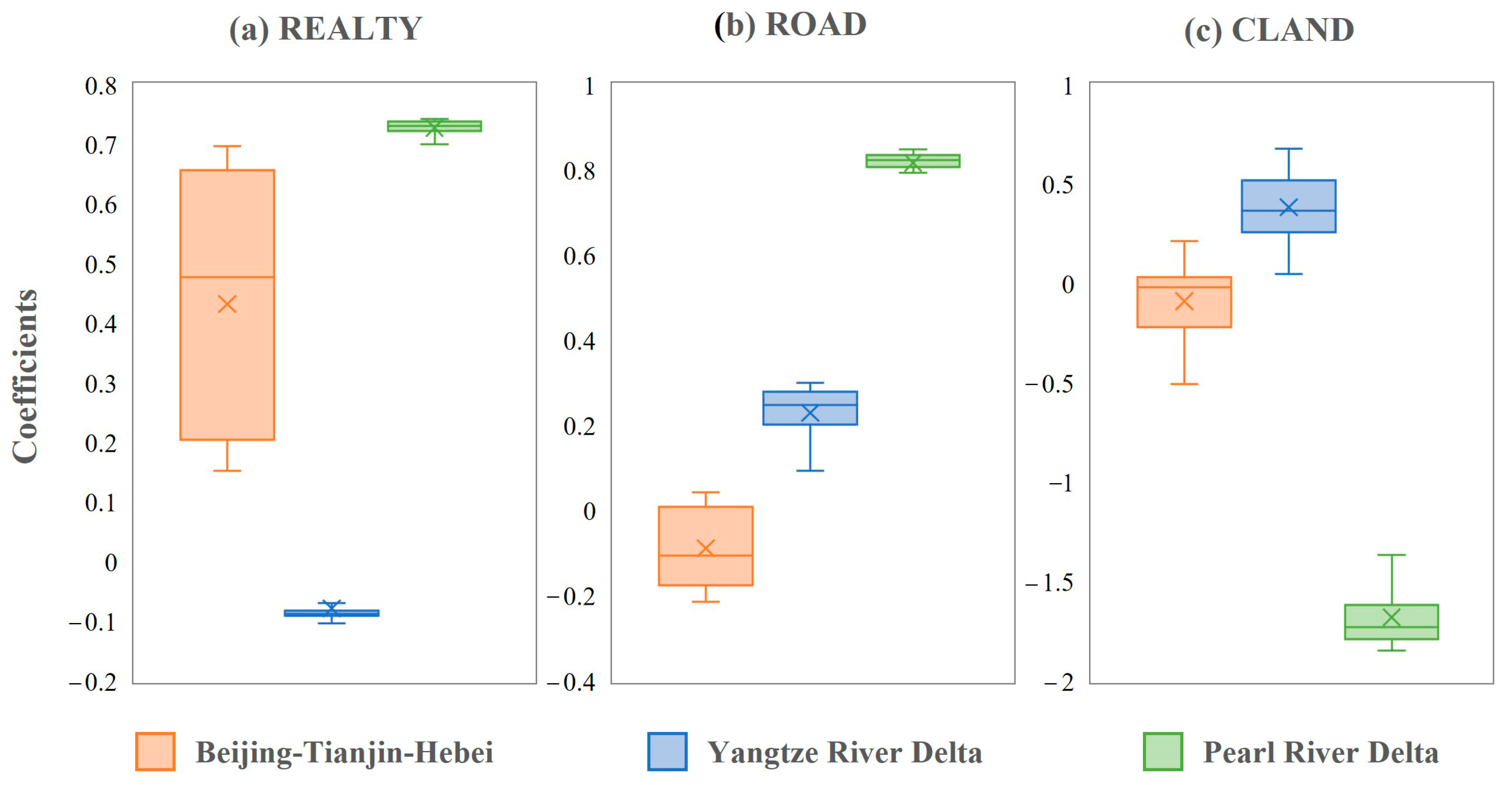
4. Comparison of the Economic Development of Major Urban Agglomerations in China

By using the MGWR model, this study analyzed the impact factors of county economic development in China and discovered that the influence of different factors on county economic development differs across regions in China. In terms of the results shown in Figure 7, the effects of REALTY, ROAD, and CLAND on county GDP are significantly disparate among the Beijing-Tianjin-Hebei, Yangtze River Delta, and Pearl River Delta, which are the three major urban agglomerations in China. Figure 8 further shows the local coefficients of REALTY, ROAD, and CLAND in terms of their impact on the three urban agglomerations’ economic development in China using box plots.
The Beijing-Tianjin-Hebei urban agglomeration contains the capital city of China, which is the economic center of northern China. As shown in Figure 8, the economy of the Beijing-Tianjin-Hebei urban agglomeration is significantly and positively affected by REALTY. At the same time, it is found that there are differences within the Beijing-Tianjin-Hebei region affected by REALTY, for which the spatial regression coefficient values have a large span. This may be related to the differences in real estate development within this region. There are a large number of cities at a lower level of development in the Beijing-Tianjin-Hebei city cluster, and there is a huge development gap between core cities and fringe cities [58]. The core cities, such as Beijing, have more job opportunities but very high housing prices, while the fringe cities have low housing prices but relatively few job opportunities. In order to realize the coordinated development of the economy in the region, the government can strengthen the development of the real estate industry in the region, increasing the supply of housing, and reasonably regulating housing prices. However, the positive impact of ROAD and CLAND on the economy is not significant. It may be because the Beijing-Tianjin-Hebei urban agglomeration is mainly in the radial spatial form, which has relatively developed transportation with its main problem being that there are marginalized nodes [59]. Therefore, the positive impact of ROAD on the economic development of the Beijing-Tianjin-Hebei urban agglomeration is not significant. In view of the characteristics of land use and traffic problems in this region, reasonable adjustment and planning for the marginalized nodes may be more effective in promoting the economy. A previous study has found that the land-use efficiency of this region is relatively lower than that of the Yangtze River Delta urban agglomeration [60], thus the economic impact of the increase of construction land area in this area may not be obvious. In the future, different types of land use should be rationally planned, and regional economic development should be promoted by improving land-use efficiency.
The Yangtze River Delta is the biggest urban agglomeration in China. Figure 8 shows that ROAD and CLAND have a positive influence on the economics of the Yangtze River Delta while REALTY has no significant positive impact. A previous study has found that the Yangtze River Delta urban agglomeration has higher land-use efficiency than other agglomerations [60], which is consistent with the result of this study, which found that CLAND has the most significant positive influence on the Yangtze River Delta than on other regions. Therefore, in these areas with very high land-use efficiency, the real estate industry may be close to saturation, which leads to a weakening of the promoting effect of real estate on the economic development of the Yangtze River Delta. As for the impact of ROAD on this region, a relevant study has found that different urban agglomerations in China show different spatial forms [61] and the Yangtze River Delta urban agglomerations show the spatial form of network and the scale distribution of relative agglomeration. The main problem in this region is that the hub function of local nodes of urban traffic is not enough to match their bearing scale [59]. Therefore, improving regional traffic road density can improve the coordination between hub function and node scale to a certain extent, thus promoting regional economic development.
The Pearl River Delta is an urban agglomeration with the highest urbanization compared to other regions in China [62]. Figure 8 shows that both REALTY, ROAD, and CLAND have a great impact on the regional economy, among which REALTY and ROAD have an obvious positive influence, while CLAND has the opposite effect. On the one hand, this may be related to land-use efficiency. As with the Beijing-Tianjin-Hebei urban agglomeration, the land-use efficiency of this region is lower than that of the Yangtze River Delta urban agglomeration [60]. While the urbanization of the core urban areas in the Pearl River Delta has reached saturation over the years, there remains potential for stock development and construction in the connecting areas between the core cities [63]. With the continuous inflow of migrants, the demand for housing in this area will continue to increase. The reasonable development of construction land and the real estate industry is becoming increasingly important for regional economic development. In terms of traffic, the Pearl River Delta urban agglomeration has a radial spatial form and a relatively concentrated scale distribution, but a previous study has found that this region has a relatively weak connection with other urban agglomerations in China [59]. In consequence, improving the density of road traffic could promote the connection between different urban agglomerations, which could benefit regional economic development.

5. Conclusions

This study used multi-source big data such as TUD and POI data to calculate the factors affecting county-level economic development in China. Then, the capabilities of the OLS, GWR, and MGWR models in China’s county economic modeling were compared. Finally, the spatial non-stationarity and the pattern of economic influencing factors were uncovered based on the MGWR model. The key findings and contributions of this study can be summarized as follows.
Firstly, this study found that the independent variable calculated based on multi-source big data has a strong correlation with China’s county GDP. It provides an effective way to obtain independent variables for the analysis of influencing factors of China’s county economic development, as well as resolving the difficulty of obtaining traditional economic statistical data at the county level in China.
Secondly, this study proved that MGWR can be effectively used in economic modeling, which enriches the application fields of the MGWR model. By comparing the modeling results of the OLS, GWR, and MGWR models, this study found that the MGWR model has obvious advantages in explaining the influencing factors of China’s county economic development and revealing the spatial scale effect over either the OLS or GWR models. The MGWR model shows not only better goodness-of-fit, but also performs better at alleviating residual heteroscedasticity and auto-correlation.
Thirdly, the bandwidths of the respective variables of the MGWR model indicate that the factors affecting counties’ economic development have different spatial scale effects. The bandwidths of RAIN (average annual rainfall) and ENT (entertainment and leisure industry density) are both 2339, which is as same as the sample number (2339) of this study. It means that these two variables are global variables and have similar effects on different regions in the whole country. On the contrary, the bandwidth of CLAND (construction land area) is very small (68), indicating that its parameter estimates have large differences over space, which means that its impact on China’s county economic development has strong spatial non-stationarity. The other variables, such as ROAD (road traffic density), CORP (corporation and enterprise density), TUD (Tencent user density), and so on, also exhibit the spatial non-stationarity of their relationship with China’s county GDP, with the optimal bandwidth being 157, 280, and 433, respectively.
Further, some interesting findings and some policy suggestions were generated in this study. The impact of different factors on county economic development varies from region to region in China. TUD and CROP have significant positive impacts in most regions of China, while REALT (realty industry density), ROAD, PUB (public facilities density), and CLAND show different effects for some parts of China. In particular, their impact on the three major urban agglomerations in China are obviously different. REALTY and CLAND have opposite effects on county economic development in the Beijing-Tianjin-Hebei, Yangtze River Delta, and Pearl River Delta urban agglomerations, which may be related to regional land-use efficiency. The influence of ROAD in different urban agglomerations is also diverse, which may be related to the spatial form of various urban agglomerations and the characteristics of the transportation network. Therefore, in terms of the overall coordinated development of China, the government should pay attention to the vitality of social media users in northwest China and the density of companies and enterprises in northeast China. It is possible to consider strengthening the population inflow in the northwest region and perfecting the entrepreneurship encouragement policy in the northeast region, thus promoting the coordinated economic development of China. In addition, regional governments should conduct economic planning according to the regional conditions, for example, the Yangtze River Delta should control the development of the real estate industry, the Beijing-Tianjin-Hebei area should construct reasonable transportation roads, and the Pearl River Delta should improve the efficiency of land use and rationally develop construction land.
Despite this study having contributed significant findings that will help guide future sustainable plans for economic development, we must acknowledge some limitations that need to be resolved in future research. One limitation is that while this study used the MGWR model to identify the impact range of each variable on county GDP, the underlying mechanism of this multiscale effect cannot be discussed in depth due to the limitations of the current theories and the exploratory nature of the MGWR model’s data analysis. Moreover, this study only explored the linear associations between different factors and GDP, and only discussed the characteristics of different urban agglomerations based on previous research findings. However, the economic development of a region is a complicated process that is influenced by many factors in various ways, thus it is necessary to further explore the influencing mechanism of economic development by using nonlinear models, such as the deep learning method and the geographical detector model [64]. A study by Sun (2020) has made significant contributions to using deep learning methods to explore complex relationships in GDP modeling [65]. Therefore, future work can be combined with nonlinear models to further explore the formation mechanism of economic development differences in different regions.

Author Contributions

Conceptualization, Shaoying Li; methodology, Ziwei Huang and Shaoying Li; software, Ziwei Huang and Yihuan Peng; validation, Ziwei Huang and Yihuan Peng; formal analysis, Ziwei Huang and Shaoying Li; investigation, Ziwei Huang and Yihuan Peng; resources, Ziwei Huang, Yihuan Peng and Feng Gao; data curation, Ziwei Huang; writing—original draft preparation, Ziwei Huang; writing—review and editing, Shaoying Li; visualization, Ziwei Huang and Feng Gao; supervision, Shaoying Li; project administration, Shaoying Li; funding acquisition, Shaoying Li and Feng Gao All authors have read and agreed to the published version of the manuscript.

Funding

This research was funded by the National Natural Science Foundation of China [grant number 42271467, 41871290], the Guangdong Enterprise Key Laboratory for Urban Sensing Monitoring and Early Warning [grant number 2020B121202019], the Science and Technology Foundation of Guangzhou Urban Planning and Design Survey Research Institute [grant number RDI2220205141].

Institutional Review Board Statement

Not applicable.

Informed Consent Statement

Not applicable.

Data Availability Statement

Not applicable.

Conflicts of Interest

The authors declare no conflict of interest.

References

  1. Lesage, J.P. A Spatial Econometric Examination of China’s Economic Growth. Ann. GIS 1999, 5, 143–153. [Google Scholar] [CrossRef]
  2. Liang, L.; Chen, M.; Luo, X.; Xian, Y. Changes pattern in the population and economic gravity centers since the Reform and Opening up in China: The widening gaps between the South and North. J. Clean. Prod. 2021, 310, 127379. [Google Scholar] [CrossRef]
  3. Lin, B.; Zhou, Y. Measuring the green economic growth in China: Influencing factors and policy perspectives. Energy 2022, 241, 122518. [Google Scholar] [CrossRef]
  4. Xie, H.J.; Wei, W. A spatial econometric analysis of county economic growth: A case study of 108 counties in Shandong province. In Proceedings of the International Conference on Management Science & Engineering, Islamabad, Pakistan, 11–14 November 2013. [Google Scholar]
  5. Sun, F.; Liu, H.; Wang, Z. Evaluation research on jiangsu green economy development capability: A case study of Xuzhou. IOP Conf. Series: Earth Environ. Sci. 2018, 113, 012211. [Google Scholar] [CrossRef]
  6. Niu, T.; Chen, Y.; Yuan, Y. Measuring urban poverty using multi-source data and a random forest algorithm: A case study in Guangzhou. Sustain. Cities Soc. 2020, 54, 102014. [Google Scholar] [CrossRef]
  7. Jokanović, B.; Lalic, B.; Milovančević, M.; Simeunović, N.; Marković, D. Economic development evaluation based on science and patents. Phys. A Stat. Mech. its Appl. 2017, 481, 141–145. [Google Scholar] [CrossRef]
  8. Shi, K.; Chang, Z.; Chen, Z.; Wu, J.; Yu, B. Identifying and evaluating poverty using multisource remote sensing and point of interest (POI) data: A case study of Chongqing, China. J. Clean. Prod. 2020, 255, 120245. [Google Scholar] [CrossRef]
  9. McArthur, D.P.; Thorsen, I.; Ubøe, J. Employment, Transport Infrastructure, and Rural Depopulation: A New Spatial Equilibrium Model. Environ. Plan. A Econ. Space 2014, 46, 1652–1665. [Google Scholar] [CrossRef] [Green Version]
  10. Lai, J.; Pan, J. China’s City Network Structural Characteristics Based on Population Flow during Spring Festival Travel Rush: Empirical Analysis of “Tencent Migration” Big Data. J. Urban Plan. Dev. 2020, 146, 04020018. [Google Scholar] [CrossRef]
  11. Pan, J.; Lai, J. Spatial pattern of population mobility among cities in China: Case study of the National Day plus Mid-Autumn Festival based on Tencent migration data. Cities 2019, 94, 55–69. [Google Scholar] [CrossRef]
  12. Zhao, N.; Cao, G.; Zhang, W.; Samson, E.L.; Chen, Y. Remote sensing and social sensing for socioeconomic systems: A comparison study between nighttime lights and location-based social media at the 500 m spatial resolution. Int. J. Appl. Earth Obs. Geoinf. 2020, 87, 102058. [Google Scholar] [CrossRef]
  13. Huang, Z.; Li, S.; Gao, F.; Wang, F.; Lin, J.; Tan, Z. Evaluating the performance of LBSM data to estimate the gross domestic product of China at multiple scales: A comparison with NPP-VIIRS nighttime light data. J. Clean. Prod. 2021, 328, 129558. [Google Scholar] [CrossRef]
  14. Li, Z.; Jiao, L.; Zhang, B.; Xu, G.; Liu, J. Understanding the pattern and mechanism of spatial concentration of urban land use, population and economic activities: A case study in Wuhan, China. Geo Spat. Inf. Sci. 2021, 24, 678–694. [Google Scholar] [CrossRef]
  15. Zhang, J.; He, X.; Yuan, X.-D. Research on the relationship between Urban economic development level and urban spatial structure—A case study of two Chinese cities. PLoS ONE 2020, 15, e0235858. [Google Scholar] [CrossRef] [PubMed]
  16. Wang, G.; Peng, W. Detecting influences of factors on GDP density differentiation of rural poverty changes. Struct. Chang. Econ. Dyn. 2021, 56, 141–151. [Google Scholar] [CrossRef]
  17. Zhang, Y. Dynamic Research on Total Factor Productivity of China’s Ocean Economy. J. Coast. Res. 2019, 98, 227–230. [Google Scholar] [CrossRef]
  18. Gao, S.; Zhao, L.; Sun, H.; Liu, W. Comprehensive Evaluation and Main Influencing Factors of Sustainable Development of Marine Economy Based on GRA and LWCI Models. J. Coast. Res. 2020, 104, 566–574. [Google Scholar] [CrossRef]
  19. Ikechukwu, N.C.; Anyanwokoro, M. Investigating the Impact of the Capital Market Operations on a Developing Economy: The Nigerian Experience (1983–2016). South Asian J. Soc. Stud. Econ. 2019, 4, 1–13. [Google Scholar] [CrossRef] [Green Version]
  20. Li, M.; Sun, H.; Agyeman, F.O.; Heydari, M.; Jameel, A.; Khan, H.S.U.D. Analysis of Potential Factors Influencing China’s Regional Sustainable Economic Growth. Appl. Sci. 2021, 11, 10832. [Google Scholar] [CrossRef]
  21. Fotheringham, A.S.; Brunsdon, C. Local Forms of Spatial Analysis. Geogr. Anal. 1999, 31, 340–358. [Google Scholar] [CrossRef]
  22. Windle, M.J.S.; Rose, G.A.; Devillers, R.; Fortin, M.-J. Exploring spatial non-stationarity of fisheries survey data using geographically weighted regression (GWR): An example from the Northwest Atlantic. ICES J. Mar. Sci. 2009, 67, 145–154. [Google Scholar] [CrossRef] [Green Version]
  23. Fotheringham, A.S.; Charlton, M.; Brunsdon, C. The geography of parameter space: An investigation of spatial non-stationarity. Int. J. Geogr. Inf. Sci. 1996, 10, 605–627. [Google Scholar] [CrossRef]
  24. Brunsdon, C.; Fotheringham, A.S.; Charlton, M.E. Geographically Weighted Regression: A Method for Exploring Spatial Nonstationarity. Geogr. Anal. 1996, 28, 281–298. [Google Scholar] [CrossRef]
  25. Xu, Y.; E Warner, M. Does devolution crowd out development? A spatial analysis of US local government fiscal effort. Environ. Plan. A Econ. Space 2015, 48, 871–890. [Google Scholar] [CrossRef]
  26. Liu, K.; Qiao, Y.; Shi, T.; Zhou, Q. Study on coupling coordination and spatiotemporal heterogeneity between economic development and ecological environment of cities along the Yellow River Basin. Environ. Sci. Pollut. Res. 2021, 28, 6898–6912. [Google Scholar] [CrossRef]
  27. Shen, T.Y.H.; Zhou, L.; Gu, H.; He, H. On hedonic price of second-hand houses in Beijing based on multi-scale geographically weighted regression: Scale law of spatial heterogeneity. Econ. Geogr. 2020, 40, 75–83. (In Chinese) [Google Scholar] [CrossRef]
  28. Fotheringham, A.S.; Yang, W.; Kang, W. Multiscale Geographically Weighted Regression (MGWR). Ann. Assoc. Am. Geogr. 2017, 107, 1247–1265. [Google Scholar] [CrossRef]
  29. Yu, H.; Fotheringham, A.S.; Li, Z.; Oshan, T.; Kang, W.; Wolf, L.J. Inference in Multiscale Geographically Weighted Regression. Geogr. Anal. 2019, 52, 87–106. [Google Scholar] [CrossRef]
  30. Fotheringham, A.S.; Yue, H.; Li, Z. Examining the influences of air quality in China’s cities using multi-scale geographically weighted regression. Trans. GIS 2019, 23, 1444–1464. [Google Scholar] [CrossRef]
  31. Gu, H.; Yu, H.; Sachdeva, M.; Liu, Y. Analyzing the distribution of researchers in China: An approach using multiscale geographically weighted regression. Growth Chang. 2020, 52, 443–459. [Google Scholar] [CrossRef]
  32. Iyanda, A.E.; Osayomi, T. Is there a relationship between economic indicators and road fatalities in Texas? A multiscale geographically weighted regression analysis. Geojournal 2020, 86, 2787–2807. [Google Scholar] [CrossRef]
  33. Lao, X.; Gu, H. Unveiling various spatial patterns of determinants of hukou transfer intentions in China: A multi-scale geographically weighted regression approach. Growth Chang. 2020, 51, 1860–1876. [Google Scholar] [CrossRef]
  34. Zhang, M.; Tan, S.; Zhang, X. How do varying socio-economic factors affect the scale of land transfer? Evidence from 287 cities in China. Environ. Sci. Pollut. Res. 2022, 29, 40865–40877. [Google Scholar] [CrossRef] [PubMed]
  35. Behrens, K.; Thisse, J.-F. Regional economics: A new economic geography perspective. Reg. Sci. Urban Econ. 2007, 37, 457–465. [Google Scholar] [CrossRef]
  36. Ertur, C.; Koch, W. Regional disparities in the European Union and the enlargement process: An exploratory spatial data analysis, 1995–2000. Ann. Reg. Sci. 2006, 40, 723–765. [Google Scholar] [CrossRef]
  37. Zhou, C.; Fu, L.; Xue, Y.; Wang, Z.; Zhang, Y. Using multi-source data to understand the factors affecting mini-park visitation in Yancheng. Environ. Plan. B Urban Anal. City Sci. 2021, 49, 754–770. [Google Scholar] [CrossRef]
  38. Gao, F.; Huang, G.; Li, S.; Huang, Z.; Chai, L. Integrating the Eigendecomposition Approach and k-Means Clustering for Inferring Building Functions with Location-Based Social Media Data. ISPRS Int. J. Geo Inf. 2021, 10, 834. [Google Scholar] [CrossRef]
  39. Gatto, A. A pluralistic approach to economic and business sustainability: A critical meta-synthesis of foundations, metrics, and evidence of human and local development. Corp. Soc. Responsib. Environ. Manag. 2020, 27, 1525–1539. [Google Scholar] [CrossRef]
  40. Mathebula, N.E. Small businesses contribution to rural economic development in the Greater Giyani Municipality area: Perceptions from owners. Int. J. Indian Cult. Bus. Manag. 2017, 15, 229. [Google Scholar] [CrossRef]
  41. Yang, F.F.; O Yeh, A.G. Spatial Development of Producer Services in the Chinese Urban System. Environ. Plan. A Econ. Space 2013, 45, 159–179. [Google Scholar] [CrossRef]
  42. Chen, Q.; Ye, T.; Zhao, N.; Ding, M.; Ouyang, Z.; Jia, P.; Yue, W.; Yang, X. Mapping China’s regional economic activity by integrating points-of-interest and remote sensing data with random forest. Environ. Plan. B Urban Anal. City Sci. 2020, 48, 1876–1894. [Google Scholar] [CrossRef]
  43. Ye, X.Y.; Song, J.B. Research on Economics and Traffic Survey City Area. Adv. Mater. Res. 2013, 734–737, 1586–1589. [Google Scholar] [CrossRef]
  44. Rarasati, A.D.; Iskandar, T.R. Integrated sustainability for transportation infrastructure development in Indonesia: A case study of Karawang region. MATEC Web Conf. 2017, 138, 07004. [Google Scholar] [CrossRef] [Green Version]
  45. Zhang, P.; Yang, D.; Qin, M.; Jing, W. Spatial heterogeneity analysis and driving forces exploring of built-up land development intensity in Chinese prefecture-level cities and implications for future Urban Land intensive use. Land Use Policy 2020, 99, 104958. [Google Scholar] [CrossRef]
  46. Li, H.; Yin, F.; Li, J. China’s Construction Land Expansion and Economic Growth: A Capital-output Ratio Based Analysis. China World Econ. 2008, 16, 46–62. [Google Scholar] [CrossRef]
  47. Fotheringham, A.S.; Charlton, M.; Brunsdon, C. Geographically Weighted Regression: A Natural Evolution of the Expansion Method for Spatial Data Analysis. Environ. Plan. A Econ. Space 1998, 30, 1905–1927. [Google Scholar] [CrossRef]
  48. Li, S.; Lyu, D.; Huang, G.; Zhang, X.; Gao, F.; Chen, Y.; Liu, X. Spatially varying impacts of built environment factors on rail transit ridership at station level: A case study in Guangzhou, China. J. Transp. Geogr. 2020, 82, 102631. [Google Scholar] [CrossRef]
  49. Deng, X.; Gao, F.; Liao, S.; Li, S. Unraveling the association between the built environment and air pollution from a geospatial perspective. J. Clean. Prod. 2023, 386, 135768. [Google Scholar] [CrossRef]
  50. Fotheringham, A.S.; Brunsdon, C.; Charlton, M. Geographically Weighted Regression: The Analysis of Spatially Varying Relationships; John Wiley & Sons: Hoboken, NJ, USA, 2002. [Google Scholar]
  51. Oshan, T.M.; Li, Z.; Kang, W.; Wolf, L.J.; Fotheringham, A.S. mgwr: A Python Implementation of Multiscale Geographically Weighted Regression for Investigating Process Spatial Heterogeneity and Scale. ISPRS Int. J. Geo Inf. 2019, 8, 269. [Google Scholar] [CrossRef] [Green Version]
  52. Wang, H.; Zhang, X. Spatial heterogeneity of factors influencing transportation CO2 emissions in Chinese cities: Based on geographically weighted regression model. Air Qual. Atmos. Health 2020, 13, 977–989. [Google Scholar] [CrossRef]
  53. Gu, H.; Chen, C.; Lu, Y.; Chu, Y.; Ma, Y. Construction of regional economic development model based on remote sensing data. IOP Conf. Ser. Earth Environ. Sci. 2019, 310, 052060. [Google Scholar] [CrossRef]
  54. da Silva, A.R.; Fotheringham, A.S. The Multiple Testing Issue in Geographically Weighted Regression. Geogr. Anal. 2016, 48, 233–247. [Google Scholar] [CrossRef]
  55. Si, L.; Wang, J.; Yang, S.; Yang, Y.; Zhang, J. Urban Green Development towards Sustainability in Northwest China: Efficiency Assessment, Spatial-Temporal Differentiation Characters, and Influencing Factors. Complexity 2021, 2021, 6630904. [Google Scholar] [CrossRef]
  56. Li, Z.; Liu, Y. Research on the Spatial Distribution Pattern and Influencing Factors of Digital Economy Development in China. IEEE Access 2021, 9, 63094–63106. [Google Scholar] [CrossRef]
  57. Wei, W.; Ren, X.; Guo, S. Evaluation of Public Service Facilities in 19 Large Cities in China from the Perspective of Supply and Demand. Land 2022, 11, 149. [Google Scholar] [CrossRef]
  58. Tang, S.l.; Zhou, W.; Wang, G. Hose Price Chinges, Industry Transfer and Regional Coordinated Development. Chin. J. Manag. Sci. 2021, 29, 14–23. [Google Scholar] [CrossRef]
  59. Hu, H.; Huang, X.; Li, P.; Zhao, P. Comparison of Network Structure Patterns of Urban Agglomerations in China from the Perspective of Space of Flows: Analysis based on Railway Schedule. J. Geo Inf. Sci. 2021, 24, 1525–1540. (In Chinese) [Google Scholar]
  60. Yang, H.H.; Wang, Q. Evaluation of Land Use Efficiency in Three Major Urban Agglomerations of China in 2001–2012. Sci. Geogr. Sin. 2015, 35, 1095–1100. (In Chinese) [Google Scholar] [CrossRef]
  61. Liu, X.; Derudder, B.; Wang, M. Polycentric urban development in China: A multi-scale analysis. Environ. Plan. B Urban Anal. City Sci. 2017, 45, 953–972. [Google Scholar] [CrossRef]
  62. Li, Y.; Ye, H.; Gao, X.; Sun, D.; Li, Z.; Zhang, N.; Leng, X.; Meng, D.; Zheng, J. Spatiotemporal Patterns of Urbanization in the Three Most Developed Urban Agglomerations in China Based on Continuous Nighttime Light Data (2000–2018). Remote Sens. 2021, 13, 2245. [Google Scholar] [CrossRef]
  63. Deng, X.; Gao, F.; Liao, S.; Liu, Y.; Chen, W. Spatiotemporal evolution patterns of urban heat island and its relationship with urbanization in Guangdong-Hong Kong-Macao greater bay area of China from 2000 to 2020. Ecol. Indic. 2023, 146, 109817. [Google Scholar] [CrossRef]
  64. Gao, F.; Li, S.; Tan, Z.; Wu, Z.; Zhang, X.; Huang, G.; Huang, Z. Understanding the modifiable areal unit problem in dockless bike sharing usage and exploring the interactive effects of built environment factors. Int. J. Geogr. Inf. Sci. 2021, 35, 1905–1925. [Google Scholar] [CrossRef]
  65. Sun, J.; Di, L.; Sun, Z.; Wang, J.; Wu, Y. Estimation of GDP Using Deep Learning With NPP-VIIRS Imagery and Land Cover Data at the County Level in CONUS. IEEE J. Sel. Top. Appl. Earth Obs. Remote Sens. 2020, 13, 1400–1415. [Google Scholar] [CrossRef]
Figure 1. Study area.
Ijgi 12 00109 g001
Figure 2. Spatial distribution pattern of county economies in China: (a) The spatial distribution of GDP in China at the county level; (b) the spatial clustering results of GDP in China at the county level.
Ijgi 12 00109 g002
Figure 3. Scatter plot of three models’ residuals. (a) OLS; (b) GWR; (c) MGWR.
Ijgi 12 00109 g003
Figure 4. Box plots of the three models’ residuals.
Ijgi 12 00109 g004
Figure 5. Spatial distribution of residuals of different models. (a) Spatial distribution of residuals of OLS model; (b) spatial distribution of residuals of GWR model; (c) spatial distribution of residuals of MGWR model.
Ijgi 12 00109 g005
Figure 6. Optimal bandwidths generated by MGWR and GWR and standard deviations of parameter estimates of MGWR.
Ijgi 12 00109 g006
Figure 7. The spatial distribution of factors affecting the distribution of county economic development in China. (a) TUD (bandwidth = 433); (b) CORP (bandwidth = 280); (c) REALTY (bandwidth = 178); (d) ROAD (bandwidth = 159); (e) PUB (bandwidth = 406); (f) CLAND (bandwidth = 68).
Ijgi 12 00109 g007
Figure 8. Box plots of the spatial coefficients of REALTY, ROAD, and CLAND on five urban agglomerations in China. (a) REALTY; (b) ROAD; (c) CLAND.
Ijgi 12 00109 g008
Table 1. Independent variable descriptions and their correlation with county GDP.
CategoryVariable DescriptionSourcePCCVIF
Natural
factors
ALTThe average altitude for each county Resources and Environment Science and Data Center
https://www.resdc.cn/ (accessed on 15 September 2022)
−0.275 **1.497
RAINThe average annual rainfall for each county National Meteorological Science Data Center
http://data.cma.cn/ (accessed on 15 September 2022)”
0.223 **1.475
Social media
factors
TUDThe sum of annual Tencent user density data for each countyTencent location big data platform “https://heat.qq.com (accessed on 28 April to 10 May 2019)0.819 **6.496
Business
factors
CORPThe sum of kernel density data calculated by the corporation and enterprise POI data for each countyBaidu map open platform “https://lbsyun.baidu.com/ (accessed on 15 September 2020)”0.818 **5.044
REALTYThe sum of kernel density data calculated by the commercial residential POI data for each county0.766 **4.880
ENTThe sum of kernel density data calculated by the scenic spot, sports leisure, and event activity POI data for each county0.805 **8.055
Infrastructure
factors
ROADThe sum of kernel density data calculated by the above-national-level road traffic data for each countyAMAP open platform
https://lbs.amap.com/ (accessed on 15 September 2022)”
0.478 **1.973
PUBThe sum of kernel density data calculated by the public facilities POI data for each countyBaidu map open platform “https://lbsyun.baidu.com/ (accessed on 15 September 2020)”0.753 **4.443
Land-used factorsALANDThe total area of arable land for each countyResources and Environment Science and Data Center
https://www.resdc.cn/ (accessed on 15 September 2022)”
−0.064 **1.416
CLANDThe total area of construction land for each county0.397 **2.701
** indicates a significant correlation at level 0.01.
Table 2. Comparison of the regression results of three models.
VariablesCoefficient
OLSGWRMGWR
INTERCEPT−31.282−0.003−0.034
ALT−0.015−0.134−0.153
RAIN0.0070.048−0.031
TUD0.0210.2060.147
CORP0.0110.4610.510
ENT0.0360.1320.041
REALTY0.0120.0890.179
ROAD0.0170.0450.090
PUB0.0670.0450.038
ALAND−0.0120.038−0.016
CLAND0.2270.007−0.005
Adj.R20.7450.8000.839
AICc3457.4372941.5732600.474
RSS594.476447.022344.855
Table 3. Parameter estimates for the regression of GDP using MGWR.
VariablesMGWR CoefficientsPercentage of Counties by Significance (95% Level) of t-Test
MinMaxMeanp ≤ 0.05 (%)+ (%)− (%)
INTERCEPT−0.3260.294−0.03435.7729.3970.61
ALT−0.227−0.092−0.1531000100
RAIN−0.033−0.029−0.031000
TUD−0.1190.3270.14762.611000
CORP−0.0851.1550.51088.121000
ENT0.0370.0430.041000
REALTY−0.1130.7430.17946.8487.7712.33
ROAD−0.2140.8490.09032.9586.5113.49
PUB−0.1000.3010.03820.211000
ALAND−0.2790.150−0.01620.8237.5862.42
CLAND−1.8460.679−0.00527.9967.3332.67
Disclaimer/Publisher’s Note: The statements, opinions and data contained in all publications are solely those of the individual author(s) and contributor(s) and not of MDPI and/or the editor(s). MDPI and/or the editor(s) disclaim responsibility for any injury to people or property resulting from any ideas, methods, instructions or products referred to in the content.

