1. Introduction
Currently, the use of serial manipulators for performing various technological operations in automatic mode is often significantly complicated by the fact that even when their working tools move inside their working areas, some degrees of freedom (DoF) can reach constraints. If this happens, a controller immediately stops the serial manipulator (SM) with an appropriate error message. In addition, the SM can reach a special (singular) position that is characterized by an ambiguity in the solution of the inverse kinematics problem (IKP). As a result, when the working tool (WT) continues to move along spatial trajectories, unexpected reversals can occur in the corresponding SM DoF. This may significantly change the WT velocity, and cause collisions with processed objects, tool breakage and other emergencies. In addition, when working with large objects, a part of the WT trajectory may be outside the SM working area. This will require additional reinstallation and the fixation of these objects.
If the trajectories of the SM WT are generated offline, that is, not during its movement, then for the elimination of the described negative situations, it is necessary to carry out numerous and laborious tests and manually make adjustments to the pre-planned trajectories. This is also necessary when unforeseen deformations [
1,
2] occur in the workpieces during their fixing. Most applications for the motion control problem of the 7-DoF manipulator are based on a priori known trajectories.
To expand the SM working area, it is possible to provide it with an additional linear DoF in a horizontal plane [
3]. In this case, it is necessary to obtain a new IKP solution for a specific SM [
4]. A similar problem was solved for a manipulator installed on an underwater vehicle [
5], but only for its operation in a front semi-sphere working area. As a result, using the well-known IKP solution for the SM with the PUMA kinematic scheme and providing a linear displacement for the underwater vehicle near an object of work, it was possible to quickly calculate the generalized coordinates of the SM in specified ranges and significantly expand its working area.
However, for an industrial SM, the requirements for the range of variation in its generalized coordinates (including the redundant one) are significantly expanded and are not limited to only one semi-sphere. In addition, for this SM, the various variants of rotation of its DoF are possible, in which a tip of the WT will be in the same position. These variants are called configurations [
6]. All of the above require the new IKP solution.
In particular, analytical approaches were used in [
7,
8,
9,
10], and a combination of an analytical approach with fuzzy logic was used in [
11] for solving the IKP for the 7-DoF manipulator. The use of these solutions makes it possible to prevent the reach of all DoF to their limits, but the possibility of reverses appearing in certain DoF is not prevented. In addition, the scope of these methods is limited to manipulators with only one kinematic scheme.
In [
12,
13,
14,
15,
16,
17,
18,
19], methods for the iterative numerical solution of the IKP for redundant manipulators are presented, and their implementation is considered using the example of the 7-DoF SM. The application of the methods described in [
12,
13] makes it possible to unambiguously determine the current configurations of the SM, at the same time preventing their entry into singular positions and the WT, on the border of the working area. In addition, the application of the method described in [
14], by introducing additional indicator functions, and of that described in [
16,
17], makes it possible to prevent the entry of all generalized coordinates of the SM into their limits. The methods described in [
16,
18] allow obstacles located in the SM working area to be avoided. A common disadvantage of these methods is the need for laborious calculations at each step of the pseudoinverse Jacobi matrices.
In [
20], the hybrid numerical–analytical method is presented. This method allows the amount of computing to be reduced, obstacles to be avoided and singular SM positions to be entered, but this method can only be applied for a single kinematic scheme.
The method presented in [
21] makes it possible to obtain a solution to the IKP by using a neural network with a fuzzy logic system. This method makes it possible to additionally prevent the possibility of all DoF limits being reached and of collisions of the WT with obstacles in the working area of the SM. A disadvantage of this method is the high labor intensity of the process of adjusting the SM control system.
In [
22], a method is presented for the unambiguous solution of the IKP using the example of the 6-DoF SM, with the possibility of its extension for the redundant SM using neural networks. The study of [
23] presents the modification of this method. This modified method additionally uses genetic algorithms to improve the accuracy of the obtained solutions. A common disadvantage of these methods is the need for the simultaneous parallel operation of three neural networks with the subsequent selection of the best result and optimization by means of genetic techniques. The methods described in [
24,
25] provide a method by which to solve the IKP without the use of neural networks and using evolutionary algorithms only. All of the above are computationally consuming technics.
Thus, this review of known methods has shown that effective IKP solutions for typical redundant SMs, taking into account the limits of their DoF and the elimination of possible reverses, have not yet been obtained.
This paper presents a method that can be used to automatically generating reference signals for all actuators of a typical manipulator of the PUMA type. This manipulator has additional excessive DoF for the linear displacement of its base in the horizontal plane. This method, by moving the SM base horizontally near the object of work, makes it possible to prevent the SM from entering the special positions of its kinematic scheme; these are characterized by the ambiguity of the IKP solution, the WT’s exit to the boundaries of its working area, as well as some of its DoF restrictions. This is especially important when a sharp decrease in the dynamic accuracy of the contour control of the WT is eliminated in certain sections of the working trajectories, when emergency situations occur, when the breakage of the WT and equipment is completely eliminated, and the working area of the SM is expanded. In addition, the proposed control method allows the most acceptable initial configuration of the SM to be correctly selected (out of many possible options), taking into account its kinematic scheme, the parameters of the links and the required initial position of the WT.
Note that the paper constitutes an extension of the conference papers [
3,
5,
26], both theoretically and experimentally. Namely, papers [
3,
5] consider the application of the presented approach for controlling the SM installed on the body of an autonomous underwater vehicle moving near the object of work by means of only one DoF provided by the propulsion complex of the vehicle. In this case, the well-known IKP solution was used, which allows the SM to work only in the front semi-sphere of the apparatus. In [
26], only the implementation of the system is described very briefly and only the simulation results are presented. In the presented work, firstly, a new IKP solution is obtained, taking into account all possible configurations of the SM and the extended ranges of the changes in the generalized coordinates. Secondly the results of the experimental studies of the synthesized system are presented.
The abbreviations and main notations used in the article are described in
Table 1.
3. Features of Solution of the Inverse Kinematic Problem for Manipulators with PUMA Kinematic Scheme
To solve this task, the article describes a method that implements the redundant DoF in order to move the SM near the object of work. This movement will change the WT position in the coordinate system (CS) associated with the SM base. To do this, it is necessary to solve the IKP and take into account all possible configurations (see
Section 3), describe special positions and involve indicators (see
Section 4). Then, one needs to synthesize the system based on the proposed method and test its performance by means of simulation (see
Section 5). The results of the experimental studies are presented in
Section 6.
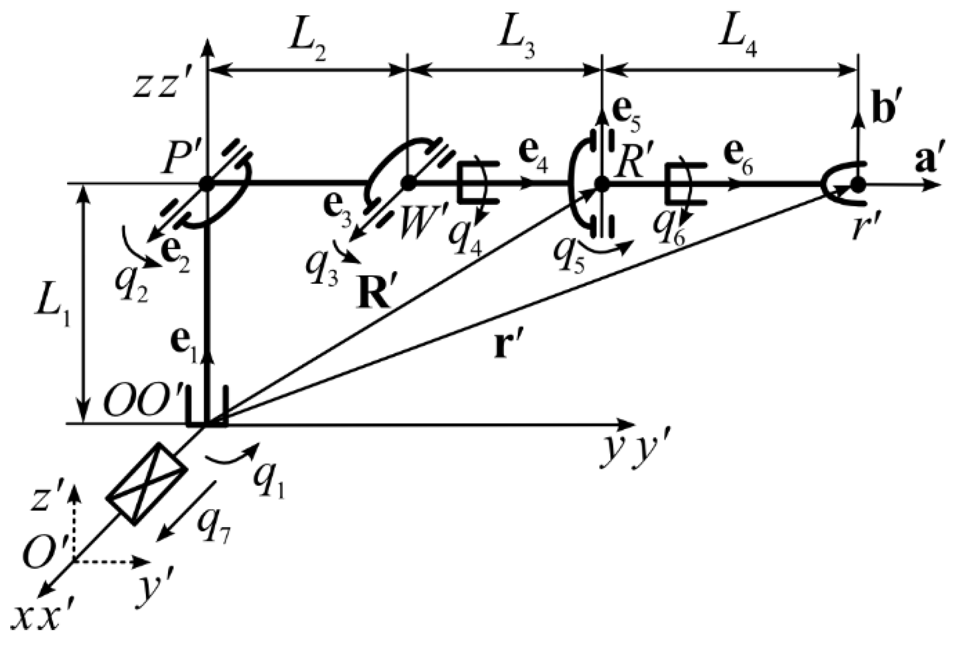
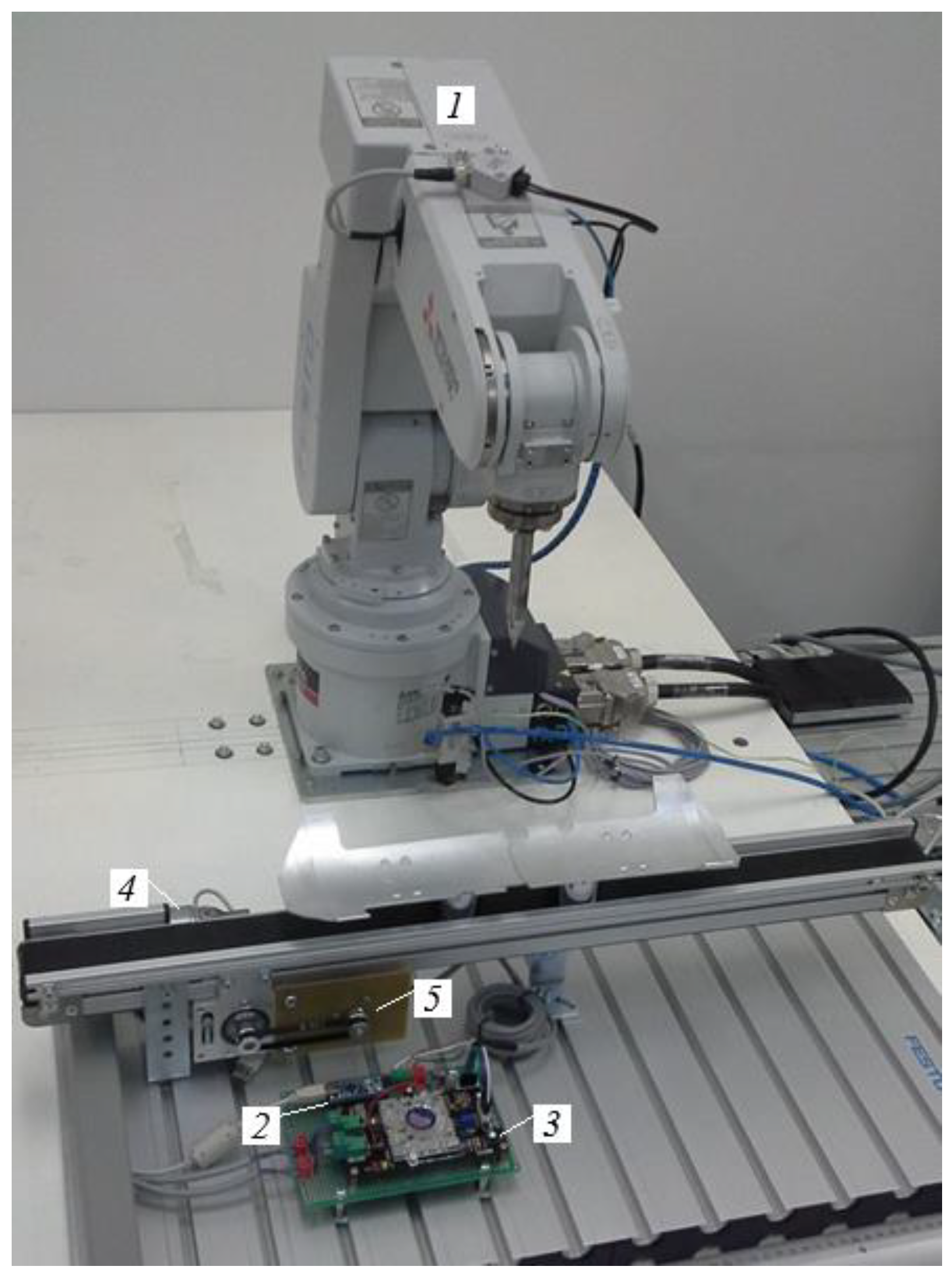
The specified task is solved for the SM using the PUMA kinematic scheme, which is installed on a movable horizontal base (see
Figure 1). In this figure, the following notation is used:
Oxyz is the absolute coordinate system (CS);
O′
x′
y′
z′ is the CS associated with the movable SM base, located at point
O′;
qi is the generalized coordinate of the
i-th DoF of the SM
;
ei is the unit vector coinciding with the joint axes of the
i-th DoF of the SM
;
a′ = [
a′
x a′
y a′
z]
T and
b′ = [
b′
x b′
y b′
z]
T are unit vectors located in the end effector plane that determine its orientation in the CS
O′
x′
y′
z′;
R′ = [
R′
x R′
y R′
z]
T and
r′ = [
r′
x r′
y r′
z]
T are position vectors of the characteristic point of the axis of the fifth joint and the tool center point (TCP) of the SM in the CS
O′
x′
y′
z′;
R′ and
r′ are points coinciding with ends of the vectors
R′ and
r′;
W′(
W′x;
W′y;
W′z) are coordinates of the characteristic point of axis of the third joint in the CS
O′
x′
y′
z′;
Lj is the length of the
j-th link of the SM
;
L4 is distance between the points
R′ and
r′; and
q7 is the displacement value of the CS
O′
x′
y′
z′ along the axis
Ox.
The CS Oxyz and O′x′y′z′ either coincide (if q7 = 0) or their axes remain parallel. In this case, the axis Oz is always pointing vertically upward, and the axis Oy makes the right-handed CS with Ox and Oz.
The limits of generalized coordinates
qi are as follows:
where
qi min and
qi max are the minimum and maximum values of the SM coordinate
qi. The limits are equal
qi min = −π and
qi max = π
for the SM in
Figure 1.
The coordinates
qi start from the SM position shown in
Figure 1. For rotary DoF, a clockwise movement is considered negative, and a counterclockwise movement is considered positive. A rotation direction is determined relative to the corresponding vectors
ei, if an observer looks from the arrow of the vector to its base.
For the SM (see
Figure 1) it is convenient to divide the IKP solution into two parts [
5], separately for transportable
q1,
q2,
q3 and orienting
q4,
q5,
q6 DoF.
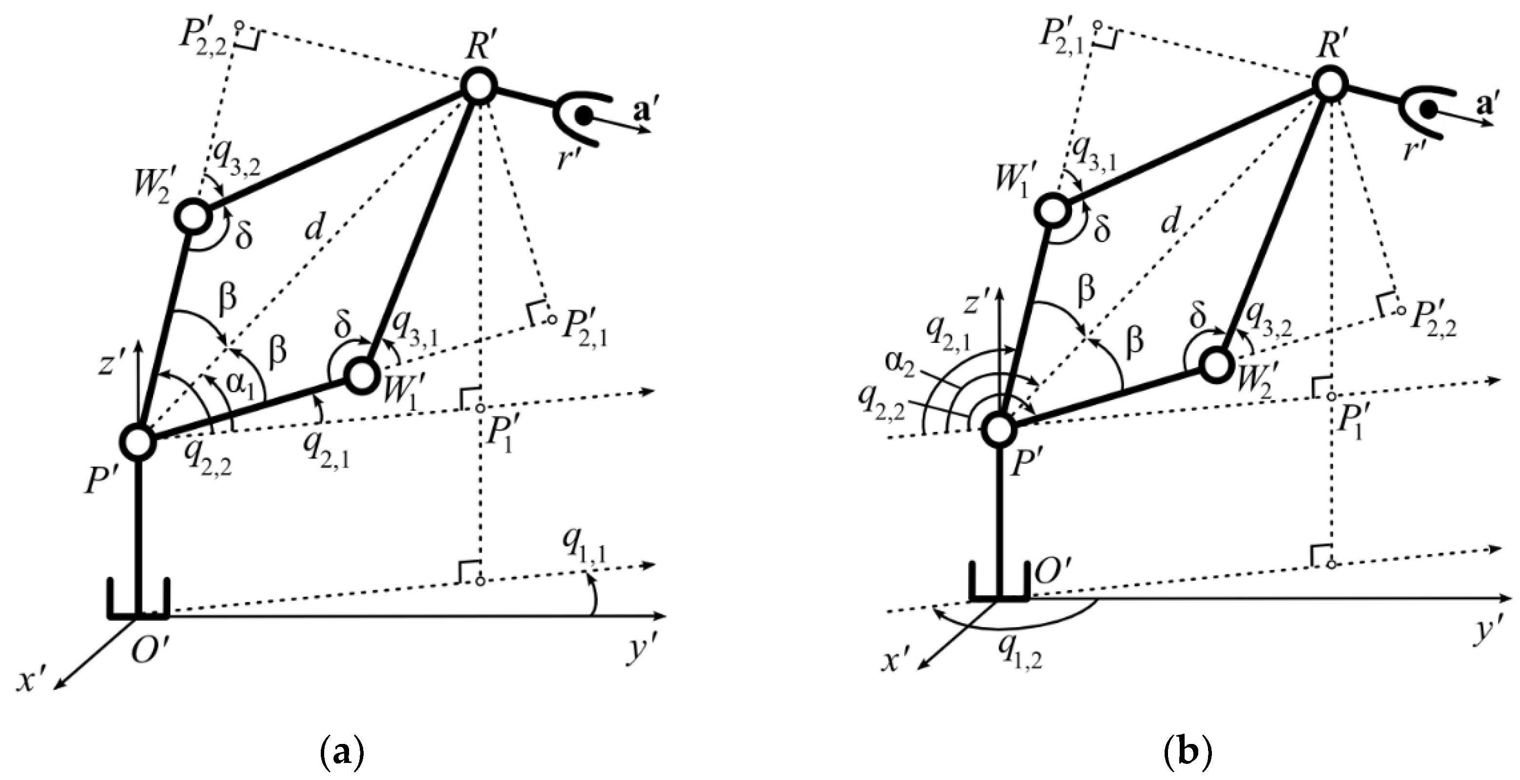
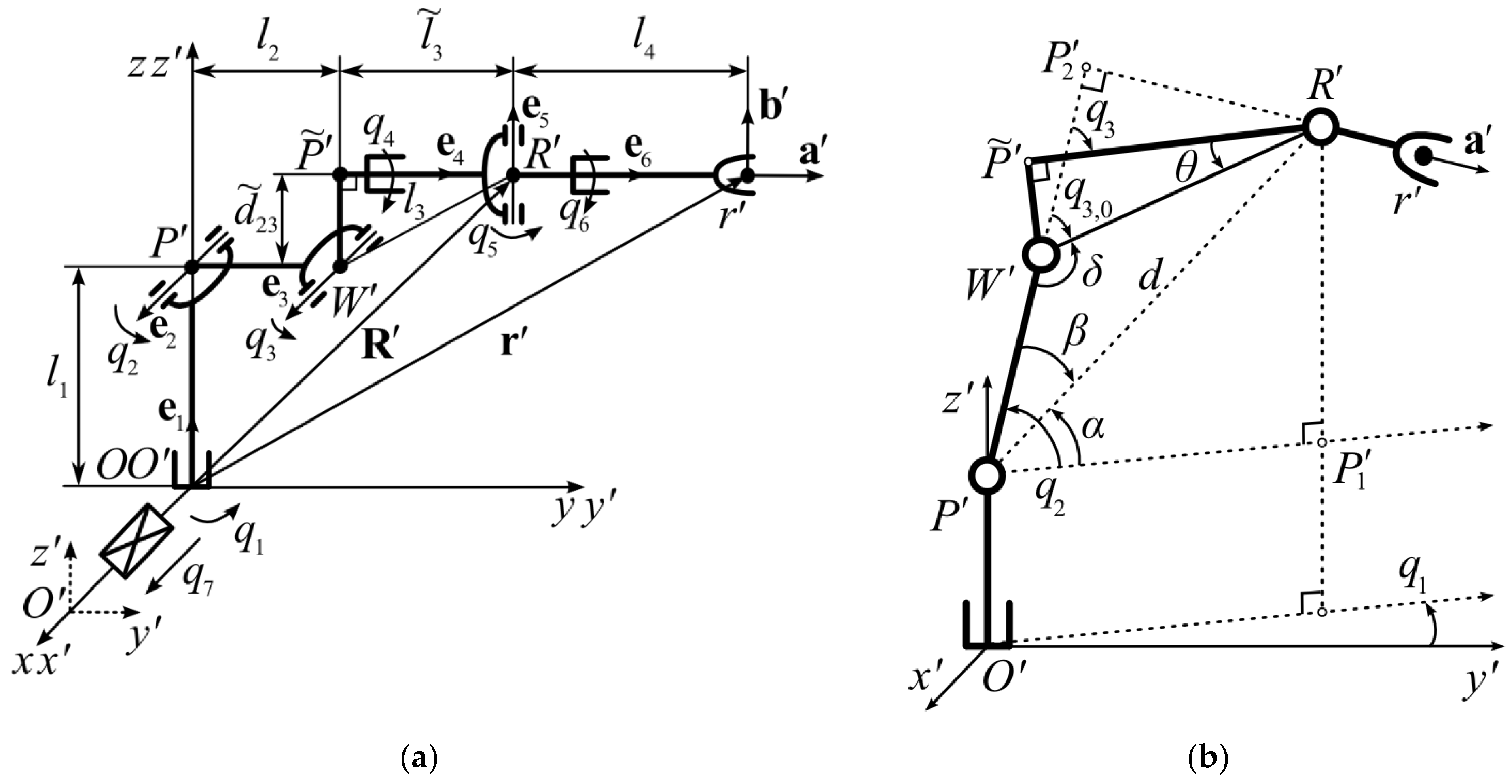
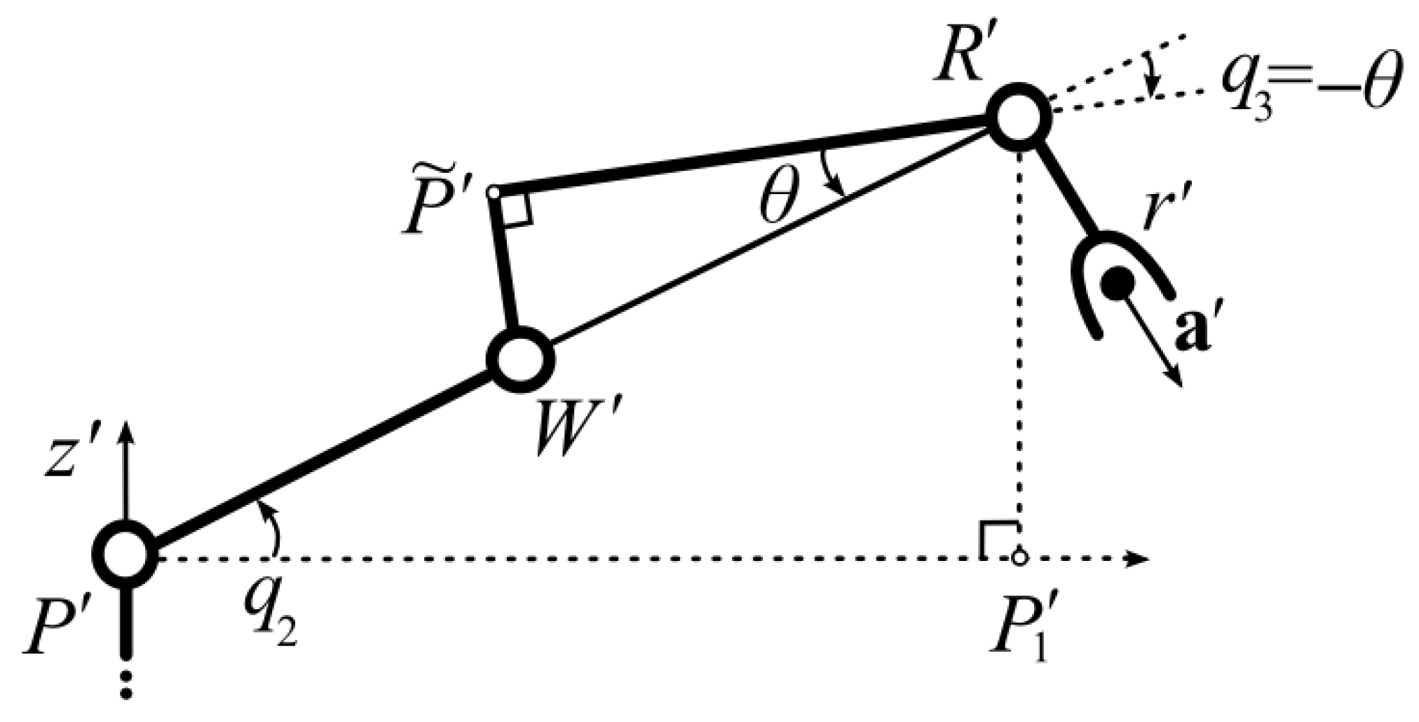
The expressions used to determine
q1–q3 can be obtained using geometry, shown in
Figure 2a,b, taking into account the coordinates of the point
R′ in the CS
O′
x′
y′
z′. The coordinates of this point are determined by the coordinates of the point
r′, the value
L4 and the spatial orientation of the vector
a′ (see
Figure 1).
Figure 2a,b show that the same location of the point
R′ in the CS
O′
x′
y′
z′ can be provided by different values of the generalized coordinates
q1 (
q1,1 or
q1,2),
q2 (
q2,1 or
q2,2) and
q3 (
q3,1 or
q3,2). This ambiguous solution of the IKP should be taken into account when forming the corresponding generalized coordinates of the SM.
Figure 2a shows that the point
R′ will have the same position in the CS
O′
x′
y′
z′ at two possible values of
q1 (
q1,1 or
q1,2), differing by the angle π; this is due to a change in
q2 and
q3. As a result, without using additional logical conditions, one can write
where
R′
x =
r′
x −
a′
xL4,
R′
y =
R′
y −
a′
yL4 [
5], and
k1 is a coefficient that determines the choice of one of two possible SM configurations (
k1 is equal to 0 or 1 if atan2(
R′
x,
R′
y) ≥ 0, otherwise −1). The choice is as follows:
q1,1 for
k1 = 0 and
q1,2 for
k1 = ±1. Moreover, the turn through the angle π should be carried out in the direction for which
q1 does not go beyond the range [−π; π]. Therefore, the sign of
q1,2 must be opposite to the sign of
q1,1 calculated above.
When determining
q2 and
q3, all possible SM configurations are considered, taking into account the different position of the characteristic point
W′ of the axis of the third joint (see points
W′
1 and
W′
2 in
Figure 2a,b, which correspond to different pairs of angles
q2,1,
q3,1 and
q2,2,
q3,2).
The value
q3 can be defined as follows:
where
si = sin
qi,
ci = cos
qi.
To determine
c3, it is possible to use any of the equal triangles (all their sides are equal)
P′
W′
1R′ or
P′
W′
2R′ (for
q1 =
q1,1 in
Figure 2a), where
P′(0; 0;
L1) are coordinates of the characteristic point of axis of the second joint in the CS
O′
x′
y′
z′. Using the cosine theorem for these triangles, when
(cos
δ = cos(π −
q3,1) = cos(π +
q3,2) = −
c3), where
δ is angle between the second and third SM links adjacent to the opposite angles
q3,1 and
q3,2 (
q3,1 = −
q3,2) for its different (see
Figure 2a) configurations, and the side length
P′R′ is equal to
, and
R′
z =
r′
z −
a′
zL4 [
5],
c3 can be written as follows:
The expression used to determine
s3 is as follows:
where
k2 = ±1 is a parameter that determines the sign of
s3 for the corresponding (of two) SM configurations (see
Figure 2a). By substituting (4) and (5) into (3), it is possible to uniquely determine the possible values
q3,1 (for
k2 = −1) and
q3,2 (for
k2 = 1).
The possible values of the
q2 (see
q2,1 and
q2,2 in
Figure 2a,b) can be determined as follows:
where
α is the angle between the horizontal plane passing through the point
P′ and the straight line
P′R′, which is equal to
α1 for
k1 = 0 or
α2 for
k1 = ±1;
β is the angle between the second link and the straight line
P′R′ (its sign coincides with sign of
q3); and
P′
1(
R′
x;
R′
y;
L1) are the projection coordinates of the point
R′ on the horizontal plane passing through the point
P′, in the CS
O′
x′
y′
z′.
From the triangle
P′
P′
1R′, for
q1 =
q1,1 (see
Figure 2a), tg
α1 =
P′
1R′/
P′
P′
1 = (
R′
z −
L1)/
. From this expression,
α1 can be written as follows:
and for
q1 =
q1,2 (see
Figure 2b), the angle
α is equal to
The angle
β can be determined from the equal triangles
P′
P′
2,1R′ or
P′
P′
2,2R′ (see
Figure 2a), where
P′
2,1 and
P′
2,2 are intersection points of perpendiculars omitted from point
R′ to lines
P′
W′
1 and
P′
W′
2. For the triangle
P′
P′
2,1R′, the equality of tg
β =
P′
2,1R′/(
P′
W′
1 +
W′
1P′
2,1) = (
L3sin
q3,1)/(
L2 +
L3cos
q3,1) is true. Since
q3,1 = −
q3,2, then the angle
β is equal to
Considering the values and signs of α1 (or α2) (7)–(8) and β (9), the generalized coordinate q2 (6) can be uniquely determined.
To calculate the other generalized coordinates
q4–
q6, taking into account the extended range of their changes, the expressions previously obtained in [
5] are used as initial ones:
where
s23 = sin(
q2 +
q3) and
c23 = cos(
q2 +
q3).
The expressions (10)–(12) are valid for the unambiguous solution of the IKP for the considered SM, only when q4–q6 change in the ranges [0; π]. Therefore, it is necessary to modify these expressions to consider the ranges [−π; π].
When determining the coordinate
q5 (11), which depends only on
q1–
q3, it is necessary to take into account two different SM configurations, at which
q5 takes values with opposite signs and the required orientation of the vector
a′ (see
Figure 1) is provided by different angles
q4. In view of the above, (11) should be rewritten as
where
k3 is parameter equal to ±1 and determines the current configuration of the SM associated with different signs of
q5.
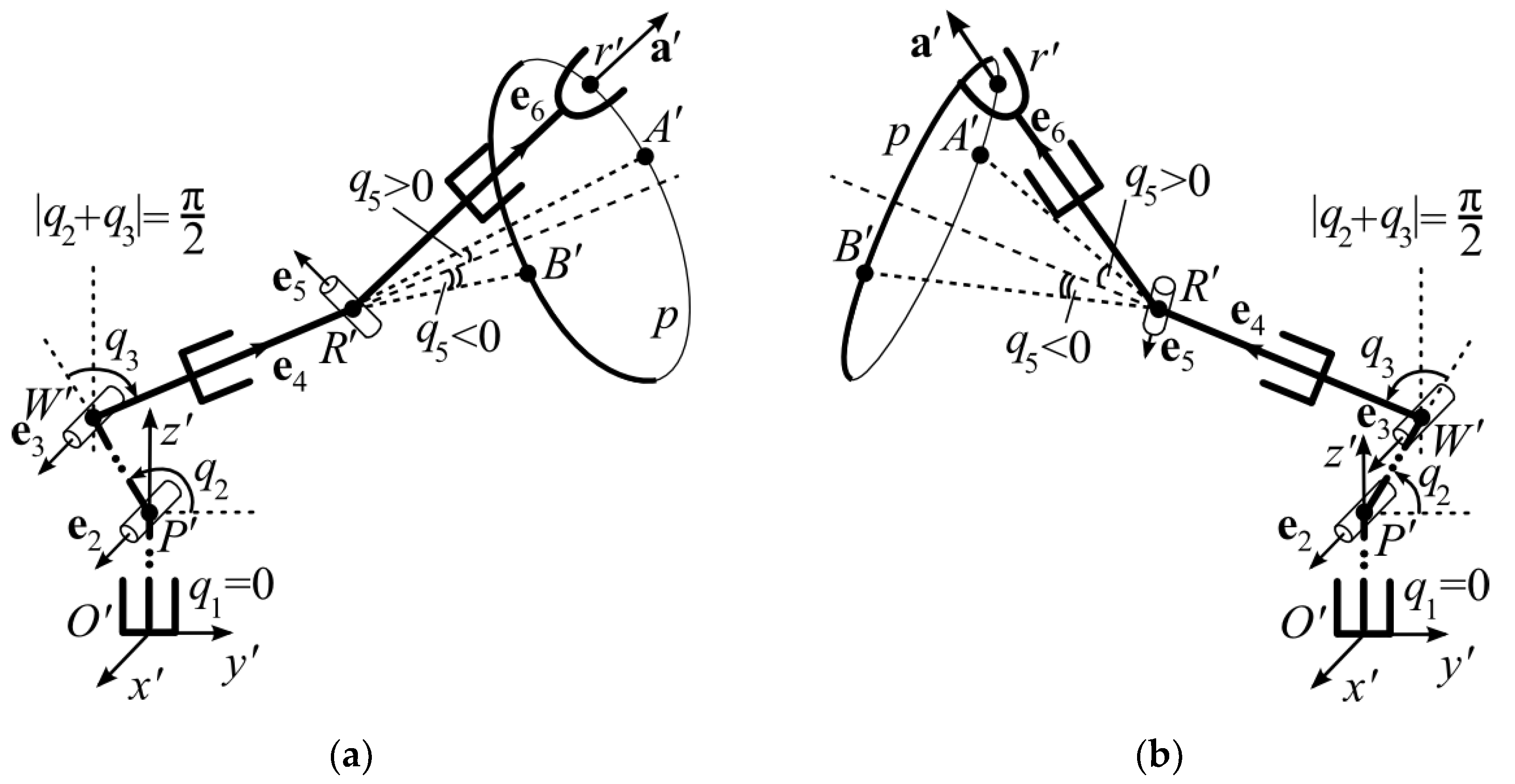
Taking into account (10), only the modulus of q4 can be determined. Therefore, to determine the sign of q4, one should obtain the logical conditions that take into account the permanent coincidence of the vectors e6 and a′. To obtain these conditions, it is necessary to take into account that when q4 changes the directions of rotation, and q1–q3 (2)–(9) and q5 (13) are fixed, a different projection behavior (decrease or increase) of e6 onto the O′z′ axis is observed.
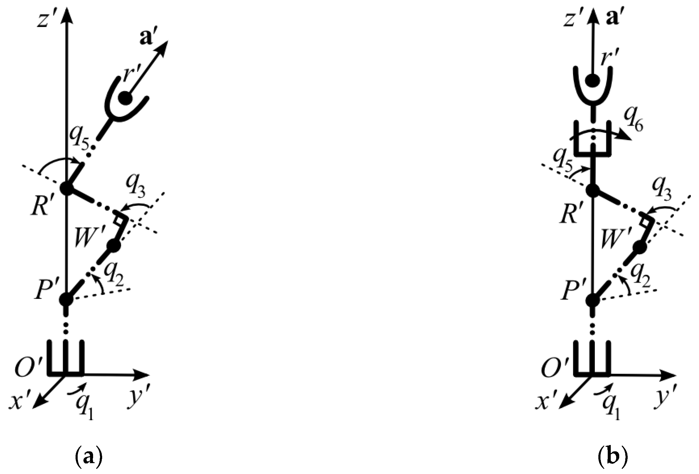
In
Figure 3a,b, two variants of the position of the SM joints are shown. An analysis of these configurations makes it possible to determine the sign of
q4. To simplify the explanations, it is assumed in these figures that
q1 = 0. Therefore, the first three SM links are located in the
O′
y′
z′ plane, and the angles
q2 and
q3 are different, but such that both figures are symmetric about the
O′
x′
z′ plane. In these figures, the vectors
e4 and
e6 do not coincide, since the angles
q5 ≠ 0. Therefore, when
q4 changes and
q5 = const, the point
R′ moves along the circle
p.
If the vector
e5 lies in the plane
O′
y′
z′, then it is assumed that
q4 = 0, and then the vector
e6 is located in the plane in which the vector
e4 also lies, which is perpendicular to the vector
e5. In this case, depending on the sign of
q5 ≠ 0, vectors
e6 in both figures will take positions
R′A′ or
R′B′, and their projections on the axis
O′
z′ will be equal to
s23c5. In this case, the positions
R′A′ will correspond to
q5 > 0, and the positions
R′B′—
q5 < 0. The position of the last SM link (see
Figure 3a) can correspond to two different pairs of angles
q4 and
q5 (in typical ranges [−π; π]), for example, π/4 and π/6, and -3π/4 and −π/6, respectively. In addition, in
Figure 3b, there are two different pairs of these angles: −π/4 and π/6, and 3π/4 and −π/6.
Figure 3a,b show that for vectors
a′ and
e6, the condition
a′
z >
s23c5 is true.
Figure 3a shows that if |
q2 +
q3| < π/2 and
q5 > 0, then when the TCP moves from position
R′
A′ to position
R′ along the circle
p q4 > 0, and if
q5 < 0, then
q4 < 0. If |
q2 +
q3| > π/2 and
q5 > 0 (see
Figure 3b), then
q4 < 0, and if
q5 < 0, then
q4 > 0.
It is easy to show that if
a′
z <
s23c5 (these SM configurations are not shown in
Figure 3a,b), then in the above situations, the sign of
q4 should be reversed. As a result, taking into account (10), in general form, the angle
q4 can be written as follows:
where sign(
x) = 1, if
x ≥ 0, otherwise −1;
k4 =
a′
z −
s23c5,
k5 = π/2 − |
q2 +
q3|.
To satisfy the condition q5 ≠ 0 in (14), the synthesized SM control system prevents the complete zeroing of q5. The sign of q6 (12) is determined by the mutual position of vectors γ = [γx γy γz]T = e5 × b′ and a′. If these vectors coincide, then the angle q6 ≥ 0, else q6 < 0. If the vectors γ and a′ coincide, their scalar product satisfies the inequality k6 = γxa′x + γya′y + γza′z ≥ 0, otherwise it is negative, where γx = b′z(s1s4 − c1s23c4) − b′y(c23c4), γy = −b′z(c1s4 + s1s23c4) + b′x(c23c4), and γz = b′y(c1s4 + s1s23c4) − b′x(s1s4 − c1s23c4).
As a result, taking into account the sign, (12) can be rewritten as follows:
After obtaining the expressions that can be used to calculate all generalized coordinates q1–q6 (see (2)–(9) and (13)–(15)), taking into account all possible SM configurations, one of them must be chosen; for this, when the SM passes from its initial position to the final, the SM DoF is as far as possible from its limits and the SM, namely from its singular positions (their details will be discussed below). This configuration is uniquely specified by the vector K = [k1 k2 k3]T.
4. Description of Indicators Detecting the Approach of the Manipulator to Its Constraints and Singular Positions
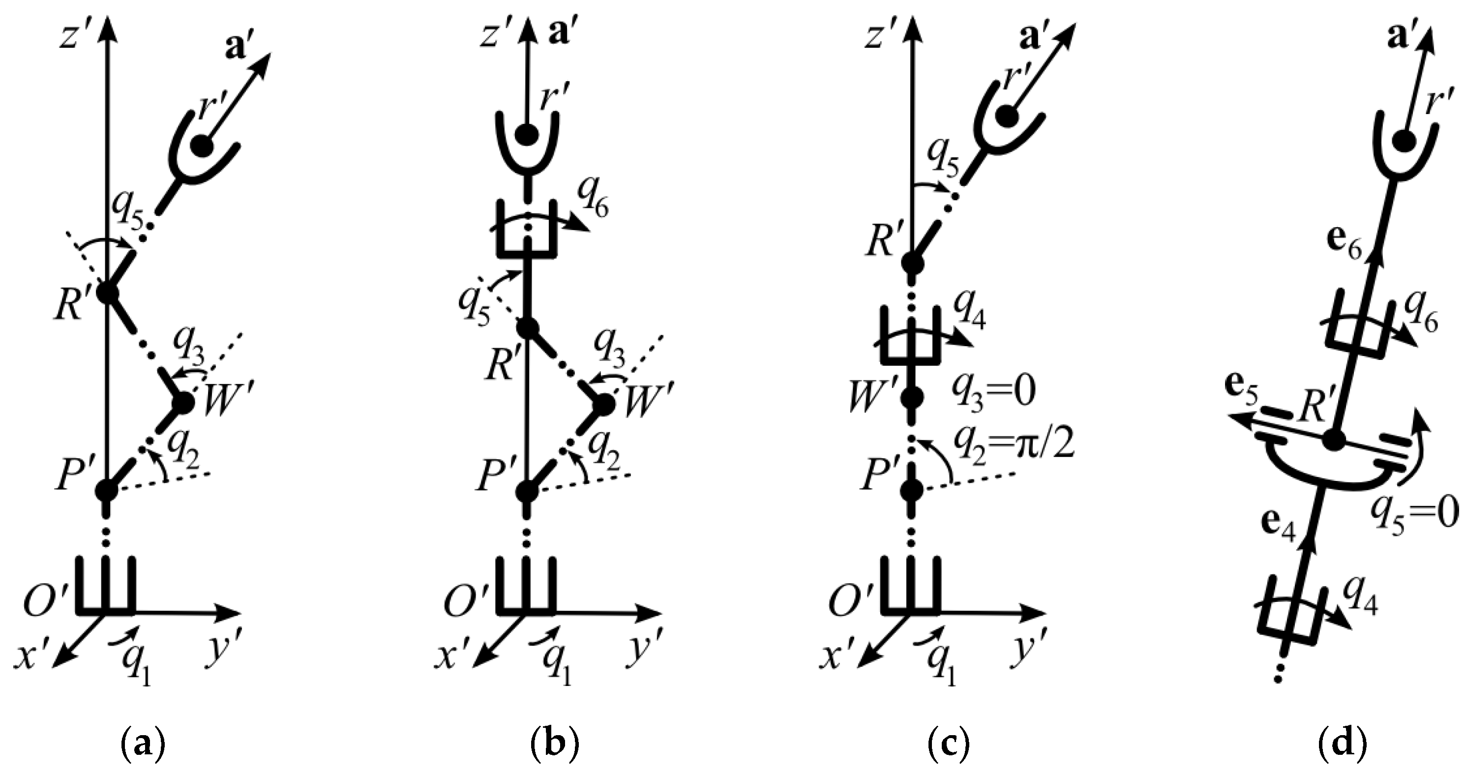
As noted earlier, when solving the IKP of the indicated SM, it is necessary to consider its four singular positions (see
Figure 4). In these positions, an ambiguous IKP solution arises and, therefore, unpredictable reversals appear in advance in some DoF.
At present, to avoid singular positions, universal numerical methods are widely used to solve the IKP. They involve performing iterative calculations, often (but not necessarily) associated with the calculation of pseudo-inverse Jacobi matrices [
13,
16,
27]. Some papers, including [
28,
29], are devoted to the numerical solution of the IKP without computing the pseudoinverse Jacobi matrices. In these papers, a heuristic method is presented that is characterized by a high rate of convergence, which makes it possible to perform IKP solutions in just a few iterations, but the presence of redundant DoF significantly increases its computational complexity. Therefore, singular positions for the considered SM will be described below, and then a way to avoid them without the use of powerful computing devices will be proposed.
In the first singular position (see
Figure 4a), the projection of
R′ onto the horizontal plane
O′
x′
y′ coincides with the origin of coordinates
O′. In this position, many different values of the angle
q1 are possible, which will correspond to different
q4–
q6. In the second singular position (see
Figure 4b), the origin of coordinates
O′, as well as points
R′ and the TCP
r′, lie on the same vertical line, and it is possible that there are many pairs
q1 and
q6. In the third singular position (see
Figure 4c), the origin of coordinates
O′, points
W′ and
R′ lie on the same vertical line, and the coordinates
q1 and
q4 are not uniquely determined. In the fourth singular position (see
Figure 4d), the last links of the SM lie on one straight line,
q5 = 0 and the coordinates
q4 and
q6 are undefined.
The appearance of the described singular positions and SM entrances to the constraints can be prevented by using an additional (redundant) linear DoF
q7 (see
Figure 1). A system for forming the reference signal for controlling this redundant DoF is presented in [
5]. For its implementation, several special indicator functions are introduced. Their current values should indicate the approach of the SM to its special (critical) positions.
The value of the first indicator
J1 tends to be 1 when any of the generalized coordinates
qi approach their limits ±π, and it equals 0 when all DoF are in their average positions. As a result, the following expression can be used as the first indicator:
The value of the second indicator
J2 tends to be 1 when the SM approaches the first three singular positions, at which point
R′ is located on the
O′
z′ axis associated with the base of the SM. The expression for calculating this is as follows:
The third indicator
J3 indicates the approach of the SM to its fourth singular position, at which
q5 = 0. Its value can be calculated as follows:
The value of the fourth indicator
J4 is equal to 1 if the WT approaches the border of the working area, where
q3 = 0. Its value can be calculated as follows:
During the operation of the system, changes in these indicators (16)–(19) are monitored. If any of them show that the SM is approaching an undesirable position, then this system ensures the elimination of the above SM positions due to the redundant movement of the base along the q7 coordinate.
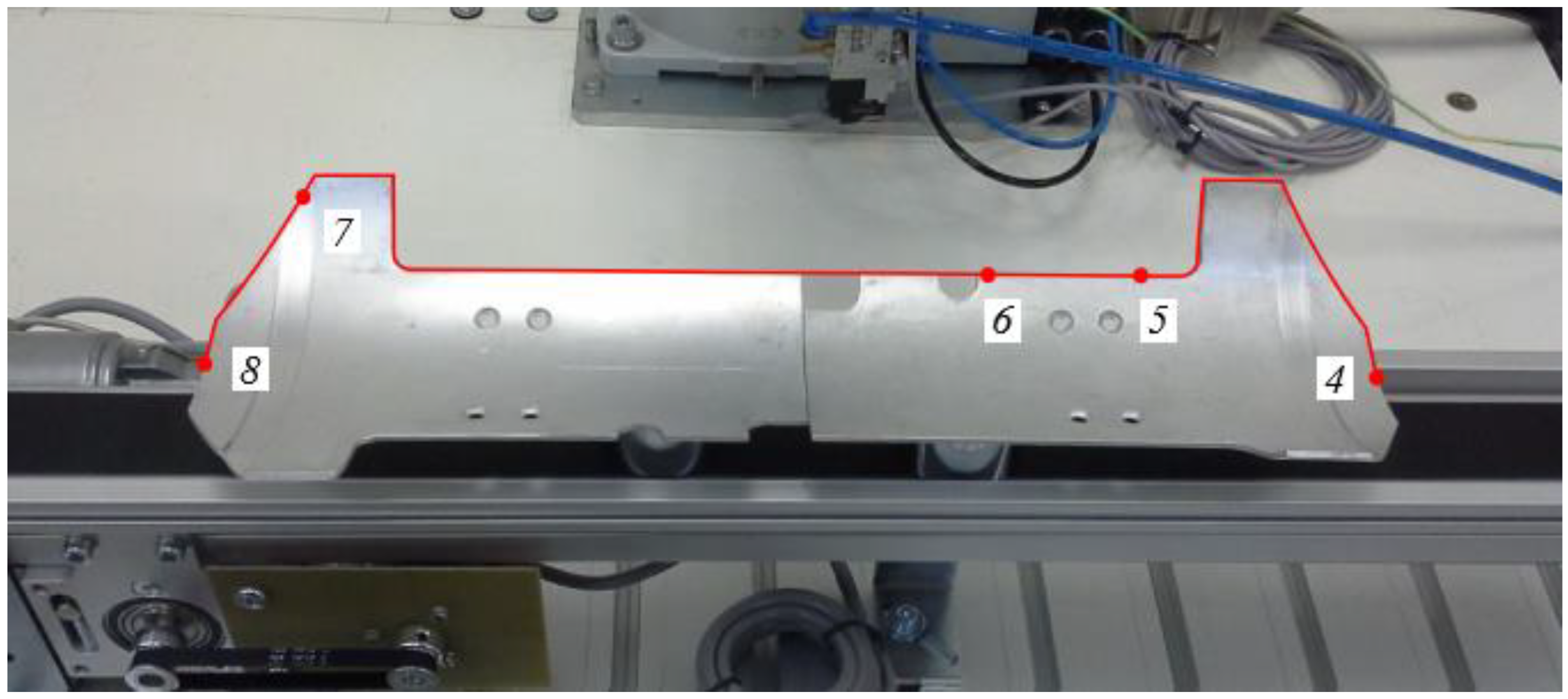
5. Results of Simulation
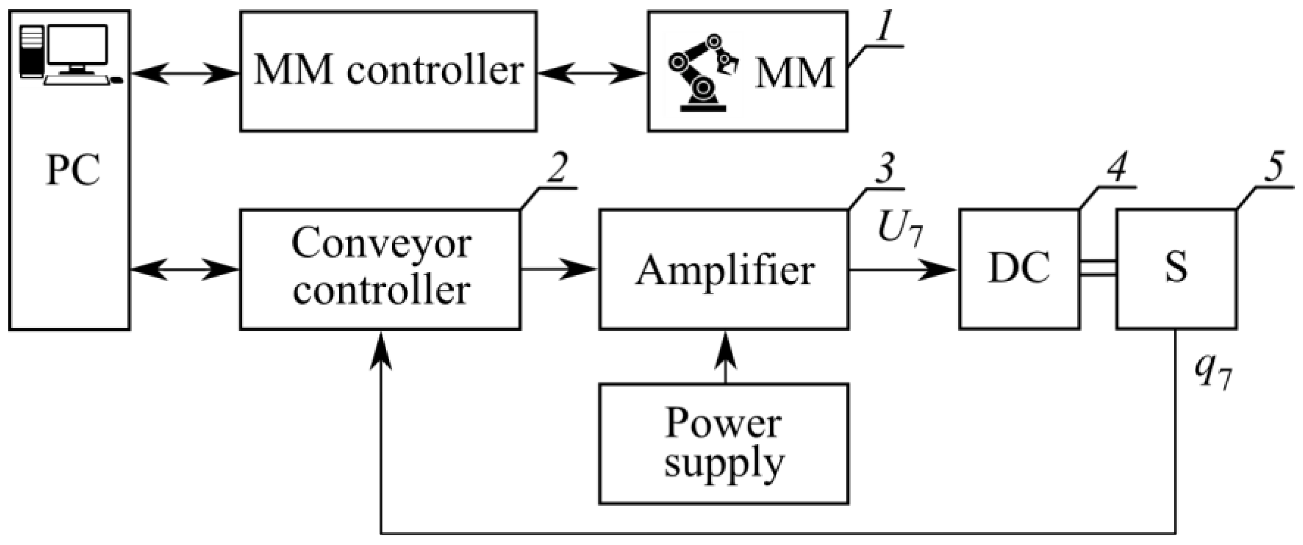
The simulation study of the developed system for generating reference signals was carried out in MATLAB Simulink for the SM (see
Figure 5); this is part of the production chain, such as those described in [
30,
31]. A new detail appears in the working area of this robot at fixed (discrete) times. The equations of the SM motion were solved by means of fourth-order Runge–Kutta methods (ode45).
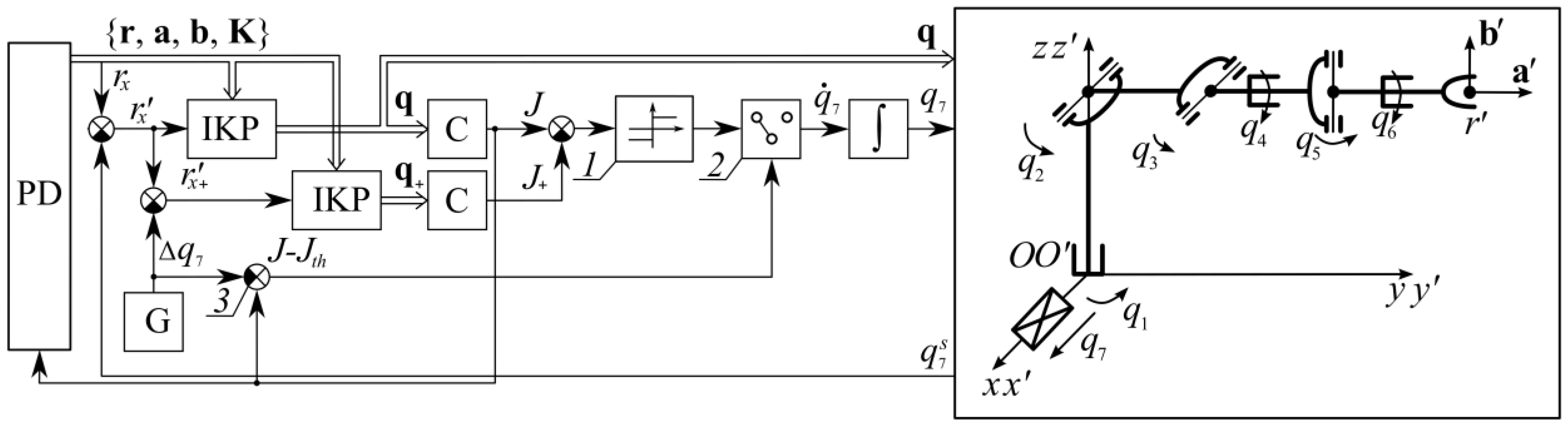
Figure 5 shows a generalized simulation scheme that provides the generation of all main reference signals
q1–
q7. In this figure, the following notations are used: PD is a program device generating the current reference values of the TCP coordinates;
is the position of redundant DoF measured by a sensor; G is a generator of a constant signal Δ
q7 > 0; IKP are blocks for solving the SM IKP, which form vectors of generalized coordinates
q = [
q1 q2 …
q6]
T and
q+, respectively, for two different positions of the SM base,
q7 and
q7 + Δ
q7; C are controllers that calculate the current values of all four indicators (16)–(19) and select the largest
J and
J+ from them, respectively, for two different positions of the SM base,
q7 and
q7 + Δ
q7;
1 is a relay element that determines the magnitude and sign of constant speed
;
2 is a relay providing a connection from the output of the relay element 1 to the input of the electric drive controlling the coordinate
q7; and 3 is an adder that generates the
J-
Jth signal (its input from the block G has a gain
Jth/Δ
q7).
The presented system works as follows.
In PD, taking into account the information from the vision system, a reference trajectory of the WT movement is generated. At the same time, at the output of this block, the reference values of the elements of vectors r, a and b in CS Oxyz are formed, as well as the vector K, which uniquely determines the current configuration of the SM. Taking into account these vectors and the continuously measured displacement of the SM along the redendant coordinate q7, the elements of the vector q are calculated in the IKP block, which are processed by the SM actuators, ensuring the movement of the WT along the trajectory.
When the SM approaches the specified undesirable positions, the redundant DoF
q7 is activated. To control it in this system, the IKP (see second block IKP in
Figure 5) is additionally solved for the SM position, shifted along the
Ox axis at a distance of
+ Δ
q7. Then, for both positions (
and
+ Δ
q7) in the blocks C, the values
J and
J+ of the largest of the indicators (16)–(19) are calculated. Then, at the output of relay block 1, the direction in which the SM base must be shifted is determined in order to reduce the
J and therefore avoid unwanted positions. In block 2, there is a switch that connects (or disconnects) the
q7 actuator, taking into account the sign of the difference
J −
Jth.
The generalized coordinates of the SM vary in the ranges [−π; π] (1). The lengths of the SM links are
L1 =
L2 =
L3 = 0.5 m and
L4 = 0.15 m, their masses are
m1 = 25 kg and
m2 =
m3 = 15 kg, and their cargo weight is
mg = 5 kg. The inertia moments
Jsi and
Jni of the
i-th SM links that are relative to their longitudinal axes and axes passing through the mass centers, and are perpendicular to their longitudinal axes, are
Js1 = 0.1 kgm
2,
Js2 = 0.007 kgm
2,
Js3 = 0.005 kgm
2,
Jn2 = 0.55 kgm
2 and
Jn3 = 0.31 kgm
2. DC motors of independent excitation or permanent magnets are used as the SM actuators. They have a well-known and verified mathematical model (see, for example [
32]) that uses the following parameters:
Kyi = 1,
ipi = 100
;
Ri = 0.5 Ohm,
Li = 0.01 H,
KMi = 0.04 Nm/A,
Kωi = 0.04 Vs/rad,
JEi = 10
−3 kgm
2 (
and 7); and
Ri = 1.4 Ohm,
Li = 0.02 H,
KMi = 0.06 Nm/A,
Kωi = 0.06 Vs/rad,
JEi = 0.3∙10
−3 kgm
2 . The nominal inertia moment
Jnom i = 10
−4 kgm
2 of the shaft of the
i-th (
and 7) actuator and the rotating parts of the gearbox is used in the self-tuning regulators [
32] to compensate for the force–moment interactions between the SM DoF. Typical PID controllers are used in closed-loop actuators. The movement speed of the WT along a reference trajectory is set equal to 0.5 m/s, but in practice it can be variable and be adjusted according to the [
33].
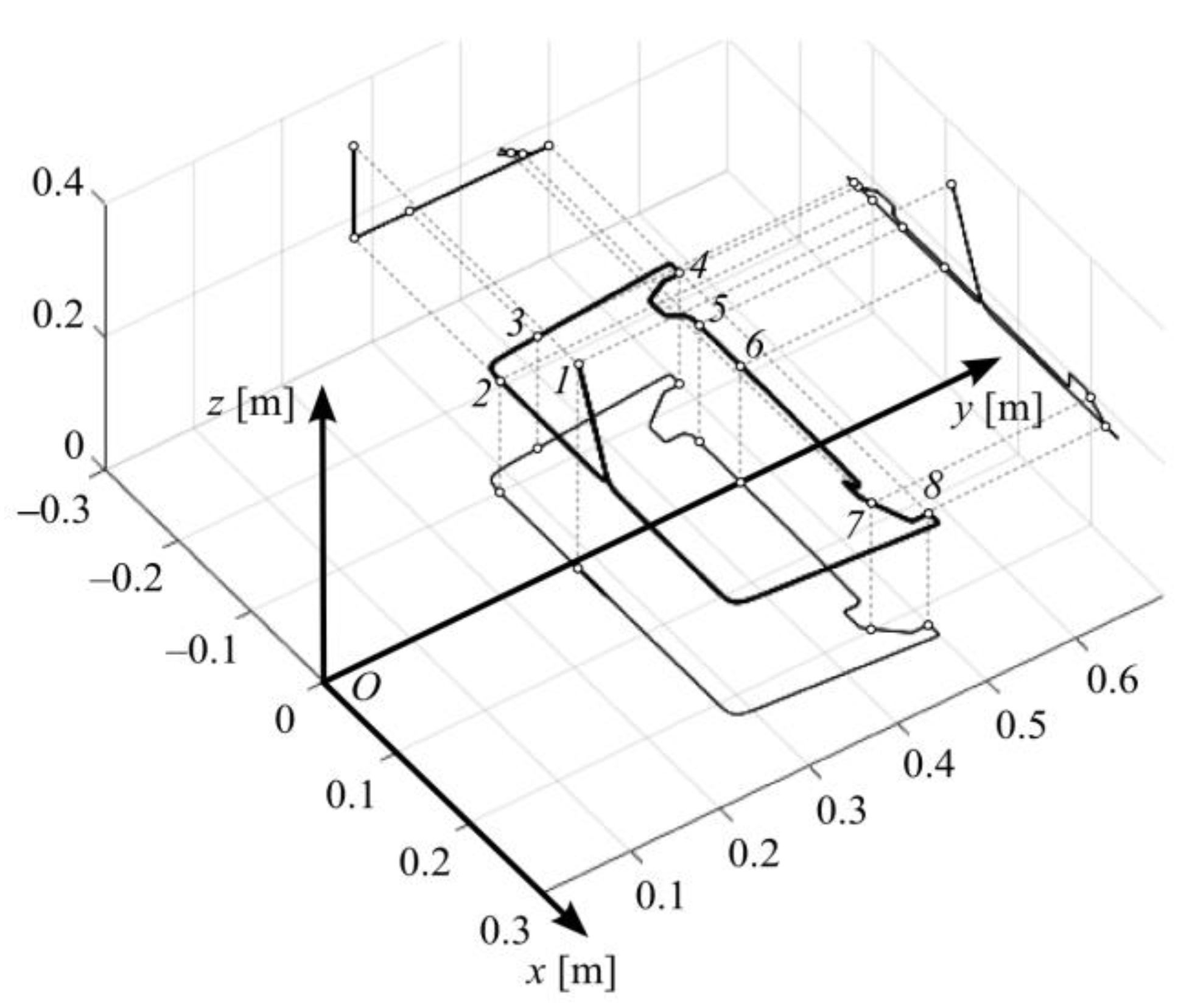
Figure 6,
Figure 7 and
Figure 8 show the MATLAB simulation results of the operation of the 6-DoF SM installed on the movable base (see
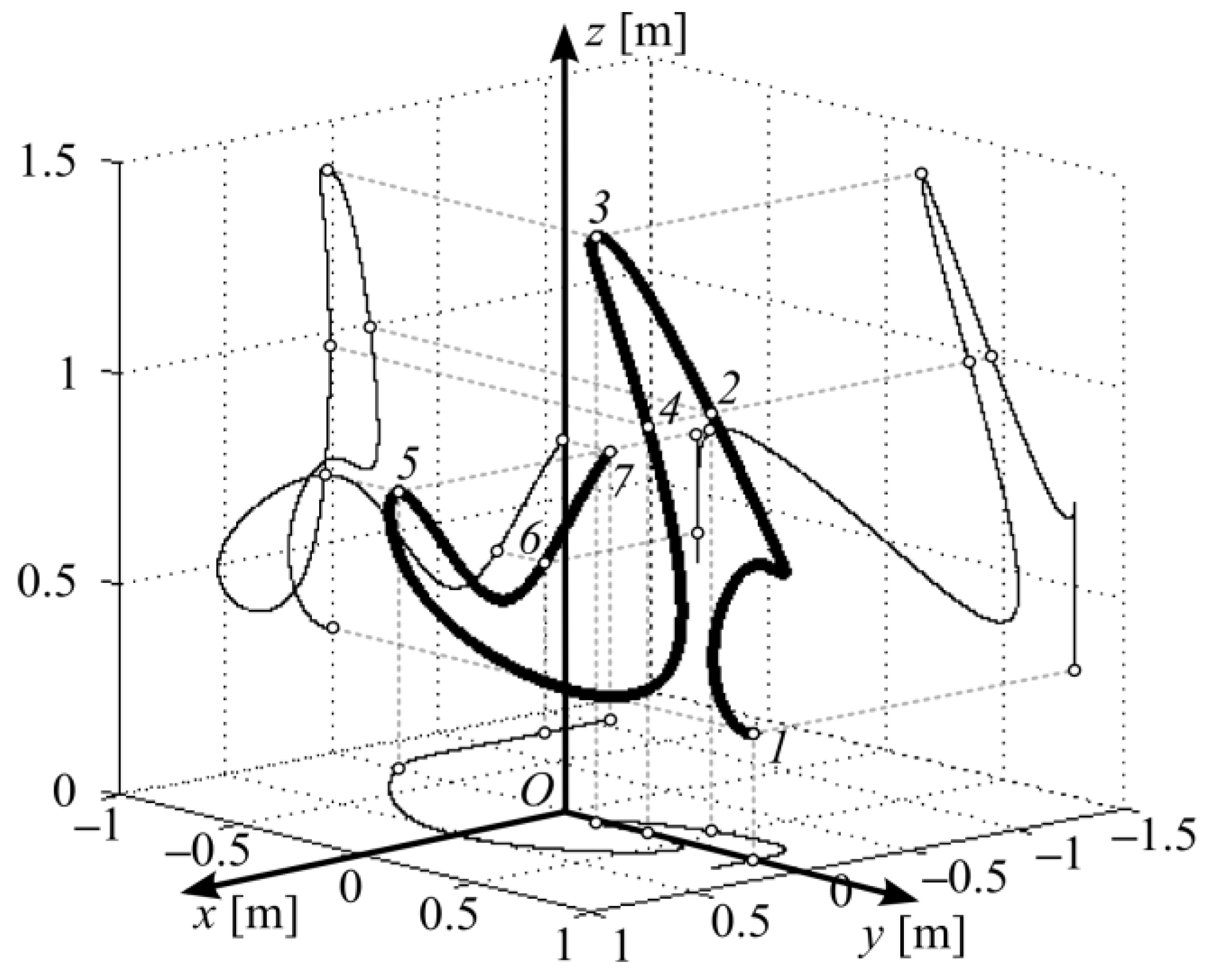
Figure 5). The SM TCP moved along a complex spatial trajectory (see
Figure 6), formed by using parametric splines of the third order [
34]. This trajectory began at starting point 1 and then successively passed points 2–7. For this developed system, the elements of the matrix
K were automatically defined as
K = [0–11]
T. The trajectory shape and WT orientation were chosen such that at
q7 = 0, when the CS
Oxyz and
O′
x′
y′
z′ coincided, the SM successively entered the undesirable positions described above.
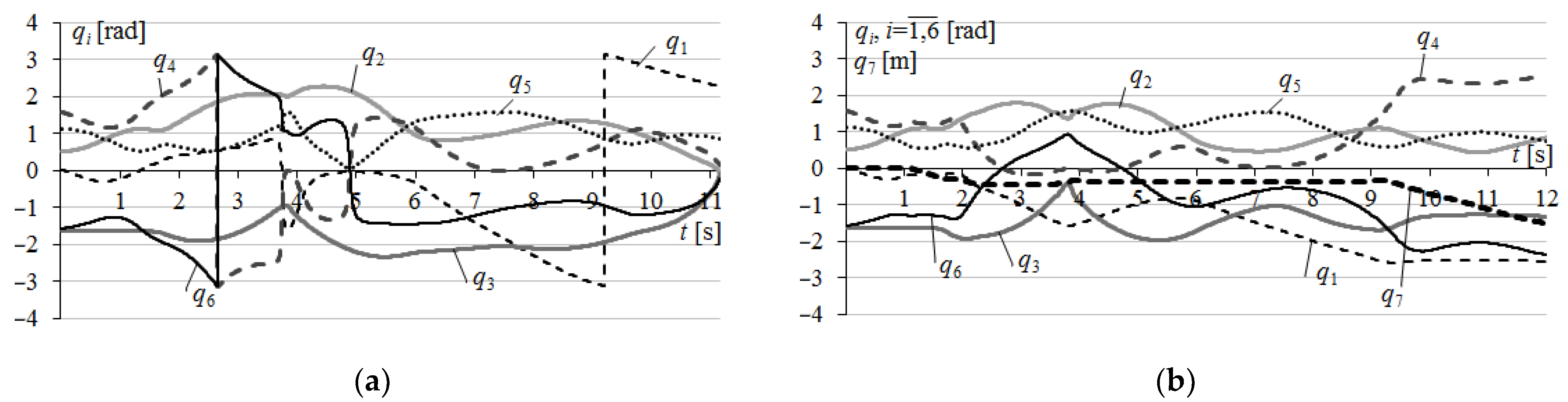
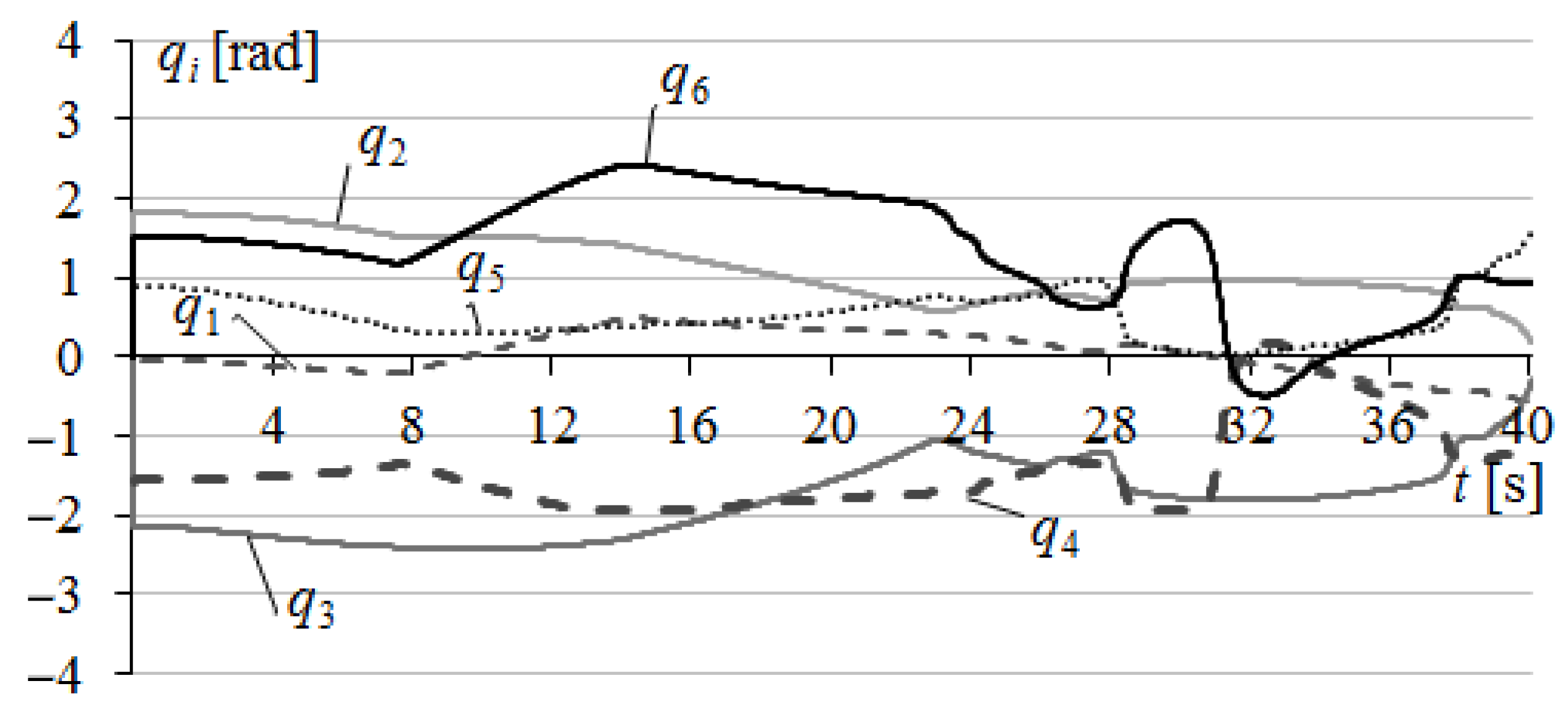
The behavior of the reference values of the generalized coordinates
q1–
q6 when the WT moves along the reference trajectory is shown in
Figure 7a. During this movement, the SM enters two different singular positions; the three DoF reached their limits three times, and once at the end of movement the WT reached the border of the SM working area.
When the TCP passed point 2, the sign of
k4 in (14) was changed. This led to the reference values of the generalized coordinates
q4 and
q6, which were reached in the limits (see the time moment 2.6 s in
Figure 7a), sharply changing their values. When passing point 3, the SM approached the first singular position (see
Figure 4a), at which point
R′ was located strictly vertically above point
O′ and the values
q1,
q4,
q6 changed sharply (see 3.7 s in
Figure 7a). When passing point 4, the SM entered the fourth singular position (see
Figure 4d), at which
q5 = 0 (see 4.9 s in
Figure 7a) and reverses occurred in its fourth and sixth DoF. When passing point 5, the first DoF reached its limit (see 9.2 s in
Figure 7a), and then sharply changed its value from −π to π. At point 6, the WT reached the border of the working area when
q3 = 0 (see 11.2 s in
Figure 7a), and the SM emergency stopped without reaching the required point 7.
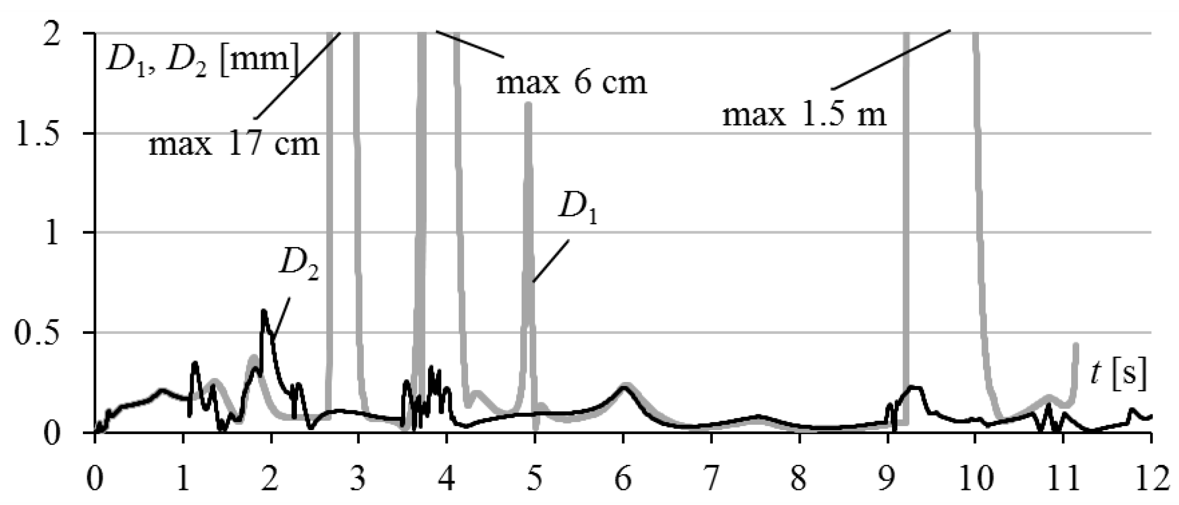
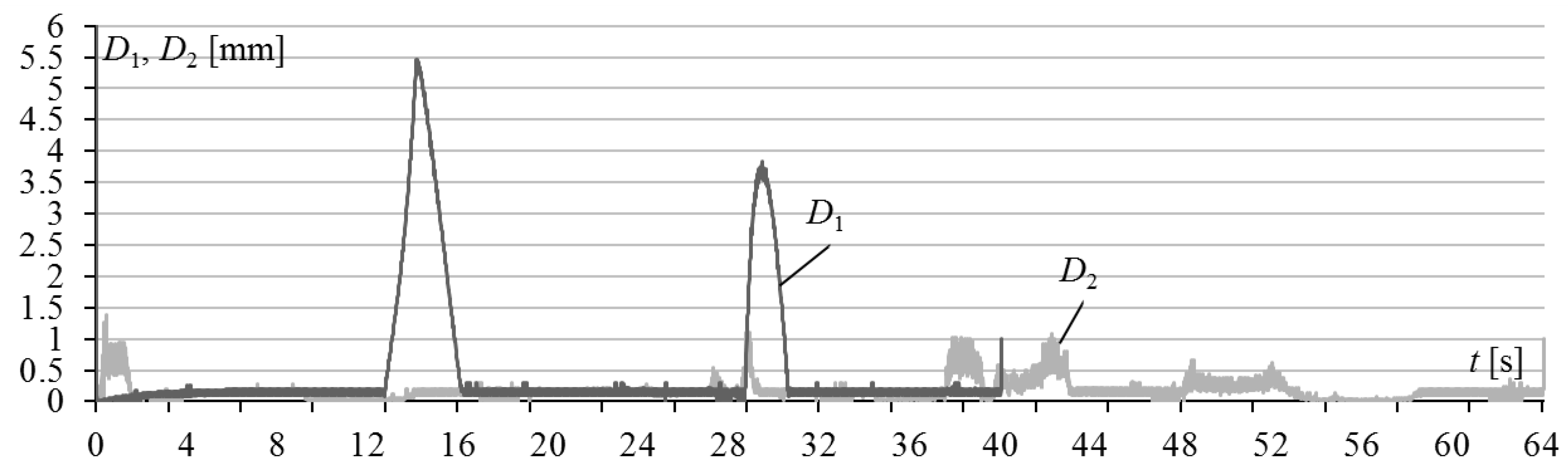
Obviously, the emerging step changes in the reference values
q1–
q6 (see
Figure 7a) could not be processed instantly by the SM actuator. As a result, the deviation
D1 of the TCP from the reference trajectory near the special sections increased to unacceptable values—from min 1.7 mm to max 1.5 m (see
Figure 8).
To prevent these negative situations, the proposed system was used, which ensures the movement of the SM base along the coordinate
q7 while its configuration approaches the problem areas. The reference values
q1–
q6 generated by the system, taking into account the real value
q7, which also changes in time during the process of moving along the trajectory, are shown in
Figure 7b. This figure shows that the abrupt changes in the reference values in all the generalized coordinates of the SM are completely prevented, and that the deviation
D2 in the SM TCP from the reference trajectory did not exceed 0.65 mm (see
Figure 8) in all its sections and that the motion of the SM was fully completed (strictly at the end of the trajectory) at point 7 (see
Figure 6).


