A Comprehensive Multibody Model of a Collaborative Robot to Support Model-Based Health Management

Abstract

Digital models of industrial and collaborative manipulators are widely used for several applications, such as power-efficient trajectory definition, human–robot cooperation safety improvement, and prognostics and health management (PHM) algorithm development. Currently, models with simplified joints present in the literature have been used to evaluate robot macroscopic behavior. However, they are not suitable for the in-depth analyses required by those activities, such as PHM, which demand a punctual description of each subcomponent. This paper aims to fill this gap by presenting a high-fidelity multibody model of a UR5 collaborative robot, containing an accurate description of its full dynamics, electric motors, and gearboxes. Harmonic reducers were described through a translational equivalent lumped parameter model, allowing each constitutive element of the reducer to have its decoupled dynamics and mating forces through non-linear penalty contact models. To conclude, both the mathematical model and the real robot on a test rig were tested with a set of different trajectories. The experimental results highlight the ability of the proposed model to accurately replicate joint angular rotation, speed and torques in a wide range of operational scenarios. This research provides the basis for the development of a model-based PHM-oriented framework to carry out detailed and advanced analyses on the effects of manipulator degradations.

1. Introduction

Recent years have seen a significant growth in the adoption of collaborative robots (cobots) in industrial environments, since their low entry-point cost and relative simplicity has popularized the adoption of increased automation levels in small and medium enterprises [1]. Since these manipulators are largely employed in assembly lines [2], inspection [3], or repair operations [4,5], their malfunctioning might jeopardize the operators’ safety and cause unexpected downtimes. To mitigate these risks, preventive actions, such as scheduled maintenance, are usually adopted. Nevertheless, since each robot is programmed to execute a specific task, its load history and degradation rate are not equal to the ones of the same machine performing a different task. Other possible solutions are represented by stand-by working stations, backup manipulators, and fault-tolerant control algorithms [6], which, however, are not always applicable.

Within this context, condition-based maintenance represents a key technology to ensure line availability and prevent economical losses. The ability to detect a fault at its early stage allows scheduling the replacement of the faulty components during periods of lower production, or before the robot can cause any damage to the operators with which the cobot shares its workspace or the production line itself. To do so, data-driven models (DDMs) are often used to extract health indicators from the machine and predict its remaining useful life using the obtained dataset to test machine learning algorithms [7]; for example, confronting simulated acceleration and measured acceleration by means of an accelerometer mounted on the tip of the robot [8,9]. While these algorithms can also be used to detect motor failures [10], according to [11], electric faults are likely to be autonomously detected by the built-in control logic of the joint. As such, prognostics and health management (PHM) studies on robotic systems are mainly focused on the detection and classification of mechanical faults on bearings [12] and gearboxes. By adding several sensors [13,14,15,16], it is possible to obtain information about, for example, speeds and accelerations. After the definition of the dataset, the analysis of these data can be performed using, for example, generative adversarial networks [13,14,15,16] to solve the problem of data imbalance and multiscale convolutional neural network to realize the fault diagnosis of the harmonic drive. Another approach is based on the use of deep learning [13,14,15,16] to extract, optimize, and classify different features. However, the main drawback of this approach is the need for large datasets of both healthy and faulty robot behavior, which are rarely available [17,18] due to an average mean time between failures of tens of thousands of hours [19]. To overcome this limitation, a database of simulated data in the presence of faults and failures can be built through a high-fidelity model of the robot arm. Such data, together with the experimental data, can be used to train DDMs for the proper detection and classification of the failure modes to which the machine is subjected. In [20,21], the authors proposed the application of a prognostic framework based on a long short-term memory neural network and the automatic recognition of the assembly task to detect mechanical faults in a robot for roller hemming employed in the automotive sector. Another example is represented by [20,21], in which physics-based simulation models, based on the digital twin concept, are used to obtain an estimate of the remaining useful life of machinery equipment.

With this aim, several studies focused on researching kinematic analyses and calibration of anthropomorphic robot manipulators, such as the UR5 collaborative robot from Universal Robots A/S, and on the creation of its digital twin to replicate the dynamic behavior, have obtained insights on internal quantities and studied the effects of specific degradations on both its position accuracy and overall performance. In Ref. [22], the authors present a kinematic model of a 6-DoF manipulator that utilizes the Denavit–Hartenberg convention to describe the relationships between the reference frames of each joint in the robot. The same approach was followed in [23] to obtain a simplified mass-concentrated model of a 3-DoF anthropomorphic manipulator: this kind of model can be used for kinematic calibration, as in [24]. In Ref. [25], a similar approach was used to perform forward and inverse kinematics to obtain the joint angular rotations from the desired Tool Center Point (TCP) pose and vice versa. To achieve this, a specific trajectory must be followed, and the inverse dynamic modeling approach allows calculating the torques required for such a trajectory. This requires considering the inertia of the links, Coriolis forces, gravity, and every exogenous force or torque applied on the robot, as shown in [26].

However, in high-fidelity models, particularly those involved in the creation of non-nominal behavior datasets for PHM purposes, a causal forward dynamic approach is preferred since it is dynamically consistent and satisfies the fundamental laws of physics at each point of the simulation.

The ability to replicate not only the actual joint positions, but also the torques necessary to perform the desired trajectory, is crucial for several studies, such as the ones aiming to minimize the power consumption of industrial manipulators [27,28] or the ones focused on using robot digital twins to evaluate the safety and ergonomics of specific applications [29,30]. The development of accurate models allows improvements in productivity and accuracy [31] as well. For these reasons, dynamic models of increasing complexity have been developed according to the specific objective and needs [32]. One of the main purposes related to the definition of dynamic models concerns the design and testing of the control algorithms. In Ref. [33], the PID controller of the robot was tuned based on the Ziegler–Nichols method, exploiting a classic dynamic model of a robot obtained by means of Lagrange equations [23]. In Ref. [34], the authors developed a simplified dynamic model by means of the Kane equation to study a robot design environment for the use of collaborative robots for rehabilitation purposes.

Good et al. [35] investigated the robot control algorithm and underlined the importance of taking into account the interactions between the robotic arm and the electromechanical drives. The model presented in [36] enhanced the mathematical representation of the robot structure, considering a simplified electric motor model. Tarn et al. [37] developed a third-order dynamic model of the robot obtained by combining the manipulator and the motor dynamics to study the effect of a nonlinear feedback control. Here, the model received as input the motor’s armature voltage and returned as output the kinematic quantities of each joint.

An effective description of robot dynamics is necessary to achieve simulation models with high accuracy. For this reason, in both forward and inverse dynamics approaches, it is vital to know the correct dynamic parameters of the robot. On this topic, several studies concentrated on the development of identification techniques for these parameters [31], minimizing the error between the signal measured on the real robot, subjected to a proper excitation trajectory [38], and those obtained from the model simulation. Kovincic et al. [26] identified the dynamic parameters using a Moore–Penrose pseudo-inverse of the regressor of a UR5, obtaining a functional set of parameters to reproduce the robot’s trajectory. However, this approach did not include any constraints on the values of the dynamic parameters, which can lead to a physically meaningless set of parameters. To solve this problem, in [39], a different method of identification of the dynamic parameters was proposed. Such an approach offers promising results, but requires the use of additional sensors such as accelerometers to measure the motion of each joint. An alternative way to identify the dynamic parameters involves the use of statistical techniques [36]. This method can provide excellent results in terms of overlapping of the model with the experimental results, but suffers from a very loose representation of the system physics. An alternative approach was developed by Raviola et al. [40], which applied a constrained genetic algorithm minimization, taking into account also the effect of mounting configuration for different temperature conditions.

Hitherto, in the literature, the majority of dynamic models of robotic manipulators were developed with the goal of describing the macroscopic behavior of the entire system without taking into account the punctual description of each subsystem of the robot and their interaction. However, if a physics-based description of faults and degradation in the system has to be inserted for PHM analyses, a high level of detail and fidelity of the model is required, and the dynamic behavior and mutual interaction of each subsystem should be taken into account.

To solve these issues, the present paper describes a high-fidelity model of a UR5, a six-degrees-of-freedom (DoF) collaborative robot from Universal Robots A/S. Hayati’s additional kinematic parameters were introduced to model assembly errors and obtain more physically representative kinematic calibration parameters. From a dynamic perspective, the dynamic parameters were identified for the UR5 under study according to [40]. Additionally, a detailed joint model was developed to accurately model the elements of each joint, including the electric motor and the reducer. For the latter, a strain wave gear dynamic model was considered together with the description of the internal interactions between its main elements, enabling a comparison between real robot currents and those generated by the model. The proper modeling and implementation of the reducer in the description of the robot dynamic behavior is of paramount importance in the robot design phases as well. The harmonic reducer is not the only element that can be exploited in the joint architecture of a robot. Another possible solution is the Zero-backlash High-Precision Roller Enveloping Reducer (ZHPRER) proposed in [41]. In their work, Wang et al. tested and verified the applicability of such a novel reducer by means of a dynamic model established using multibody dynamics. A further alternative is represented by the Rotate Vector (RV) reducer, whose applicability and performance were tested by means of a high-fidelity model as discussed in [42,43].

Finally, friction effects were included in each joint by means of the LuGre model, which allows a representation of both stiction and dynamic viscous friction depending on the operative conditions, temperature, and joint configuration [40]. The same logic can be applied to the development of digital twins of other manipulators with a different number of degrees of freedom. The major novelty of the present work regards the integration of the robot joint model in an electro-mechanical actuator architecture to obtain a physical-based description of the joint torque. This approach allows a better description of the dynamic behavior of the overall manipulator with respect to the previous literature, also obtaining a good approximation on the single joint’s torque evaluation.

The present paper is organized as follows: first, the structure and characteristics of the UR5 robot under analysis are briefly recalled. Then, the mathematical model of the aforementioned robot is presented, and the strain wave gear mathematical representation is introduced, as well as that of the electric motor. Next, the performed experimental procedure is described and, to conclude, the comparison between the simulated data and experimental signals is presented in terms of position, speed, and torque for each joint. In particular, two quite different trajectories were tested in order to investigate the model ability of replicating the real robot behavior in different operational scenarios.

2. Mathematical Model of the UR5

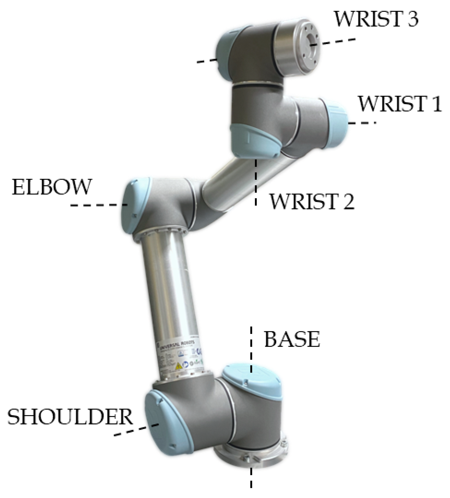
The case study faced in this work concerns the development of a high-fidelity model of the UR5 robot of Universal Robots A/S depicted in in Figure 1. The UR5 is a collaborative anthropomorphic robot with six degrees of freedom, which corresponds to the same number of revolute joints. A peculiarity of the UR5 structure is that it does not have a spherical wrist; therefore, there is no point in which the three axes of the wrist joints intersect. From an implementation point of view, the first three joints are equal to each other, as are the last three.

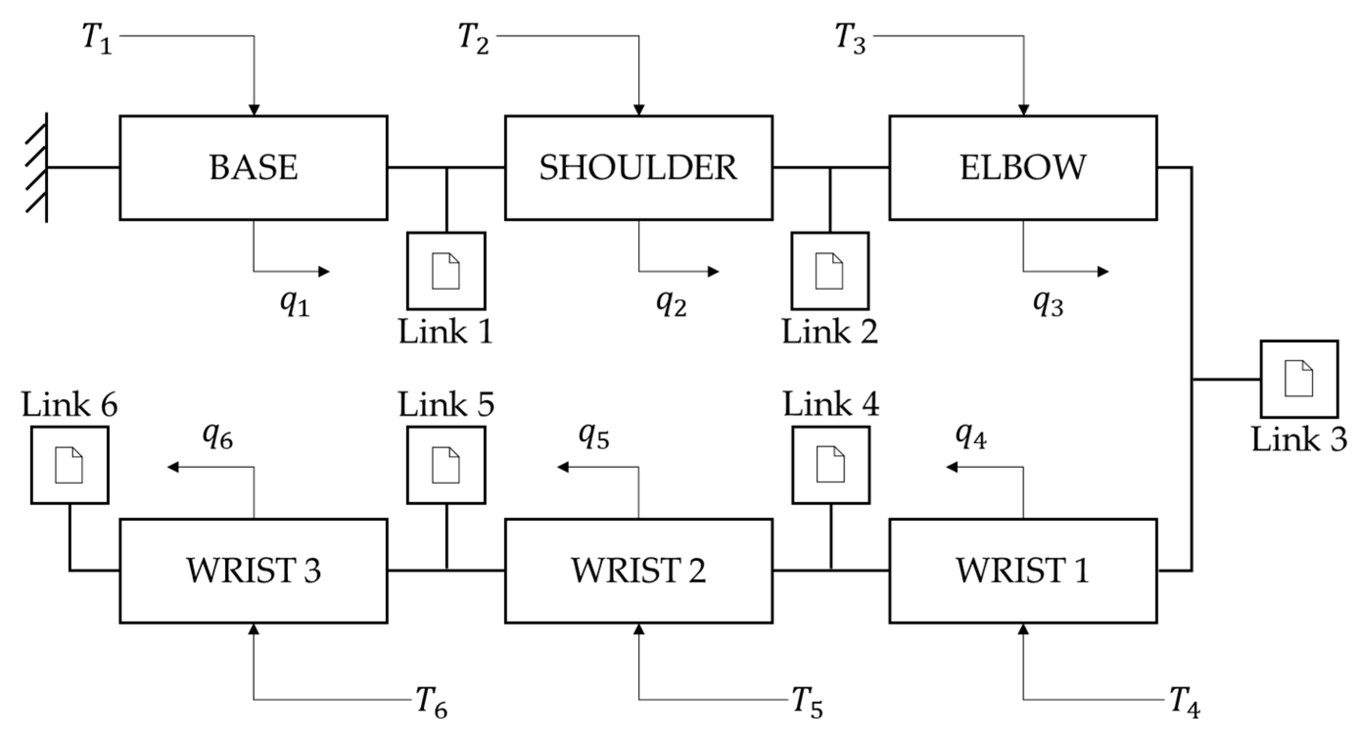
The mathematical model of the UR5 collaborative robot, whose structure is reported in Figure 2, was developed in the MATLAB-Simulink environment.

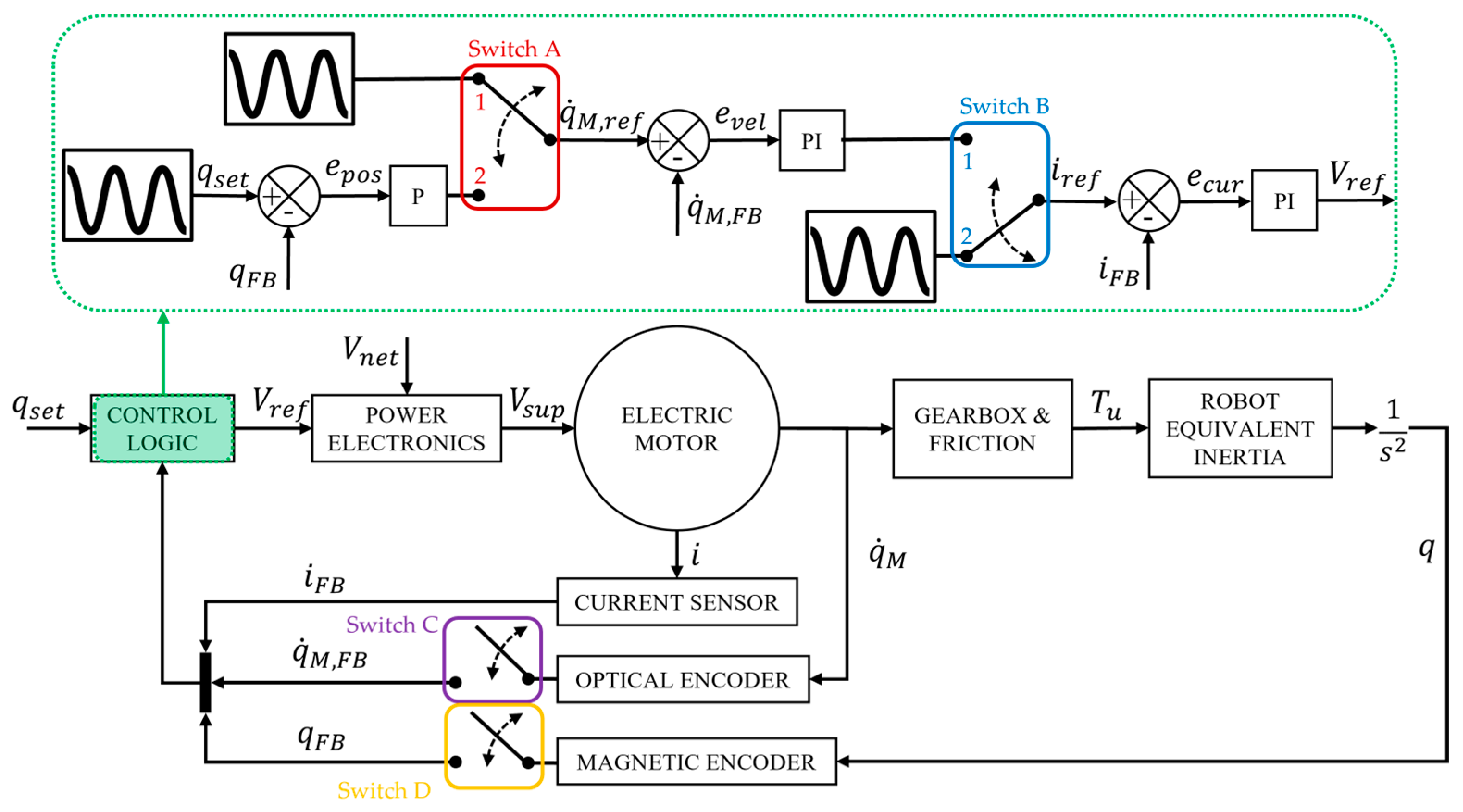
As for the real manipulator, the set of the joints’ angular positions (${\mathit{q}}_{set}=\left[q_{set,1}, q_{set,2},q_{set,3},q_{set,4},q_{set,5},q_{set,6}\right]$) is provided as input to the six joints of the robot digital replica. The main elements of each joint (e.g., control logic, power electronics, electric motor, gearbox, and sensors) were modeled by finding a good compromise between simulation time and level of detail. To simulate one second, a computer with an Intel^® i7-8750H processor at 3.91 GHz equipped with 16 GB of RAM DDR4 takes about five minutes.

For each joint, by means of three nested control loops (joint position, motor velocity, and motor current), the reference voltage ($V_{ref}$) is calculated and provided as input to the power electronics block, where, through Pulse Width Modulation (PWM), the supply voltage ($V_{sup}$) is obtained. Inside the electric motor block, the motor current ($i$) and velocity (${\dot{q}}_M$) are computed and used as inputs to the current sensor and the optical encoder, respectively, to obtain the relative feedback signals ($i_{FB}$, ${\dot{q}}_{M,FB}$). The gearbox model compares the motor and the joint angular positions and velocities ($q_M$ and $q$, ${\dot{q}}_M$ and $\dot{q}$) to calculate the reaction torque to the motor/input shaft ($T_{SWG,in}$) and the joint output torque ($T_j=T_{SWG,out}$). To this last value, the friction torque ($T_f$) is then subtracted to obtain the useful torque ($T_u$) acting on the joint shaft. The useful torques of each of the six joints of the manipulator are used in the robot arm block to solve the forward dynamics from which the joints’ angular accelerations are obtained. Once integrated, they provide the joints’ angular positions ($q$), which are given as inputs to the magnetic encoder to determine the feedback signal (${\mathit{q}}_{FB}$). Finally, through the forward kinematics of the robot arm, the pose (position and orientation) of the TCP is computed.

2.1. Control Logic and Power Electronics

Since the actual control algorithms implemented by the robot manufacturer on the real robot are unavailable, for the simulated manipulator a control logic based on proportional and integrative (PI) gains was adopted, similar to the ones proposed by [25,33]. The control parameters reported in

Table 1. Control logic parameters of the UR5 model.

Joint	Position	Velocity		Current
	P [s−1]	P [As/rad]	I [A/rad]	P [V/A]	I [V/As]
Base	7400	1	0.1	10	10,000
Shoulder	7500	1	0.2	10	10,000
Elbow	7500	0.5	0.1	30	10,000
Wrist 1	2900	0.8	0.2	30	10,000
Wrist 2	3000	1	0.2	30	10,000
Wrist 3	3250	1	0.2	30	10,000

were tuned by analyzing the frequency response function derived for each joint as described in Appendix A.

The joint control logic was structured into three nested loops. The outer one compares the desired (${\mathit{q}}_{set}$) and the feedback (${\mathit{q}}_{FB}$) signals of the joints’ angular positions to determine the position error $(e_{pos}$) of each joint. Such value is then multiplied by a proportional gain (P), to which the desired motor angular velocity (${\dot{q}}_{M,target}$) is summed to obtain the reference motor angular velocity (${\dot{q}}_{M,ref}$). This approach adds a speed feedforward branch to enhance the control capabilities, exploiting the a priori knowledge of the entire trajectory, usually known in classic robot operations. The mismatch ($e_{vel}$) between such signal (${\dot{q}}_{M,ref}$) and the feedback value (${\dot{q}}_{M,FB}$) coming from the optical encoder determines the velocity error which, once compensated, becomes the reference current signal.

The motor current control loop evaluates the reference voltage ($V_{ref}$) as a function of the mismatch ($e_{cur}$) between the reference ($i_{ref}$) and the feedback ($i_{FB}$) motor currents. This is used by the power electronics block, which regulates the network voltage ($V_{net}$= 48 V) providing the PWM supply voltage ($V_{sup}$) to the electric motors.

2.2. Electric Motor

The UR5 is equipped with six Permanent Magnets AC Synchronous Motors (PMSMs), which combine the high precision in speed control typical of a synchronous motor with the simple and robust design of an asynchronous one. To reduce the model complexity, the motors of the simulated manipulator were described through their equivalent DC monophase models receiving as input the supply voltage ($V_{sup}$) and providing, as output, the motor torque $T_M=k_{t}i$, where $k_t$ is the torque constant and $i$ is the motor current. The motor dynamics are described through two electrical and mechanical equilibrium equations:

$$\{\begin{array}{c}{V}_{sup}=L\frac{di}{dt}+Ri+k_e{\dot{q}}_M\\ J_M\frac{d{\dot{q}}_M}{dt}=k_{t}i-T_{SWG,in}\end{array},$$

(1)

where $R$ and $L$ are, respectively, the equivalent DC motor winding resistance and inductance, $k_e$ is the motor back-EMF constant, assumed, at first approximation, to be equal to $k_t$, ${\dot{q}}_M$ is the motor angular velocity, $J_M$ is the rotor inertia, and $T_{SWG,in}$ is the reaction torque generated by the reducer on the motor shaft and represents the disturbance torque to the electric motor. The values of the aforementioned parameters are provided in

Table 2. UR5 motor parameters.

Joint	${\mathit{J}}_{\mathit{M}} \left[{\mathbf{kgm}}^2\right]$	$\mathit{R} [\mathbf{\Omega }]$	$\mathit{L} \left[\mathsf{H}\right]$	${\mathit{k}}_{\mathit{t}} [\mathbf{Nm}/\mathbf{A}]$
Base, shoulder, elbow	1.877 × 10−4	0.30	0.83 × 10−3	[0.1350, 0.1361, 0.1355]
Wrist 1, Wrist 2, Wrist 3	2.076 × 10−5	1.65	2.50 × 10−3	[0.0957, 0.0865, 0.0893]

.

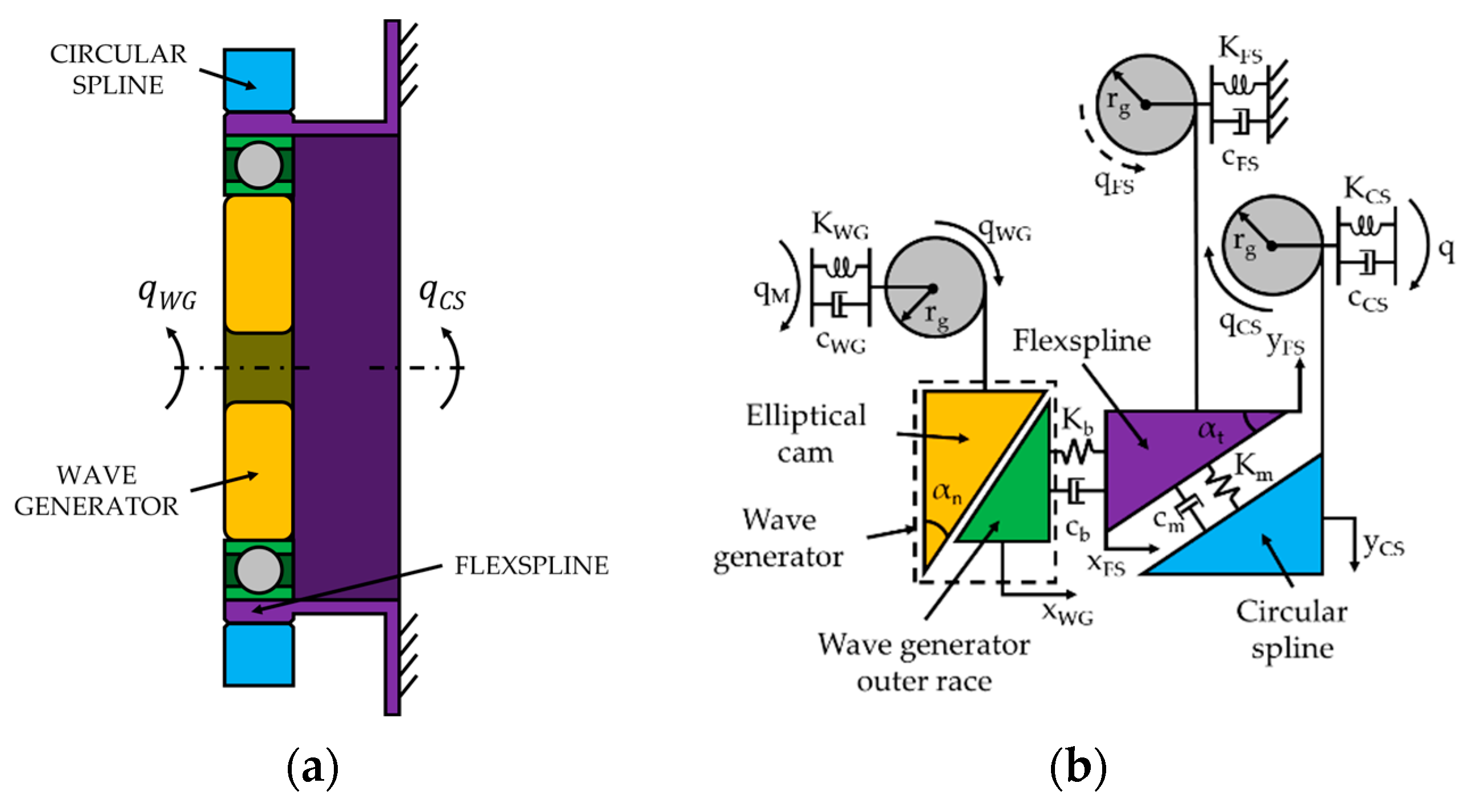
2.3. Gearbox

The Strain Wave Gear (SWG), also known as harmonic drive, is a reducer widely adopted in several industrial fields, ranging from industrial and collaborative robotics [44,45] to aerospace applications [46], due to its high reduction ratio, virtually zero-backlash, and compact and light-weight design. This gear can be functionally described through its three main components: Wave Generator (WG), Flexspline (FS), and Circular Spline (CS). The WG consists of an elliptical cam (wave generator plug) inserted in a deformable ball bearing which is then pushed inside the FS, a thin-walled gear with external toothing engaging with the CS, a rigid gear with internal toothing. The behavior of the gear changes according to the mounting configuration of these three components. As an example, for the UR5 manipulator, the input shaft is always integral to the WG, while the output one is integral to the CS, as the FS fixed to the joint case. This leads to a reduction ratio ($\tau$), defined as:

$$\tau =\frac{Z_{CS}}{Z_{CS}-Z_{FS}}$$

(2)

where $Z_{FS}$ and $Z_{CS}$ are, respectively, the number of the flexspline and the circular spline teeth. Since, for the robot under analysis, $Z_{FS}=200$ and $Z_{CS}=202$, the gear ratio reported in Equation (2) is $\tau =101$. Due to its elliptical shape, the rotation of the wave generator elastically deforms the flexspline along its major axis, allowing it to mesh with the circular spline. Since the number of FS teeth is two fewer than the one of CS, for a full rotation of the input shaft, the output one rotates of an angle corresponding to two teeth. For the proposed case study, according to Equation (2), for each 360° of rotation of the WG, the CS rotates, in the same direction, by about 3.56°.

To replicate the behavior of the strain wave gear, a translation equivalent model, based on the research in [47,48], was implemented on each joint of the UR5 manipulator. This allows describing the cyclic deformation of the flexspline and its interaction with the circular spline through equivalent tangential and radial displacements. Damping–stiffness ($c-k$) coefficients [49] were used to describe the interactions not only between the contact interfaces within the SWG, but also between the motor shaft and the WG, and between the CS and the joint output flange. Therefore, it is possible to decouple the dynamics of the SWG from those of the input and the output shafts, leading to a four-DoF model. The schematic representations of the proposed gear model is reported in Figure 3. Here, the curved continuous arrows are used to schematize the rotation of the gear elements, while the dashed ones represent their small oscillations due to their compliant connections to the joint housing represented through a damper and a torsional stiffness.

To properly describe the behavior of the gearbox, both the kinematic and dynamic parameters (e.g., inertia and torsional stiffness) of the gears were characterized. According to [50], the UR5 collaborative robot was equipped with the same joint/reducer size for the first three joints (base, shoulder, and elbow), while a smaller one is mounted on the last three (wrist 1, wrist 2, and wrist 3). For convenience, in the present document, these two sizes will be labeled as A and B, respectively, for the bigger and the smaller reducers.

The translation model of the SWG reported in Figure 3b is based on the possibility to correlate the angular quantities of the actual gear (e.g., input and output shaft rotations) to the equivalent translational ones through a primitive equivalent radius ($r_g$) equal to the undeformed FS radius. To respect the actual transmission ratio, the elliptical cam equivalent angle (${\alpha }_n$) was described as a function of the gear ratio ($\tau$) and the tooth pressure angle (${\alpha }_t$) as:

$${\alpha }_n=\arctan \left(\frac{1}{\tau \tan {\alpha }_t}\right)$$

(3)

While the inertia values of the wave generator ($J_{WG}$), the flexspline ($J_{FS}$), and the circular spline ($J_{CS}$) for the two reducers were derived from the CAD files, the torsional stiffness ($K_{WG}$, $K_{FS}$, $K_{CS}$) of the single elements of the strain wave gears were approximated using the formula for hollow cylinders:

$$K=\frac{\pi E\left(d_{ext}^4-d_{int}^4\right)}{64l\left(1+\nu \right)}$$

(4)

where $E=206\times {10}^9\mathrm{N}/{\mathrm{m}}^2$ and $\nu =0.26$ are the steel Young modulus and Poisson coefficient, $l$ is the shaft length, and $d_{ext}$ and $d_{int}$ are, respectively, the external and internal diameters of the single component. On the contrary, the linear stiffnesses used to model the contact between the WG outer race and the FS inner surface ($K_b$) and the one associated with the FS-CS teeth meshing ($K_m$) were derived from the literature [51], while all the damping factors were set equal to 0.1. The values used in the proposed model are summarized in

Table 3. Strain wave gear parameters.

Parameter	Units	Size A	Size B
$r_g$	mm	30.65	16.90
${\alpha }_t$	deg	30	30
$K_{WG}$	Nm/rad	1.92 × 105	1.77 × 104
$K_b$	N/m	1.9 × 108	1.2 × 108
$K_{FS}$	Nm/rad	3.99 × 105	7.26 × 104
$K_m$	N/m	5.70 × 108	3.20 × 108
$K_{CS}$	Nm/rad	1.98 × 107	6.23 × 106
$J_{WG}$	kgm2	2.60 × 10−5	2.21 × 10−6
$J_{FS}$	kgm2	2.65 × 10−4	3.75 × 10−5
$J_{CS}$	kgm2	2.43 × 10−4	1.85 × 10−5

.

To calculate the torque transmitted by the reducer ($T_j=T_{SWG,out}$ equal to $T_{FS}$ or $T_{CS}$, according to the gear mounting configuration), it is necessary to solve the dynamic equilibrium of the WG, the FS, and the CS schematized in Figure 3b. The equations describing the interactions among the single elements of the gear are [51]:

$$\{\begin{array}{l}{J}_{WG}{\ddot{q}}_{WG}=T_{SWG,in}-F_b{r}_g{s}_{{\alpha }_n}{c}_{{\alpha }_n}\\ \frac{J_{FS}{\ddot{x}}_{FS}}{r_g^2}=F_b-F_m{s}_{{\alpha }_t}\\ \frac{J_{FS}{\ddot{y}}_{FS}}{r_g^2}=F_m{c}_{{\alpha }_t}-F_t\\ J_{CS}{\ddot{q}}_{CS}=F_m{r}_g{c}_{{\alpha }_t}-T_{CS}\\ T_{SWG,in}=K_{WG}(q_M-q_{WG})+c_{WG}({\dot{q}}_M-{\dot{q}}_{WG})\\ F_b=K_b(x_{WG}-x_{FS})+c_b({\dot{x}}_{WG}-{\dot{x}}_{FS})\\ F_m=K_m[x_{FS}{s}_{{\alpha }_t}-(y_{CS}+y_{FS})c_{{\alpha }_t}]+c_m[{\dot{x}}_{FS}{s}_{{\alpha }_t}-({\dot{y}}_{CS}+{\dot{y}}_{FS})c_{{\alpha }_t}]\\ F_t=\frac{K_{FS}{y}_{FS}}{r_g^2}+\frac{c_{FS}{\dot{y}}_{FS}}{r_g^2}\\ T_{CS}=K_{CS}(q_{CS}-q)+c_{CS}({\dot{q}}_{CS}-\dot{q})\end{array}$$

(5)

where, for better clarity, the general notation $c_x=\cos \left(x\right)$ and $s_x=\sin \left(x\right)$ was adopted. The nine equations used to describe the kinematic and dynamic behavior of the single reducer can be classified into two groups:

• Group 1: comprised of the first four equations describing, respectively, the dynamic equilibrium of the wave generator, the flexspline radial and tangential contributions, and the one of the circular spline;
• Group 2: comprised of the last five equations, representing the interactions between the input shaft and the elliptical cam, through the WG bearing, between the FS and the CS teeth, and between the FS and the joint case and the CS with the output shaft.

To ensure the correct functioning of the proposed gear models, the initial conditions were defined according to the starting angular positions of the input/motor shafts and the output/joint shafts, obtained from the solution of the following set of equations:

$$\left[\begin{array}{cccccc}{K}_{WG}& K_b{r}_g{s}_{{\alpha }_n}{c}_{{\alpha }_n}& -K_b{r}_g{s}_{{\alpha }_n}{c}_{{\alpha }_n}& 0& 0& 0\\ 0& K_b& -(K_b+K_m{s}_{{\alpha }_t}^2)& K_m{s}_{{\alpha }_t}{c}_{{\alpha }_t}& K_m{s}_{{\alpha }_t}{c}_{{\alpha }_t}& 0\\ 0& 0& -K_m{s}_{{\alpha }_t}{c}_{{\alpha }_t}& K_m{c}_{{\alpha }_t}^2+\frac{K_{FS}}{r_g^2}& K_m{c}_{{\alpha }_t}^2& 0\\ 0& 0& -K_m{r}_g{s}_{{\alpha }_t}{c}_{{\alpha }_t}& K_m{r}_g{c}_{{\alpha }_t}^2& K_m{r}_g{c}_{{\alpha }_t}^2& K_{CS}\\ r_g\tan {\alpha }_n& -1& 0& 0& 0& 0\\ 0& 0& 0& 0& -1& r_g\end{array}\right]\left(\begin{array}{c}{q}_{WG,0}\\ x_{WG,0}\\ x_{FS,0}\\ y_{FS,0}\\ y_{CS,0}\\ q_{CS,0}\end{array}\right)=\left(\begin{array}{c}{K}_{WG}{q}_{M,0}\\ 0\\ 0\\ K_{CS}{q}_0\\ 0\\ 0\end{array}\right)$$

(6)

2.4. Friction

In contrast with [48], friction was not implemented at the single contact interfaces of the SWG, but defined as an overall joint friction torque. This was chosen to implement the Coulomb ($f_c$) and the viscous ($f_v$) friction coefficients derived through the base dynamic parameters identification process in the proposed robot model, as described in [52]. However, the friction model used to build the regression matrix in [40] does not properly replicate the actual trend of a joint friction. To describe the behavior associated with the input and output bearings inside the robot joint, the Stribeck curve proposed in [53] was modified in the one reported in Equation (7) through the exponent associated with the joint angular velocity ($\dot{q}$) [51]. The friction torque $T_f$ between the input and output of each joint was modeled through the interaction of the LuGre elastic bristles as proposed in [54], leading to:

$$\{\begin{array}{l}{T}_f={\sigma }_{0}z+{\sigma }_1\dot{z}\hfill \\ \dot{z}=\dot{q}-\frac{\left|\dot{q}\right|z}{g\left(\dot{q}\right)}{\sigma }_0\hfill \\ g\left(\dot{q}\right)=f_c\left(1+K_{static}{e}^{\frac{-k_q\left|\dot{q}\right|}{\left|{\dot{q}}_s\right|}}\right)+f_v{\dot{q}}^{\raisebox{1ex}{$2$}\!\left/ \!\raisebox{-1ex}{$3$}\right.}\hfill \end{array}$$

(7)

where ${\sigma }_0=5\times {10}^6 \mathrm{Nm}/\mathrm{rad}$ and ${\sigma }_1=100 \mathrm{Nms}/\mathrm{rad}$ are, respectively, the stiffness and the damping coefficient of the bristles subjected to an average deflection $z$ at a speed $\dot{z}$, $\dot{q}$ is the joint angular velocity (equal to the relative velocity of the two contact surfaces), $g\left(\dot{q}\right)$ also depends on surface materials, lubrication regime, and temperature, ${\dot{q}}_s=0.5 \mathrm{rad}/\mathrm{s}$ is the sliding speed threshold used to describe the Stribeck effect, $K_{static}=0.3$ is the static friction increment with respect to the Coulomb friction $f_c$ which leads to the stiction friction force, while $k_q$ and $f_v$ are the Stribeck parameter and the viscous friction coefficient, respectively, selected in order to reproduce the experimental behavior [52]. Other possible formulations of the friction curve for a robot joint can be found in [55,56]. The LuGre model allows considering micro-displacements, which are represented with a spring-like behavior.

2.5. Sensors

According to the scheme reported in Figure 2, each joint of the robot was equipped with three sensors:

• Optical encoder: an encoder integral to the motor/input shaft used to derive the motor angular velocity (${\dot{q}}_M$) used to provide the feedback signal (${\dot{q}}_{M,FB}$) to the velocity control loop;
• Magnetic encoder: an encoder integral to the joint/output shaft used to measure the joint actual angular position ($q$) used to close the position control loop through the feedback signal ($q_{FB}$);
• Current sensor: used to measure the motor current ($i$) necessary to close the current control loop through the feedback signal ($i_{FB}$).

Such sensors were modeled using first-order transfer functions for the current sensors, while second-order ones were implemented for both input and output encoders. For a more realistic description of the real sensors, noise was added to the feedback signals, which were then digitalized by means of a sample and hold circuit and a quantizer. The noise standard deviation was the same as the one measured from the UR5.

Moreover, in the real robot, each joint is also equipped with a thermocouple used to measure the joint temperature. However, since heat transfer was neglected in the proposed joint model, this sensor was not implemented.

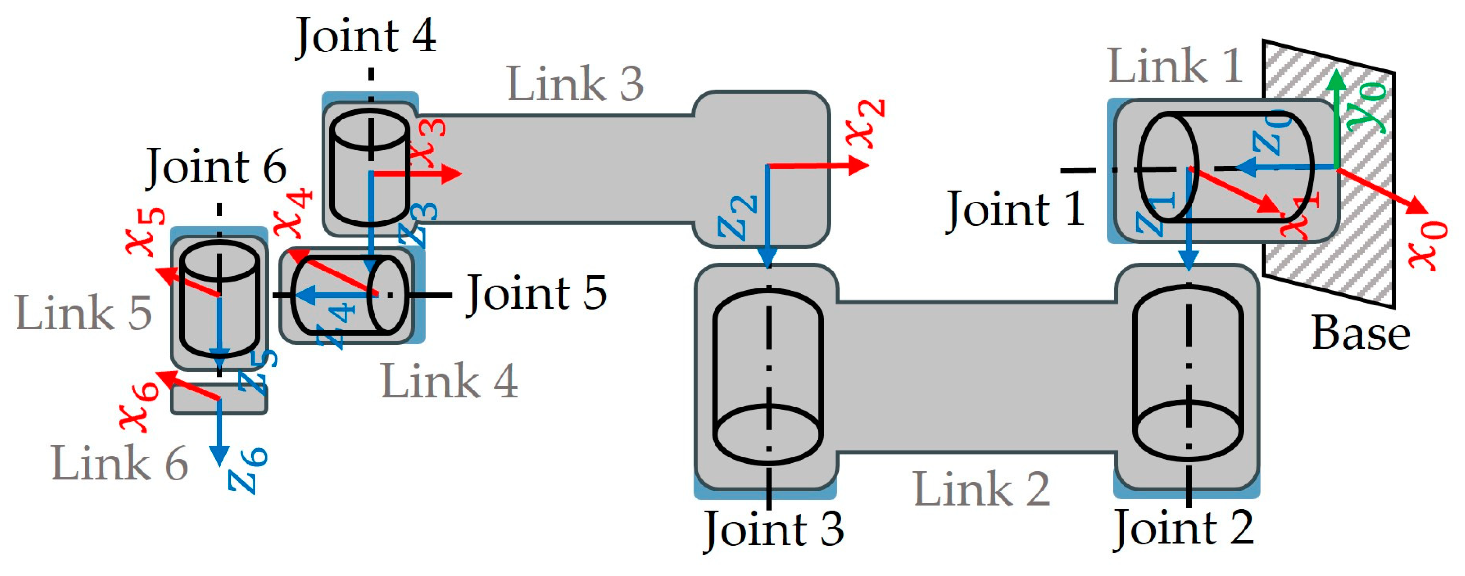
2.6. Six-DoF Forward Kinematics and Dynamics

The robot arm subsystem, shown in Figure 2, contains the Simscape Multibody model with which the single joints and links of the UR5 digital replica are connected, as depicted in Figure 4.

The relative position and orientation of the joint reference frame $i$ with respect to the previous one $i-1$ are described through the 4 × 4 roto-translation matrix ⁱ⁻¹A_i as:

$$\begin{array}{cc}& {}^{i-1}{\mathit{A}}_i=\mathrm{Transl}(z_i,d_i)·\mathrm{Rot}(z_i,{\theta }_i)·\mathrm{Transl}(x_i,a_i)·\mathrm{Rot}(x_i,{\alpha }_i)·\mathrm{Rot}(y_i,{\beta }_i)\\ & {}^{i-1}{\mathit{A}}_i=\left[\begin{array}{cccc}{c}_{{\theta }_i}{c}_{{\beta }_i}-s_{{\theta }_i}{s}_{{\alpha }_i}{s}_{{\beta }_i}& -s_{{\theta }_i}{c}_{{\alpha }_i}& c_{{\theta }_i}{s}_{{\beta }_i}+s_{{\theta }_i}{s}_{{\alpha }_i}{c}_{{\beta }_i}& a_i{c}_{{\theta }_i}\\ s_{{\theta }_i}{c}_{{\beta }_i}+c_{{\theta }_i}{s}_{{\alpha }_i}{s}_{{\beta }_i}& c_{{\theta }_i}{c}_{{\alpha }_i}& s_{{\theta }_i}{s}_{{\beta }_i}-c_{{\theta }_i}{s}_{{\alpha }_i}{c}_{{\beta }_i}& a_i{s}_{{\theta }_i}\\ -c_{{\alpha }_i}{s}_{{\beta }_i}& s_{{\alpha }_i}& c_{{\alpha }_i}{c}_{{\beta }_i}& d_i\\ 0& 0& 0& 1\end{array}\right]\end{array}$$

(8)

As in Section 2.3, for better clarity, the general notation $c_x=\cos \left(x\right)$ and $s_x=\sin \left(x\right)$ was adopted. The values of the variables in Equation (8) were obtained through post-processing of the ones derived from the dual robot calibration performed by the manufacturer [57]. Nominally, each UR5 collaborative robot is geometrically described by the Denavit–Hartenberg (DH) parameters provided in [58]. However, due to production tolerances and mounting errors, it is necessary to calibrate each robot to achieve the desired position accuracy and repeatability. According to [59], through the DH convention, for links between two nearly parallel joints, it is not possible to obtain, after the calibration process, corrections to the robot geometric parameters with a physical meaning. In the proposed use case, for example, the values of the DH parameter $d$ for links 2 and 3 have an order of magnitude of kilometers. To avoid using unrealistic numbers, it was necessary to merge the Denavit–Hartemberg convention with the one proposed by Hayati in [59], leading to the roto-translation matrix shown in Equation (8) and to the kinematic parameters reported in

Table 4. Kinematic parameters of the UR5 after calibration.

Link	$\mathit{a}$ [mm]	$\mathit{\alpha }$ [°]	$\mathit{\beta }$ [°]	$\mathit{d}$ [mm]	$\mathit{\theta }$ [°]
Link 1	0.110	89.905	0	89.084	0.003
Link 2	−425.156	0.004	0.013	0	−0.019
Link 3	−392.066	−0.232	0.071	0	−0.013
Link 4	0.025	89.966	0	110.212	−0.008
Link 5	−0.069	−90.013	0	94.879	0.009
Link 6	0	0	0	82.494	−0.006

.

To complete the description of the robot arm, the dynamic properties reported in

Table 5. Dynamic parameters of the UR5 [58,60].

Link	Mass [kg]	Center of Mass [x, y, z] [m]	Inertia Tensor [Ixx, Iyy, Izz, Ixy = Iyx, Ixz = Izx, Iyz = Izzy] [kgm2]
Link 1	3.7	[0, −0.02561, 0.00193]	[67, 64, 67, 0, 0, 0]
Link 2	8.393	[0.2125, 0, 0.11336]	[149, 3564, 3553, 0, 0, 0] × 10−4
Link 3	2.33	[0.15, 0, 0.0265]	[25, 551, 546, 0, 34, 0] × 10−4
Link 4	1.219	[0, −0.0018, 0.01634]	[12, 12, 9, 0, 0, 0] × 10−4
Link 5	1.219	[0, 0.0018, 0.01634]	[12, 12, 9, 0, 0, 0] × 10−4
Link 6	0.1879	[0, 0, −0.001159]	[1, 1, 1, 0, 0, 0] × 10−4

were associated with the single links of the manipulator.

From a dynamic point of view, the description of the behavior of the manipulator was obtained by exploiting the Simulink/Simscape environment. Within it, a casual object-oriented programming language, individual system model, and its interconnections describe the underlying dynamics equation. This approach allows the design of the model to be based on the actual structure of the physical system. The kinematic and dynamic parameters reported in Table 4 and Table 5 were used to build the multibody Simscape model schematized in Figure 5.

As shown in Figure 2, each joint $j$ sub-model receives as input the torque ($T_j$) provided by the reducer and calculated through Equation (5). As an output, each block provides the joint angular position ($q_j$). Within the sub model of each joint, mass, Coriolis, and gravity matrices are automatically constructed, while the friction matrix is provided by exploiting the LuGre model as illustrated in Section 2.4, to compute the direct dynamics of the manipulator.

3. Experimental Testing

To examine the goodness of the proposed model, several trajectories were applied to both the UR5 and its digital replica. As an example, in the present paper, two different test trajectories were analyzed. On one hand, specific movements designed to properly excite the robot dynamic parameters, such as the ones reported in [26,61,62], were provided as inputs to evaluate the ability of the proposed model to replicate a high-dynamic behavior of the real robot. 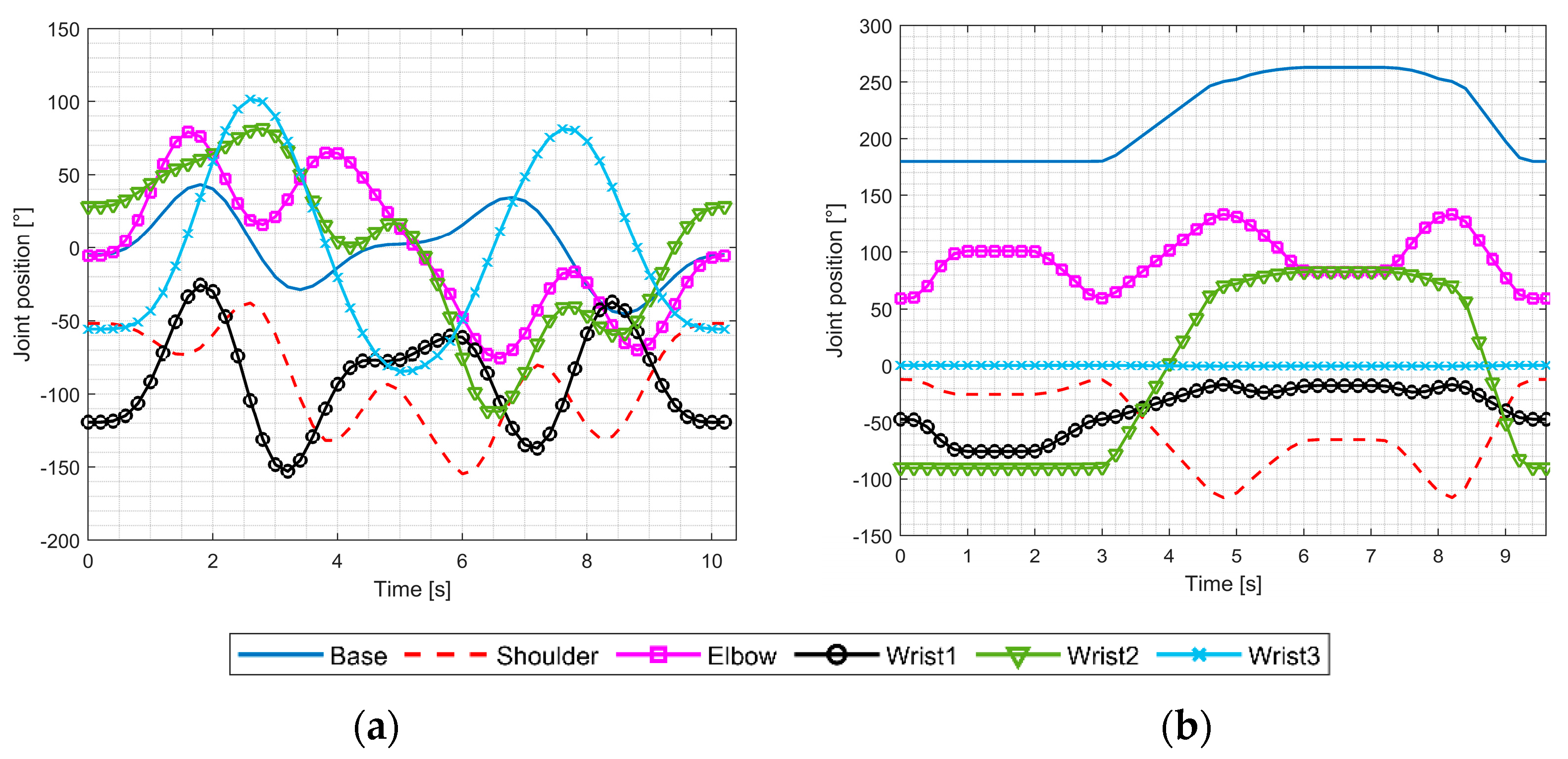On the other hand, since, according to [63], pick-and-place is the most common application for both industrial and collaborative robots, the model performance was also evaluated with a trajectory representative of such movements. In both cases, the desired joints’ angular positions of the test trajectories, reported in Figure 6, were applied to the UR5 through port 29999 [64], while the joints’ angular positions and velocities and the motors’ current signals were acquired at a frequency of 125 Hz using port 30003.

For both trajectories, to clearly plot the joints’ torques and to improve the paper readability, the current signals were filtered with a low-pass filter at a cutoff frequency of 10 Hz. On the contrary, no filtering was required for the joints’ angular positions.

3.1. Dynamic Parameters Excitation Trajectory

Due to the complexity of such excitation trajectory, to move the real manipulator, the robot built-in function servoj (target joint configuration, acceleration, velocity, time, lookahead time, gain) was adopted [65]. The numerical values of acceleration, velocity, time, lookahead time, and gain were set equal to 0 rad/s², 0 rad/s, 0.08 ms, 0.03, and 500, respectively.

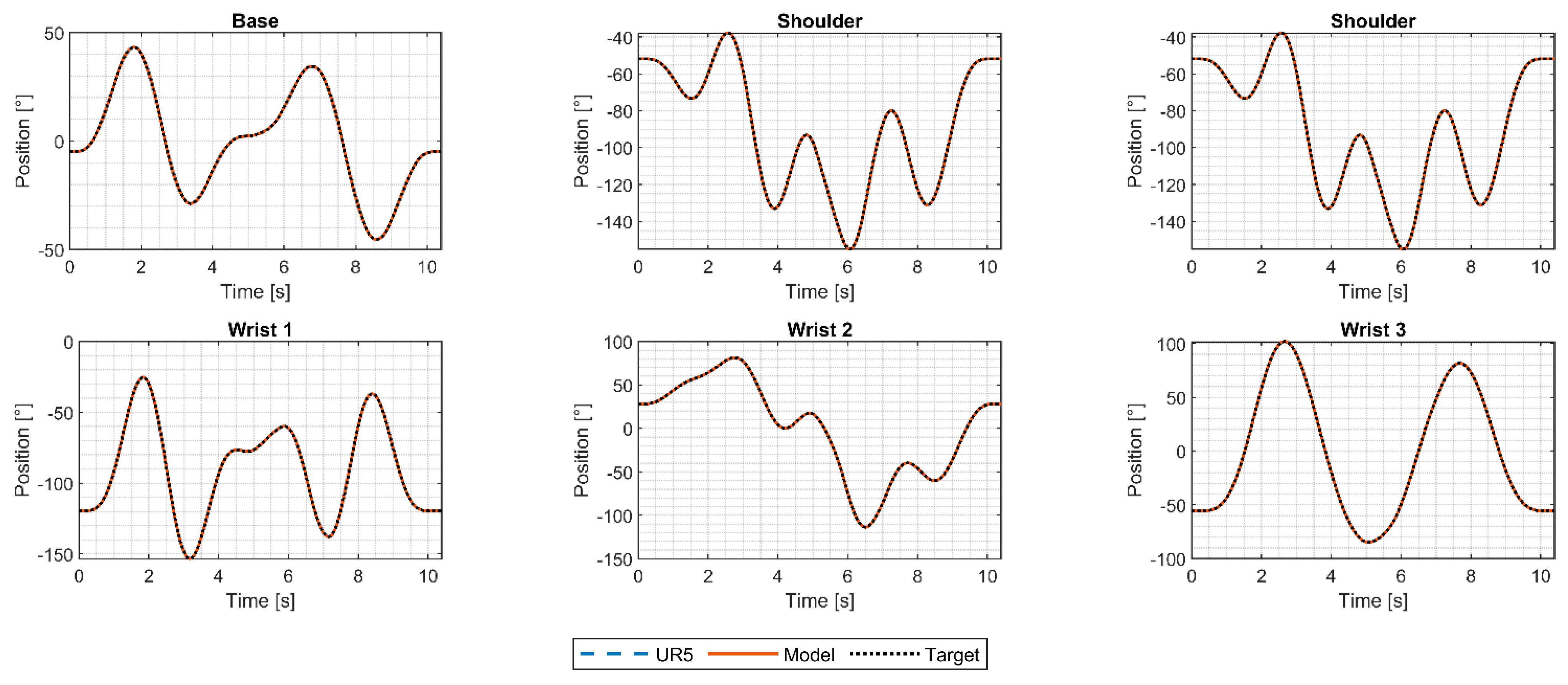
The ability of the proposed model to follow the desired trajectory can be seen in Figure 7, where both set and feedback joints’ angular position signals are reported.

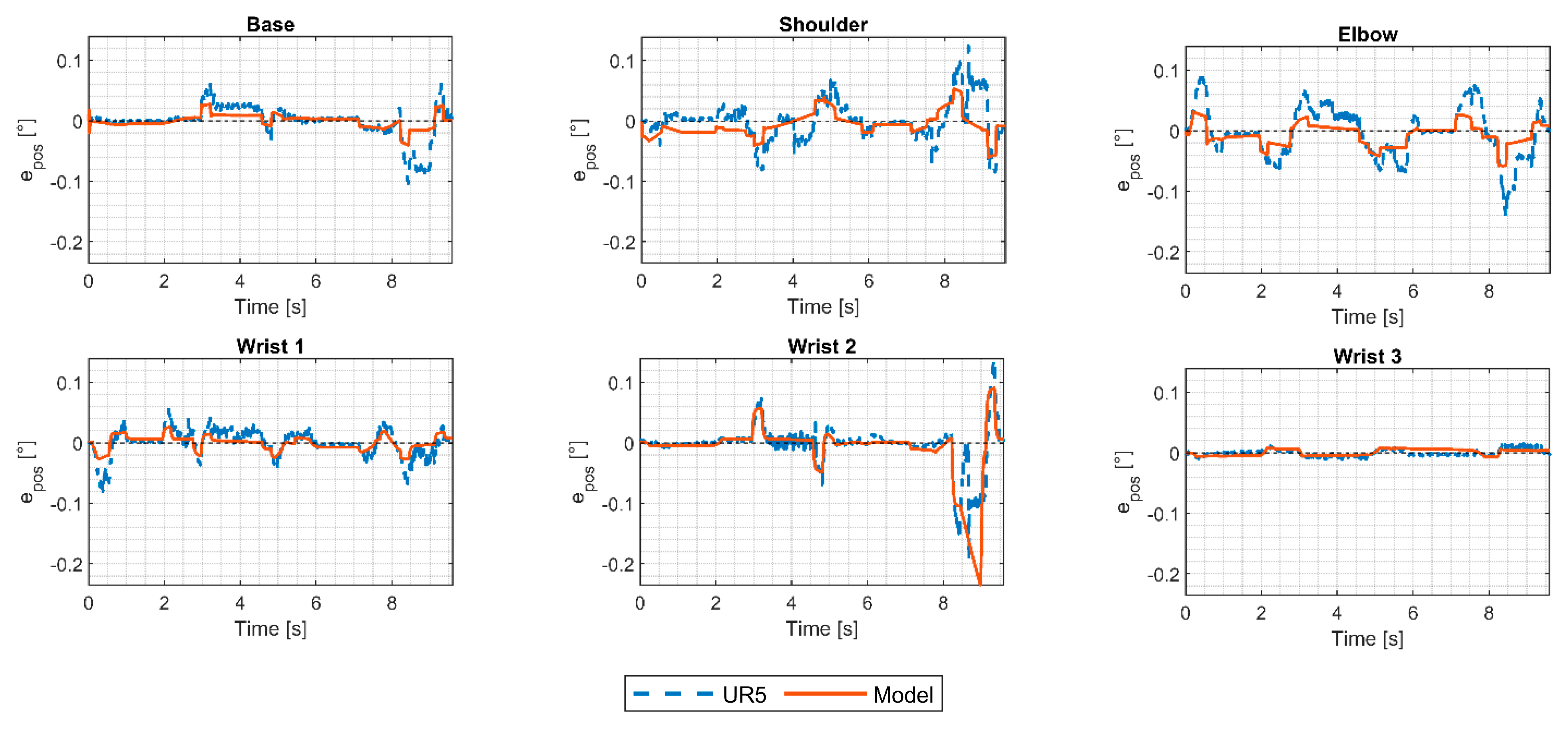
Since, for all the joints, the trends of the three curves well overlap, Figure 8 reports the mismatches between such set and feedback signals to better highlight the tracking error of both the real and the simulated robots. For better comparison, the axes scales are the same for all the joint plots.

By analyzing the position errors for each joint, it can be seen that they not only have the same order of magnitude for both manipulators, but they also share similar trends, proving that the proposed model is able to replicate the actual behavior of the real UR5. It should be also noticed that the position error of the proposed model is lower than that of the real robot, with a maximum value of about 0.08°. However, the apparent better performance of the proposed model is likely related to the simplifications adopted. Among all, the strain wave gear torsional hysteresis [66] was not modeled in the translation equivalent model of the strain wave gear of Figure 3. Such a simplification leads to the gears always having the same torsional stiffness during the entire trajectory, while studies in the literature [67,68] showed that this is a function of the applied torque. This, together with the approximations of the gear stiffness values, might lead the digital replica to be stiffer than the real robot, allowing its control logic to better compensate for position errors.

Nevertheless, the low tracking errors between the set and feedback joints’ angular positions translate into an actual path of the TCP close to the ideal/desired one, which is of paramount importance for applications such as welding, dispensing, and gluing. The position and the orientation of the robot TCP with respect to the fixed base reference frame (⁰A₆), in fact, are described by the combination of rigid body transformation matrices described in Equation (8) for each joint as:

$${}_{ }{}^0\mathit{A}{}_6=\prod _{i=0}^5{}_{ }{}^{i}A{}_{i+1}$$

(9)

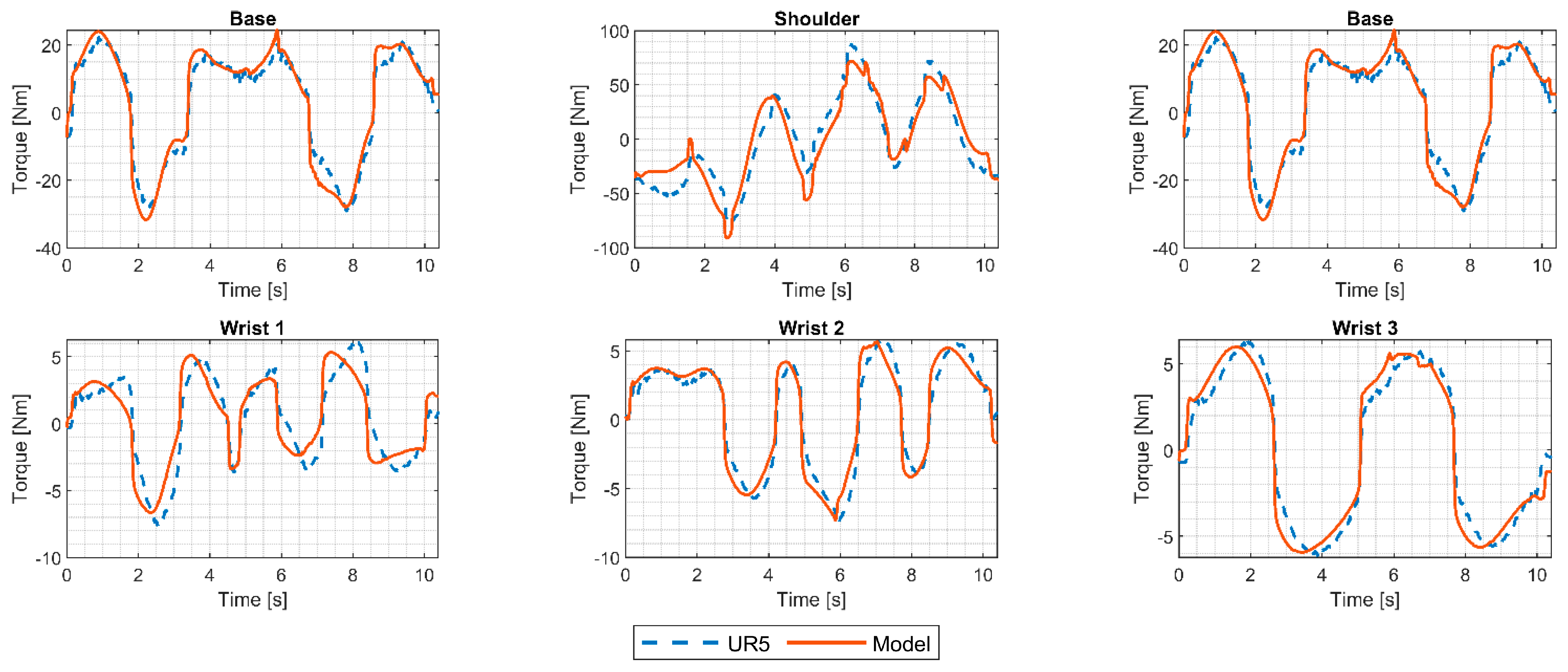
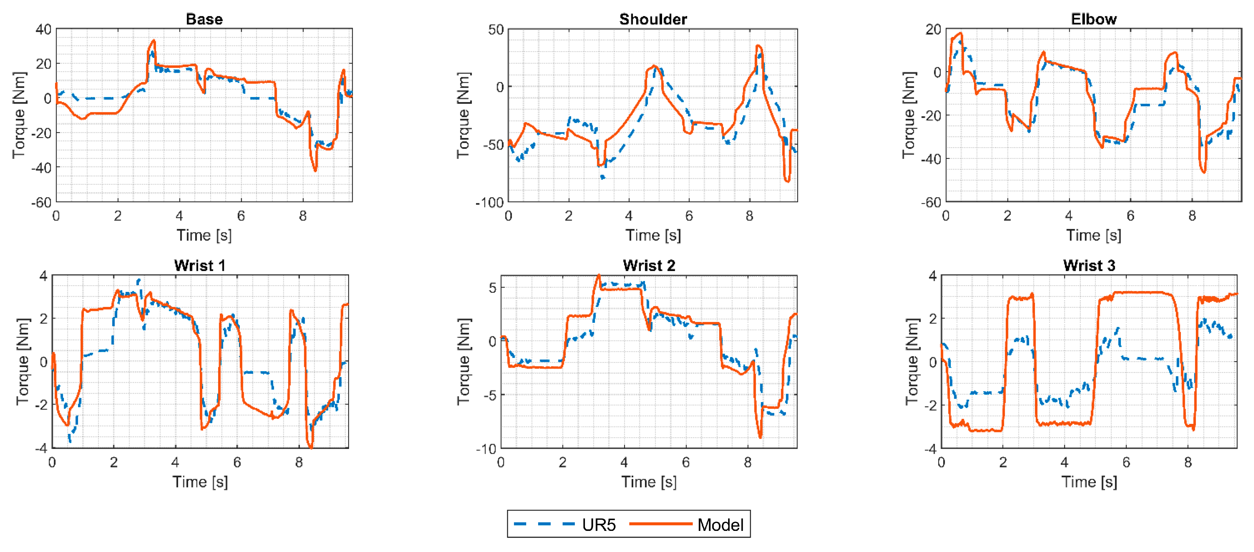
According to the control logic reported in Figure 2, the position error was used to compute the target/reference motor angular velocity whose difference with the feedback signal, once compensated, provides the motor current for each joint. By multiplying the feedback currents (${\mathit{i}}_{FB}$) by the reduction ratio ($\tau$) and the motor torque constants ($k_t$) reported in Table 2, the joint reducer output torques of the two manipulators are derived and compared in Figure 9.

Even though the simulated torques (Model) well approximate the measured ones (UR5), some intervals of the tested trajectory show higher mismatches between the two sets of data. Such a residual difference might be related to several causes, such as:

• Implementation of simplified DC models of the joint motors instead of using three-phase ones, whose parameters, such as resistance and inductance, are not fully known. Moreover, the motor back-EMF constant ($k_e$) was assumed to be constant for the entire trajectory, while it slightly changes with the applied load.
• A possible incorrect description of the joint friction. As already mentioned, the identification algorithms provided by [40,52] only take into account viscous and Coulomb friction, while they are not able to describe more complex trends, such as the ones affecting the real robot. To do so, friction was modeled through Equation (7), whose coefficients were tuned according to several experimental campaigns aiming to reach a good overall fit between simulated and measured motor currents.
• Lack of both the kinematic error and the gear torsional hysteresis in the translation-equivalent models of the strain wave gears.
• The joint control logic schematized in Figure 2 is not the same as the one implemented in the real robot, which is unknown. As an example, studies such as [69,70] highlight how manipulators from Universal Robots are equipped with vibration suppression algorithms, which were not implemented in the current model. Having two different control logics deeply affects the torque trends. Since, according to the scheme reported in Figure 2, the current control loop is the most internal one, the reference value of the motor current is affected by both the position and the velocity control loops. As a direct consequence, since, as depicted in Figure 8, the joint position error is different between the two manipulators, the velocity reference signal will also be different. Hence, based on the adopted PI gains, the motor angular velocity error differs from the one of the real robot as well.
• While the control parameters reported in Table 1 are constant, it should not be excluded that Universal Robots A/S might adopt variable settings according to the specific operating conditions of the manipulator. such as very fast or very slow movements.

All the aforementioned major simplifications adopted in the present work increase the difficulty of building a digital shadow of the UR5 able to replicate the actual joint torques. More accurate estimates could be reached with a more detailed model of the single components of the robot arm, but this would negatively affect the computational cost of the robot digital replica, leading to simulation times high enough to nullify the advantage of higher precision in describing the actual dynamic behavior of the manipulator. Nevertheless, the obtained results on the torque signals are quite representative of the real behavior and constitute an innovation with respect to the usually employed literature models, in which a much lighter description of the internal quantities of the robot is present.

3.2. Pick-and-Place Trajectory

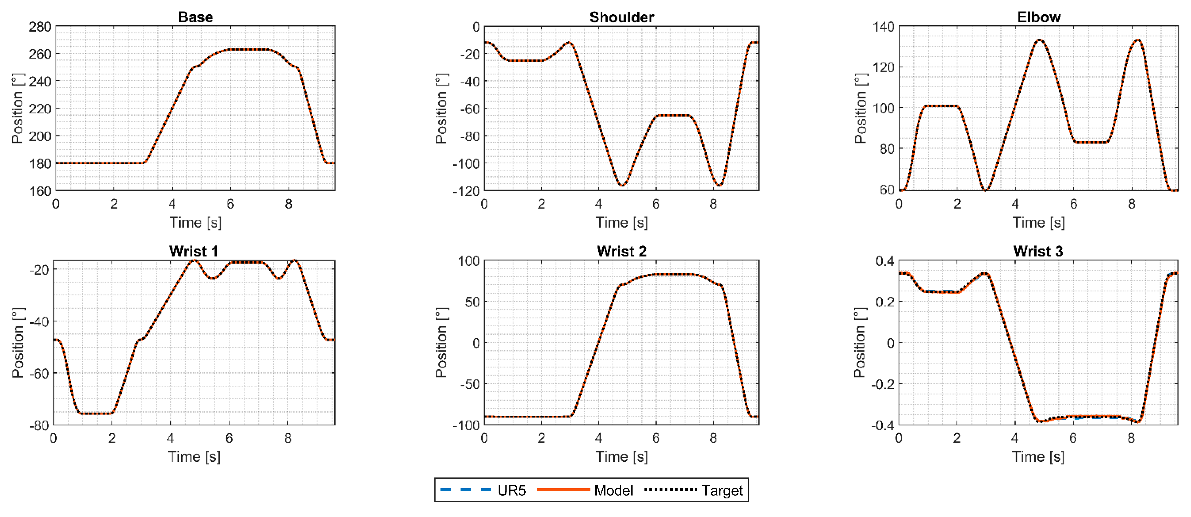
In contrast with the previous trajectory, the pick-and-place trajectory was obtained using the movel and movej commands [65] with different settings of speed and acceleration using the Polyscope programming interface on the robot teach pendant. An analysis, similar to the one reported in Section 3.1 for the dynamic parameters identification trajectory, was also conducted for the pick-and-place trajectory. The results are reported in Figure 10, Figure 11 and Figure 12.

By comparing Figure 11 with Figure 8, it can be seen that, on average, the joints’ angular positions errors are lower for the pick-and-place trajectory. This is most likely related to the lower dynamics involved in this task with respect to the rapid and continuously changing movements required to identify the UR5 base dynamic parameters.

The lower angular velocities involved during the pick-and-place give more time to the joint control logic to compensate for a mismatch between the desired and actual joint positions. This is particularly true for the last joint, which rotates a few tenths of degrees just to maintain the desired orientation of the TCP.

However, a position error of approximately 0.24°, about 0.05° higher than the one of the UR5, is visible at about 8.5 s in the second wrist. This is caused by a rapid deceleration of the joint from a speed of 180°/s to 0 in a short interval. In so doing, the control logic is required to rapidly adjust its target from keeping the joint at its highest rotation speed to break it according to a trapezoidal velocity trend. This rapid change generates a current spike, visible in the torque peak in Figure 12.

For the tested trajectory, the shoulder joint was affected by the highest errors. However, it should be noted that it was also the most loaded joint and its dynamics are directly affected by those of the other four following joints. It should be pointed out that, while, as shown in Figure 9, there is a good match between the measured and the simulated torques of the last joint (wrist 3), the same is not demonstrated for the pick-and-place trajectory in Figure 12. The difference in the two trends is probably caused by the possible different control logic adopted by Universal Robots A/S to handle very low movements, which would lead to extremely low angular velocity errors, as in the proposed case study where the maximum error between reference and feedback speed for all the joints is about 0.2°/s over the entire trajectory. In this scenario, the joint is almost still, but since the velocity error, even if low, is still present, it generates a current signal which is proportional to such error.

4. Conclusions

The present paper describes a high-fidelity dynamic model of a UR5 collaborative robot where the main components of robot joints were described in a detailed and physically representative way. Testing trajectories of different types were applied to both the real robot and its digital replica, showing a good match between experimental and simulated signals in terms of position, speed, and joint torques. In particular, the latter information represents the innovation with respect to a dynamic literature model, which usually disregards the dynamics of the joint electric drives.

Future work will be focused on simulating the presence of faults and failures of different origins and magnitudes to evaluate their impact on the overall behavior of the manipulator. The digital replica of the real robot will be used as a virtual test bench to generate a dataset of nominal and degraded responses, paving the way for a more detailed and thorough model-based PHM investigation. In addition, the proposed model of the strain wave gear will be improved to take into account additional dynamic effects, such as the kinematic error, the load-dependent torsional stiffness, and its relative degradation in time, due to an in-depth analysis of the internal interactions among the gear’s constitutive elements.