Article

Process of Learning from Demonstration with Paraconsistent Artificial Neural Cells for Application in Linear Cartesian Robots

by
João Inácio Da Silva Filho
1,*,
Cláudio Luís Magalhães Fernandes
1,2,
Rodrigo Silvério da Silveira
2,
Paulino Machado Gomes
2,
Sérgio Luiz da Conceição Matos
2,
Leonardo do Espirito Santo
2,
Vander Célio Nunes
2,
Hyghor Miranda Côrtes
1,
William Aparecido Celestino Lopes
2,3,
Mauricio Conceição Mario
1,4,
Dorotéa Vilanova Garcia
1,4,
Cláudio Rodrigo Torres
4,
Jair Minoro Abe
3 and
Germano Lambert-Torres
1,5,*
1
Laboratory of Applied Paraconsistent Logic, Santa Cecilia University—UNISANTA, Oswaldo Cruz Street 288, Santos 11045-907, SP, Brazil
2
National Service of Industrial Learning—Senai, SBN-Quadra 1-Bloco C Ed. Roberto Simonsen, Brasilia 71200-030, DF, Brazil
3
Graduate Program in Production Engineering, Paulista University, José Maria Whitaker Avenue, 320, São Paulo 04057-000, SP, Brazil
4
Post Graduation Program in Management and Technology in Productive Systems, Paula Souza State Center for Technological Education (CEETEPS), Bandeirantes Street, 169, São Paulo 01124-010, SP, Brazil
5
Gnarus Institute, Itajuba 37500-052, MG, Brazil
*
Authors to whom correspondence should be addressed.
Robotics 2023, 12(3), 69; https://doi.org/10.3390/robotics12030069
Submission received: 6 April 2023 / Revised: 29 April 2023 / Accepted: 4 May 2023 / Published: 6 May 2023
(This article belongs to the Section AI in Robotics)

Abstract

:
Paraconsistent Annotated Logic (PAL) is a type of non-classical logic based on concepts that allow, under certain conditions, for one to accept contradictions without invalidating conclusions. The Paraconsistent Artificial Neural Cell of Learning (lPANCell) algorithm was created from PAL-based equations. With its procedures for learning discrete patterns being represented by values contained in the closed interval between 0 and 1, the lPANCell algorithm presents responses similar to those of nonlinear dynamical systems. In this work, several tests were carried out to validate the operation of the lPANCell algorithm in a learning from demonstration (LfD) framework applied to a linear Cartesian robot (gantry robot), which was moving rectangular metallic workpieces. For the LfD process used in the teaching of trajectories in the x and y axes of the linear Cartesian robot, a Paraconsistent Artificial Neural Network (lPANnet) was built, which was composed of eight lPANCells. The results showed that lPANnet has dynamic properties with a robustness to disturbances, both in the learning process by demonstration, as well as in the imitation process. Based on this work, paraconsistent artificial neural networks of a greater complexity, which are composed of lPANCells, can be formed. This study will provide a strong contribution to research regarding learning from demonstration frameworks being applied in robotics.

1. Introduction

Innovation in the field of automation requires research into the area of artificial intelligence, which includes other sub-areas to be studied in their individual or correlated forms. Among these, we can cite research that is aimed at making machines more independent from programming processes through expert systems, autonomous robotics, and machine learning [1,2,3]. In this context, this article shows new alternatives in automation control that require machine learning to add a higher level of efficiency by implementing algorithmic structures based on paraconsistent logic—PL [4,5,6].
Classical logic is based on strictly binary principles, and in some situations where information is incomplete, contradictory, or redundant, the uncertainties contained in the data can make its application impossible. To achieve results in the research dealing with these new technologies, many works related to the study and application of non-classical logics have aroused interest within specialists in the field of industrial automation [4,5,6]. In recent years, fuzzy logic has stood out in the research involving automation. However, there are other non-classical logics that were created to be used in conditions in which classical logic, with its binary principles, proves to be inoperative. Currently, paraconsistent logic (PL), which is based on opposing the principle of non-contradiction (which is one of the basic principles of classical logic), has stood out in applications of its algorithms in various areas of knowledge [6,7].
Learning from demonstration (LfD) consists of making a machine perform new tasks, imitating procedures that are shown to it without the need for a reconfiguration or reprogramming of its software [2]. The research related to the application of this technique aims to find efficient ways in which to replace the manual programming work of machine activities by an automatic programming process, one that is exclusively conducted to repeat the task demonstrated by an expert [8,9]. As seen in [10], in the fundamental concepts of LfD usage in robotics area, there is a problem of imitation as an entity tries to produce a behavior similar to another entity [9,10]. Thus, a Tutor evolving in a world realizes an observation Ω of this world. The Tutor can perform a set of actions A (A could be empty) and follows a policy πtutor that associates to any world state a particular action. It is assumed that the optimal policy to satisfy the Tutor is:
πtutor: Ω → a ∈ A.
The Learner disposes of a set of observations O (named observation space) about the world and its own set of actions B.
The Learner follows another policy πlearner in order to produce a behavior similar to the observed one, therefore
πlearner: O → b ∈ B, πlearner ≡ πtutor.
Due to the condition that the Tutor and the system are involved in the same world, there is a perception equivalence problem in LfD.
Since the interaction between the Tutor and the system takes place in the real world, information is obtained by each of the actors through different means.
The world is observed by the system through sensors, whereas the human observes it through its own senses. In this way, the Tutor demonstrating a particular behavior can observe modifications of the world that the Learner cannot perceive. Therefore, with the comparisons of information data between the Tutor and the system contaminated with contradictions, thus generating uncertainties in the conclusions, the LfD process can reach a low level of efficiency [10,11].
Considering the conditions in which the LfD processes operate, the application of PL, which has the property of supporting contradictory information, can alleviate some problems related to this technique. In this paper we present the application of the Paraconsistent Artificial Neural Cell (lPANCell) algorithm based on Paraconsistent Annotated Logic (PAL) integrated with the learning from demonstration process (LfD) [12,13,14].

1.1. Related Works

The presentation of task models in such a way that a robot is able to learn from demonstration (LfD)—that is, without the need for new programming—is a challenge for the field of robotics engineering. Several published articles bring results from research on learning from demonstration (LfD), which aims to transfer task models to a robot through demonstration. For example, in [8] the authors present several LfD approaches to allow a robot to learn and to generalize complex tasks from demonstrations.
In this article, we show a way that enables the learning of complex trajectories with complex sets of states, which the Cartesian robot needs to reach in a certain sequence to accomplish a task. Among the works related to the approach we developed in this research, we can highlight the studies presented in [15,16,17,18,19], where the authors present approaches in which robots learn task models through interaction with human tutors, and which could identify the aim simply as a difference between the initial and final states. In other approaches, as seen in [20], the task model includes not only the objective, but also a set of ordering constraints between actions.
Other important works in the LfD process present classical artificial intelligence (AI) techniques for knowledge representation, planning, and learning. Several methods have been proposed in AI to improve planners by acquiring different types of knowledge of task model planning. Among these we can cite the methods published in [21]. In [22,23], the authors dealt with learning procedures that are related to planning speed and individual action attempts, which were often used together.
Some works, such as the one seen in [24], the authors addressed the method of inferring a generalized plan that works in all instances with a class of problems, efficiently instantiating plans for certain types of problems.
Other works, as seen in [25], focused on learning Hierarchical Task Networks (HTN) that are used to hierarchically represent the planning knowledge about a problem domain. As demonstrated in several articles, for example in [26], planning task models and transferring them efficiently faces two main problems. The first is that, when the task is complex, some extra knowledge about how to plan and create adaptive models capable of being reproduced by the robot is needed. Additionally, the second is that, when there are different alternatives to reach a goal, modeling can be performed under conditions that are based on different constraints, mainly physical ones. Therefore, task planning systems often require generic task models, ones which specify how tasks are to be correctly achieved.
In this work, we show a method based on artificial intelligence techniques that are supported by non-classical logic; a method that brings algorithms and configurations to be applied in model planning and that considers a robot equipped with a set of basic skills. Thus, the contribution of this article will be a technique that can be applied based on algorithms that are based on Paraconsistent Annotated Logic [6,27].
The usual symbols and PAL nomenclature used in this article are shown in Table 1.
As will be described in this article, we can build different configurations with structures composed of Paraconsistent Artificial Neural Networks [28]. Thus, we developed LfD strategies for representations dedicated to the modeling of tasks, ones that are represented in complex trajectories.

1.2. Organization

This article presents the following organization: In addition to this introduction, we present, in Section 2, the main concepts of the method of learning from demonstration, highlighting the techniques that will be used in the tests and applications of Paraconsistent Neural Cells. In Section 3, we present the fundamentals of Paraconsistent Annotated Logic (PAL), as well as its equations and algorithms that form the learning Paraconsistent Artificial Neural Cell (lPANCell). We finish Section 3 with the presentation of a network algorithmic structure (lPANnet) composed of lPANCells that are interconnected in a cascade. In Section 4, which refers to materials and methods, we present the techniques and procedures used to build the lPANCell configurations and its implementation, thus forming a lPANC_BLK block that follows the rules of IEC 61131-3; furthermore, this section is dedicated to the learning from demonstration process. We conclude, in Section 4, by presenting, with a network structure of lPANC_BLK blocks (lPANnet), the procedures that are used by the linear Cartesian robot regarding the automatic machines that are used in the tests of moving rectangular metal workpieces. In Section 5, we present the graphs and tables that show the results obtained in this work related to the performance of the Paraconsistent Artificial Neural Network (lPANnet) structure that is used in the process of moving workpieces (which is carried out by the machine tool). In Section 5, we also discuss the simulation results and the expected and obtained values in the workpiece movement process. In Section 6, we present the conclusions and the possibilities for future work applying this technique.

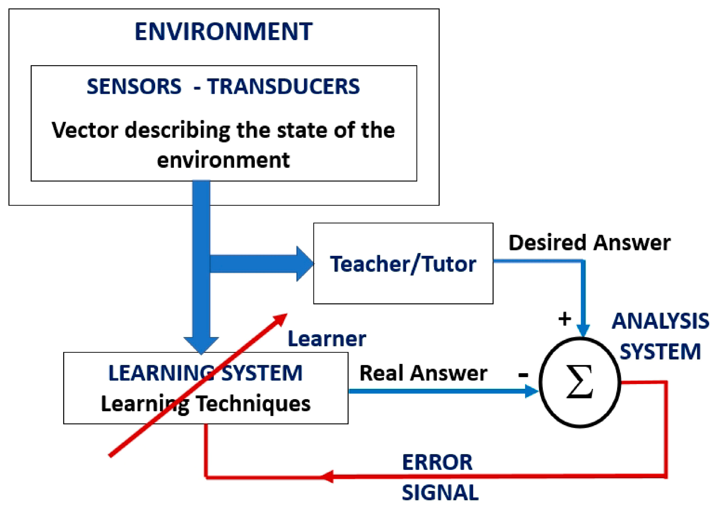
2. Fundamentals of Learning from Demonstration (LfD)

In systems dedicated to the control of automation, trajectories, and robot movement, highly complex algorithms are used. The programming of the computational modules of these machines uses dedicated and structured algorithms so that the machines can perform tasks that are related to the movement and transport of objects with precision [29]. However, with each change in the machine trajectory or changes in transported products, there is a need for the intervention of programming specialists to adapt the system to these new tasks [29,30,31]. In industrial production systems where robots act in complex actions, reprogramming to adapt the machines can make production unfeasible. Thus, learning from demonstration (LfD) would be a method that would provide greater speed in modifying machine movement strategies, where, in this case, the knowledge transfer process would use the concepts of human learning. Thus, flexibility in machine programming would have to be adapted with algorithms capable of transferring skills through direct intervention, observation, goal emulation, imitation, and other social interactions [32,33,34,35].

2.1. Machine Learning

Machine learning is used to teach machines how to handle the data more efficiently. As can be seen in [36], machine learning methods can be classified into four types: 1. supervised learning; 2. unsupervised learning; 3. semi-supervised learning; and 4. reinforced learning.

2.1.1. Supervised Learning

Supervised learning, which is considered to be LfD with the support of a system composed of artificial neural networks, can be classified into three stages: demonstration, learning, and imitation. These steps will be described below [36,37].
(1) Demonstration—This is where the Tutor performs the desired activities for the robot to learn. In a practical process, it is considered that the Learner and the Tutor are exposed to a training vector. The Tutor, based on his knowledge of the environment, has the ability to provide a response to the artificial neural network, which represents the optimal action to be performed by the learner according to the training vector;
(2) Learning—In this step supervised learning takes place. This is where the parameters of the artificial neural network are adjusted based on the training vector and on the error signal, which is defined by the difference between the desired response and the real response of the network. In this step, the artificial neural network simulates the Tutor, transferring the knowledge of the environment to the Learner. In general, the optimization of the emulation is verified through statistical calculation to confirm that the knowledge of the environment is transferred to the learner in a complete way;
(3) Imitation—At this stage, the learning condition is complete, and the artificial neural network has finished its training process transferring the knowledge obtained from the Tutor to the Learner. Therefore, the Tutor is no longer needed, and the Learner, after receiving the information from the artificial neural network, is able to recognize and deal with the environment without the need for external help.
Figure 1 shows a block diagram on the main steps of supervised learning [37,38].
The “Learning Techniques” block in Figure 1 is related to machine learning techniques, therefore it is where we will use an LfD method that is applied with Paraconsistent Logic algorithms.

2.1.2. Demonstration Step Approaches

In general, three forms of approaches are used for the demonstration stage.
The first is known as kinesthetic, which is where the Tutor physically demonstrates the moving actions to the robot or machine through the desired movements or trajectories. In this case, the robot states during the interaction are registered through its integrated sensors (e.g., joint angles and torques), resulting in training information data for the machine learning model [37,38].
The second form of demonstration is called teleoperation. In this category, there is no requirement for the Tutor to be in direct contact with the Learner (which, in this case, is the robot). For this demonstration technique, an external input is required to drive the machine or robot; this can be via a joystick, a graphical interface, or other means. This mode allows LfD techniques to be applied in remote environments, and information about the robot’s states during movement is registered through its integrated sensors.
The third demonstration approach is the Passive Observations or Motion-Sensor Demonstration method. In this approach, the Tutor performs the task using their own body, which can sometimes be implemented with additional sensors to facilitate tracking [36,37,38]. Information data about the machine’s states and trajectories are registered by means of tracking sensors.

2.2. Data Modeling for Feature Extraction

The demonstration learning technique brings numerous challenges to its application; among these main problems is the data modeling mode for the extraction of features. This phase encompasses two main issues that need to be discussed. The first is how to interpret and understand the data arising from observed behaviors—in other words, the problem is how to recognize human behavior (Tutor) from information data. To achieve the robot (Learner) learning from the demonstration, it is necessary to address the matching problem, which means finding ways to map links and joints from a human (Tutor) to a robot (Learner) [39,40]. The second is how to integrate the systems of perception and movement control to reconstruct what is observed. Therefore, methods must be found to structure the motor control system for general movement and imitation learning capabilities. Faced with these challenges, current approaches are divided into two trends: the first uses trajectory coding, which is a low-level representation of skill, in the form of a non-linear mapping between sensory and motor information; the second trend has used symbolic coding, which is a high-level representation of a skill that breaks down a skill into a sequence of action perception units [41,42].

2.3. Modeling

In this learning from demonstration system, generalization is important since it should be possible to model a demonstrated movement with different goal positions. Another important feature is that a learning from demonstration model must also be robust against disturbances, as exactly repeating an observed movement is not realistic in a dynamic environment in which obstacles can suddenly appear. Due to this and other factors, the data collected in the demonstration approaches need to be mapped through a mathematical model to compose the algorithmic models that will enable imitation acts. Therefore, systems operating in LfD require a learning policy to extract and generalize the main features of assembly movements [42]. In [39,40], Hidden Markov Models (HMMs) were used to code and generalize the demonstration examples. In the normal Markov model, the state is directly visible to the observer; therefore, the transformation probabilities between states are the whole parameters. While the states are not visible in the Hidden Markov Model, some variables that are influenced by the states are visible. Every state has a probability distribution on a token of possible output; therefore, the sequence of the output token reveals the information of the state’s sequence. The Hidden Markov Model (HMM) is a robust probabilistic method that is used to encapsulate human movement; it contains both spatial and temporal variables that are used for numerous demonstrations [40].
Another modeling method that has shown good results was included in [41,42,43], where the authors used dynamic motion primitives (DMPs), which represent a fundamentally different approach to representing motion, one that based on nonlinear dynamical systems.
Dynamical systems with global asymptotic stability define a function that represents a global navigation map where all space trajectories converge to the target [41]. Therefore, when used to code trajectories, this characteristic of dynamic systems ensures that every trajectory, within the regions of asymptotic stability, collaborates with the correct direction to reach the target from the robot’s current position. If the robot or machine suffers any spatial disturbance that is caused by an actuation or sensing error that introduces small deviations in the execution of its trajectory, it will still be able to reach the target if the deviations do not remove it from the stability region [43]. Modeling with this technique also allows the system to be able to deal with the temporal disturbances that are caused by communication delays and the dynamics of low-level controllers. An alternative for the system to be robust to these temporal disturbances is that it be autonomous, i.e., independent of time [39,42,43].
As seen in [41,42,43], DMP is robust to spatial perturbations and is suitable for the purpose of following a specific motion path, so it is one of the modeling techniques that has responded robustly to perturbations in LfD architectures.
In this article, we aim to present an algorithm based on Paraconsistent Logic, the Learning Paraconsistent Artificial Neural Cell- lPANCell [44] algorithm, which holds the characteristics of modeling by DMP, which is applied in the process of learning the range movements of robotic machines from a set of demonstrations [41,45]. Each demonstration is a trajectory in the linear Cartesian robotic machine’s workspace, which has the task of moving rectangular metal workpieces in an industrial production process [46].
The information data corresponding to the trajectories are obtained through the robotic machine being controlled by a joystick operated by a human, where the positions are collected and transformed into learning patterns. After learning, the robotic machine will be able to reproduce, without human interference, trajectories that are similar to the demonstrations. In the imitation stage, the robotic machine, which has learned through the LfD process, should show robustness to the temporal disturbances caused by communication delays, as well as to the spatial disturbances caused by some actuation or sensing error. The trajectories are similar to the demonstrations that are executed by the robot, even when starting the movement from points that are different from the demonstrations, and even with the change in the target position occurring during the execution of the procedure [46,47].

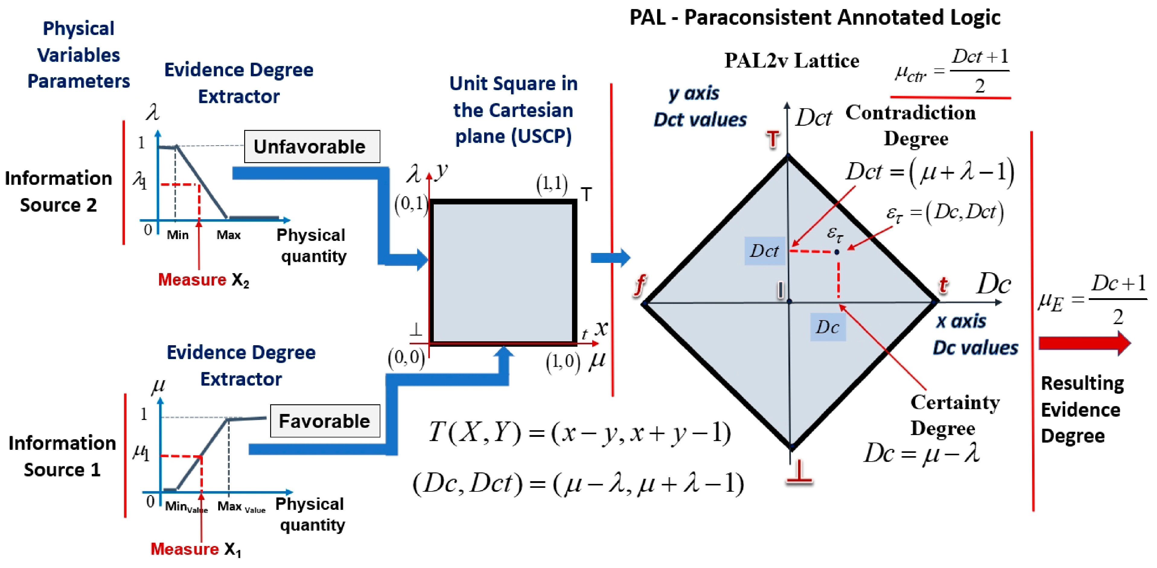
3. Paraconsistent Logic (PL)

Paraconsistent Logic (PL) belongs to a non-classical logic category, and its main feature is the revocation of the principle of non-contradiction [48]. In [49], PL was described with its equations and all its predicates being formalized; it was studied in completeness, and was demonstrated to be an example of non-classical, propositional, and evidential-based logic.
In [6], the authors presented an extension of PL called Paraconsistent Annotated Logic (PAL), which is associated with a four lattice system, wherein its vertices are considered representations of the following logical states: t = true, f = false, T = inconsistent, and ⊥ = paracomplete. In this representation, the logical states refer to a proposition P that is under analysis. In this mode of interpretation, an annotation composed of two degrees of evidence (µ, λ) assigns a logical connotation to a proposition P, such that µ represents the degree of evidence in favor of proposition P, and λ represents the degree of evidence against proposition P.
The degrees of evidence are extracted from different information sources and have their values normalized, thus belonging to a set of real numbers. Therefore, µ, λ ⊂ [0, 1] ∈ R .
Thus, the annotation (µ, λ), in the condition of maximum values, represents the extreme logical states of the lattice vertices, which are according to the values of µ and λ below:
(1,0)—favorable evidence degree to proposition P maximum and unfavorable evidence degree to proposition P minimum resulting in a logical state t = true;
(0,1)—favorable evidence degree to proposition P minimum and unfavorable evidence degree to proposition P maximum resulting in a logical state f = false;
(1,1)—favorable evidence degree to proposition to P maximum and unfavorable evidence degree to proposition P maximum resulting in a logical state Τ = inconsistent;
(0,0)—favorable evidence degree to proposition P minimum and unfavorable evidence degree to proposition P minimum resulting in a logical state ⊥= paracomplete.
As the values of µ and λ can vary between 0 and 1 and belong to the set R , then infinite logical states, with their variations, can be considered internally in the lattice.
Algebraic interpretations can relate to the degrees of evidence used in the logical states of the PAL2v lattice.
Through the representations of values, with favorable evidence degree μ on the x axis and unfavorable evidence degree of λ on the y axis in a Unit Square in the Cartesian Plane (USCP), it is possible to obtain a transformation (T), shown in Equation (3), that represents these values in a lattice that is associated with PAL [6,49,50].
T ( X , Y ) = ( x y , x + y 1 )
Relating the lattice associated with PAL with components of the transformation T(X, Y) from Equation (3), we have
x = μ → degree of favorable evidence, with 0 ≤ μ ≤ 1
  y = λ → degree of unfavorable evidence, with 0 ≤ λ ≤ 1
The first term obtained in the ordered pair of the Equation (3) is X = x y = μ λ →, which is called the degree of certainty (Dc), and the second term is Y = x + y 1 = μ + λ 1 →, which is called the degree of contradiction (Dct). Therefore, the degree of certainty is obtained by Equation (4).
D c = μ λ
and the degree of contradiction is obtained by Equation (5).
D c t = μ + λ 1
The resulting evidence degree (μE) is calculated by the degree of certainty normalization, as is the case in Equation (6):
μ E = D c + 1 2
Additionally, the normalized contradiction degree (µctr) is calculated by μ c t r = D c t + 1 2 or by Equation (7):
μ c t r = μ + λ 2
With these PAL2v-equations, we can build algorithms for the analysis and comparison of signals through paraconsistent logic [4,6,49].
Based on Equations (5) and (6), a pair of values (Dc, Dct) is formed that provides a single point located within the lattice associated with PAL, thus defining a paraconsistent logical state [50,51,52].
Figure 2 shows a Unit Square in the Cartesian plane (USCP) with the evidence degrees µ and λ exposed on the x e, and y axes, and with the PAL lattice with a paraconsistent logic state composed by the pair (Dc, Dct).
The degrees of evidence originate from different sources, vary in the range between 0 and 1, and belong to a set of real numbers. Thus, this annotation of two values (µ, λ) can generate infinite points and can consequently generate infinite logical states (Dc, Dct) in the associated PAL lattice [6,50,52].

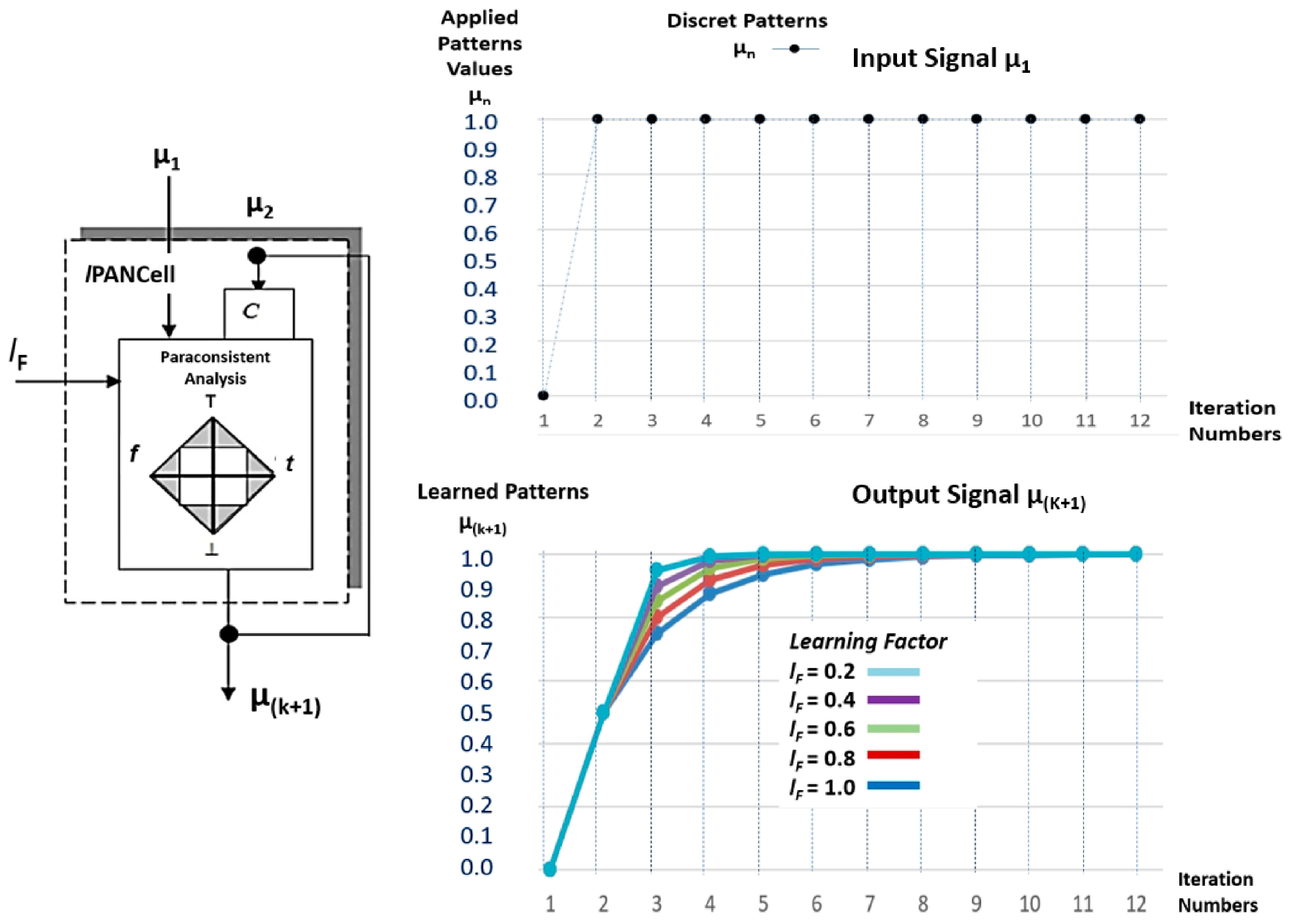
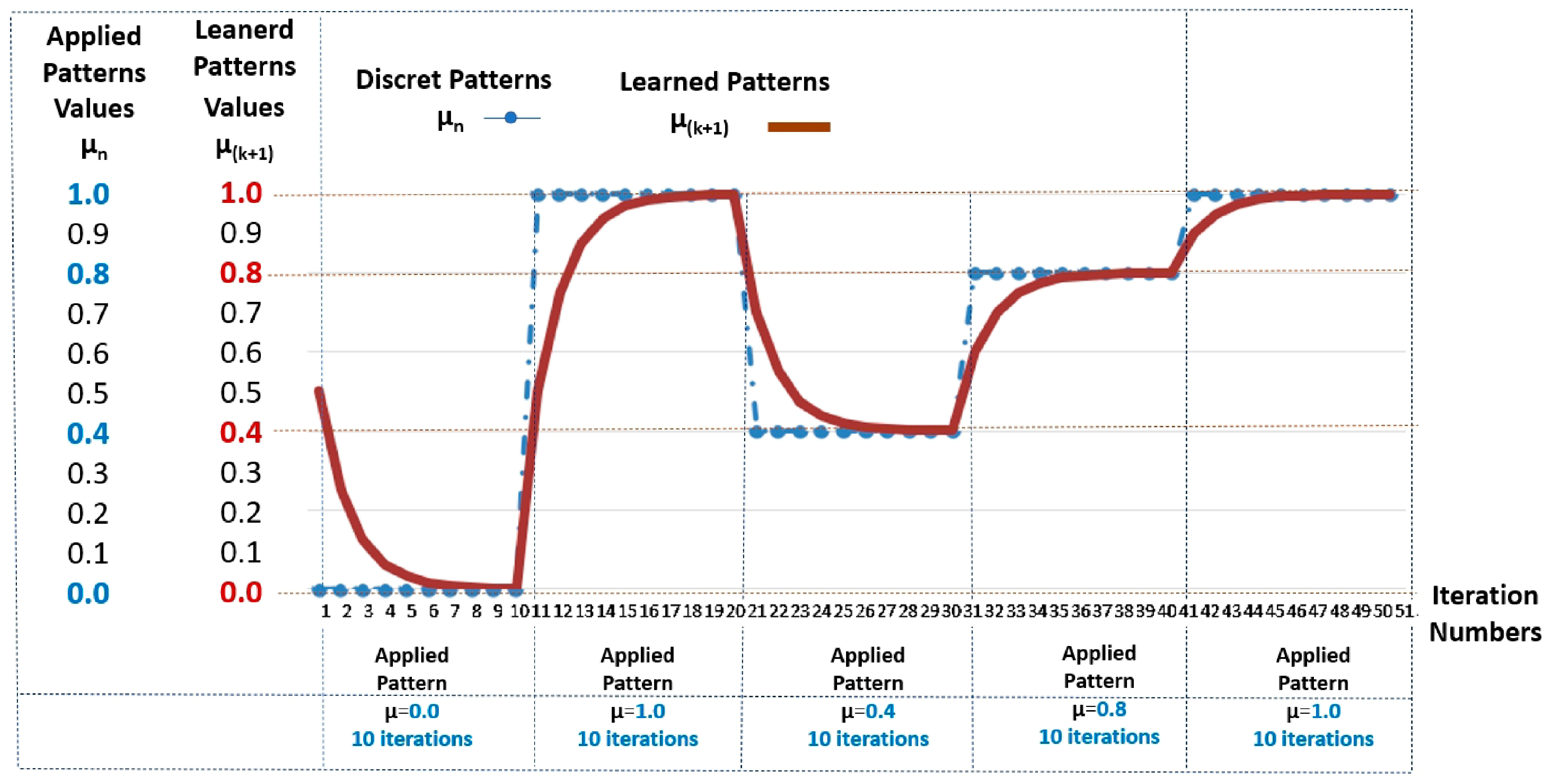
3.1. Paraconsistent Artificial Neural Cell of Learning (lPANCell)

As the Paraconsistent Logic Annotated with Annotation of Two Values (PAL2v) model has the ability to handle information that is considered incomplete and contradictory, then some algorithmic structures built with its equations may indicate similarities with the biological mental process.
In [6], a family of PANCells—Paraconsistent Artificial Neural Cells—was presented to compose computational structures that are capable of showing results similar to some behaviors of the human brain. Through an algorithm configured with Equation (4), a basic Paraconsistent Artificial Cell (PACellb) was considered, which—from the signals received at the input and from external adjustment factors—makes the decision, based on levels of resulting values in your output. Using PACellb as a basis, Paraconsistent Artificial Neural Cells were built, which were of different types and with specific purposes [4,51,53].
In this work, we use the Paraconsistent Artificial Neural Cell of Learning (lPANCell) model, which can be trained to learn patterns that are between the real values of 0 and 1. Initially, it was considered that the pattern in a lPANCell is defined as a binary digit, in which 1 is equivalent to the “true” logic state and the value 0 means a “false” logic state. From Equation (4), it is possible to obtain a single recurrence equation so that the degree of unfavorable evidence λ is obtained from the complement of the degree resulting from the output [6,49,50,51,52,53]. Considering that μ 1 is the value of the learning pattern in the current state, and μ E ( k + 1 ) is the value of the later state—that is, the learned value—then the lPANCell equation to obtain the Resultant Evidence Degree μ E is represented by Equation (8):
μ E ( k + 1 ) = μ 1 ( μ E ( k ) c ) l F + 1 2
with μ E ( k ) c = 1 μ E ( k ) and k as the number of iterations, and l F = Learning Factor.
The lPANCell equation to obtain the normalized contradiction degree μ c t r is represented by Equation (9) [6,12]:
μ c t r ( k + 1 ) = μ 1 + ( μ E ( k ) c ) l F 2
The lPANCell is considered completely trained when μ E ( k + 1 ) = 1 and μ c t r ( k + 1 ) = 0 .
If the pattern applied to the cell input is unitary ( μ 1 = 1 ), then the output will converge to μ E ( k + 1 ) = 1 with a monotonic variation, whose number of iterations (n) for the output to reach this maximum value will depend on the lF value [4,7,13].
With the values obtained in Equations (8) and (9) we can represent the learning state of lPANCell by Equation (10):
( μ E ( k + 1 ) , μ c t r ( k + 1 ) )
Therefore, the simplified algorithm with a learning factor set in l F = 1 , for the learning of any value between 0 and 1, is shown in the Algorithm 1 below [6,7,13].
Algorithm 1: Paraconsistent Artificial Neural Cell of Learning—lPANCell
1. Initial Condition
μ 1 = 1 / 2 and μ 2 k = μ 2 = 1 / 2
2. Enter the value of the Learning Factor
( l F = 1 )         */Learning Factor */
3. Transform the Degree of Evidence 2 into Unfavorable Degree of Evidence
λ 2 k = 1 μ 2       */Unfavorable Degree of Evidence */
4. Enter the Pattern value (Degree of Evidence of input 1)
μ 1 = 1             */Degree of Evidence */
5. Compute the Resultant Evidence Degree (Equation (6)).
            μ E ( k + 1 ) = { μ 1 ( λ 2 ) l F } + 1 2
6. Compute the Normalized Contradiction Degree (Equation (7)).
            μ c t r ( k + 1 ) = { μ 1 + ( λ 2 ) l F } 2
7. Present the current state of learning (Equation (10)).
            ( μ E ( k + 1 ) , μ c t r ( k + 1 ) )
8. Consider the condition
     If μ E ( k + 1 ) 1 Do μ E ( k + 1 ) = μ 2 and return to step 3
9. Stop
Figure 3 shows the symbol of the lPANCell, as well as the graphs with the curves corresponding to the outputs (μ(k+1)) that were obtained with 12 iterations of the pattern μ1 = 1, with learning factor values adjusted to lF = 1, lF = 0.8, lF = 0.6, lF = 0.4, and lF = 0.2.
It was verified that after repeatedly receiving its input, the value of the pattern μ1 resulted in an ascending monotonic curve appearing, which demonstrates the cell’s learning after the convergence in output μ(k+1) = 1.0.
When the value of the learning factor is set to lF = 1, the lPANCell will need more steps (iterations) to complete a training; in this case, it is characterized as a natural learning capacity [6].
Convergence for patterns of values between 0 and 1 only happens for the learning factor set in lF = 1. With the learning factor set to lF = 1, and by applying its input μ1 to the value of 0 repeatedly, a descending monotonic curve appears that demonstrates the unlearning of the cell when the convergence reaches in output μ(k+1) = 0.0 [6].
Table 2 shows the values obtained in the simulation of an lPANCell with the learning factor set at lF = 1 in the sequential application of five patterns with different values.
The test was conducted with 10 iterations each.
Figure 4 shows the values obtained in the form of graphs [4,7,13].
When the lF value is other than 1, the output will not converge to the input pattern value if the u1 pattern is different from 1. In this case, adaptations must be made to the input values with a compensation in the output values [13].

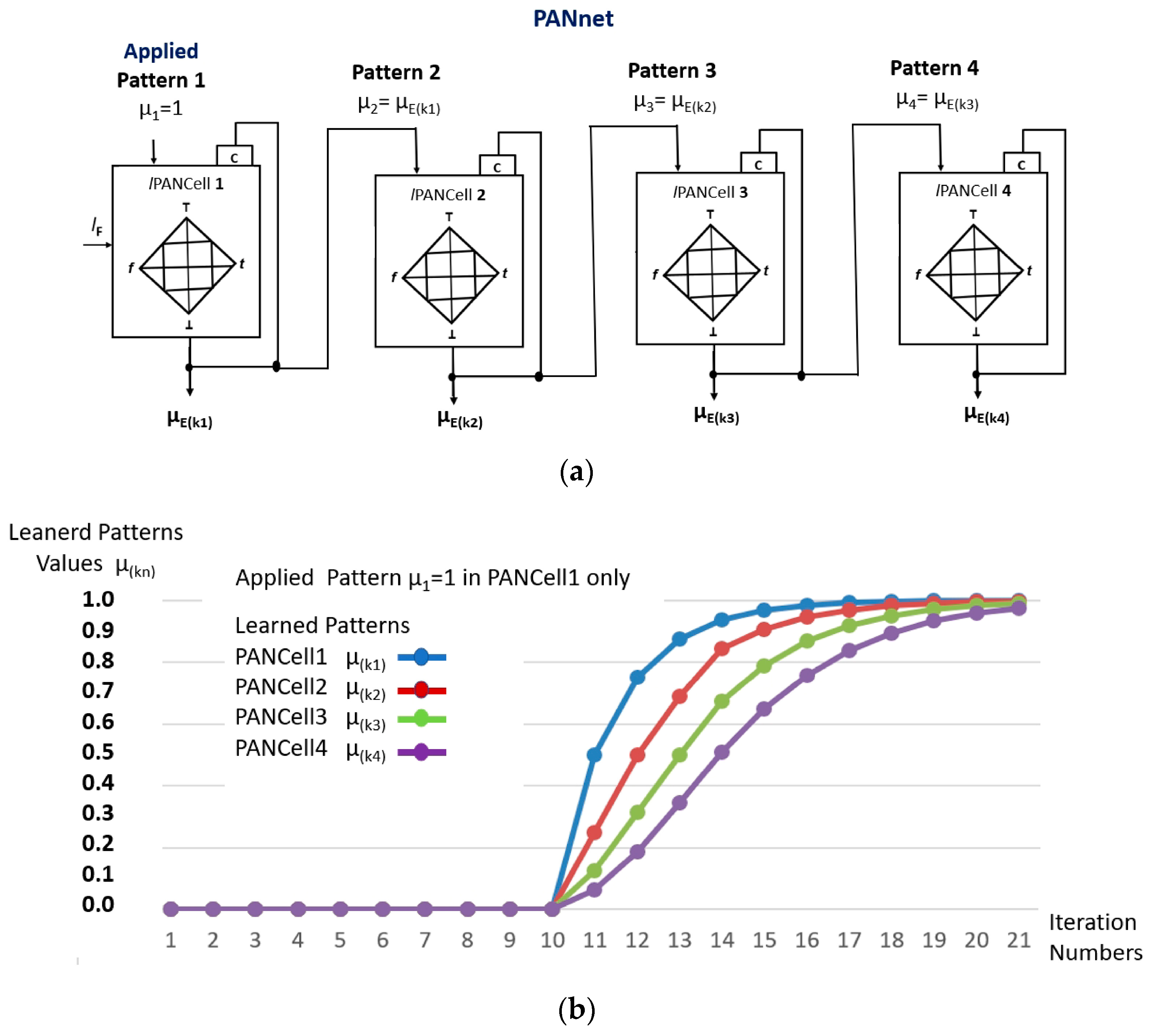
3.2. lPANnet—Paraconsistent Artificial Neural Network

The lPANCell model can be interconnected and can form different configurations of a paraconsistent artificial neural network for the purposes of an analysis of information signals that are formatted into degrees of evidence.
As seen in [13], it is possible to build a configuration of lPANCells that are interconnected in a cascade, and where the output of the first lPANCell (μ(kn1)) is the same pattern applied to the second, etc. In this case, the pattern applied to the first lPANCell will have a response that is twice as fast as the second lPANCell, etc.
Figure 5a shows a structure of an lPANnet composed of four lPANCells that were configured in a cascade. Simulations were carried out where, initially, applications of Pattern µ1 = 0 were made in the first lPANCell; these consisted of an unlearning process and, soon after, pattern µ1 = 1 was applied for 12 iterations.
The values shown in Table 3 refer to the results obtained from the four outputs of the lPANCell that make up the configuration [6,7,13].
Figure 5b shows the results, in graph form, that were obtained in the learning process of the lPANnet configuration in 12 iterations.

4. Materials and Methods

In this work, the lPANCell algorithm was implemented, with non-classical logic characteristics, in a Programmable Controller (PC) in the form of a functional block (lPANC_BLK) to be used in the control device of a linear Cartesian robot (gantry robot). The programming of the function block followed IEC 61131-3 standards [54], which aim to standardize programming languages and its structure in programmable controllers.

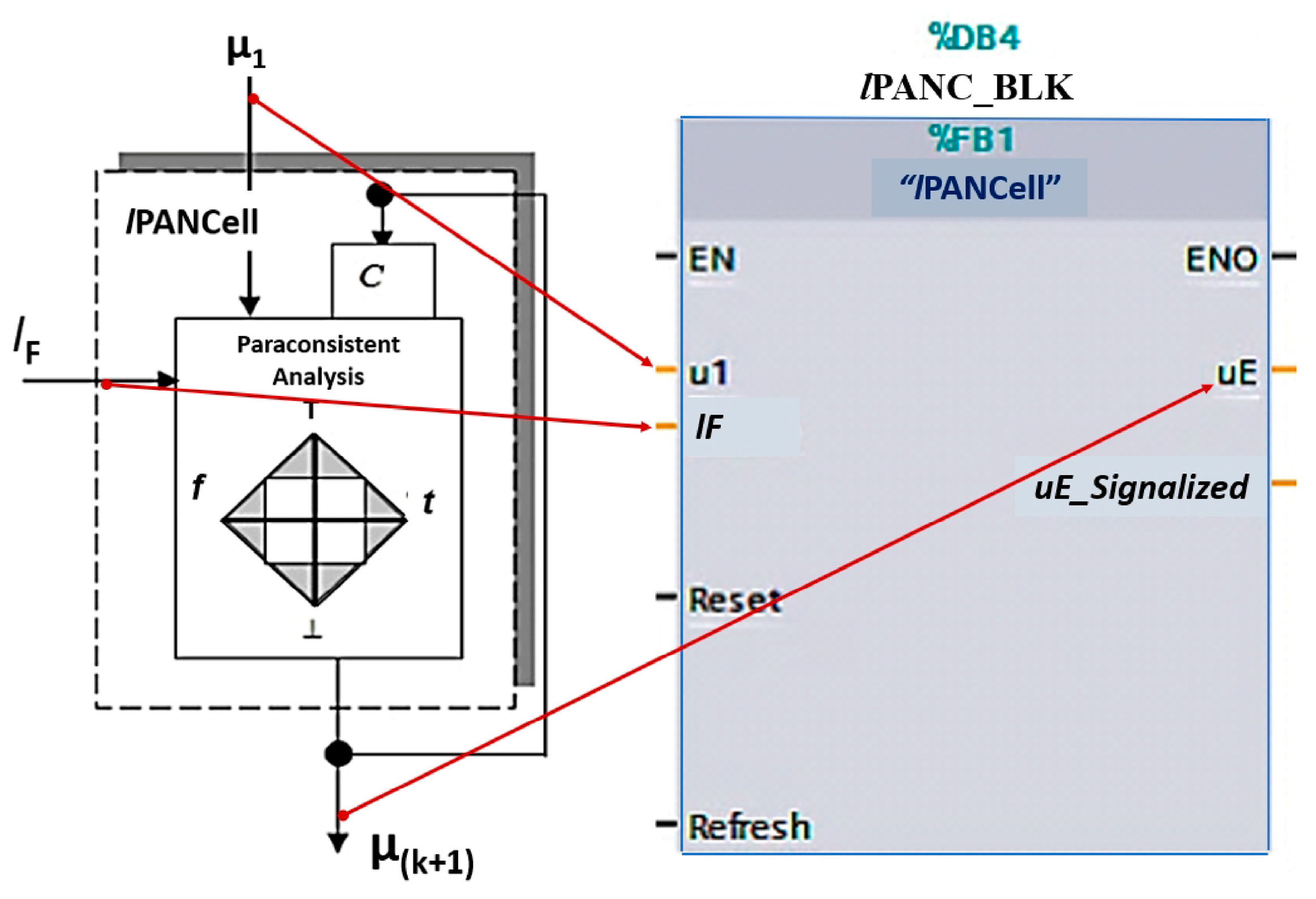
4.1. Functional Block (lPANC_BLK)

In the construction of the function block (lPANC_BLK) that was based on the learning Paraconsistent Artificial Neural Cell algorithm (lPANCell), the Programmable Controller (PC) from the manufacturer SIEMENS model S7-1500 was used. The program was developed using SIEMENS (TIA Portal)-Totally Integrated Automation Portal software [55].
The internal programming of the function block (lPANC_BLK) was carried out based on the lPANCell algorithm, in which the Ladder language was chosen due to its wide use by professionals in the industrial automation area.
Figure 6 shows the lPANC_BLK symbol that was built based on the IEC 61131-3 standard [54] and the corresponding nomenclatures between the function block and the lPANCell symbol.
To the left of the lPANC_BLK block are the inputs: EN (enable), input pattern u1, learning factor lF, reset signal, and refresh signal. The output variables, which are located to the right of the block, are ENO (enable output), degree of the evidence of the output (uE), and signaling signal (uE_Signaled). To provide a better analysis of the behavior of the lPANC_BLK block, the values of lF, u1, and uE were normalized in the range between 0 and 100. Therefore, these three values were proportional to the normalized values of lPANCell, which is between 0 and 1.
The function of the input and output variables of lPANC_BLK are described below:
(a)
EN: Enable the block when its logic level is 1;
(b)
u1: Input pattern to be learned by lPANC_BLK in the range 0 to 100;
(c)
lF: Learning factor that corresponds to an adjustment of how quickly the cell will learn the input pattern—adjusted in the range of 0 to 100;
(d)
Reset: Restart the block, assigning the value 50 to the output μE.
The lPANC_BLK block, when receiving a pulse on the reset input, generates at its output uE the value 50, which corresponds to the value 0.5 in the lPANCell algorithm. The cell is then ready to start learning (or unlearning).
(e)
Refresh: Updates the input pattern after receiving a pulse at logic level 1;
(f)
ENO: Provides logic level 1 when block is active;
(g)
uE: Evidence degree, which corresponds to the block output in the range of 0 to 100;
(h)
uE_Signaled: Signaling with a value of 100 when the block ends learning (or unlearning).

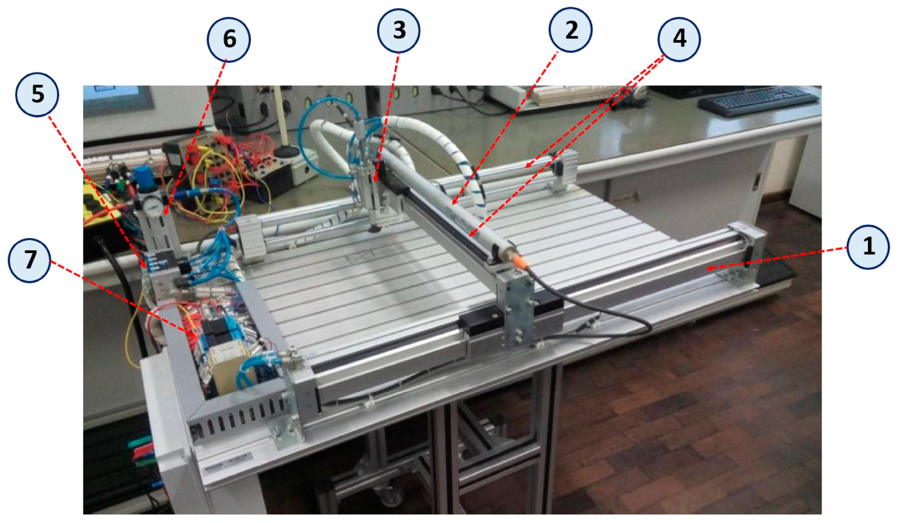
4.2. Linear Cartesian Robot and Pneumatic Machine Tool

The lPANC_BLK block was installed in the Programmable Controller (PC) of a linear Cartesian robot (gantry robot), which operates in a pneumatic machine tool whose task is to move metal workpieces in an industrial system [46,47,55].
The structure of the linear Cartesian Robot (gantry robot) composing the pneumatic machine tool is shown in Figure 7.
We can see in Figure 7 that the pneumatic machine tool consists of a double-acting rodless cylinder structure (1), whereby the gantry mounts a sliding crossbar to trigger the movements that are performed on the X axis. In addition, a double-acting rodless cylinder is fixed to the previous cylinder (2), which has the function of driving the support assembly that moves on the Y axis, which is where a gripping device is coupled with magnetic workpieces that are driven by a hollow through-rod cylinder with a suction cup (3). This suction cup’s function is to move two linear transducers X and Y (4) along the Z axis, as well as to operate an electropneumatic valve block (5), an air-compressed unit (6), and a set of terminals (7) for the electrical control interface.

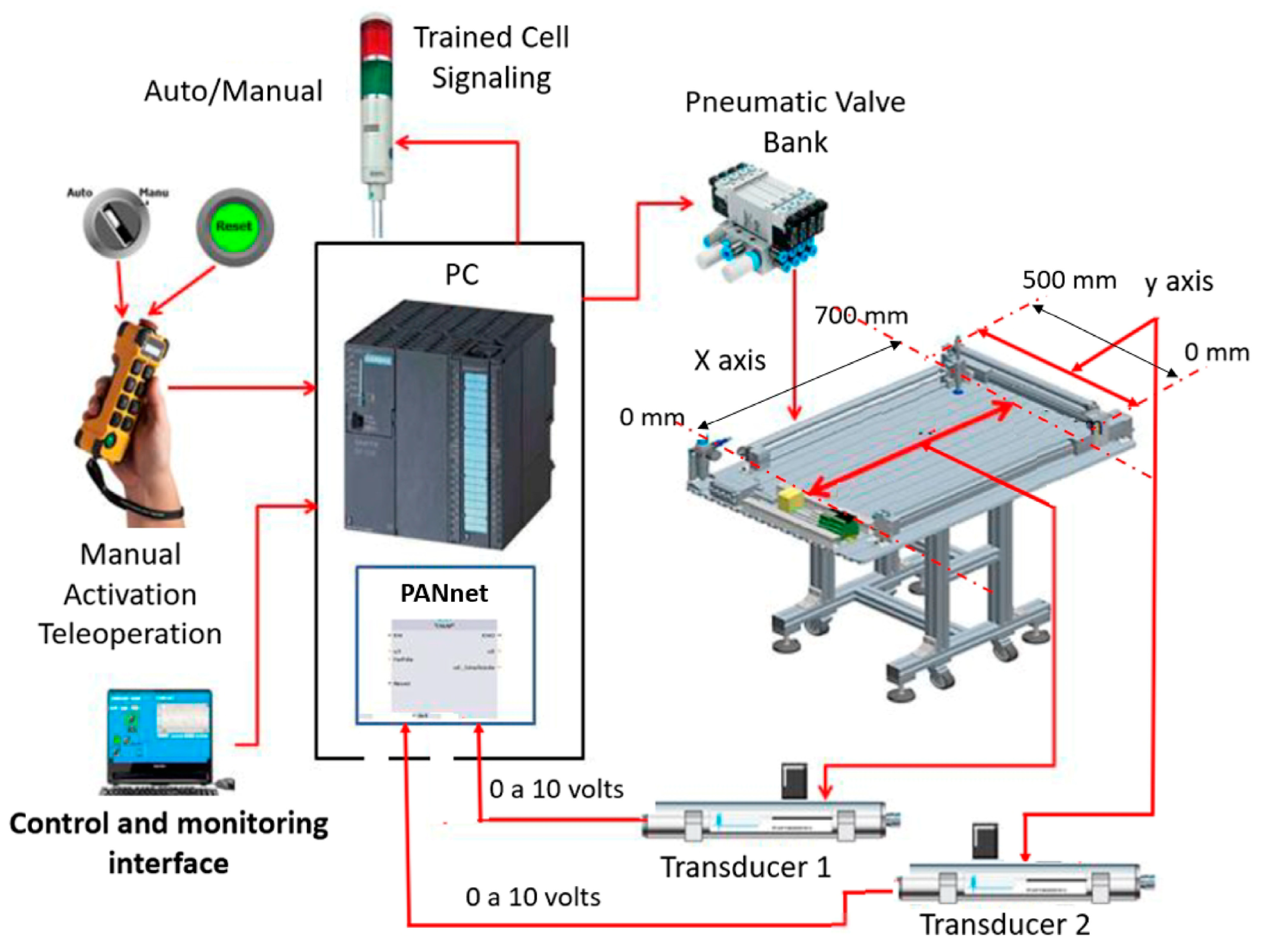
4.3. Practical Application—Forms of Activation and Control

In practice, the lPANnet computational structure (composed of lPANC_BLK functional blocks) acts in an LfD process to teach trajectories (on the x and y axes) to a linear Cartesian robot (gantry robot) to be able to work on moving rectangular metallic workpieces on the table of an electropneumatic machine tool.
As shown in Figure 8, the machine contains a triangular table with dimensions 670 × 890 mm. This is where the metallic workpieces are moved through the action of the linear Cartesian robot (gantry robot). The dimensions that are useful for delimiting the trajectories x and y through which the linear Cartesian robot (gantry robot) works are 500 × 700 mm. Therefore, the drive assembly of the linear Cartesian robot, which is composed of the cylinder-driven sliding crossbar, can move in a 700 mm extension, which is the table length, on the X-axis. In addition, the support carrying the magnetic gripper is driven by another cylinder and can move 500 mm on the Y-axis. The magnetic workpiece gripper device captures one metallic workpiece at a time and is capable of moving around 20 mm on the Z axis.
For the LfD process, the pneumatic machine tool has a manual push button (joystick), a programmable controller (PC), two displacement transducers, a flag device (5), and other support devices, as shown in Figure 8. The electronic system composed of the PC and electronic devices controls the movement of the workpiece magnetic gripping device from a determined point as the origin (X0, Y0) to the place of deposition of the workpieces, which is stipulated as the objective point of the trajectory (X(Target), Y(Target)). Two transducers measure the distances traveled in moving the slider bar (X-axis transducer) and moving the workpiece magnetic gripping device support (Y-axis transducer).
The pushbutton (joystick) has movements on the XYZ axes, and its activation can occur manually through a remote control. The program inserted in the Programmable Controller (PC) was made in such a way that when putting the system into manual operation the lPANC_BLK Block will enter the learning mode.

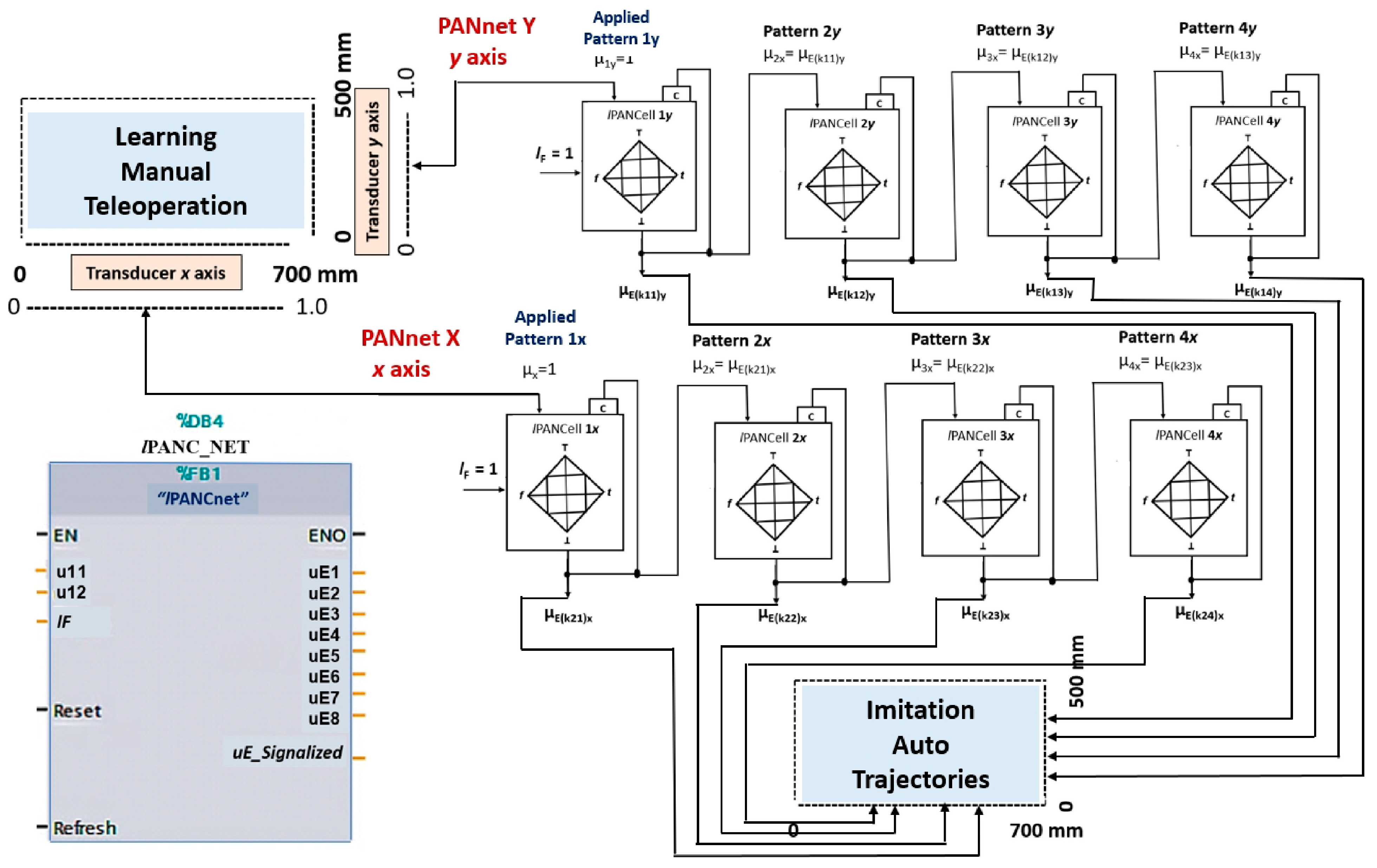
4.4. Paraconsistent Artificial Neural Network (lPANnet) Configured with lPANC_BLK Blocks

In the Programmable Controller, a program was installed that forms a structure composed of a set of 8 lPANC_BLK blocks forming a Paraconsistent Artificial Neural Network (lPANnet) that will operate in the LfD process.
Figure 9 shows the configuration of the lPANCells that were formed through the lPANC_BLK blocks.
Each group of 4 lPANC_BLK blocks interconnected in a cascade will be trained separately.
The first group (lPANnet Y) receives the pattern from the Y transducer and learns the trajectory demonstrated by teleoperation on the y-axis.
The second group (lPANnet X) receives the pattern from the X transducer and learns the trajectory demonstrated by teleoperation on the x-axis.
The imitation step can be conducted by choosing one of the 16 possible trajectories in the x and y axes, established by the transition states (Xn, Yn) that are represented by the output values of the second group (lPANnet X) and first group (lPANnet Y), respectively.
The lF values of each lPANCell and the composition of the computational structure that make up the lPANnet allow for obtaining trajectory adjustments, as well as obtaining the velocities linked to the transition period of the states, thus resulting in linear or non-linear trajectories.

4.4.1. Planning

In this work, due to the characteristics of the machine tool, the trajectories were planned as shown below.
X-axis trajectory: start X0 = 0 mm    finish X(Target) = 700 mm
Y-axis trajectory: start Y0 = 0 mm    finish Y(Target) = 500 mm
If the learning factor is set to lF = 1, then 12 iterations are required for a complete learning of µ(k+1) = 1.
The advance corresponds to the resulting degrees of evidence and, in this way, the trajectory of the movement is fulfilled through the variations in the transition states. The lF adjustment values will influence the trajectory behavior where advances will be greater at the beginning and will then decrease at the end of learning.
The training process was carried out with the button selected in manual mode (teleoperation).
Although the learning was estimated to be completed after 10 iterations, the occurrence of interferences in learning can lead to more iterations being necessary for the output of lPANC_BLK to better indicate the completed learning value. Thus, the system was adjusted so that, after the necessary iterations, the lPANC_BLK indicated the maximum value of µ(k+1) = µ1 with the “Trained Cell” signal. After this signal, the linear Cartesian robot, which drives the machine tool, was available for the “Imitation” step, where the system works without operator intervention.
The “Demonstration Step” was performed in two stages:
  • Learning from demonstration on the x-axis determining the trajectory gx = X(Target)X0;
  • Learning from demonstration on the y-axis determining the trajectory gy = Y(Target)Y0.
This makes the linear Cartesian robot activate the support assembly where the magnetic workpiece gripper device is attached, which fulfills the moving of the workpieces in the trajectory that was established by the learning of advances in both axes.

4.4.2. Learning Stage (Teleoperation)

(a)
First gx trajectory—Advance of the pneumatic cylinder on the x axis
In possession of the button (joystick), the Tutor activates the machine tool (Learner) n times, causing the support with the magnetic grabber to capture the metallic workpiece at point X0 and to move it to the indicated point X(Target). With the movement of the magnetic grabber, the displacement transducer on the x axis brings the information of the cylinder advance in the form of an evidence degree (a value between 0 and 1), which is applied in the cells that are implemented in the lPANC_BLK x blocks.
In this step, the first lPANCell cell programmed in the lPANC_BLK x1 block learns the pattern corresponding to the advance distance of the trajectory gx, so its output after each iteration will present a value corresponding to the advance distance gx = X(Target)X0. In complete learning, the value at the outputs of all 4 lPANCells will be maximum µ(k+n)xn = 1 that corresponds to the maximum permissible advance on the machine tool table (700 mm).
(b)
Second gy trajectory—Advance of the pneumatic cylinder on the y axis
The Tutor activates the machine tool (Learner) n times causing the magnetic gripper to capture the metallic workpiece at point Y0 and move it to the indicated point Y(Target). With the movement of the magnetic grabber, the displacement transducer on the y axis brings the information of the cylinder advance in the form of evidence degree (value between 0 and 1) that is applied in the cells implemented in the lPANC_BLK y blocks. In complete learning, the value at the outputs of all 4 lPANCells will be a maximum µ(k+n)yn = 1, which corresponds to the maximum permissible advance on the machine tool table (500 mm).
Completing the procedures to lPANnet, which comprises the 4 lPANC_BLK x blocks and the 4 PANC_BLK y blocks, results in the 16 possible coordinates of the trajectories that were learned via LfD to be stored in robot’s outputs. The signal that the learning has been completed (uE_Signaled) is generated by the lPANC_BLK network and makes it such that the procedures for moving the metallic workpieces are activated.

4.4.3. Imitation Step

After the information in the outputs (μ(k+1)) of the lPANC_BLK function blocks indicate that the learning by demonstration of the gx and gy trajectories has been completed, the machine tool control system is activated and is responsible for activating the mobile device with a magnetic grabber.
With the 4 lPANC_BLK x blocks that store the transition states in the x axis and the 4 lPANC_BLK y blocks that store transition states in the y axis, it is possible to configure a linear Cartesian robot actuation with 16 different trajectories.

5. Results and Discussion

In this work, the lPANCells were arranged in a cascade forming two groups that compose the Paraconsistent Artificial Neural Network (lPANnet). This type of configuration allows 16 different trajectories to be obtained, where the transition states are represented by the values (Xn,Yn) of the outputs of the lPANCells that were programmed in the form of the functional lPANC_BLK x and lPANC_BLK y blocks.
For this study, the 16 possible trajectories were classified into four types considering their linearity:
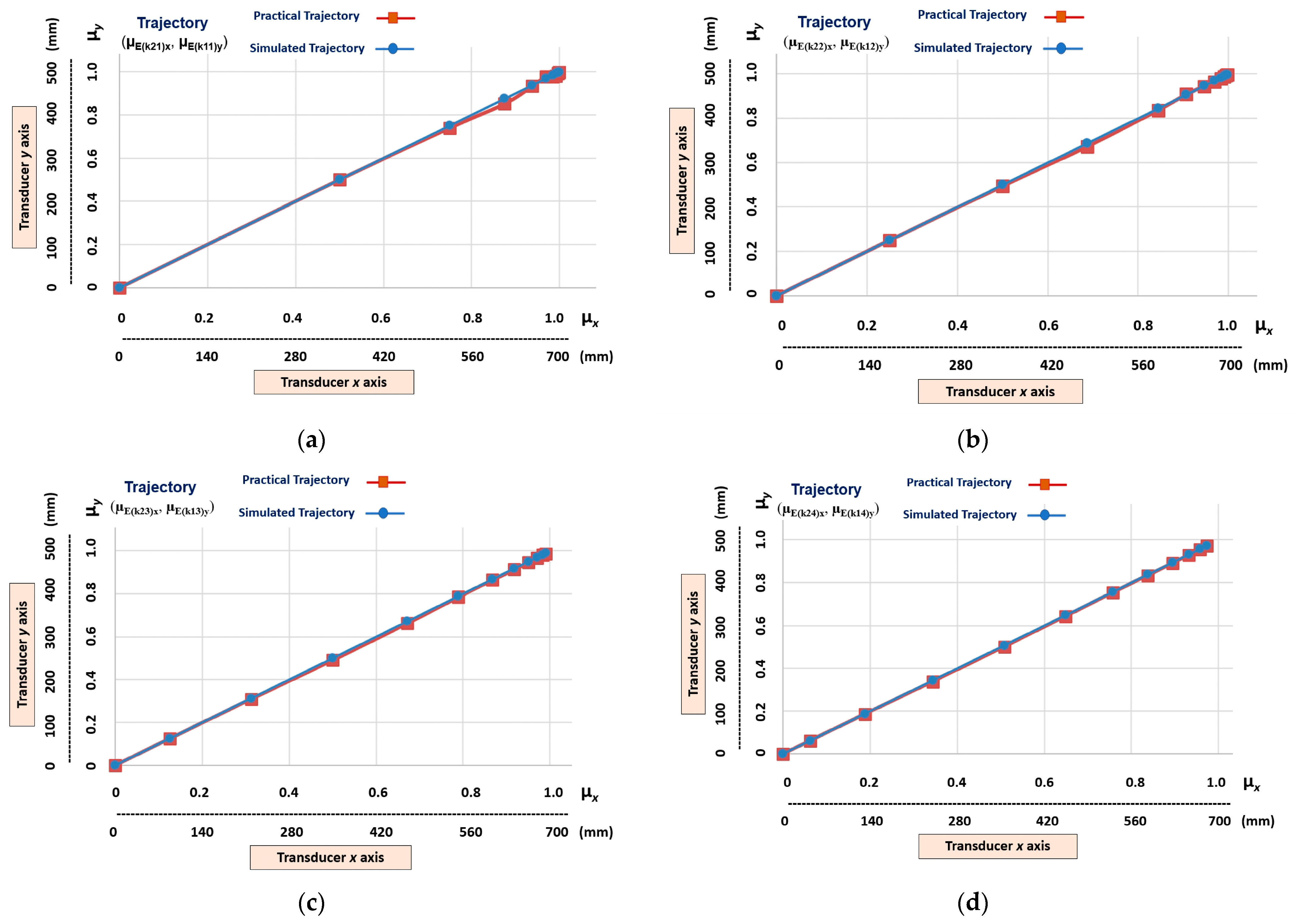
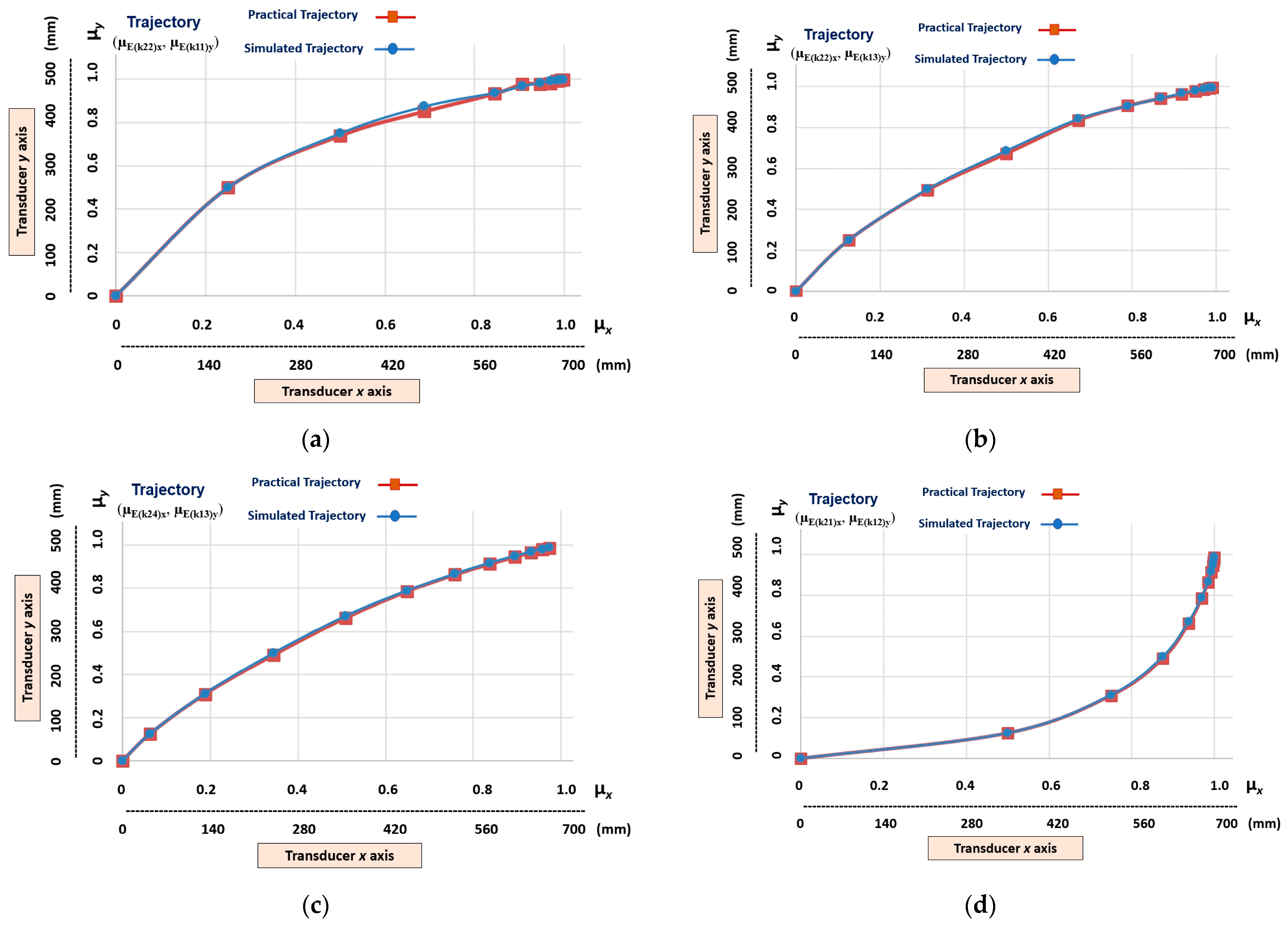
  • Linear trajectories (g1n), which are obtained at the outputs (µE(k21)x, µE(k11)y), (µE(k22)x, µE(k12)y), (µE(k23)x, µE(k13)y), and (µE(k24)x, µE(k14)y);
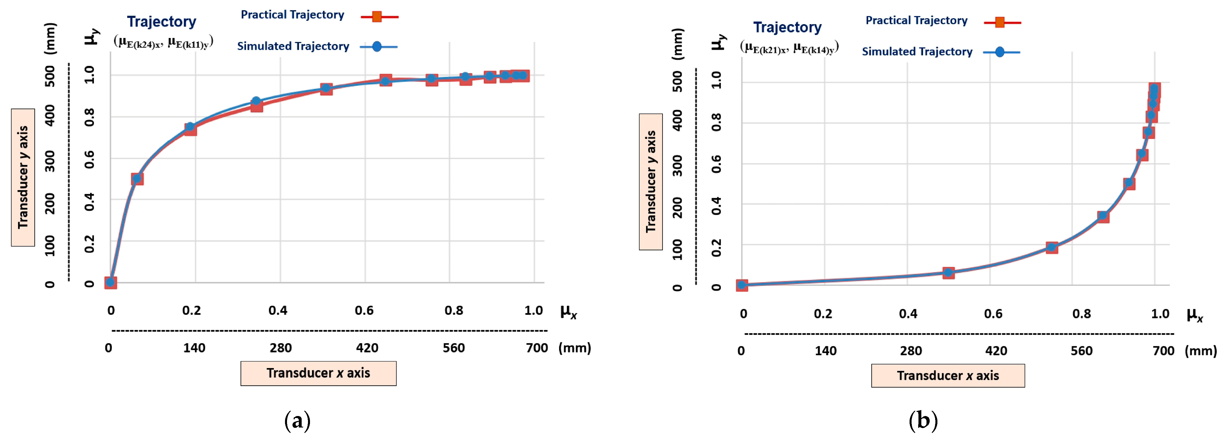
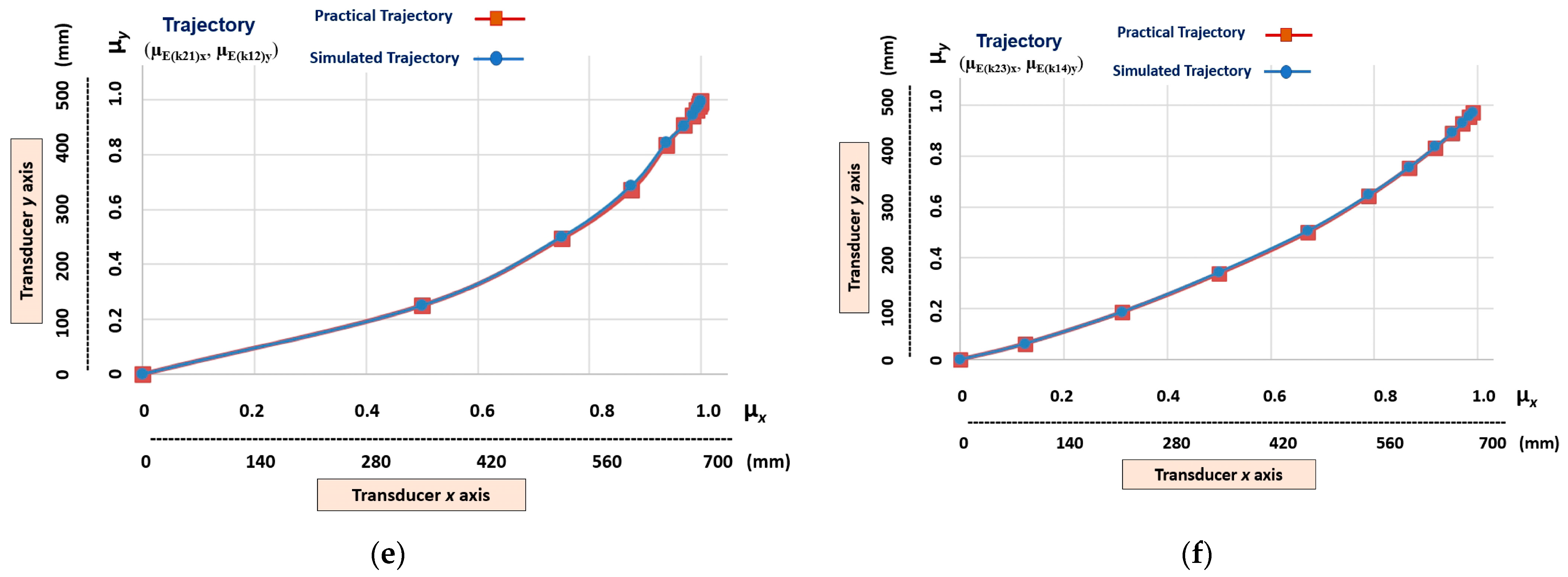
  • Non-linear trajectories that have a higher level of slope (gnlh), which are those obtained at the outputs (µE(k24)x, µE(k11)y) and (µE(k21)x, µE(k14)y);
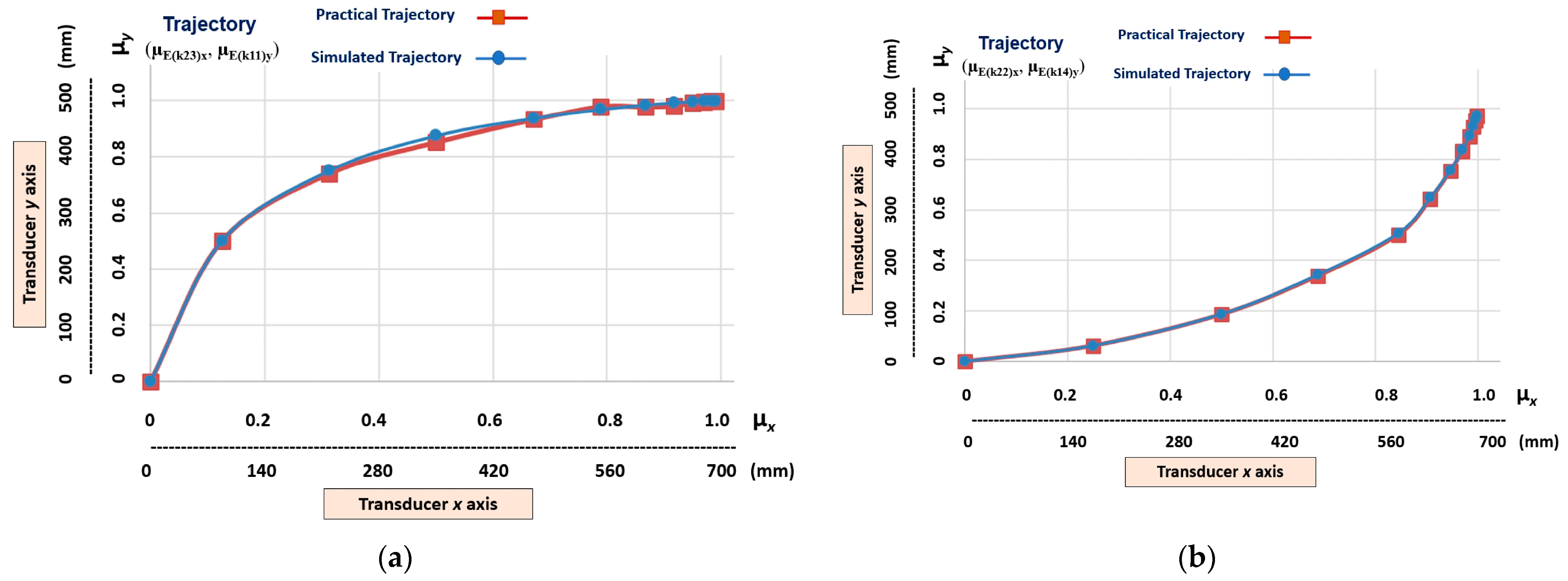
  • Non-linear trajectories that present a medium level of non-linearity (gnlm), which are those obtained at the outputs (µE(k23)x, µE(k11)y), (µE(k24)x, µE(k12)y), (µE(k22)x, µE(k14)y) and (µE(k21)x, µE(k13)y);
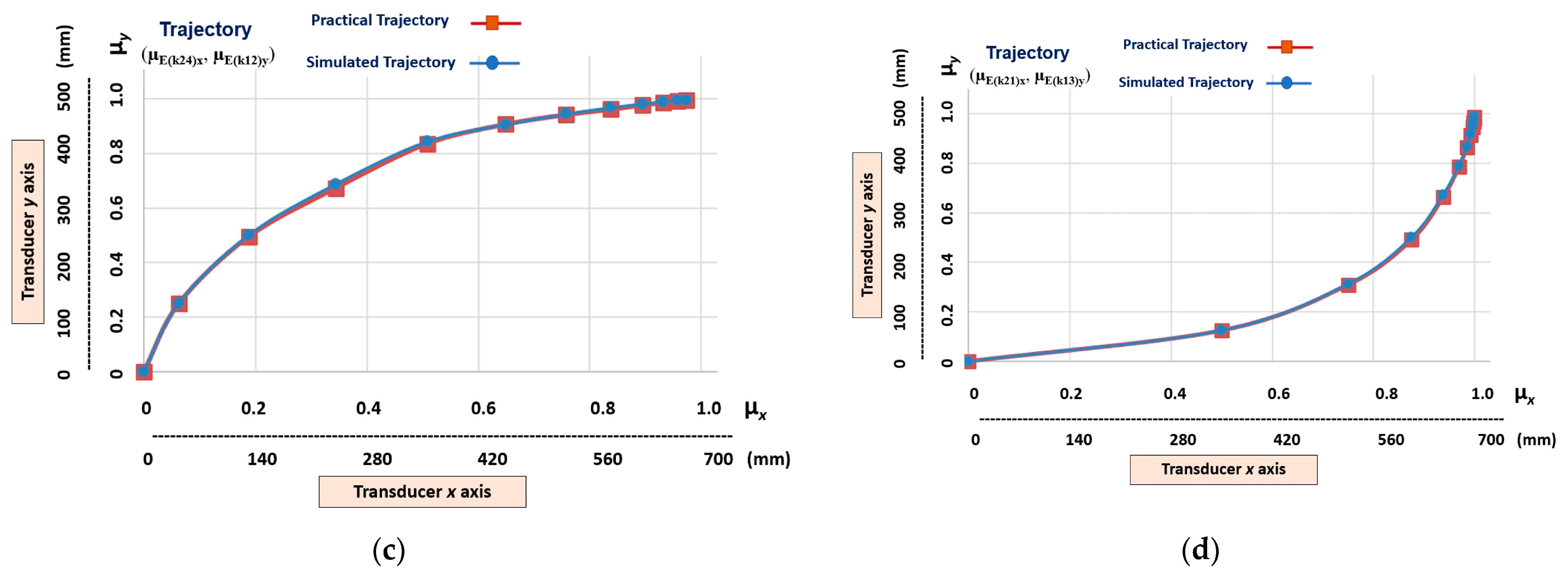
  • Non-linear trajectories that have a low level of non-linearity (gnll), which are those obtained at the outputs (µE(k22)x, µE(k11)y), (µE(k23)x, µE(k12)y), (µE(k24)x, µE(k13)y), (µE(k21)x, µE(k12)y), (µE(k22)x, µE(k13)y) and (µE(k23)x, µE(k14)y).

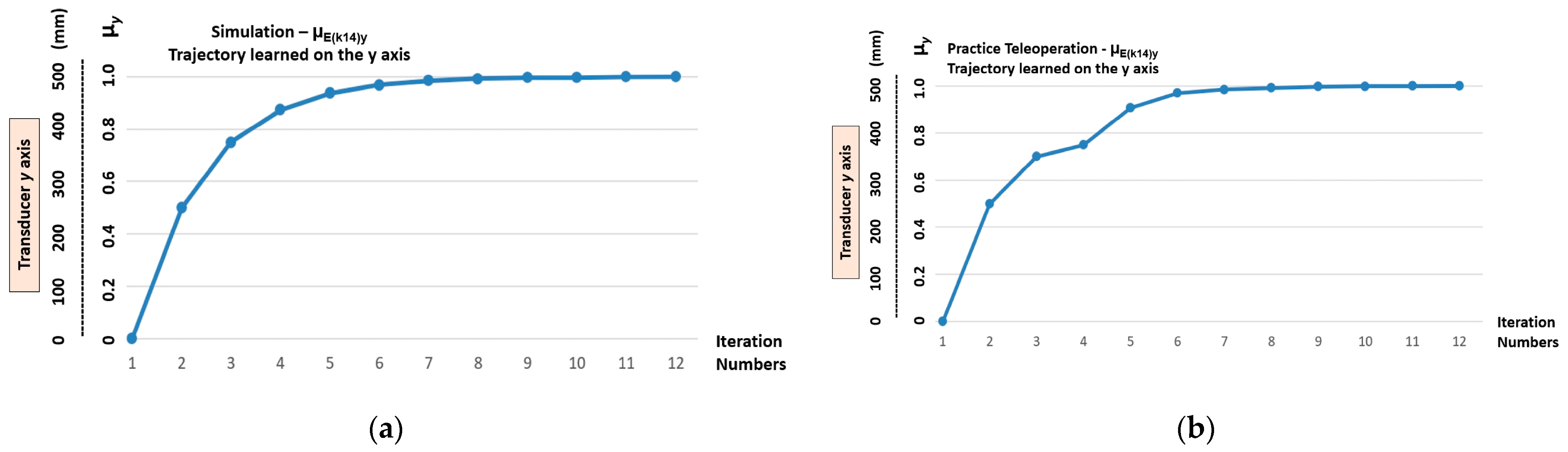
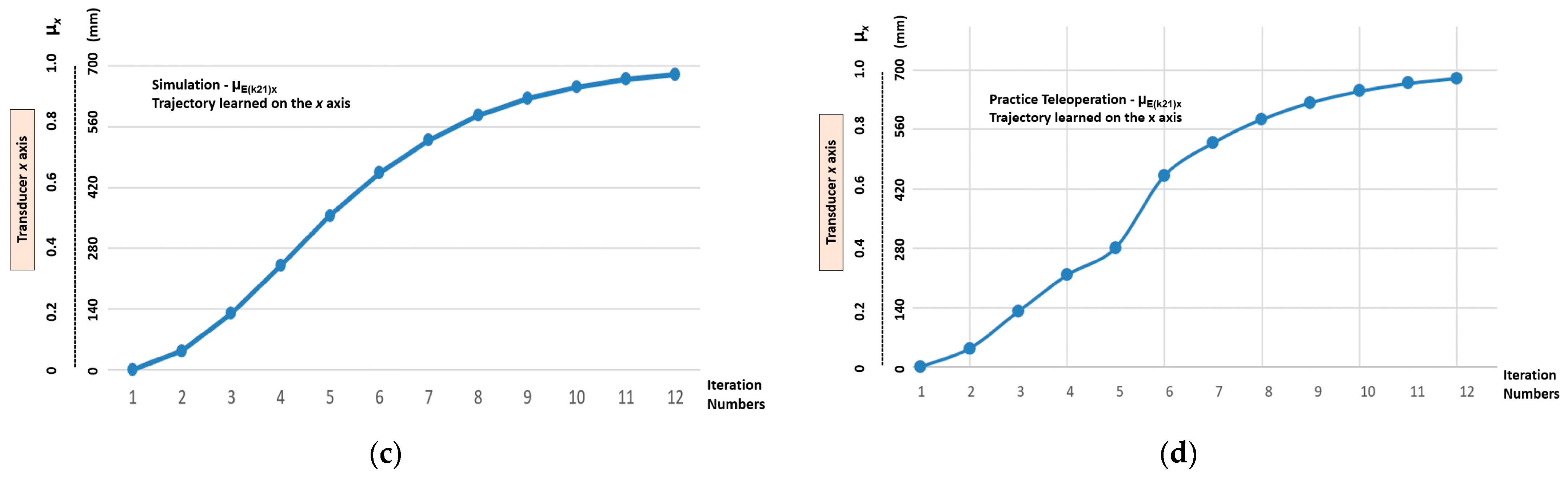
5.1. Learning Stage Results—Demonstration by Simulation

Initially, the structure that forms the lPANnet shown in Figure 9 was simulated to obtain the possible trajectories that could be learned by the linear Cartesian robot that acts on the machine tool. In the simulations of the lPANnet x and lPANnet y groups, the values of the patterns were applied directly to the input of the first cell programmed in the lPANC_BLK 1 function block. Initially, the pattern µ1 = 0 was applied until all outputs indicated zero (µ(k+1) = 0). Then, after applying 11 iterations of the unit pattern (µ1 = 1), the final condition of completed learning was considered.
Table 4 contains the values obtained in the learning process through simulation, and the outputs of all lPANC_BLK x and lPANC_BLK y blocks that make up the lPANnet are shown in Figure 9.
These values from Table 4, which were obtained by simulation, will be compared to the values obtained in practice, as shown below.

5.2. Learning Stage Results—Demonstration by Teleoperation

In the procedures performed for learning, the blocks were initially activated by teleoperation with a pattern of 0 in the first lPANCell until all outputs resulted in zero (µ(k+1) = 0). Then, through the button (joystick), the control system was manually activated n times to move the sliding crossbar cylinder along the length of the table in the x axis until the “learning completed” signal.
The patterns values applied to the input of the first cell programmed in lPANC_BLK 1x function block were obtained from the x-axis transducer. After the learning procedure for the x-axis, the cylinder of the mobile device movement with a magnetic grip on the y-axis was manually activated through the button (joystick) until the “learning completed” signal occurred. The patterns values applied to the input of the first cell programmed in lPANC_BLK 1y function block were obtained from the y-axis transducer.
Table 5 contains the values obtained in the learning process through teleoperation, and in the outputs of all lPANC_BLK x and lPANC_BLK y blocks that make up the lPANnet shown in Figure 9.
Figure 10 shows the graphical results of the learning stage of the 4 different linear trajectories learned by the Linear Cartesian robot of the machine tool. Trajectories represented by the transition states obtained in the outputs of the following cells (Figure 9): (μE(k21)x, μE(k11)y), (μE(k22)x, μE(k12)y), (μE(k23)x, μE(k13)y), and (μE(k24)x, μE(k14)y).
It can be seen in Figure 10 that, although the trajectories a, b, c, and d are linear, there are fundamental differences in the distances of their transition states. This indicates that each path has a different velocity.
Figure 11 shows the graphical results of the learning stage of the two different non-linear trajectories that have a higher level of slope. The trajectories learned by the linear Cartesian robot of the machine tool are represented by the transition states obtained in the outputs of the cells (Figure 9): (µE(k24)x, µE(k11)y) and (µE(k21)x, µE(k14)y).
Figure 12 shows the graphic results of the learning stage of the four different non-linear trajectories that have a medium level of slope. The trajectories learnt by the linear Cartesian robot of the machine tool are represented by the transition states obtained in the outputs of the following cells (Figure 9): (µE(k23)x, µE(k11)y), (µE(k22)x, µE(k14)y), (µE(k24)x, µE(k12)y), and (µE(k21)x, µE(k13)y).
Note, in Figure 12, that although the non-linear trajectories b and d are similar, there are fundamental differences in the distances of their transition states. This indicates that each trajectory has different velocities and accelerations.
Figure 13 shows the graphic results of the learning stage of the six different non-linear trajectories that have a low level of slope. The trajectories learned by the linear Cartesian robot of the machine tool are represented by the transition states obtained in the outputs of the following cells (Figure 9): (µE(k22)x, µE(k11)y), (µE(k22)x, µE(k13)y), (µE(k24)x, μE(k13)y), (µE(k21)x, μE(k12)y), (µE(k23)x, µE(k12)y), and (µE(k23)x, µE(k14)y).
Note, in Figure 13, that the nonlinear trajectories exhibit fundamental differences in the distances of their transition states. This indicates that each trajectory has different velocities and accelerations.

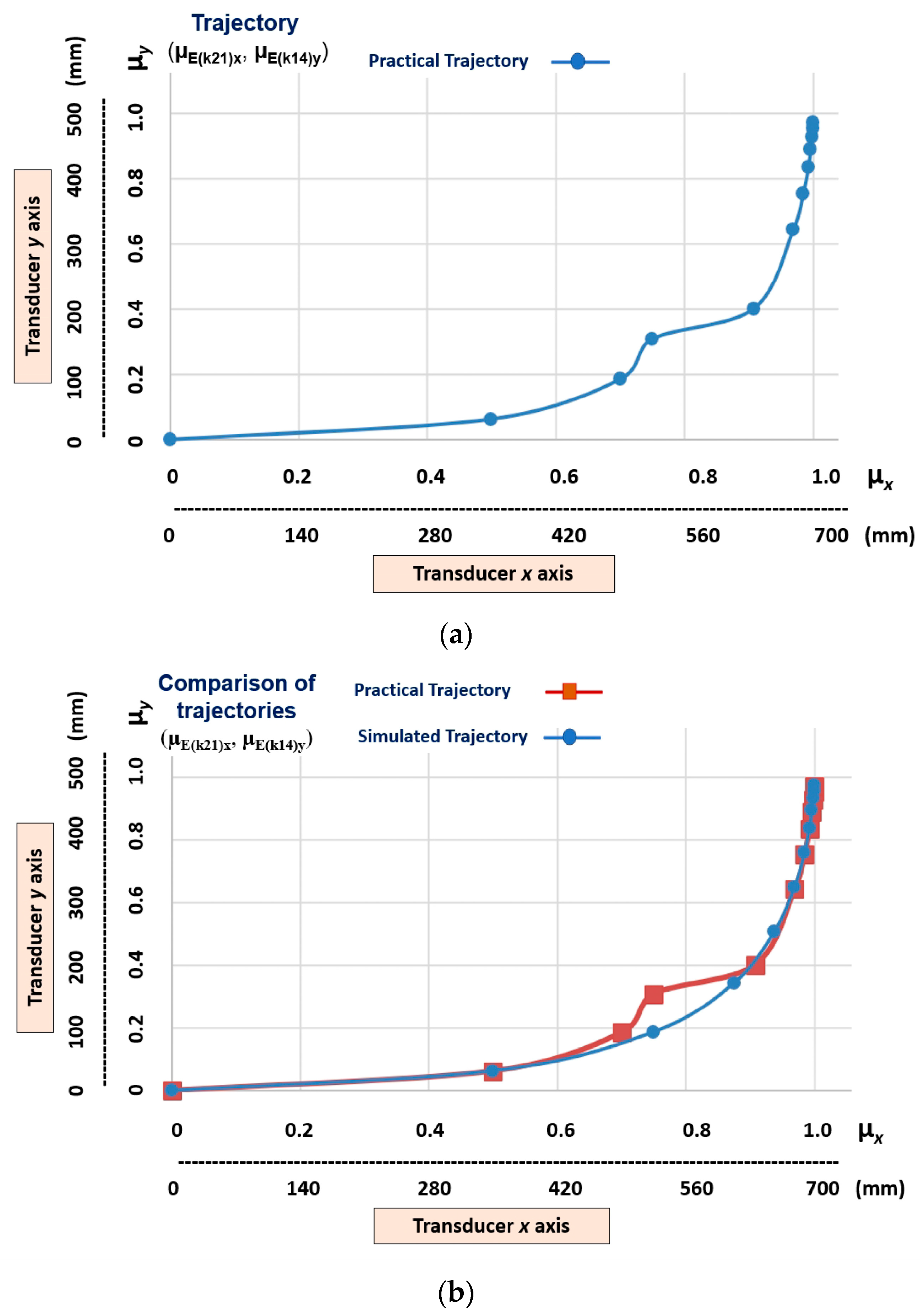
5.3. Imitation Step—Results

After the teleoperation learning stage, the linear Cartesian robot receives the signal (uE_Signaled) warning that the imitation action is available. In this imitation stage, the x and y axis transducers allow real-time monitoring. Therefore, in the operation of the machine tool moving the workpieces, the transducers provide information about the real-time trajectory that is being developed by the linear Cartesian robot.
Figure 14 shows the graphic results of the imitation stage that was performed by the linear Cartesian robot in a test on the gpn1 (µE(k24)x, µE(k11)y) trajectory, which was classified as the one with the highest level of nonlinearity.
Figure 15 shows the practical results compared to the simulated results.
As the graphs show in Figure 10, Figure 11, Figure 12 and Figure 13, the trajectories not only differ in linearity levels, but are also different in their relation to the distances between the transition states. This variation between the distances of the transition states in the trajectories indicates that the parameters of velocity and acceleration are intrinsic to the results. However, in this work, where the tests were performed in a linear Cartesian robot driven by pneumatic energy, these parameters were not possible to analyze.
The graphic results of the teleoperation learning stage showed that the linear Cartesian robot presented behaviors that were very close to the ideal results obtained by the simulation.
The graphical results shown in Figure 14 and Figure 15 indicate that, when learning the trajectory via teleoperation, a recognition problem occurred in the first transition states. This problem, presented in the learning stage, was reflected in the imitation stage. In the example (Figure 15b), we can see that in the third transition state the simulated and practical values are as follows:
Simulated Trajectory = (µE(k21)x, µE(k14)y) = (0.75, 0.1875);
  Practical Trajectory = (µE(k21)x, µE(k14)y) = (0.75, 0.3090).
When considering the simulated trajectory to be ideal, there is a maximum error of 64.8% in the practical trajectory toward the y axis. However, it appears that, both in the learning and imitation stage, the linear Cartesian robot showed that it has the conditions required to recover the ideal trajectory; this shows a robustness in the LfD process to disturbances that are carried out by the lPANCells being implemented in this type of configuration.

6. Conclusions

In this article, we present a way of applying Paraconsistent Logic to the method of learning by demonstration (LfD). Research on the LfD method has been developed with the objective of making a machine perform new tasks by imitating procedures that are presented to it, without the need for reconfiguration or for a reprogramming of its software. Paraconsistent Logic (PL) is non-classical logic that is capable of processing data with contradictory information. As shown in this work, algorithms that are built based on Paraconsistent Annotated Logic (PAL), which is an extension of PL, can open up promising paths in this area of knowledge. In this research, we used the Paraconsistent Artificial Neural Cell of Learning (lPANCell) algorithm, which responds well to learning normalized patterns that have values between 0 and 1 being applied repeatedly to its input function. Thus, through recurrence techniques, lPANCell is able to gradually store this information, thus presenting signals with asymptotic variation as an output response, which are controlled by an adjustment of a learning factor (lF). For the application of the LfD technique with PAL, an implementation of the lPANCell algorithm was made in a Programmable Controller (PC) in the form of a functional block called lPANC_BLK, which was available in a virtual library according to the IEC 61131-3 standard. The modularity of the lPANC_BLK functional block guarantees that it can be used in the formation of configurations that form Paraconsistent Artificial Neural Networks (lPANnet), which are used in industrial automation projects that involve Programmable Controllers. The practical results were obtained with several tests being carried out to validate the operation of a lPANCell operating in a network structure composed of 8 lPANCells that were acting in a learning from demonstration (LfD) process. The LfD method, with the proposed lPANCnet configuration, was tested in a linear Cartesian robot, which worked as a machine tool for moving metallic workpieces. The lPANnet paraconsistent structure dedicated to “Learning” and “Imitation” was divided into two sets of four functional blocks each: where one acts in the learning process of linear Cartesian robot on the x-axis, and the other acts in the learning process of linear Cartesian robot on the y axis. The LfD technique presented in this work was the learning by teleoperation variant, where, at the end of the procedures, transition states (Xn, Yn) for 16 trajectories of different linearity levels were created. The results obtained in the various tests carried out showed that the lPANnet configuration built with lPANC_BLK blocks is very efficient and responds adequately to all steps of the LfD process. This indicates that the lPANnet paraconsistent structure is able to provide learning dynamic properties; further, it has a robustness to disturbances that can be monitored in real time, both in the learning process by demonstration and in the imitation process. Based on the results obtained in this work, new studies will be conducted by applying other different configurations with paraconsistent neural networks (lPANnet) in the LfD process, thus covering more complex dynamic systems that are used in industrial plants and in the areas of robotics.

Author Contributions

Resources and formal analysis, J.I.D.S.F. and C.L.M.F.; methodology and investigation, R.S.d.S., P.M.G. and S.L.d.C.M.; software and conceptualization, L.d.E.S., V.C.N. and H.M.C.; original draft preparation, W.A.C.L., M.C.M. and D.V.G.; writing—review and editing, C.R.T. and J.M.A.; supervision, review and editing, G.L.-T. All authors have read and agreed to the published version of the manuscript.

Funding

This research received no external funding.

Institutional Review Board Statement

Not applicable.

Informed Consent Statement

Not applicable.

Data Availability Statement

Not applicable.

Conflicts of Interest

The authors declare no conflict of interest.

References

  1. Haefner, N.; Wincent, J.; Parida, V.; Gassmann, O. Artificial intelligence and innovation management: A review, framework, and research agenda. Technol. Forecast. Soc. Chang. 2021, 162, 120392. [Google Scholar] [CrossRef]
  2. Angeles, J. Fundamentals of Robotic Mechanical Systems: Theory, Methods, and Algorithms, 3rd ed.; Springer: New York, NY, USA, 2007; ISBN 978-3-319-01850-8. [Google Scholar] [CrossRef]
  3. Craig, J.J. Introduction to Robotics: Mechanics and Control, 4th ed.; Pearson: Toronto, ON, Canada, 2022; ISBN 9780137848744. [Google Scholar]
  4. Torres, C.R.; Lambert-Torres, G.; Abe, J.M.; Da Silva Filho, J.I. The sensing system for the autonomous mobile robot Emmy III. In Proceedings of the 2011 IEEE International Conference on Fuzzy Systems (FUZZ-IEEE 2011), Taipei, Taiwan, 27–30 June 2011; pp. 2928–2933. [Google Scholar] [CrossRef]
  5. Torres, C.R.; Abe, J.M.; Lambert-Torres, G.; Da Silva Filho, J.I.; Martins, H.G. A Sensing System for an Autonomous Mobile Robot Based on the Paraconsistent Artificial Neural Network. In Knowledge-Based and Intelligent Information and Engineering Systems; KES 2010; Lecture Notes in Computer Science; Setchi, R., Jordanov, I., Howlett, R.J., Jain, L.C., Eds.; Springer: Berlin/Heidelberg, Germany, 2010; Volume 6278. [Google Scholar] [CrossRef]
  6. Da Silva Filho, J.I.; Lambert-Torres, G.; Abe, J.M. Uncertainty Treatment Using Paraconsistent Logic—Introducing Paraconsistent Artificial Neural Networks; IOS Press: Amsterdam, The Netherlands, 2010; p. 320. ISBN 978-1-60750-557-0. [Google Scholar]
  7. Côrtes, H.M.; Santos, P.E.; Da Silva Filho, J.I. Monitoring electrical systems data-network equipment by means of Fuzzy and Paraconsistent Annotated Logic. Expert Syst. Appl. 2022, 187, 115865. [Google Scholar] [CrossRef]
  8. Ravichandar, H.; Polydoros, A.S.; Chernova, S.; Billard, A. Recent Advances in Robot Learning from Demonstration. Annu. Rev. Control Robot. Auton. Syst. 2020, 3, 297–330. [Google Scholar] [CrossRef]
  9. Argall, B.D.; Chernova, S.; Veloso, M.; Browning, B. A survey of robot learning from demonstration. Robot. Auton. Syst. 2009, 57, 469–483. [Google Scholar] [CrossRef]
  10. Verstaevel, N.; Régis, C.; Gleizes, M.P.; Robert, F. Principles and Experimentations of Self-Organizing Embedded Agents Allowing Learning From Demonstration in Ambient Robotics. Future Gener. Comput. Syst. 2016, 64, 78–87. [Google Scholar] [CrossRef]
  11. Ekvall, S.; Kragic, D. Robot learning from demonstration: A task-level planning approach. Int. J. Adv. Robot. Syst. 2008, 5, 223–234. [Google Scholar] [CrossRef]
  12. De Carvalho, A.; Da Silva Filho, J.I.; Mario, M.C.; Blos, M.F.; Da Cruz, C.M. A Study of Paraconsistent Artificial Neural Cell of Learning Applied as PAL2v Filter. IEEE Lat. Am. Trans. 2018, 16, 202–209. [Google Scholar] [CrossRef]
  13. Da Silva Filho, J.I.; da Cruz, C.M.; Rocco, A.; Garcia, D.V.; Ferrara, L.F.P.; Onuki, A.S.; Mario, M.C.; Abe, J.M. Paraconsistent Artificial Neural Network for Structuring Statistical Process Control in Electrical Engineering. In Towards Paraconsistent Engineering; Intelligent Systems Reference Library; Akama, S., Ed.; Springer: Cham, Stwitzerland, 2016; Volume 110. [Google Scholar] [CrossRef]
  14. Abe, J.M.; Torres, C.R.; Lambert-Torres, G.; Da Silva Filho, J.I.; Martins, H.G. Paraconsistent Autonomous Mobile Robot Emmy III. In Advances in Technological Applications of Logical and Intelligent Systems; Series Frontiers in Artificial Intelligence and Applications; IOS Press: Amsterdam, The Netherlands, 2009; Volume 186, pp. 236–258. [Google Scholar] [CrossRef]
  15. Nicolescu, M.N.; Mataric, M.J. Natural methods for robot task learning: Instructive demonstrations, generalization and practice. In Proceedings of the Second International Joint Conference on Autonomous Agents and Multiagent Systems, Melbourne, VIC, Australia, 14–18 July 2003; pp. 241–248. [Google Scholar]
  16. Billard, A.; Calinon, S.; Dillmann, R.; Schaal, S. Robot programming by demonstration. In Springer Handbook of Robotics; Siciliano, B., Khatib, O., Eds.; Springer: Berlin/Heidelberg, Germany, 2008; pp. 1371–1394. [Google Scholar]
  17. Mugan, J.; Kuipers, B. Autonomous learning of high-level states and actions in continuous environments. IEEE Trans. Auton. Ment. Dev. (TAMD) 2012, 4, 70–86. [Google Scholar] [CrossRef]
  18. Gienger, M.; Mühlig, M.; Steil, J.J. Imitating object movement skills with robots—A task-level approach exploiting generalization and invariance. In Proceedings of the 2010 IEEE/RSJ International Conference on Intelligent Robots and Systems, Taipei, Taiwan, 18–22 October 2010; pp. 1262–1269. [Google Scholar] [CrossRef]
  19. Mohseni-Kabir, A.; Rich, C.; Chernova, S.; Sidner, C.L.; Miller, D. Interactive hierarchical task learning from a single demonstration. In Proceedings of the Tenth Annual—ACM/IEEE International Conference on Human-Robot Interaction, HRI ’15, Portland, OR, USA, 2–5 March 2015; ACM: New York, NY, USA; pp. 205–212. [Google Scholar]
  20. Zimmerman, T.; Kambhampati, S. Learning-Assisted Automated Planning: Looking Back, Taking Stock, Going Forward. AI Mag. 2003, 24, 73. [Google Scholar] [CrossRef]
  21. Jiménez, S.; De La Rosa, T.; Fernández, S.; Fernández, F.; Borrajo, D. A review of machine learning for automated planning. Knowl. Eng. Rev. 2012, 27, 433–467. [Google Scholar] [CrossRef]
  22. Fikes, R.E.; Hart, P.E.; Nilsson, N.J. Learning and executing generalized robot plans. Artif. Intell. 1972, 3, 251–288. [Google Scholar] [CrossRef]
  23. Chrpa, L. Generation of macro-operators via investigation of action dependencies in plans. Knowl. Eng. Rev. 2010, 25, 281–297. [Google Scholar] [CrossRef]
  24. Hu, Y.; De Giacomo, G. Generalized planning: Synthesizing plans that work for multiple environments. In Proceedings of the IJCAI Proceedings-International Joint Conference on Artificial Intelligence, Catalonia, Spain, 16–22 July 2011; Volume 22, pp. 918–923. [Google Scholar]
  25. Zhuo, H.H.; Muñoz-Avila, H.; Yang, Q. Learning hierarchical task network domains from partially observed plan traces. Artif. Intell. 2014, 212, 134–157. [Google Scholar] [CrossRef]
  26. Ingrand, F.; Ghallab, M. Deliberation for autonomous robots: A survey. Artif. Intell. 2017, 247, 10–44. [Google Scholar] [CrossRef]
  27. Abe, J.M.; Da Silva Filho, J.I. Manipulating conflicts and uncertainties in robotics. J. Mult.-Valued Log. Soft Comput. 2003, 9, 147–169. [Google Scholar]
  28. De Carvalho, A.; Justo, J.F.; Angelico, B.A.; De Oliveira, A.M.; Da Silva Filho, J.I. Rotary Inverted Pendulum Identification for Control by Paraconsistent Neural Network. IEEE Access 2021, 9, 74155–74167. [Google Scholar] [CrossRef]
  29. Pastor, P.; Kalakrishnan, M.; Meier, F.; Stulp, F.; Buchli, J.; Theodorou, E.; Schaal, S. From dynamic movement primitives to associative skill memories. Robot. Auton. Syst. 2013, 61, 351–361. [Google Scholar] [CrossRef]
  30. Ijspeert, A.J.; Nakanishi, J.; Schaal, S. Movement imitation with nonlinear dynamical systems in humanoid robots. In Proceedings of the IEEE International Conference on Robotics and Automation (ICRA2002), Washington, DC, USA, 11–15 May 2002; pp. 1398–1403. [Google Scholar]
  31. Ijspeert, A.J.; Nakanishi, J.; Schaal, S. Learning rhythmic movements by demonstration using nonlinear oscillators. In Proceedings of the IEEE/RSJ International Conference on Intelligent Robots and Systems (IROS2002), EPFL, Lausanne, Switzerland, 30 September–4 October 2002; pp. 958–963. [Google Scholar]
  32. Zhu, Z.; Hu, H. Robot Learning from Demonstration in Robotic Assembly: A Survey. Robotics 2018, 7, 17. [Google Scholar] [CrossRef]
  33. Aleotti, J.; Caselli, S.; Reggiani, M. Leveraging on a virtual environment for robot programming by demonstration. Robot. Auton. Syst. 2004, 47, 153–161. [Google Scholar] [CrossRef]
  34. Schaal, S. Dynamic movement primitives—A framework for motor control in humans and humanoid robotics. In Adaptive Motion of Animals and Machines; Springer: Tokio, Japan, 2006; pp. 261–280. [Google Scholar]
  35. Niekum, S.; Osentoski, S.; Konidaris, G.; Chitta, S.; Marthi, B.; Barto, A.G. Learning grounded finite-state representations from unstructured demonstrations. Int. J. Robot. Res. 2015, 34, 131–157. [Google Scholar] [CrossRef]
  36. Sosa-Ceron, A.D.; Gonzalez-Hernandez, H.G.; Reyes-Avendaño, J.A. Learning from Demonstrations in Human–Robot Collaborative Scenarios: A Survey. Robotics 2022, 11, 126. [Google Scholar] [CrossRef]
  37. Sarker, I.H. Machine Learning: Algorithms, Real-World Applications and Research Directions. SN Comput. Sci. 2021, 2, 160. [Google Scholar] [CrossRef]
  38. Akbari, E.; Mir, M.; Vasiljeva, M.V.; Alizadeh, A.; Nilashi, M. A Computational Model of Neural Learning to Predict Graphene Based ISFET. J. Electron. Mater. 2019, 48, 4647–4652. [Google Scholar] [CrossRef]
  39. Liu, T.; Lemeire, J. Efficient and Effective Learning of HMMs Based on Identification of Hidden States. Math. Probl. Eng. 2017, 2017, 7318940. [Google Scholar] [CrossRef]
  40. Kulić, D.; Ott, C.; Lee, D.; Ishikawa, J.; Nakamura, Y. Incremental learning of full body motion primitives and their sequencing through human motion observation. Int. J. Robot. Res. 2012, 31, 330–345. [Google Scholar] [CrossRef]
  41. Ijspeert, A.J.; Nakanishi, J.; Hoffmann, H.; Pastor, P.; Schaal, S. Dynamical Movement Primitives: Learning Attractor Models for Motor Behaviors. Neural Comput. 2013, 25, 328–373. [Google Scholar] [CrossRef]
  42. Guo, W.; Li, R.; Cao, C.; Gao, Y. Kinematics, dynamics, and control system of a new 5-degree-of-freedom hybrid robot manipulator. Adv. Mech. Eng. 2016, 8, 11. [Google Scholar] [CrossRef]
  43. Chi, M.; Yao, Y.; Liu, Y.; Zhong, M. Learning, Generalization, and Obstacle Avoidance with Dynamic Movement Primitives and Dynamic Potential Fields. Appl. Sci. 2019, 9, 1535. [Google Scholar] [CrossRef]
  44. Abe, J.M.; Lopes, H.F.D.S.; Anghinah, R. Paraconsistent artificial neural networks and Alzheimer disease: A preliminary study. Dement. Neuropsychol. 2007, 1, 241–247. [Google Scholar] [CrossRef]
  45. Kurfess, T.R. (Ed.) Robotics and Automation Handbook; CRC Press LLC.: Boca Raton, FL, USA, 2005. [Google Scholar]
  46. Sanchez-Sanchez, P.; Reyes-Cortes, F. Cartesian Control for Robot Manipulators. In Robot Manipulators Trends and Development; Jimenez, A., Al Hadithi, B.M., Eds.; IntechOpen: London, UK, 2010. [Google Scholar] [CrossRef]
  47. Cuesta, R.; Alvarez, J.; Miranda, M. Robust Tracking and Cruise Control of a Class of Robotic Systems. Math. Probl. Eng. 2015, 2015, 728412. [Google Scholar] [CrossRef]
  48. Da Costa, N.C.A.; Abe, J.M.; Subrahmanian, V.S. Remarks on annotated logic. Z. Math. Logik Grundl. Math. 1991, 37, 561–570. [Google Scholar]
  49. Garcia, D.V.; Da Silva Filho, J.I.; Silveira, L.; Pacheco, M.T.T.; Abe, J.M.; Carvalho, A.; Blos, M.F.; Pasqualucci, C.A.G.; Mario, M.C. Analysis of Raman spectroscopy data with algorithms based on paraconsistent logic for characterization of skin cancer lesions. Vib. Spectrosc. 2019, 103, 102929. [Google Scholar] [CrossRef]
  50. Da Silva Filho, J.I.; Abe, J.M.; Marreiro, A.D.L.; Martinez, A.A.G.; Torres, C.R.; Rocco, A.; Côrtes, H.M.; Mario, M.C.; Pacheco, M.T.T.; Garcia, D.V.; et al. Paraconsistent Annotated Logic Algorithms Applied in Management and Control of Communication Network Routes. Sensors 2021, 21, 4219. [Google Scholar] [CrossRef]
  51. Coelho, M.S.; Da Silva Filho, J.I.; Côrtes, H.M.; de Carvalho, A.; Blos, M.F.; Mario, M.C.; Rocco, A. Hybrid PI controller constructed with paraconsistent annotated logic. Control Eng. Pract. 2019, 84, 112–124. [Google Scholar] [CrossRef]
  52. Da Silva Filho, J.I.; de Oliveira, R.A.B.; Rodrigues, M.C.; Côrtes, H.M.; Rocco, A.; Mario, M.C.; Garcia, D.V.; Abe, J.M.; Torres, C.R.; Ricciotti, V.B.D.; et al. Predictive Controller Based on Paraconsistent Annotated Logic for Synchronous Generator Excitation Control. Energies 2023, 16, 1934. [Google Scholar] [CrossRef]
  53. Ferrara, L.F.P.; Yamanaka, K.; Da Silva Filho, J.I. A system of recognition of characters based on paraconsistent artificial neural networks. Front. Artif. Intell. Appl. 2005, 132, 127–134. [Google Scholar]
  54. John, K.H.; Tiegelkamp, M. IEC61131-3: Programing Industrial Automation Systems: Concepts and Programming Languages, Requirements for Programing Systems, Decision—Making Aids, 2nd ed.; Springer: New York, NY, USA, 2010; 390p. [Google Scholar]
  55. Salih, H.; Abdelwahab, H.; Abdallah, A. Automation design for a syrup production line using Siemens PLC S7-1200 and TIA Portal software. In Proceedings of the 2017 International Conference on Communication, Control, Computing and Electronics Engineering (ICCCCEE), Khartoum, Sudan, 16–18 January 2017; pp. 1–5. [Google Scholar] [CrossRef]
Figure 1. Block diagram of supervised learning.
Robotics 12 00069 g001
Figure 2. Unit Square in the Cartesian plane (USCP) with the evidence degrees µ and λ, and the PAL lattice with a paraconsistent logic state composed by the pair (Dc, Dct).
Robotics 12 00069 g002
Figure 3. Symbol of the lPANCell and the graphs with the curves corresponding to the outputs (μ(k+1)), which were obtained with 12 iterations of the pattern μ1 = 1 with lF = 1, lF = 0.8, lF = 0.6, lF = 0.4, and lF = 0.2.
Robotics 12 00069 g003
Figure 4. Answers in the form of graphs of the Paraconsistent Artificial Neural Cell of Learning (lPANCell), adjusted with lF = 1 in the sequential application of 5 patterns with different values, with 10 iterations each.
Robotics 12 00069 g004
Figure 5. Structure of the Paraconsistent Artificial Neural Network with lPANCells interconnected in a cascade. (a) lPANnet configuration with cascading learning cells. (b) Graphical results obtained from the patterns learned in the outputs of the four lPANCells.
Robotics 12 00069 g005
Figure 6. Symbol of lPANC_BLK function block and the corresponding nomenclatures used with the lPANCell symbol.
Robotics 12 00069 g006
Figure 7. Linear Cartesian robot (gantry robot) acting on a pneumatic machine tool that has the task of moving metal workpieces.
Robotics 12 00069 g007
Figure 8. The linear Cartesian robot drive control system used in the process of moving metallic workpieces.
Robotics 12 00069 g008
Figure 9. Structure of the Paraconsistent Artificial Neural Network that was applied in a learning from demonstration (LfD) framework to the linear Cartesian robot, with possibilities to select up to 16 trajectories in the x and y axes.
Robotics 12 00069 g009
Figure 10. The graphic results of the linear Cartesian robot learning the linear trajectories. (a) Transition states (µE(k21)x, µE(k11)y). (b) Transition states (µE(k22)x, µE(k12)y). (c) Transition states (µE(k23)x, µE(k13)y). (d) Transition states (µE(k24)x, µE(k14)y).
Robotics 12 00069 g010
Figure 11. The graphic results of the linear Cartesian robot learning the non-linear trajectories with a higher level of slope. (a) Transition states (μE(k24)x, μE(k11)y). (b) Transition states (μE(k22)x, μE(k12)y).
Robotics 12 00069 g011
Figure 12. The graphic results of the linear Cartesian robot learning the non-linear trajectories with a medium level of slope. (a) Transition states (µE(k23)x, µE(k11)y). (b) Transition states (µE(k22)x, µE(k14)y). (c) Transition states (µE(k24)x, µE(k12)y). (d) Transition states (µE(k21)x, µE(k13)y).
Robotics 12 00069 g012aRobotics 12 00069 g012b
Figure 13. The graphic results of the linear Cartesian robot learning the non-linear trajectories with a low level of slope. (a) Transition states (µE(k22)x, µE(k11)y). (b) Transition states (µE(k22)x, µE(k13)y). (c) Transition states (µE(k24)x, µE(k13)y). (d)Transition states (µE(k21)x, µE(k12)y). (e) Transition states (µE(k23)x, µE(k12)y). (f) Transition states (µE(k23)x, µE(k14)y).
Robotics 12 00069 g013aRobotics 12 00069 g013b
Figure 14. The graphic results of the imitation step after the linear Cartesian robot having learnt the trajectory (μE(k21)x, μE(k14)y) with the highest level of nonlinearity. (a) Y-axis trajectory—μE(k14)y output learnt via simulation. (b) Y-axis trajectory—μE(k14)y output learnt via teleoperation. (c) X-axis trajectory—μE(k21)x learnt via simulation. (d) X-axis trajectory—μE(k21)x output learnt via teleoperation.
Robotics 12 00069 g014aRobotics 12 00069 g014b
Figure 15. The graphic practical results compared to the simulated results. (a) Trajectory with the x and y axes—outputs of the transition states (µE(k21)x, µE(k14)y) learnt via teleoperation. (b) Comparison between the trajectory learnt via teleoperation and the trajectory learnt via simulation.
Robotics 12 00069 g015
Table 1. Symbols and abbreviations.
Symbols/AbbreviationsMeaning
PLParaconsistent Logic
LfDLearning from Demonstration process
PALParaconsistent Annotated Logic
PAL2vParaconsistent Annotated Logic with Annotation of Two Values
PANCellParaconsistent Artificial Neural Cell
lPANCelLearning Paraconsistent Artificial Neural Cell
lPANnetParaconsistent Artificial Neural Network
lPANC_BLKParaconsistent Artificial Neural Cell Programmed with IEC 61131-3 Rules as Functional Block
HMMHidden Markov Models
DMPDynamic Motion Primitives
μFavorable Evidence Degree
λUnfavorable Evidence Degree
(μ, λ)Annotation of Two Values
USCPUnit Square in the Cartesian Plane
PProposition
tTrue Logical State
fFalse Logical State
Paracomplete Logical State
TInconsistent Logical State
DcCertainty Degree
DctContradiction Degree
DCRCertainty Degree of Real Value
μERResulting Evidence Degree
l F Learning Factor
Table 2. Values in the output (μ(k+1)) of the Paraconsistent Artificial Neural Cell of Learning (lPANCell) model, adjusted with lF = 1 in the sequential application of five patterns of different values, with 10 iterations each [6].
Pattern 1μ(k+1)Pattern 2μ(k+1)Pattern 3μ(k+1)Pattern 4μ(k+1)Pattern 5μ(k+1)
μ100.5μ110.50048828μ10.40.6995122μ10.80.60029249μ110.89980497
μ200.25μ210.75024414μ20.40.5497561μ20.80.70014625μ210.94990249
μ300.125μ310.87512207μ30.40.47487805μ30.80.75007312μ310.97495124
μ400.0625μ410.93756104μ40.40.43743902μ40.80.77503656μ410.98747562
μ500.03125μ510.96878052μ50.40.41871951μ50.80.78751828μ510.99373781
μ600.015625μ610.98439026μ60.40.40935976μ60.80.79375914μ610.99686891
μ700.0078125μ710.99219513μ70.40.40467988μ70.80.79687957μ710.99843445
μ800.0039062μ810.99609756μ80.40.40233994μ80.80.79843979μ810.99921723
μ900.0019531μ910.99804878μ90.40.40116997μ90.80.79921989μ910.99960861
μ1000.0009765μ1010.99902439μ100.40.40058498μ100.80.79960995μ1010.99980431
Table 3. Values of the results obtained in the training process of the configuration with four lPANCells interconnected in a cascade, as shown in Figure 5a.
Pattern 1 μ(k+n)μ(kn1) = Pattern 2μ(kn2) = Pattern 3μ(kn3) = Pattern 4 μ(kn4)
μ100000
μ210.50.250.1250.0625
μ310.750.50.31250.1875
μ410.8750.68750.50.34375
μ510.93750.843750.6718750.507813
μ610.968750.906250.7890630.648438
μ710.9843750.9453130.8671880.757813
μ810.99218750.968750.9179690.837891
μ910.996093750.9824220.9501950.894043
μ1010.998046880.9902340.9702150.932129
μ1110.999023440.9946290.9824220.957275
μ1210.999511720.997070.9897460.973511
Table 4. Values obtained through simulation of the outputs from the lPANC_BLK x and lPANC_BLK y blocks that make up the lPANCnet that are shown in Figure 9.
Simulation Results—x-Axis (X0)—lPANC_BLK xSimulation Results—y-Axis (Y0)—lPANC_BLK y
μE(k21)xμE(k22)xμE(k23)xμE(k24)xμE(k11)yμE(k12)yμE(k13)yμE(k14)y
μ100000000
μ20.50000000.2500000.125000.0625000.50000000.2500000.1250000.062500
μ30.75000000.5000000.312500.1875000.75000000.5000000.3125000.187500
μ40.87500000.6875000.500000.3437500.87500000.6875000.5000000.343750
μ50.93750000.8437500.6718750.5078130.93750000.8437500.6718750.507813
μ60.96875000.9062500.7890630.6484380.96875000.9062500.7890630.648438
μ70.98437500.9453130.8671880.7578130.98437500.9453130.8671880.757813
μ80.99218750.9687500.9179690.8378910.99218750.9687500.9179690.837891
μ90.996093750.9824220.9501950.8940430.996093750.9824220.9501950.894043
μ100.998046880.9902340.9702150.9321290.998046880.9902340.9702150.932129
μ110.999023440.9946290.9824220.9572750.999023440.9946290.9824220.957275
μ120.999511720.9970700.9897460.9735110.999511720.9970700.9897460.973511
Table 5. Values obtained through teleoperation in the outputs of the lPANC_BLK x and lPANC_BLK y blocks that make up the lPANnet shown in Figure 9.
Teleoperation Results—x-Axis (X0)—lPANC_BLK xTeleoperation Results—y-Axis (Y0)—lPANC_BLK y
μE(k21)xμE(k22)xμE(k23)xμE(k24)xμE(k11)yμE(k12)yμE(k13)yμE(k14)y
μ100000000
μ20.5000000.2500000.1250000.0625000.5000000.2500000.1250000.062500
μ30.7500000.5000000.3125000.1875000.7400000.4950000.3100000.186250
μ40.8750000.6875000.5000000.3437500.8520000.6735000.4917500.339000
μ50.9375000.8437500.6718750.5078130.9335000.8367500.6642500.501625
μ60.9687500.9062500.7890630.6484380.9787500.9077500.7860000.643813
μ70.9843750.9453130.8671880.7578130.9783750.9430630.8645310.754172
μ80.99218750.9687500.9179690.8378910.98218750.9626250.9135780.833875
μ90.99609380.9824220.9501950.8940430.99409380.9783590.9459690.889922
μ100.99804690.9902340.9702150.9321290.99704690.9877030.9668360.928379
μ110.99902340.9946290.9824220.9572750.99902340.9933630.9801000.954239
μ120.999311720.9969700.9896960.9734860.999811720.9965870.9883440.971291
Disclaimer/Publisher’s Note: The statements, opinions and data contained in all publications are solely those of the individual author(s) and contributor(s) and not of MDPI and/or the editor(s). MDPI and/or the editor(s) disclaim responsibility for any injury to people or property resulting from any ideas, methods, instructions or products referred to in the content.

