Positioning Control of Robotic Manipulators Subject to Excitation from Non-Ideal Sources

Abstract

The present work proposes the use of a hybrid controller combining concepts of a PID controller with LQR and a feedforward gain to control the positioning of a 2 DOF robotic arm with flexible joints subject to non-ideal excitations. To characterize the performance of the controls, two cases were studied. The first case considered the positioning control of the two links in fixed positions, while the second case considered the situation in which the second link is in rotational movement and the first one stays in a fixed position, representing a system with a non-ideal excitation source. In addition to the second case, the sensitivity of the proposed controls for changes in the length and mass of the second link in the rotational movement was analyzed. The results of the simulations showed the effectiveness of the controls, demonstrating that the PID control combined with feedforward gain provides the lowest error for both cases studied; however, it is sensitive to variations in the mass of the second link, in the case of rotational movements. The numerical results also revealed the effectiveness of the PD control obtained by LQR, presenting results similar to the PID control combined with feedforward gain, demonstrating the importance of the optimal control design.

1. Introduction

Robotic arms can be considered anthropomorphic robotic devices, due to their similarity with the human arm. They are formed of rigid links interconnected by joints and intended to function like a human arm, but with greater resistance and payload capacity. Such devices have been applied since their development to replace human work in carrying out dangerous activities in inaccessible places and in cases where repetitive tasks need to be performed during a certain period [1,2].

The trend is that, in the future, the use of robots as a workforce will grow, not only in industrial environments but also in other sectors of society. Industrial applications of robotic manipulators comprehend painting, welding, assembly, and precise positioning, among other skills. The applications in areas other than the industrial environment include underwater exploration, medical applications, such as assisted surgery, handling radioactive materials, and those with a risk of biological contamination, in the aerospace area, just to name a few [3,4].

Robotic manipulators are mechanical systems programmed to manipulate objects in a given space, obeying performance criteria and with a high degree of autonomy. However, the control of these devices is a challenging task, as they are non-linear, complex, and highly coupled dynamic systems.

Considering the non-linear and complex couplings inherent in robotic manipulators, Saleem et al. [5] proposed a new design of a linear quadratic integral regulator (LQIR) of complex fractional order (CFO), aiming to increase the robustness of inverted pendulum robotic mechanisms against limited exogenous perturbations. Experimental results demonstrated the described control’s effectiveness (CFO-LQIR) compared to their integer and fractional order counterparts. In Ali et al. [6], a robust control algorithm with an integral sliding mode control (ISMC) was suggested for a robotic arm with five degrees of freedom (DOF). The proposed nonlinear control considered friction compensation using the LuGre model. Numerical simulations using the Matlab/Simulink environment and experimental results on an autonomous articulated robot, developed internally on an educational platform (AUTAREP) and NI myRIO hardware interfaced with Lab-VIEW, were presented to demonstrate the effectiveness of the proposed control in trajectory tracking. Ali et al. [7] described a control algorithm in their work, combining the fast integral sliding mode control (FIT-SMC), with a robust exact differentiator observer (RED) and an estimator based on a feedforward neural network (FFNN). Numerical simulations for a robotic manipulator with 5 degrees of release, including joint friction modeled by LuGre friction, were presented. The numerical results demonstrated the efficacy of the control proposed by the authors for the robotic system with friction compensation and with an overshoot and a stabilization time of less than 1.5% and 0.2950 s, respectively, for all joints of the robotic manipulator considered. In Asghar et al. [8] the control techniques of a linear quadratic regulator (LQR) and proportional integral (PI) and integral (I) were analyzed and compared, for the positioning control of a serial robotic manipulator with 4 DOF. Numerical results were presented for comparison. In Rezoug et al. [9], a non-singular terminal sliding mode controller was proposed using an optimization technique with a hybrid metaheuristic method, for a robotic manipulator with 3 DOF. Numerical simulations were presented, demonstrating the effectiveness of the proposed control in tracking trajectories in the presence of disturbances and control uncertainties.

The case of robotic manipulators with 2 DOF degrees of freedom is a classic control problem, and, due to the widespread use of this type of robot in an industrial environment, this class is the subject of much research in the field of control and robotics. Over the years, many control strategies have been developed to control these devices and are reported in the literature and practical applications [10,11,12].

In their study, Zakia et al. [13] present a combination of sliding mode control (SMC) and PID control. Since PID control adjusts for system errors, SMC control ensures fast convergence. This hybrid controller provides greater system stability and the simulation results showed that the SMC–PID controller performed well in controlling the trajectory of the robotic arm.

In the work by Van et al. [14] a controller based on a fuzzy PID control and self-tuning SMC, and a time delay estimate (TDE) was proposed. Based on the results obtained, the authors state that, with fuzzy logic, the PID controller gains are effectively selected and that the integration of the TDE helps to eliminate prior knowledge of the exact dynamics of the system, in addition to reducing the computational load.

In studies by Rad et al. [15] and Yang et al. [16], adaptive control was used for robotic manipulators. In both studies, simulation results showed that the proposed controllers performed well, in addition to advantages such as lower sampling rate and tracking control with high precision and robustness.

In Korayem et al. [17,18,19,20] the non-linear controller SDRE (state-dependent Riccati equation) was applied to control a robotic manipulator with flexible joints. The simulation results showed that the SDRE method is suitable for solving ideal closed-loop nonlinear control problems, and, when comparing the method with the LQR controller, the SDRE controller presented a better performance.

In Lima et al. [21] a feedback control was obtained through the SDRE method (state-dependent Riccati equation) to reduce the vibration of the flexible link of a robotic manipulator. The simulation results showed that the proposed controller was more efficient for controlling vibrations when compared to the control provided only by the motors. Lima et al. [22] designed and analyzed a robotic arm with two degrees of freedom with flexible joints driven by a direct current motor (DC motor). To ease movement difficulties, magnetorheological dampers (MR damper) were attached to the links of the arm to provide a way to adjust the mechanical limitations of the arm. To control the positioning of the manipulator and the torque applied to the MR damper, a feedback control was developed through the state-dependent Riccati equation (SDRE). The simulation results demonstrated that the combined use of a DC motor and an MR damper was effective in controlling the position and behavior of the manipulator’s flexible joints. In Lima et al. [23,24], SDRE control was designed for a robotic manipulator with two degrees of freedom and a non-ideal excitation source. In addition to the control design, an MR brake has been included in the jousting. Numerical simulations demonstrated the efficiency of the studied control.

When interactions occur between dynamic systems, whether mechanical or not, oscillatory responses are produced. This kind of phenomenon has been comprehensively studied in the literature on systems with ideal excitation, in which the energy source is unlimited and depends only on the time. In the case of systems with nonideal sources (NIS), there is a dependency on the properties of the excitation source, whose energy is limited. This system has a source of linear excitation when the coupling of the equations does not have linear terms.

Although theories about dynamic systems are constantly studied, and advances have been obtained with each research, some phenomena related to nonlinear systems still do not have a complete explanation. In this way, there is no justification for disregarding the energy exchange between the excitation source and the system, reducing the complexity of the physical model, and impacting the dynamics of the entire system by not observing aspects that will influence the practical application of control strategies or analysis of the system.

According to the work by Tusset et al. [25], the interaction dynamics of a NIS coupling to a frame structure result in the existence of chaotic behavior from the excitation of the non-ideal energy source.

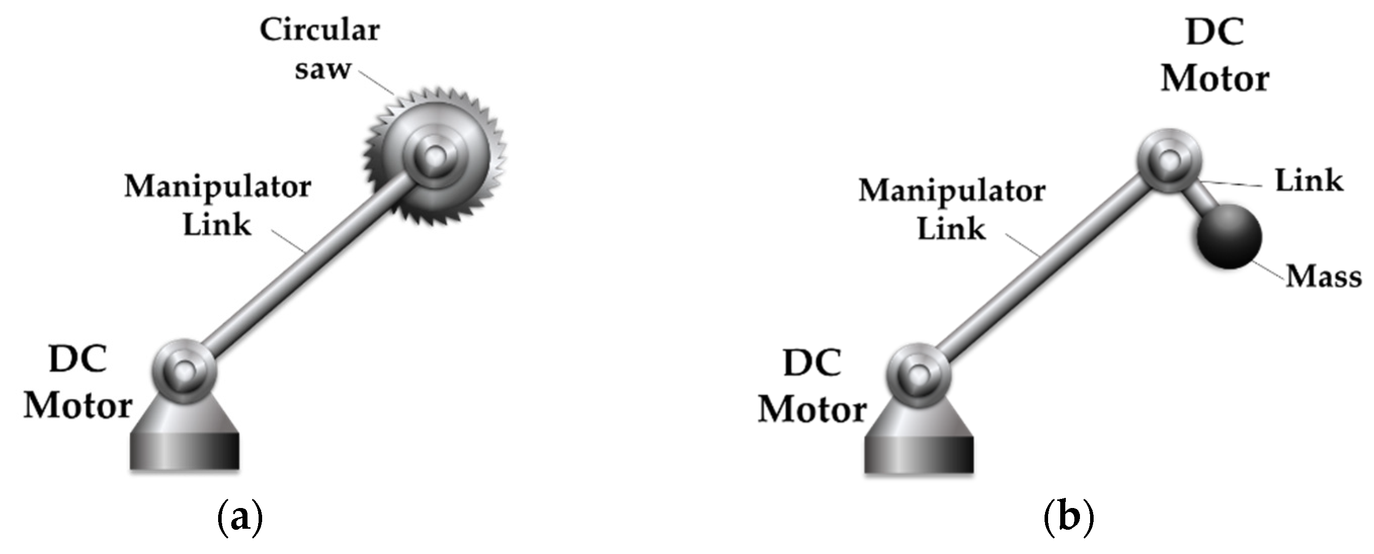
Figure 1 shows an example of a robotic manipulator with a non-ideal source of excitation, which will be considered in this work, represented by the use of a cutting tool attached to the end of the manipulator’s link.

Figure 1a shows a robotic manipulator with a link and a cutting tool at its end, representing a robotic system with a non-linear excitation source.

In Figure 1b we can see a representation of Figure 1a, in which the excitation source is composed of a DC motor and an unbalanced mass coupled to the motor shaft. For numerical simulations, the unbalanced mass will be considered as the second link of the robotic manipulator in rotational motion.

Considering Figure 1, this paper aims to contribute to the body of knowledge regarding the positioning control and dynamic behavior of a robotic manipulator with two degrees of freedom driven by DC electric motors, considering flexible joints and a non-ideal excitation source. As its main contribution, the paper presents the problem of controlling a manipulator submitted to a nonlinear excitation, investigating, through numerical simulations, the behavior of three different control strategies, including the feedforward control and the optimized PD control. The formulation of the feedforward control is demonstrated and the effectiveness of the proposed controls is presented by the analysis of the errors through the integral of the absolute magnitude of the error (IAE). This paper is organized as follows: Section 2 introduces the mathematical model used. In Section 3, the control design is described. In Section 4, numerical simulations are detailed considering the position control of the two links at fixed points (Case 1), and the control of the first link at a fixed point and the second in rotational movement, simulating the nonideal excitation source (Case 2). In Section 5 the percentage of positioning error reduction, and the integral of the absolute magnitude of the error (IAE) are presented, for the three proposed controls. Finally, the article is completed in Section 6.

2. Mathematical Model

Aiming to model the robotic manipulator as close as possible to the real physical model, the flexibility or elasticity of the material present in the structure of the materials was considered in the modeling, parameters that are often disregarded [26,27].

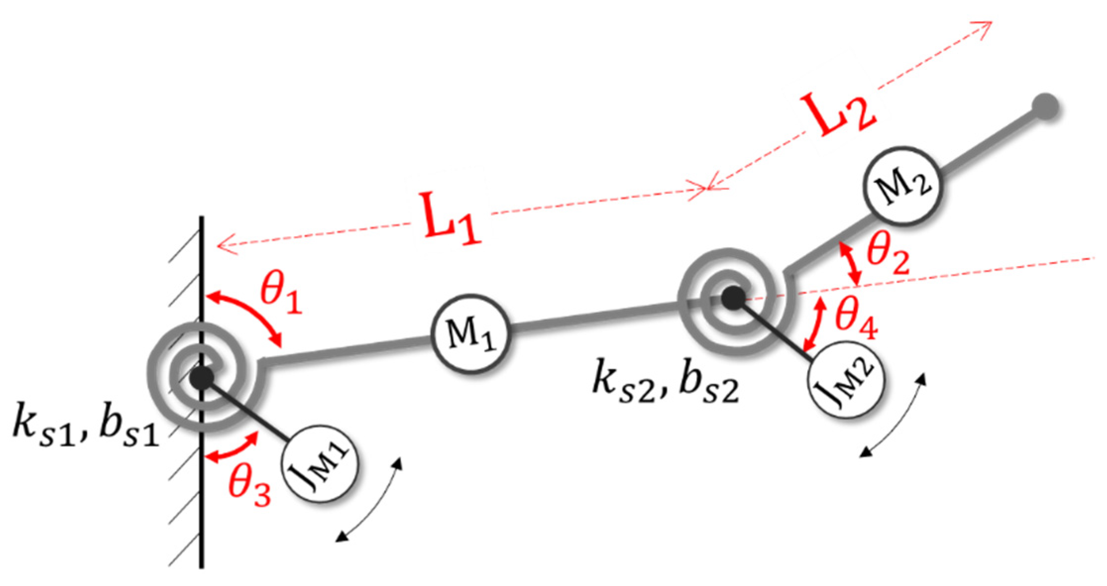
The schematic diagram shown in Figure 2 demonstrates the transmission with flexible joints between the DC motor and the links of a manipulator with 2 DOF.

Where ${\theta }_1$ represents the angle of the first link, ${\theta }_2$ represents the angle of the second link, ${\theta }_3$ is the shaft angle of the first motor, ${\theta }_4$ is the shaft angle of the second motor, $L_1$ is the length of the first link, $L_2$ is the length of the second link, $M_1$ is the mass of the first link, $M_2$ is the mass of the second link, $b_{s1}$ is the first joint damping factor, $b_{s2}$ is the second joint damping factor, $k_{s1}$ is the first joint spring factor, $k_{s2}$ is the second joint spring factor, $J_{M1}$ is the moment of inertia of the first rotor, and $J_{M2}$ is the moment of inertia of the second rotor.

For analysis and simulation, the modeling of a 2 DOF system with flexible joints was considered. Taking into account the generalized coordinates of Figure 2 described by the equations [19,22,24]:

$$\begin{array}{c}{p}_{x_1}=L_1\sin ({\theta }_1)\\ p_{y_1}=L_1\cos ({\theta }_2)\\ p_{x_2}=L_1\sin ({\theta }_1)+L_2\sin ({\theta }_1+{\theta }_2)\\ p_{y_2}=L_1\cos ({\theta }_2)+L_2\cos ({\theta }_1+{\theta }_2)\end{array}$$

(1)

The equation that defines the kinetic energy of the system represented by Figure 2 is given by [22,24]:

$${\xi }_c=\frac{1}{2}\left(M_1{\dot{p}}_{x_1}^2+M_1{\dot{p}}_{y_1}^2+M_2{\dot{p}}_{x_2}^2+M_2{\dot{p}}_{y_2}^2\right)$$

(2)

The potential energy can be obtained through the equation [22,24]:

$${\xi }_p=M_{1}g{L}_1\cos ({\theta }_1)+M_{2}g(L_1\cos ({\theta }_1)+L_2\cos ({\theta }_1+{\theta }_2))$$

(3)

From the energy balance we have the Lagrange equation [22,24]:

$$\xi ={\xi }_c-{\xi }_p$$

(4)

Substituting Equations (2) and (3) in Equation (4) we have [22,24]:

$$\begin{array}{l}\xi =\left(\frac{1}{2}{M}_1{L}_1^2+\frac{1}{2}{M}_2{L}_2^2+M_2{L}_{1}L2\cos ({\theta }_2)\right){\dot{\theta }}_1^2+\left(M_2{L}_2^2+M_2{L}_1{L}_2\cos ({\theta }_2)\right){\dot{\theta }}_2{\dot{\theta }}_1\cdots \hfill \\ \cdots +\frac{1}{2}{M}_2{L}_2^2{\dot{\theta }}_2^2-M_{2}g{L}_2\cos ({\theta }_1)-M_{2}g{L}_2\cos ({\theta }_1+{\theta }_2)-M_{1}g{L}_1\cos ({\theta }_1)\hfill \end{array}$$

(5)

To obtain the mathematical model, the Euler-Lagrange equation was considered [24]:

$$\frac{d}{dt}\left(\frac{\partial \xi }{\partial {\dot{\theta }}_i}\right)-\frac{\partial \xi }{\partial {\theta }_i}={\tau }_i$$

(6)

in which ${\theta }_i$ is the generalized coordinates, and ${\tau }_i$ is the torque. The torque equation is given by [24]:

$$\begin{array}{l}{\tau }_1=\left(M_2{L}_2^2+2M_2{L}_{1}L2\cos ({\theta }_2)+M_1{L}_1^2+M_2{L}_1^2\right)\ddot{\theta }+\left(M_2{L}_2^2+M_2{L}_1{L}_2\cos ({\theta }_2)\right){\ddot{\theta }}_2\cdots \hfill \\ \cdots -M_2{L}_2{L}_1\sin ({\theta }_2){\ddot{\theta }}_2-2M_2{L}_{1}L2\sin ({\theta }_2){\dot{\theta }}_1{\dot{\theta }}_2-M_{1}g{L}_1\sin ({\theta }_1)-M_{2}g{L}_1\sin ({\theta }_1)\cdots \hfill \\ \cdots -M_{2}g{L}_2\sin ({\theta }_1+{\theta }_2)-M_2{L}_2{L}_1\sin ({\theta }_2)\hfill \\ {\tau }_2=\left(M_2{L}_2^2+M_2{L}_1{L}_2\cos ({\theta }_2)\right){\ddot{\theta }}_1+M_2{L}_2^2{\ddot{\theta }}_2+M_2{L}_2^2{\ddot{\theta }}_2+M_2{L}_2{L}_1\sin ({\theta }_2){\dot{\theta }}_1^2\cdots \hfill \\ -M_{2}Lg{L}_2\sin ({\theta }_1+{\theta }_2)\hfill \end{array}$$

(7)

Adding the Friction Matrix $F(\dot{\theta })=\left[\begin{array}{cc}{\dot{\theta }}_1& {\dot{\theta }}_2\end{array}\right]$ in the system of Equation (7) and organizing it in matrix form, we have the system [22,24]:

$$\ddot{\theta }=M{(\theta )}^{-1}\left(-C(\theta ,\dot{\theta })\dot{\theta }-F(\dot{\theta })-G(\theta )+\mathsf{\tau }\right)$$

(8)

where $C(\theta ,\dot{\theta })=\left[\begin{array}{cc}{c}_1& 0\\ 0& c_2\end{array}\right]$, $F(\dot{\theta })=\left[\begin{array}{c}{\dot{\theta }}_1\\ {\dot{\theta }}_2\end{array}\right]$, $G(\theta ,\dot{\theta })=\left[\begin{array}{c}{g}_1\\ g_2\end{array}\right]$, and $M{(\theta )}^{-1}=\left[\begin{array}{cc}{p}_{11}& p_{12}\\ p_{21}& p_{22}\end{array}\right]$.

The constant $k_a$ represents the coefficient of the friction of the manipulator, while the coefficients of the matrices $C(\theta ,\dot{\theta })$ e $G(\theta ,\dot{\theta })$ can be determined by [22,24]:

$$\begin{array}{l}{c}_1=-M_2{L}_1{L}_2\mathrm{sen}({\theta }_2){\dot{\theta }}_2\\ c_2=-2M_2{L}_1{L}_2\mathrm{sen}({\theta }_2)(2{\dot{\theta }}_1+{\dot{\theta }}_2)\\ g_1=-(M_1+M_2)g{L}_1\mathrm{sen}({\theta }_1)-M_{2}g{L}_2\mathrm{sen}({\theta }_1+{\theta }_3)\\ g_2=-2M_2{L}_1{L}_2\mathrm{sen}({\theta }_2)(2{\dot{\theta }}_1+{\dot{\theta }}_2)\end{array}$$

(9)

The variables that represent joints with elastic characteristics ${\mathsf{\tau }}_s$ are given by [22,24]:

$${\mathsf{\tau }}_s=\left(\begin{array}{c}{b}_s({\dot{\theta }}_{M_1}-{\dot{\theta }}_1)+k_s({\theta }_{M_1}-{\theta }_1)\\ b_s({\dot{\theta }}_{M_2}-{\dot{\theta }}_2)+k_s({\theta }_{M_2}-{\theta }_2)\end{array}\right)$$

(10)

The equation that represents the DC motor corresponds to [20,22,24]:

$${\ddot{\mathsf{\theta }}}_M=\frac{1}{J_M}\left(k_{M}i-b_v{\dot{\mathsf{\theta }}}_M-{\mathsf{\tau }}_s\right)$$

(11)

Considering Equations (7) and (11), the mathematical model of the robotic manipulator can be written in state space form:

$$\begin{array}{l}{\dot{x}}_1=x_2\\ {\dot{x}}_2=-p_{11}{k}_s{x}_1+\alpha x_2-p_{12}{k}_s{x}_3+\beta x_4+p_{11}{k}_s{x}_5+p_{11}{b}_s{x}_6+p_{12}{k}_s{x}_7+p_{12}{b}_s{x}_8-p_{11}{g}_1-p_{12}{g}_2\\ {\dot{x}}_3=x_4\\ {\dot{x}}_4=-p_{21}{k}_s{x}_1+\gamma x_2-p_{22}{k}_s{x}_3+\delta x_4+p_{21}{k}_s{x}_5+p_{21}{b}_s{x}_6+p_{22}{k}_s{x}_7+p_{22}{b}_s{x}_8-p_{21}{g}_1-p_{22}{g}_2\\ {\dot{x}}_5=x_6\\ {\dot{x}}_6=\frac{1}{J_m}\left(-k_s{x}_1+b_s{x}_2-k_s{x}_5-\left(b_v+b_s\right)x_6+k_t{i}_1\right)\\ {\dot{x}}_7=x_8\\ {\dot{x}}_8=\frac{1}{J_m}\left(-k_s{x}_3+b_s{x}_4-k_s{x}_7-\left(b_v+b_s\right)x_8+k_t{i}_2\right)\end{array}$$

(12)

where $x_1={\theta }_1$, $x_2={\dot{\theta }}_1$, $x_3={\theta }_2$, $x_4={\dot{\theta }}_2$, $x_5={\theta }_{M_1}$, $x_6={\dot{\theta }}_{M_1}$, $x_7={\theta }_{M_2}$, $x_8={\dot{\theta }}_{M_2}$, $\alpha =-p_{11}(k_a+b_s)-p_{12}{c}_2$, $\beta =p_{11}{c}_1-p_{12}(k_a+b_s)$, $\gamma =-p_{21}(k_a+b_s)-p_{22}{c}_2$, $\delta =-p_{22}(k_a+b_s)-p_{21}{c}_1$, $p_{11}=\frac{-m_{22}}{-m_{12}{m}_{21}+m_{11}{m}_{22}}$, $p_{12}=\frac{-m_{21}}{-m_{12}{m}_{21}+m_{11}{m}_{22}}$, $p_{21}=\frac{-m_{12}}{-m_{12}{m}_{21}+m_{11}{m}_{22}}$, and $p_{22}=\frac{-m_{11}}{-m_{12}{m}_{21}+m_{11}{m}_{22}}$.

3. Proposed Control Law

The positioning control of the motor connections and the motor shaft is given by the electric current (i). Introducing the control of the electric current in the System (12), we will have the following system:

$$\begin{array}{l}{\dot{x}}_1=x_2\\ {\dot{x}}_2=-p_{11}{k}_s{x}_1+\alpha x_2-p_{12}{k}_s{x}_3+\beta x_4+p_{11}{k}_s{x}_5+p_{11}{b}_s{x}_6+p_{12}{k}_s{x}_7+p_{12}{b}_s{x}_8-p_{11}{g}_1-p_{12}{g}_2\\ {\dot{x}}_3=x_4\\ {\dot{x}}_4=-p_{21}{k}_s{x}_1+\gamma x_2-p_{22}{k}_s{x}_3+\delta x_4+p_{21}{k}_s{x}_5+p_{21}{b}_s{x}_6+p_{22}{k}_s{x}_7+p_{22}{b}_s{x}_8-p_{21}{g}_1-p_{22}{g}_2\\ {\dot{x}}_5=x_6\\ {\dot{x}}_6=\frac{1}{J}\left(-k_s{x}_1+b_s{x}_2-k_s{x}_5-\left(b_v+b_s\right)x_6+k_t{U}_1\right)\\ {\dot{x}}_7=x_8\\ {\dot{x}}_8=\frac{1}{J}\left(-k_s{x}_3+b_s{x}_4-k_s{x}_7-\left(b_v+b_s\right)x_8+k_t{U}_2\right)\end{array}$$

(13)

where $U_i=u_i+{\tilde{u}}_i$, $u_i$ is the state feedback control, and ${\tilde{u}}_i$ is the feedforward control, the latter being composed of terms that depend on the gravitational force g in the following form [15]:

$$\begin{array}{l}{\tilde{u}}_1=p_{11}{g}_1+p_{12}{g}_2\\ {\tilde{u}}_2=p_{21}{g}_1+p_{22}{g}_2\end{array}$$

(14)

In this paper, the state feedback control can be a PD control or a PID control. The gains of control given by: $K_p$ is the proportional gain, $K_d$ is the derived gain, and $K_i$ is the corresponding integral gain of the control loop, respectively.

The errors are $e_1={\tilde{x}}_1-x_1$, $e_2={\dot{\tilde{x}}}_1-{\dot{x}}_1$, $e_3={\tilde{x}}_3-x_3$, $e_4={\dot{\tilde{x}}}_3-{\dot{x}}_3$, $e_5={\tilde{x}}_5-x_5$, $e_6={\dot{\tilde{x}}}_5-{\dot{x}}_5$, $e_7={\tilde{x}}_7-x_7$ and $e_8={\dot{\tilde{x}}}_7-{\dot{x}}_7$, where ${\tilde{x}}_{-}$ represent the desired states for the angular position of the links and the motor shaft.

The LQR control was used to determine the gains of $K_p$ e $K_d$, which allows the design of an optimal PD control.

$$K=R^{-1}{B}^{\mathrm{T}}P$$

(15)

where $K_p=k_{i,j}$ for $j=1,3,5,7\dots$, $K_d=k_{i,j}$ for $j=2,4,6,8\dots$, and for a PD control: $U_i$. The matrix $P$ is obtained by solving the following Riccati equation:

$$A^{T}P+PA-PB{R}^{-1}{B}^{T}P+Q=0$$

(16)

The cost function for the control problem for optimal PD control is given by:

$$J=\frac{1}{2}{\displaystyle \underset{t_0}{\overset{\infty }{\int }}(e^{T}Qe+u^{T}Ru)}dt$$

(17)

where $Q$ and $R$ are positive definite matrices.

4. Numerical Simulation

The proposed control technique has been simulated in MATLAB software (license: MathWorks 1115175), considering the “ode45” integrator, with fixed-step integration (h = 0.10). Numerical simulations considered two different cases for the efficiency analysis of the proposed control. In the first case, the links were positioned at two fixed points. In the second case, the first link was positioned at a fixed point, while the second link was in kept rotational motion, representing an engine with unbalanced mass (non-ideal system).

The parameters used in numerical simulations are shown in

Table 1. Parameters used in simulations.

Parameter	Value	Parameter	Value
M1	1 [$\mathrm{kg}$]	ks	450 [$\mathrm{Nm}/\mathrm{rad}$]
M2	1 [$\mathrm{kg}$]	bs	510 [$\mathrm{Nms}/\mathrm{rad}$]
L1	0.8 [$\mathrm{m}$]	ka	6 [$\mathrm{Nm}/\mathrm{rad}$]
L2	0.8 [$\mathrm{m}$]	bv	0.02 [$\mathrm{Nms}/\mathrm{rad}$]
g	9.8 [$\mathrm{m}/{\mathrm{s}}^2$]	J	0.0002$\left[{\mathrm{kgm}}^2\right]$
kt	0.8$\left[\mathrm{Nm}/\mathrm{A}\right]$	xi(0), i = 1:8	0

:

Considering the parameters in Table 1 and Equation (13) in matrix form $\dot{X}=AX+BU$, we have the following matrices A and B:

$$A=\left[\begin{array}{cccccccc}1& 0& 0& 0& 0& 0& 0& 0\\ -k{p}_{11}& \alpha & -k{p}_{12}& \beta & k{p}_{11}& b_s{p}_{11}& k{p}_{12}& b_s{p}_{12}\\ 0& 0& 1& 0& 0& 0& 0& 0\\ -k{p}_{21}& \gamma & -k{p}_{22}& \delta & k{p}_{21}& b_s{p}_{21}& k{p}_{22}& b_s{p}_{22}\\ 0& 0& 0& 0& 0& 1& 0& 0\\ \frac{-k}{J}& \frac{b_s}{J}& 0& 0& \frac{-k}{J}& \frac{-\left(b_s+b_v\right)}{J}& 0& 0\\ 0& 0& 0& 0& 0& 0& 1& 0\\ 0& 0& \frac{-k}{J}& \frac{b_s}{J}& 0& 0& \frac{-k}{J}& \frac{-\left(b_s+b_v\right)}{J}\end{array}\right]\mathrm{and}B=\left[\begin{array}{cc}0& 0\\ 0& 0\\ 0& 0\\ 0& 0\\ 0& 0\\ \frac{k_t}{J}& 0\\ 0& 0\\ 0& \frac{k_t}{J}\end{array}\right]$$

Defining the matrices Q and R:

$$Q=\left[\begin{array}{cccccccc}{10}^9& 0& 0& 0& 0& 0& 0& 0\\ 0& {10}^2& 0& 0& 0& 0& 0& 0\\ 0& 0& {10}^9& 0& 0& 0& 0& 0\\ 0& 0& 0& {10}^2& 0& 0& 0& 0\\ 0& 0& 0& 0& {10}^9& 0& 0& 0\\ 0& 0& 0& 0& 0& {10}^2& 0& 0\\ 0& 0& 0& 0& 0& 0& {10}^9& 0\\ 0& 0& 0& 0& 0& 0& 0& {10}^2\end{array}\right]\mathrm{and}R=\left[\begin{array}{cc}{10}^{-3}& 0\\ 0& {10}^{-3}\end{array}\right]$$

Considering Equation (15), we obtain the optimal PD gains:

$$K=\left[\begin{array}{cccccccc}-708316& -5234.9& 989.1866& 1928.63& -705899.35& 74.66& -1086.83& 0.15\\ 1036.83& 1928.9& -707146.8& -3008.18& -989.18& 0.150& -707630.3& 74.84\end{array}\right]$$

(18)

The gains of integrative control are given by and considered: for $u_1$($K_{i_1}=2179449.33$, $K_{i_3}=224821.58$, $K_{i_5}=2280104.28$, and $K_{i_7}=21848.79$) and for $u_2$($K_{i_1}=162457.09$, $K_{i_3}=2950790.59$, $K_{i_5}=170105.19$, and $K_{i_7}=300778.54$) [3].

4.1. Control Design for the First Case: Two Links Positioned at Two Fixed Points

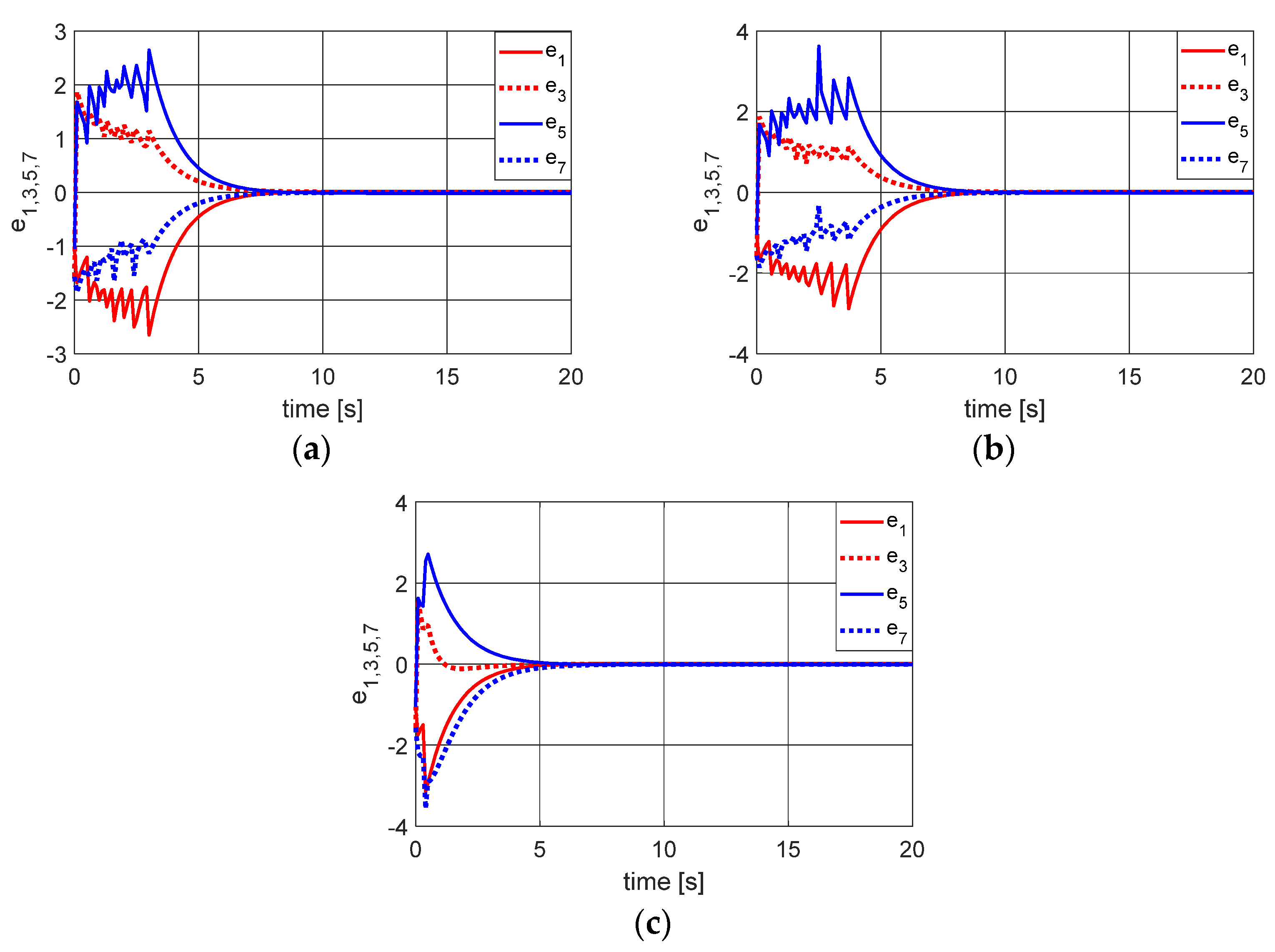
Considering the positioning of the two links at fixed points, the desired points in this work were defined at ${\tilde{x}}_1={\tilde{x}}_5=\frac{\pi }{3}$, ${\tilde{x}}_3={\tilde{x}}_7=\frac{\pi }{2}$, and ${\tilde{x}}_2={\tilde{x}}_4={\tilde{x}}_6={\tilde{x}}_8=0$, while the errors were given by $e_1={\tilde{x}}_1-x_1$ [rad], $e_2={\dot{\tilde{x}}}_1-{\dot{x}}_1$ [rad/s], $e_3={\tilde{x}}_3-x_3$ [rad], $e_4={\dot{\tilde{x}}}_3-{\dot{x}}_3$ [rad/s], $e_5={\tilde{x}}_5-x_5$ [rad], $e_6={\dot{\tilde{x}}}_5-{\dot{x}}_5$ [rad/s], $e_7={\tilde{x}}_7-x_7$ [rad], and $e_8={\dot{\tilde{x}}}_7-{\dot{x}}_7$ [rad/s].

Figure 3 shows the variations of positioning errors for two fixed points.

Table 2. Positioning error for point-to-point position control.

Error	PD	PD + Feedforward	PDI+ Feedforward
$e_1$	0.02022	0.0202	0.01989
$e_3$	0.005444	0.005422	0.000777
$e_5$	−0.01863	−0.01861	−0.01802
$e_7$	−0.002884	−0.002804	−0.00162

shows the highest error value for t = [15:20] seconds for Figure 3.

As we can see in Figure 3, and in the data in Table 2, the three control strategies proved efficient, emphasizing that the PD controller was enough to produce results very close to those of the PD + feedforward controller. As the PD control was obtained from the LQR, its response is an optimal PD control, which justifies its performance. Similar behavior was also observed in [5].

4.2. Control Design for the Second Case: One Link Positioned at a Fixed Point and the Other in Rotational Motion

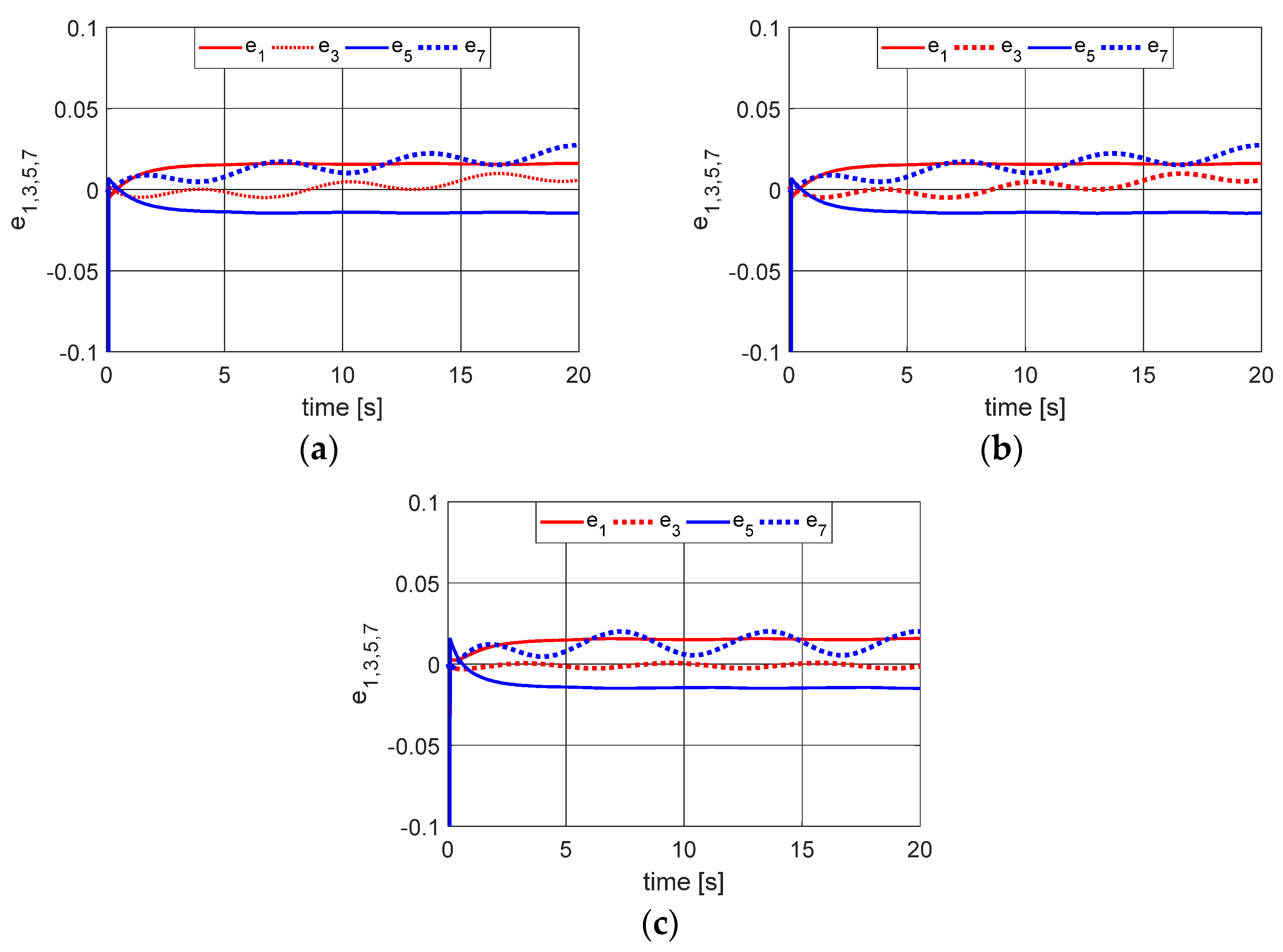
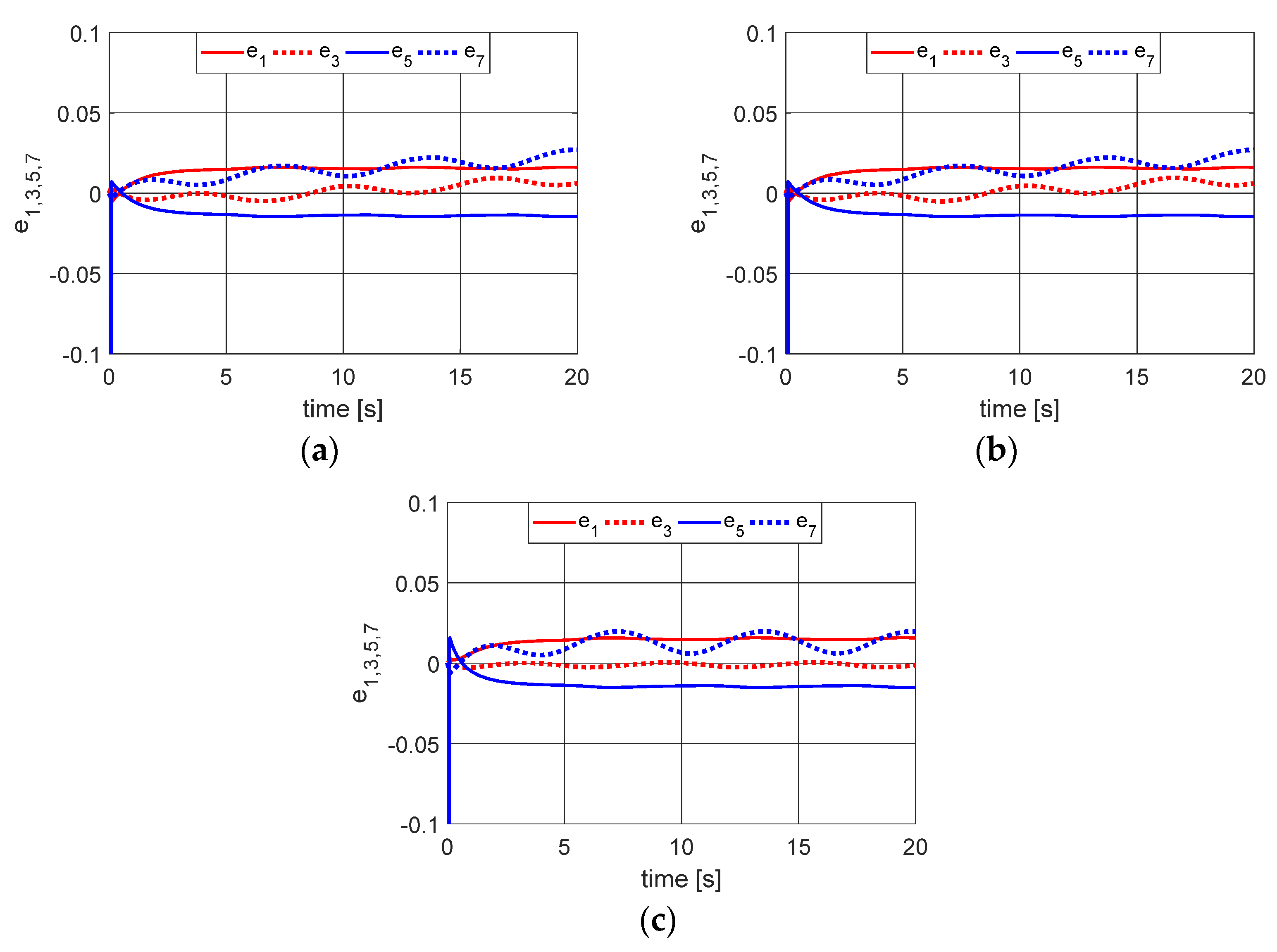
Considering the case in which the second link represents a rotational mechanism, thus generating a non-ideal excitation source, the desired points were defined as: ${\tilde{x}}_1={\tilde{x}}_5=\frac{\pi }{3}$, ${\tilde{x}}_3={\tilde{x}}_7=\sin (t)+t$, ${\tilde{x}}_2={\tilde{x}}_6=0$, and ${\tilde{x}}_4={\tilde{x}}_8=\cos (t)+1$.

Figure 4 shows the position error variations considering the case of $M_2=1$ [kg] and $L_2=0.05$ [m].

Table 3. Positioning error for position control in the case of one link at a fixed point and the other in rotational motion.

Error	PD	PD + Feedforward	PDI+ Feedforward
$e_1$	0.01611	0.01609	0.0158
$e_3$	0.009913	0.005553	−0.002616
$e_5$	−0.01453	−0.01452	−0.01408
$e_7$	0.02739	0.02735	0.0201

shows the highest error value for t = [15:20] seconds for Figure 4.

Analyzing the results presented in Figure 4 and the data in Table 3, we can observe an increase in the error, which was expected, taking into account that the second link will be in rotational movement. As the rotation movement of the second link interferes with the positioning of the first link, the behavior of the system is classified as non-ideal, which makes it difficult to control with the same precision observed in the case of a fixed point.

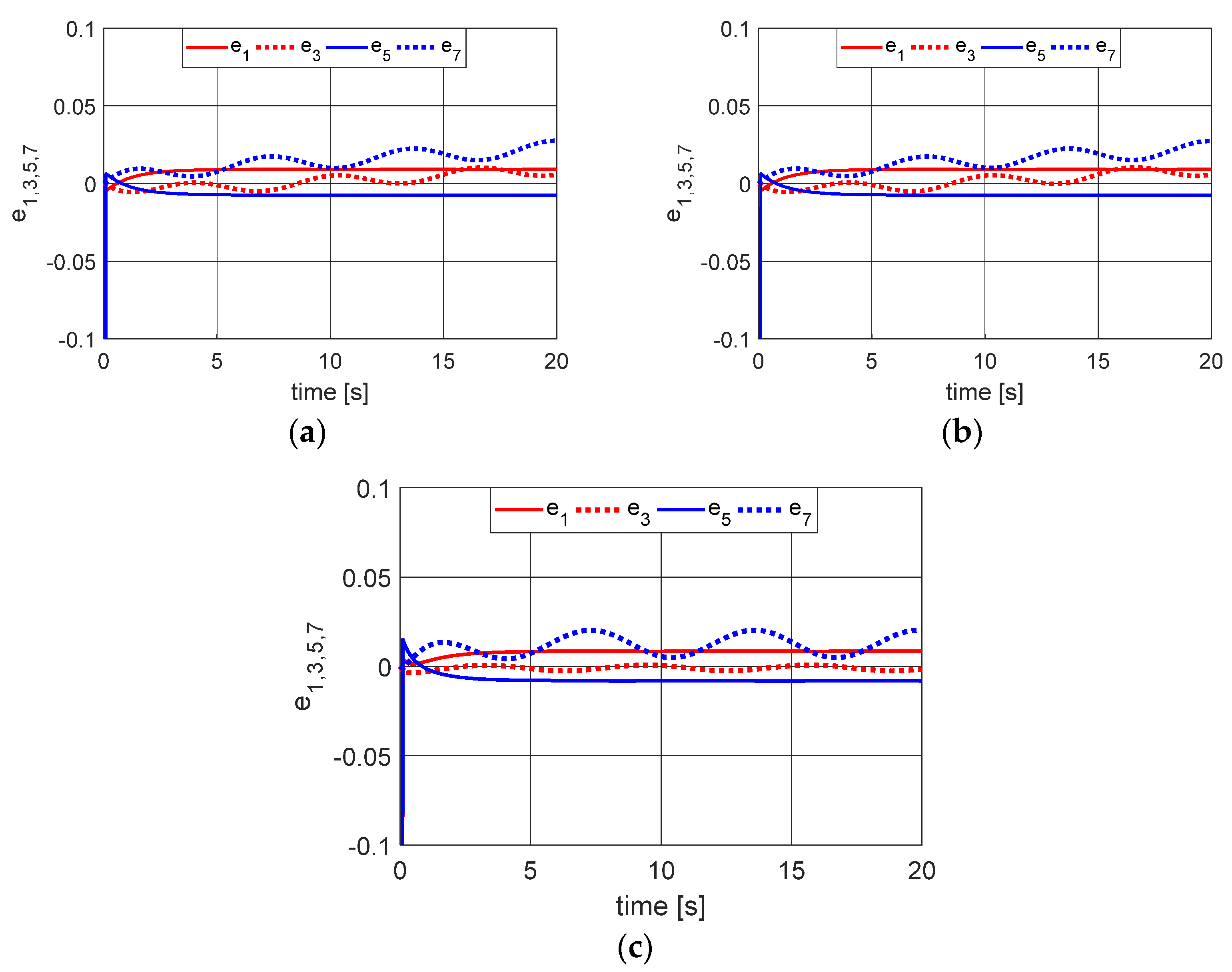
Figure 5 shows the position error variations considering the case of $M_2=1$ [kg] and $L_2=0.1$ [m].

Table 4. Positioning error for position control on a fixed point and the other in rotational motion.

Error	PD	PD + Feedforward	PDI+ Feedforward
$e_1$	0.01621	0.01619	0.01575
$e_3$	0.009697	0.009421	−0.002373
$e_5$	−0.01469	−0.01463	−0.01403
$e_7$	0.02715	0.02699	0.01977

shows the highest error value for t = [15:20] seconds for Figure 5.

The results shown in Figure 5 and Table 4 indicated that the increase in the length of Link 2 did not significantly interfere with the efficiency of the presented controls. These results demonstrated that the control does not lose efficiency for small variations in the length of the second link.

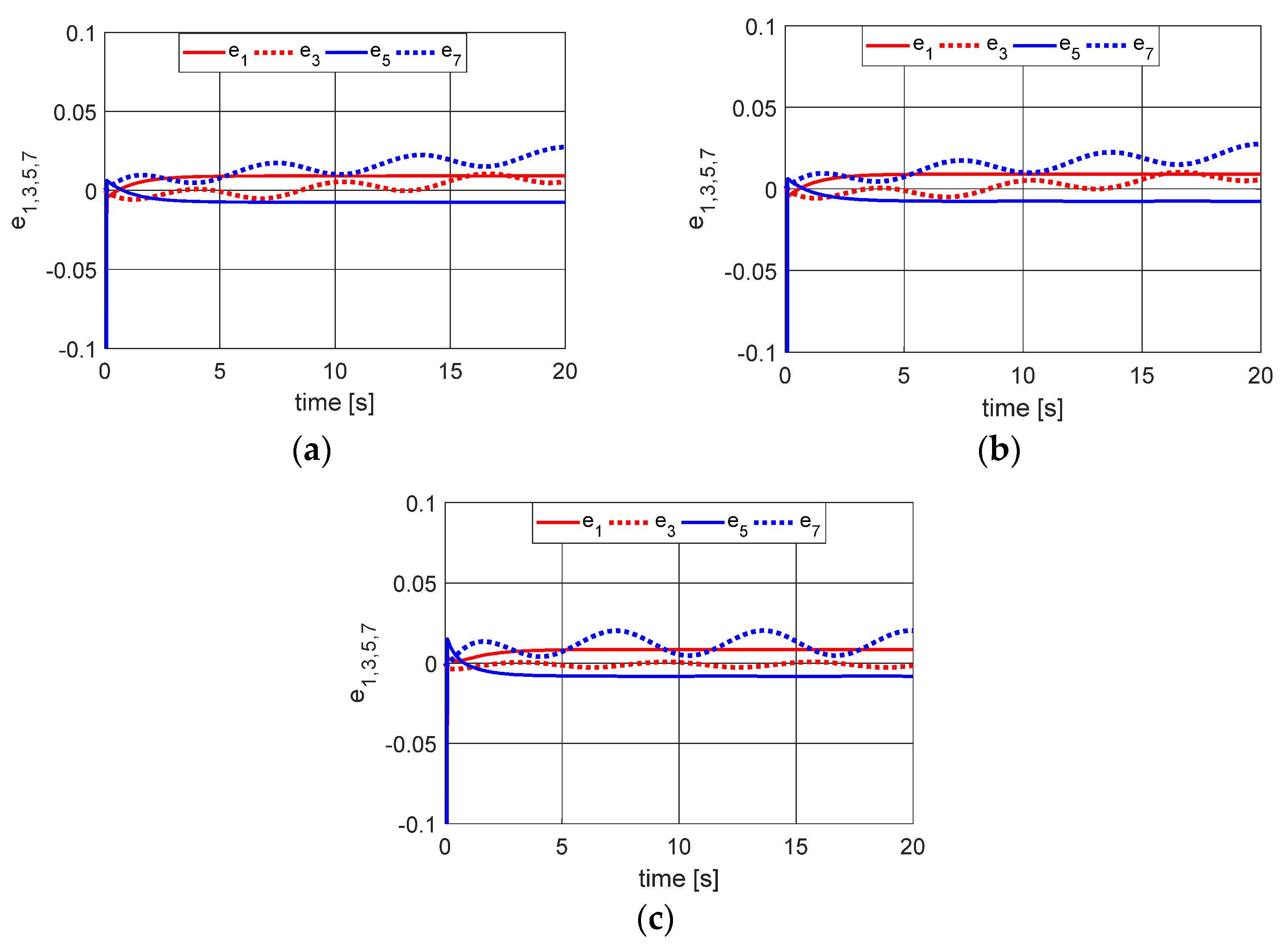
Figure 6 shows the position error variations considering the case of $M_2=0.1$ [kg] and $L_2=0.1$ [m].

Table 5. Positioning error for position control on a fixed point and the other in rotational motion.

Error	PD	PD + Feedforward	PDI+ Feedforward
$e_1$	0.009178	0.009169	0.0085555
$e_3$	0.01041	0.01031	−0.002513
$e_5$	−0.007585	−0.007575	−0.007162
$e_7$	0.02742	0.02735	0.02022

shows the highest error value for t = [15:20] seconds for Figure 6.

The results presented in Figure 6 and Table 5 show that the reduction of the mass $M_2$ did not influence the result of the PD control and PD + feedforward controls; however, we can observe that the PD + feedforward control had reduced errors compared to that observed for the mass $M_2$ higher. The result indicates that $M_2$ influences the efficiency of the PID control.

Figure 7 shows the position error variations considering the case of $M_2=0.05$ [kg] and $L_2=0.1$ [m].

Table 6. Positioning error for position control on a fixed point and the other in rotational motion.

Error	PD	PD + Feedforward	PDI+ Feedforward
$e_1$	0.009184	0.009178	0.008543
$e_3$	0.01031	0.01028	0.001494
$e_5$	−0.007565	−0.007561	−0.007164
$e_7$	0.02743	0.02740	0.02023

shows the highest error value for t = [15:20] seconds for Figure 7.

The results shown in Figure 7 and Table 6 confirm that $m_2$ influences the efficiency of the PID control.

5. Discussion

Table 7. Percentage of positioning error reduction concerning PD + feedforward control (PD_f) and PID + feedforward control (PID_f) for position control on a fixed point and the other in rotational motion.

	L2 = 0.05 [m] M2 = 1 [kg]		L2 =0.10 [m] M2= 1 [kg]		L2 = 0.10 [m] M2 = 0.1 [kg]		L2 = 0.05 [m] M2 = 0.1 [kg]
Error	PD	PID	PD	PID	PD	PID	PD	PID
$e_1$	0.12%	0.01%	0.12%	0.02%	0.09%	0.06%	0.06%	0.06%
$e_3$	0.43%	0.73%	2.84%	0.75%	0.96%	0.75%	0.29%	0.85%
$e_5$	0.06%	0.03%	0.40%	0.04%	0.13%	0.05%	0.05%	0.05%
$e_7$	0.14%	0.26%	0.58%	0.27%	0.25%	0.26%	0.10%	0.26%

presents the percentage of error reduction considering the feedforward control plus the PD control and with the PID control with feedforward control for position control on a fixed point and the other in rotational motion.

Table 8. The integral of the absolute magnitude of the error (IAE) concerning PD control, PD (PD_f), and PID control with feedforward control (PID_f) for position control on a fixed point and the other in rotational motion.

	L2 = 0.05 [m] M2 = 1 [kg]			L2 =0.10 [m] M2= 1 [kg]			L2 = 0.10 [m] M2 = 0.1 [kg]			L2 = 0.05 [m] M2 = 0.1 [kg]
IAE	PD	PDf	PIDf	PD	PDf	PIDf	PD	PDf	PIDf	PD	PDf	PIDf
$e_1$	0.289	0.289	0.389	0.291	0.292	0.239	0.288	0.289	0.234	0.234	0.288	0.234
$e_3$	0.367	0.367	0.378	0.363	0.363	0.374	0.242	0.242	0.257	0.257	0.243	0.257
$e_5$	0.075	0.075	0.025	0.072	0.073	0.024	0.079	0.080	0.026	0.026	0.080	0.026
$e_7$	0.398	0.397	0.389	0.394	0.393	0.385	0.273	0.272	0.260	0.261	0.273	0.261

shows the integral of the absolute magnitude of the error (IAE) considering the PD control (PD) and PD + feedforward control (PD_f) and obtained from the LQR control and PID + feedforward control (PID_f) for position control on a fixed point and the other in rotational motion.

Analyzing the results shown in Table 7, it can be seen that the control strategy with PID Control+ Feedforward Control is the strategy that obtained the best performance, a result consistent with what was expected, since the inclusion of the integrative control has as the main objective to reduce the error in the regime, and the inclusion of the feedforward control to eliminate the influence of gravitational force in the calculation of the feedback control. However, it should be noted that the positioning error of the first link ($e_1={\tilde{x}}_1-x_1$) is very similar for the three proposed strategies and that the control only with the PD control obtained results as efficiently as the others. This result can be explained due to the fact PD control was obtained using the LQR, which provided an optimal PD control. The results shown in Table 8 confirm the results obtained in Table 7.

Table 9. The integral of the absolute magnitude of the error (IAE) concerning PD control, PD (PD_f), and PID control with feedforward control (PID_f) for position control on a fixed point and the other in rotational motion.

IAE	PD	PDf	PIDf
$e_1$	5.252	5.790	5.906
$e_3$	8.672	10.680	4.244
$e_5$	5.143	5.724	1.134
$e_7$	8.897	10.741	4.514

shows the integral of the absolute magnitude of the error (IAE) considering the PD control (PD), PD + feedforward control (PD_f), and PID + feedforward control (PID_f) for position control on two fixed points. Similar behavior was also observed in [5].

Analyzing the integral of the absolute magnitude of the error (IAE) data, shown in Table 9, we can observe the contribution of the integrative term in the control. The results demonstrate that the PID + feedforward control was more efficient than the other two analyzed controls. We can also observe that the optimal PD control and the PD + feedforward control presented similar results, demonstrating the importance of designing optimal controllers. Similar behavior was also observed in [5].

6. Conclusions

The numerical results presented in this work show that we can consider a robotic arm with flexible joints as a system with non-ideal excitation sources. This behavior was clearer with a link in rotational movement, behavior similar to that observed when we coupled a motor to the end of the first link.

Analyzing the presented results, and considering the analysis of the influence of the rotational movement of the second link on the positioning of the first link (non-ideal source of excitation), it can be observed that there is a better error for smaller masses of m² and smaller length L₂, parameters of the second link. Furthermore, it should be noted that for all cases analyzed, the errors were centesimal, demonstrating that the proposal of an optimal PD control through the use of the LQR, made it possible to obtain an efficient control and that the inclusion of the integrative term and the feedforward control made it possible to reduce a little more this error, which is extremely important for positioning control with millimeter precision.

The numerical results also showed that the combination of PID control is the most suitable for cases in which the links are subject to rotational movement (vibration) and that the PD and LQR control demonstrates efficiency when combined with the feed-forward gain.

References

1. Manzoor, S.; Islam, R.U.; Khalid, A.; Samad, A.; Iqbal, J. An open-source multi-DOF articulated robotic educational platform for autonomous object manipulation. Robot. Comput. -Integr. Manuf. 2014, 30, 351–362. [Google Scholar] [CrossRef]
2. Siciliano, B.; Khatib, O. Springer Handbook of Robotics; Springer: Berlin/Heidelberg, Germany, 2016. [Google Scholar]
3. Kumar, J.; Kumar, V.; Rana, K.P.S. Fractional-order self-tuned fuzzy PID controller for three-link robotic manipulator system. Neural Comput. Appl. 2020, 32, 7235–7257. [Google Scholar] [CrossRef]
4. Lu, P.; Wenkai, H.; Xiao, J.; Zhou, F.; Hu, W. Adaptive Proportional Integral Robust Control of an Uncertain Robotic Manipulator Based on Deep Deterministic Policy Gradient. Mathematics 2021, 9, 2055. [Google Scholar] [CrossRef]
5. Saleem, O.; Abbas, F.; Iqbal, J. Complex Fractional-Order LQIR for Inverted-Pendulum-Type Robotic Mechanisms: Design and Experimental Validation. Mathematics 2023, 11, 913. [Google Scholar] [CrossRef]
6. Ali, K.; Mehmood, A.; Muhammad, I.; Razzaq, S.; Iqbal, J. Control of an Anthropomorphic Manipulator using LuGre Friction Model-Design and Experimental Validation. J. Mech. Eng. 2021, 67, 401–410. [Google Scholar] [CrossRef]
7. Ali, K.; Ullah, S.; Mehmood, A.; Mostafa, H.; Marey, M.; Iqbal, J. Adaptive FIT-SMC Approach for an Anthropomorphic Manipulator with Robust Exact Differentiator and Neural Network-Based Friction Compensation. IEEE Access 2022, 10, 3378–3389. [Google Scholar] [CrossRef]
8. Asghar, A.; Iqbal, M.; Khaliq, A.; Rehman, S.; Iqbal, J. Performance comparison of structured H ∞ based looptune and LQR for a 4-DOF robotic manipulator. PLoS ONE 2022, 17, e0266728. [Google Scholar] [CrossRef] [PubMed]
9. Rezoug, A.; Iqbal, J.; Tadjine, M. Extended grey wolf optimization–based adaptive fast nonsingular terminal sliding mode control of a robotic manipulator. Proc. Inst. Mech. Eng. Part I J. Syst. Control. Eng. 2022, 236, 1738–1754. [Google Scholar] [CrossRef]
10. Tusset, A.M.; De Lima, J.J.; Janzen, F.C.; Paula Filho, P.L.; Luz Junior, J.A.G.; Balthazar, J.M.; Kossoski, A. A Hybrid PID-LQR Control Applied in Positioning Control of Robotic Manipulators Subject to Excitation from Non-ideal Sources. In Mechanisms and Machine Science, 1st ed.; Springer: Cham, Switzerland, 2022; Volume 116, pp. 393–403. [Google Scholar] [CrossRef]
11. Tusset, A.M.; Paula Filho, P.L.; Piccirillo, V.; Lenzi, G.G.; Balthazar, J.M.; Oliveira, C.; Varanis, M. Dynamic Analysis and PID Control of a Double Pendulum Arm Excited by a Nonideal Source. In Mechanisms and Machine Science, 1st ed.; Springer: Cham, Switzerland, 2022; Volume 116, pp. 343–356. [Google Scholar] [CrossRef]
12. Wang, Y.N.; Mai, T.L.; Mao, J.X. Adaptive motion/force control strategy for non-holonomic mobile manipulator robot using recurrent fuzzy wavelet neural networks. Eng. Appl. Artif. Intell. 2014, 34, 137–153. [Google Scholar] [CrossRef]
13. Zakia, U.; Moallem, M.; Menon, C. PID-SMC controller for a 2-DOF planar robot. In Proceedings of the 2019 International Conference on Electrical, Computer and Communication Engineering, Cox’sBazar, Bangladesh, 7–9 February 2019; pp. 1–5. [Google Scholar] [CrossRef]
14. Van, M.; Do, X.P.; Mavrovouniotis, M. Self-tuning fuzzy PID-nonsingular fast terminal sliding mode control for robust fault tolerant control of robot manipulators. ISA Trans. 2019, 1, 1–12. [Google Scholar] [CrossRef] [PubMed]
15. Rad, S.A.; Tamizi, M.G.; Mirfakhar, A.; Masouleh, M.T.; Kalhor, A. Control of a two-DOF parallel robot with unknown parameters using a novel robust adaptive approach. ISA Trans. 2021, 117, 70–84. [Google Scholar] [CrossRef]
16. Yang, S.; Han, J.; Xia, L.; Chen, Y.-H. An optimal fuzzy-theoretic setting of adaptive robust control design for a lower limb exoskeleton robot system. Mech. Syst. Signal Process. 2020, 141, 106706. [Google Scholar] [CrossRef]
17. Korayem, M.H.; Nekoo, S.R. Finite-time state-dependent Riccati equation for time-varying nonaffine systems: Rigid and flexible joint manipulator control. ISA Trans. 2015, 54, 125–144. [Google Scholar] [CrossRef] [PubMed]
18. Korayem, M.H.; Nekoo, S.R. State-dependent differential Riccati equation to track control of time-varying systems with state and control nonlinearities. ISA Trans. 2015, 57, 117–135. [Google Scholar] [CrossRef] [PubMed]
19. Korayem, M.H.; Irani, M.; Nekoo, S.R. Load maximization of flexible joint mechanical manipulator using nonlinear optimal controller. Acta Astronaut. 2011, 69, 458–469. [Google Scholar] [CrossRef]
20. Korayem, M.H.; Irani, M.; Nekoo, S.R. Analysis of manipulators using SDRE: A closed loop nonlinear optimal control approach. Scientia Iranica. Trans. B Mech. Eng. 2020, 17, 456–467. [Google Scholar]
21. Lima, J.J.; Tusset, A.M.; Janzen, F.C.; Piccirillo, V.; Nascimento, C.B.; Balthazar, J.M.; Brasil, R.M.L.R.F. Nonlinear state estimation and control applied to a manipulator robotic including drive motor. Math. Eng. Sci. Aerosp. 2014, 5, 413–425. [Google Scholar]
22. Lima, J.J.; Tusset, A.M.; Janzen, F.C.; Piccirillo, V.; Nascimento, C.B.; Balthazar, J.M.; Brasil, R.M.L.R.F. SDRE applied to position and vibration control of a robot manipulator with a flexible link. J. Theor. Appl. Mech. 2016, 54, 1067–1078. [Google Scholar] [CrossRef] [Green Version]
23. Lima, J.J.; Rocha, R.T.; Janzen, F.C.; Tusset, A.M.; Bassinello, D.G.; Balthazar, J.M. Position control of a manipulator robotic arm considering flexible joints driven by a DC motor and a controlled torque by a MR-brake. In Proceedings of the SME 2016 International Mechanical Engineering Congress and Exposition, Dynamics, Vibration, and Control, Phoenix, AZ, USA, 11–17 November 2016; Volume 4, p. V04BT05A022. [Google Scholar]
24. Lima, J.J.; Balthazar, J.M.; Rocha, R.T.; Janzen, F.C.; Bernardini, D.; Litak, G.; Bassinello, D.G.; Tusset, A.M. On positioning and vibration control application to robotic manipulators with a nonideal load carrying. Shock Vib. 2019, 2019, 5408519. [Google Scholar] [CrossRef]
25. Tusset, A.; Balthazar, J.; Felix, J. On elimination of chaotic behavior in a non-ideal portal frame structural system, using both passive and active controls. J. Vib. Control. 2012, 16, 803–813. [Google Scholar] [CrossRef]
26. Lewis, F.L.; Dawson, D.M.; Abdallah, C.T. Robot Manipulator Control: Theory and Practice; CRC Press: Boca Raton, FL, USA, 2003. [Google Scholar]
27. Jabłoński, R.; Turkowski, M.; Szewczyk, R. (Eds.) Recent Advances in Mechatronics; Springer: Berlin/Heidelberg, Germany, 2007. [Google Scholar] [CrossRef]
Figure 1. (a) Example of a robotic manipulator with a non-ideal excitation source. (b) Representation of the non-ideal system using a DC motor with an unbalanced mass.
Robotics 12 00051 g001
Figure 2. Schematic of the manipulator with flexible joints.
Robotics 12 00051 g002
Figure 3. Positioning error. (a) PD control. (b) PD + feedforward control. (c) PDI + feedforward control.
Robotics 12 00051 g003
Figure 4. Positioning error for the case of M 2 = 1 [kg] and L 2 = 0.05 [m]. (a) PD control. (b) PD + feedforward control. (c) PDI+ feedforward control.
Robotics 12 00051 g004
Figure 5. Positioning error for the case of M 2 = 1 [kg] and L 2 = 0.1 [m]. (a) PD control. (b) PD + feedforward control. (c) PDI+ feedforward control.
Robotics 12 00051 g005
Figure 6. Positioning error for the case of M 2 = 0.1 [kg] and L 2 = 0.1 [m]. (a) PD control. (b) PD + feedforward control. (c) PDI + feedforward control.
Robotics 12 00051 g006
Figure 7. Positioning error for the case of M 2 = 0.05 [kg] and L 2 = 0.1 [m]. (a) PD control. (b) PD + feedforward control. (c) PDI+ feedforward control.
Robotics 12 00051 g007