
Energy Efficiency of a Wheeled Bio-Inspired Hexapod Walking Robot in Sloping Terrain

Department of Intelligent Systems, Faculty of Information Technology, Brno University of Technology, Božetěchova 2, 612 66 Brno, Czech Republic
*
Author to whom correspondence should be addressed.
Robotics 2023, 12(2), 42; https://doi.org/10.3390/robotics12020042
Submission received: 7 February 2023
/
Revised: 10 March 2023
/
Accepted: 13 March 2023
/
Published: 15 March 2023
(This article belongs to the Topic Intelligent Systems and Robotics)
Abstract
:Multi-legged robots, such as hexapods, have great potential to navigate challenging terrain. However, their design and control are usually much more complex and energy-demanding compared to wheeled robots. This paper presents a wheeled six-legged robot with five degrees of freedom, that is able to move on a flat surface using wheels and switch to gait in rugged terrain, which reduces energy consumption. The novel joint configuration mimics the structure of insect limbs and allows our robot to overcome difficult terrain. The wheels reduce energy consumption when moving on flat terrain and the trochanter joint reduces energy consumption when moving on slopes, extending the operating time and range of the robot. The results of experiments on sloping terrain are presented. It was confirmed that the use of the trochanter joint can lead to a reduction in energy consumption when moving in sloping terrain.
1. Introduction
Legged robots are well suited to navigate rugged terrain. Although they are more complex to operate than wheeled or tracked robots, new walking robots of different shapes and sizes are being designed. As the number of limbs increases, the stability and number of gaits of the robot also increases. The greatest improvement is observed between four- and six-legged robots [1]. Walking robots can be statically or dynamically stable and can move by walking, running, jumping or climbing. The most common statically stable legged robots are hexapods. With six limbs, they can move using many different gaits. Many hexapods have only three degrees of freedom per limb, so they can only affect the position of foot tip; namely MAX [2], AMOS II [3], Messor-II [4], DLR-Crawler [5] or HECTOR [6]. However, four or more degrees of freedom per leg increases the number of possible robot stances. ASTERISK [7], or Lauron V [8], has four degrees of freedom per leg and Weaver, a proprioceptive-controlled hexapod, has five degrees of freedom per leg [9]. Besides the number of degrees of freedom of the limb, the arrangement of the individual joints is also important as it determines the range of movement of the limb. The coxa link in most of the listed robots is the shortest limb link. Femur and tibia links should be of similar length. However, this is not the case with the DLR-Crawler, which has a femur link almost twice as long as the tibia link, and the AMOS II and MAX, which have tibia links almost twice as long as femur links (see Table 1).
Many researchers are also trying to mimic the structure, or behavior, of insects in order to make legged robots move more efficiently, e.g. Abigaille-III [10]—a climbing hexapod, RHex, and its successor X-RHex—biologically inspired hexapod runners [11,12], or hexapods with distributed control and local leg reflexes [13].
Despite the considerable advantages of legged robots, their deployment in real-world missions is not very common. Hexapod robots are able to move in very difficult terrain, some can also move in sloping terrain, but at the expense of speed and higher energy consumption. By using a limb with only one controlled joint and a rugged body design [11], the robustness of the robot and lowered energy consumption during movement can be achieved, but at the cost of ability to control the position of the foot tip in difficult terrain. A higher number of degrees of freedom of the limb increases the manoeuvrability of the robot and its limbs. However, a higher number of motors also increases the weight and energy consumption of the robot.
Payload capacity is also an issue with walking robots. Smaller robots have limited payload capacity and effective range, while large robots are slow and inefficient [2]. Due to the higher energy consumption during movement, walking robots also have a significantly shorter operating time, compared to wheeled or tracked robots, especially on flat terrain. Some research has investigated leg–wheel robots, since wheeled locomotion is faster and less energy demanding on flat terrain, namely, LEON—a hexapod robot that can fold two of its limbs to transform them into wheels [14], ASTERISK-H—a hexapod robot with a hexagonal body shape and four degrees of freedom per leg [15], Hylos—a four-legged robot [16] or Cassino Hexapod III—a hybrid wheeled–legged mobile robot [17]. However, the increase in speed on flat terrain is usually at the expense of the ability to negotiate difficult or sloping terrain.
By analyzing the reported designs, we proposed a novel robot that is capable of moving on flat terrain with low energy consumption, but is also capable of moving on sloping terrain. The robot has a bio-inspired limb structure with five degrees of freedom and, unlike most of the mentioned robots, it is able to move even on very sloping terrain. This is possible because of the presence of a fifth joint—the trochanter, which reduces energy consumption and increases the stability of the robot in sloping terrain. To increase the robot’s endurance on battery, we added an omni-directional wheel to the foot tip (described in more detail in [18]). This allows the robot to move faster on flat terrain and with lower energy consumption than when using gait [17]. A prototype was built for experimental verification of the above robot properties. The maximum speed of the robot is 0.12 m/s when using gait and 0.2 m/s when using wheels. The robot is able to walk up to an inclination of 32°, to ride inclined terrains up to 40° and remain statically stable on slopes up to 50°.
The remainder of the paper is organized as follows. The structure of the insect limb is explained and the design of the leg and its kinematic model is introduced in Section 2. The robot movement controller is described in Section 3. The parameters and description of the experiments are presented in Section 4. The results of the experiments are reported in Section 5 and discussed in Section 6. Section 7 concludes the paper and outlines future work.
2. Leg and Body Design
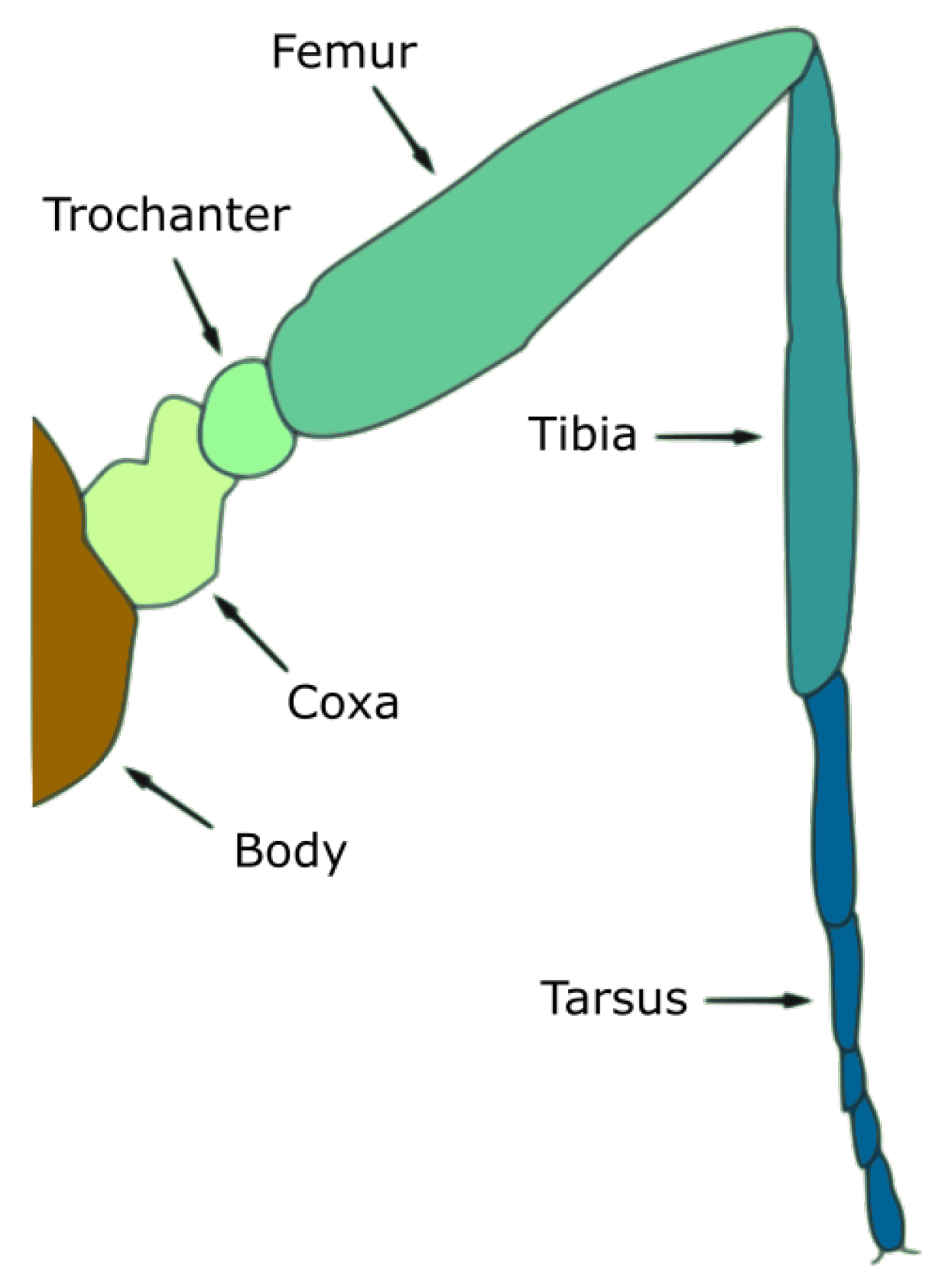
The design of the leg is inspired by insect leg structure so the robot can mimic insect movement patterns. The insect leg consists of five main parts—coxa, trochanter, femur, tibia and tarsus [19]. The insect leg structure is shown in Figure 1. The coxa part is usually less than 10% of the total leg length and is free to rotate with three degrees of freedom within definite limits. The trochanter is even smaller, in the range of 2–8% of the total leg length [20]. Femur and tibia are usually the same size or femur is longer than tibia [21]. Tarsus consists of 3 to 7 segments and its length can vary. The position of each joint depends on the leg position. Front legs have typically different joint positions and link sizes compared to middle or hind legs [22].
Movement of insect leg parts is provided by muscles [24]. Muscle contraction causes a change in leg position. However, muscles have much higher power to mass ratios compared to electric motors and servos. Furthermore, joints can typically move in multiple degrees of freedom. Electric motors and servos have typically only one degree of freedom.
All these aspects must be reflected when designing an artificial insect leg. Some characteristics can be replicated, others must be adjusted. We wanted to get as close as possible to the ratio of the parts of the insect leg. However, we were limited by the dimensions of the servomotors.
Another requirement when designing the limb and selecting the proper components was the payload capacity of the robot. The goal was that the robot would be able to carry a load of its own weight.
The resulting dimensions of the robot were adjusted to the size of the designed leg. The dimensions of the robot’s body had to ensure that the individual legs were placed far enough apart and could move freely in the defined areas. The robot is 58 cm long, its height ranges from 15.5 cm to 48.5 cm and its width ranges from 23 cm to 96 cm, depending on the current stance.
Bio-inspired robots have three basic leg placements inspired by mammals, spiders and reptiles [25]. Thanks to the design of the legs, our robot is able to use both spider and reptile placements.
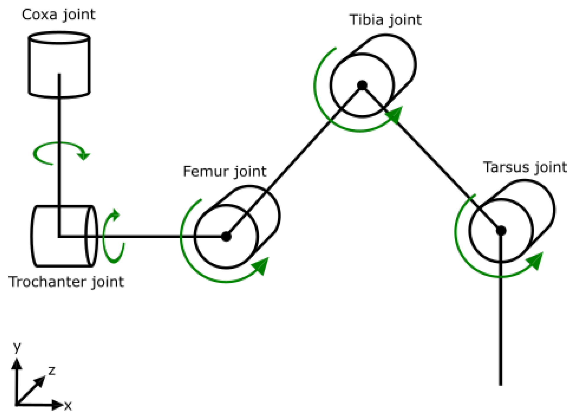
The leg of our robot consists of five main parts. The design is similar to insect leg structure. The dimensions of the leg parts are in Table 2. The total length of the leg is 483 mm. The coxa part is larger than 10% of the leg length, because the leg needs to rotate in a full 180 degrees radius. The trochanter is also beyond the expected size, because the joint requires a stronger servomotor, with large dimensions. Femur and tibia parts are the longest parts of the leg as they should be. Tarsus length can be adjusted as needed. The scheme of the leg is in Figure 2.
Each joint is operated by one Dynamixel servomotor (see Table 2 for details) [26]. Trochanter and femur joints require the most power compared to other joints, so the MX-106 servomotors were used. Coxa, tibia and tarsus joints do not require as much power as trochanter and femur joints, so the MX-64 servomotors were used. Both servomotor types have the same nominal voltage of 12 V and can be powered by a power supply or a battery.
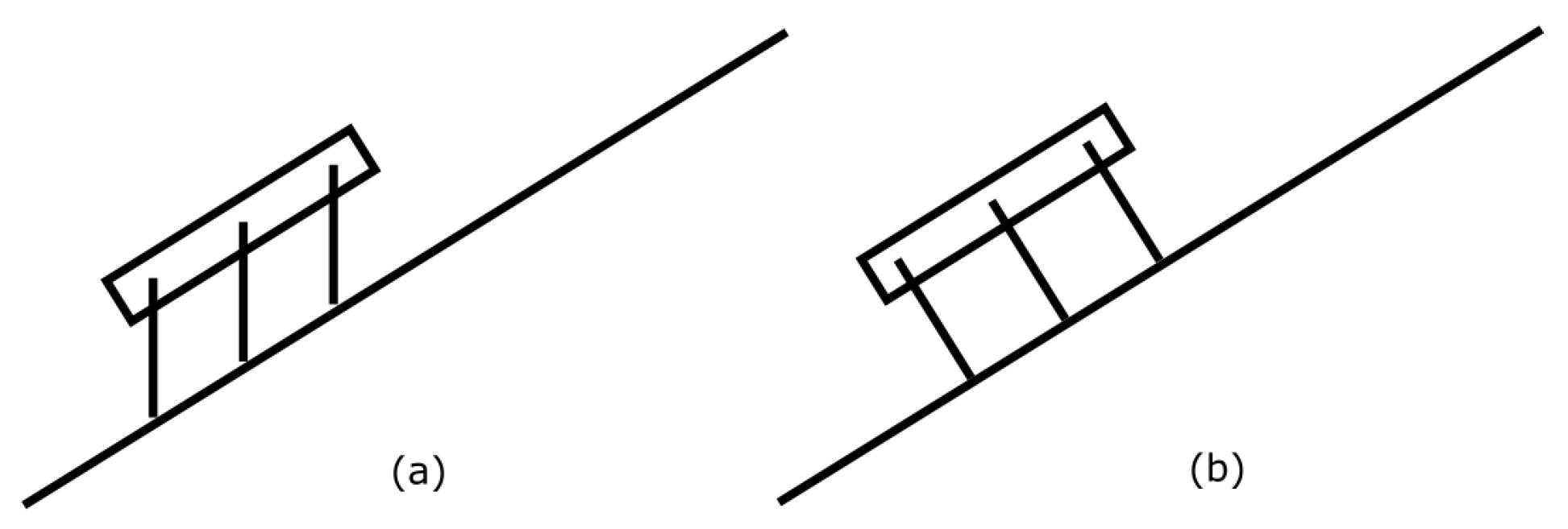
Most hexapod robots have only three leg parts and, thus, only three degrees of freedom—coxa, femur and tibia. Although, three joints are enough for fluent walk, the additional joints can be used for various tasks, such as object manipulation. A robot with more degrees of freedom can also move in more stances than a hexapod with three degrees of freedom, which increases the ability of the robot to avoid obstacles or traverse rough terrain. The trochanter joint is the most uncommon joint for hexapod robots, even though it can be used for better stabilization on inclined terrains. The leg can be rotated and positioned parallel to the gravitational force which takes load from the coxa joint and reduces its energy consumption. This situation is shown in Figure 3.
2.1. Forward Kinematics
The forward kinematics of the leg is based on the Denavit–Hartenberg (DH) convention (the Denavit–Hartenberg leg parameters are shown in Table 3). The transformation matrix DH between the coordinate systems of adjacent legs is given by Equation (1):
where denotes , denotes and the DH parameters , , and are the rotation around z, translation along z, translation along x and rotation around x, respectively. The mapping between the global coordinate system and the foot tip coordinate system is given by Equation (2):
where f is the foot tip frame.
2.2. Inverse Kinematics
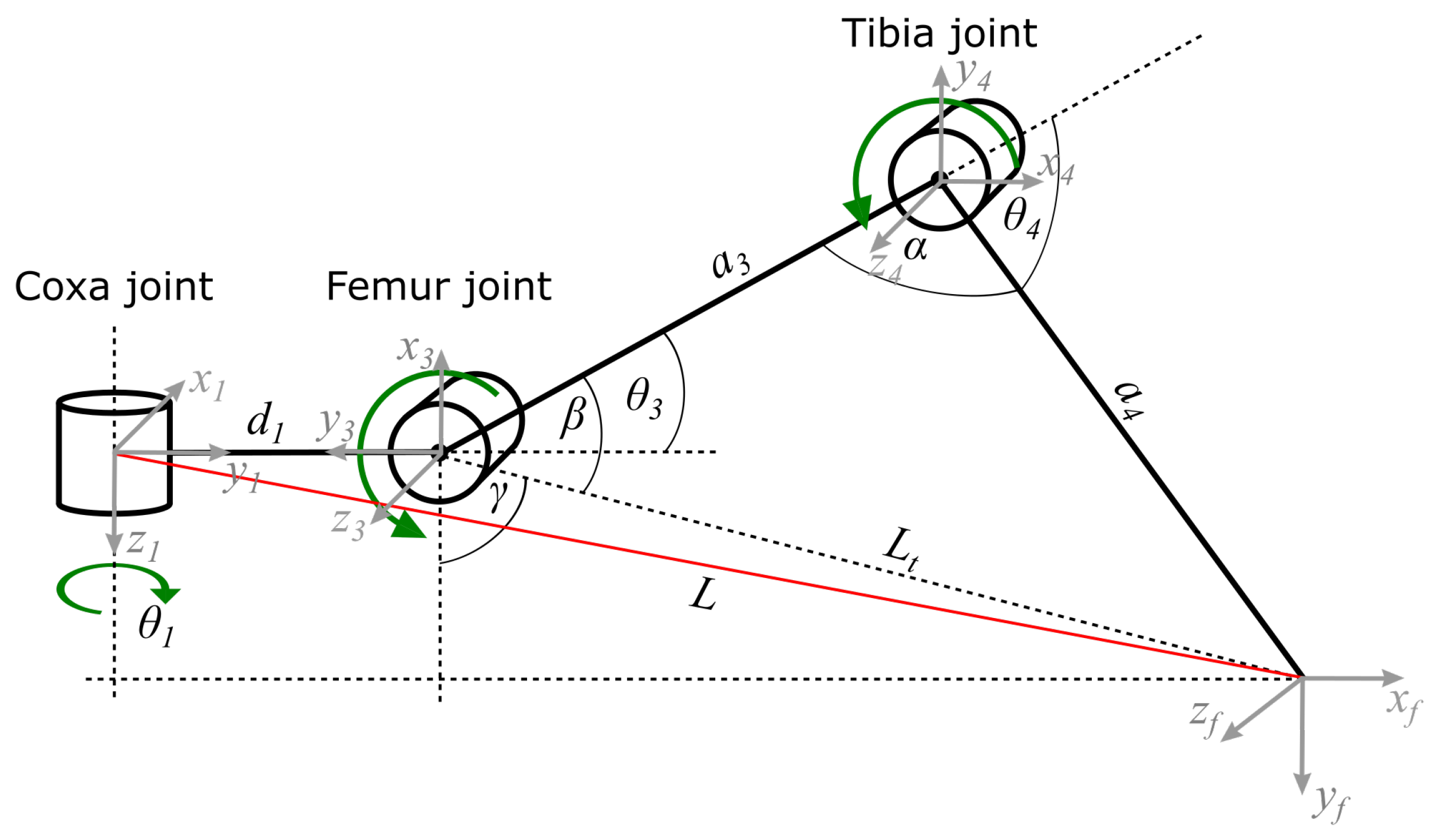
The inverse kinematics task is to find joint angles based on the position of the foot tip for all legs l. Due to the five degrees of freedom the solution is under-determined. One solution is to add a constraint as in [9]. However, we preferred the reduction of controlled degrees of freedom of the leg. The control of the trochanter joint is based on data from the inertial measurement unit, which senses the tilt of the robot’s body, and the tarsus joint is controlled by the reflexive layer that keeps the joint parallel to the gravitational force. The resulting system has only three degrees of freedom. The inverse kinematics can then be solved using the following Equations (3)–(10). The established coordinate system is shown in Figure 4.
where , and are the foot tip coordinates, is coxa length, is femur length, is tibia length, L is the distance between coxa joint and the foot tip, is the distance between femur joint and the foot tip and , and are the angles for coxa, femur and tibia joints.
3. Robot Locomotion
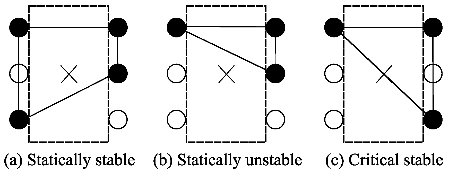
When planning the robot’s movement, an important aspect is its stability. A legged robot can be in two different states of stability—dynamic or static. A statically-stable robot is in a stable position at every moment of its motion, which means that its center of gravity must be located in the polygon formed by the legs that are currently providing support. A statically-unstable robot is not in a stable position at every moment of its motion. This can be expressed as the center of gravity being outside the polygon of the supporting legs, which means the robot is basically falling. Between these two stability states, there is a critically stable position where the robot balances between the previous two states (see Figure 5). However, a statically-unstable robot can become dynamically stable if additional force is supplied, e.g., by moving a leg [28,29].
The selection of the appropriate gait depends on the desired performance characteristics, such as speed, stability or power consumption, but also on the size and shape of the robot or the complexity of the terrain [17].
There are several indices for comparing walking robots of different sizes, shapes and masses. One of them is the duty factor [30], which is defined by Equation (11). Duty factor can also be used to distinguish between running and walking, where is for running and is for walking [25].
where is time when the leg provides support and is duration of one step.
The most commonly used gaits can be seen in insects, such as tripod, wave or ripple [31]. The tripod gait is one of the fastest gaits. It is a regular, periodic gait, where , which is on the border of running [25]. The tripod is the most suitable gait for use on flat terrain because it is fast but has relatively low stability. In contrast, the wave is the most stable gait because only one leg is moving at any given time (). It is also the slowest gait. The ripple gait allows movement at medium speed while maintaining relatively high stability. A maximum of two legs are moving at the same time.
Figure 5.
Robot stability during movement. The supporting leg is shown in black, X represents the robot’s center of gravity. (a) The statically-stable robot has a centre of gravity inside a polygon formed by the supporting legs. (b) A statically-unstable robot does not have a center of gravity inside the polygon formed by the supporting legs and, thus, the robot is in danger of falling. (c) The robot balances at the edge of stability, which is expressed by the centre of gravity at the edge of the polygon formed by the supporting legs. The figure is inspired by [32].

Movement Controller
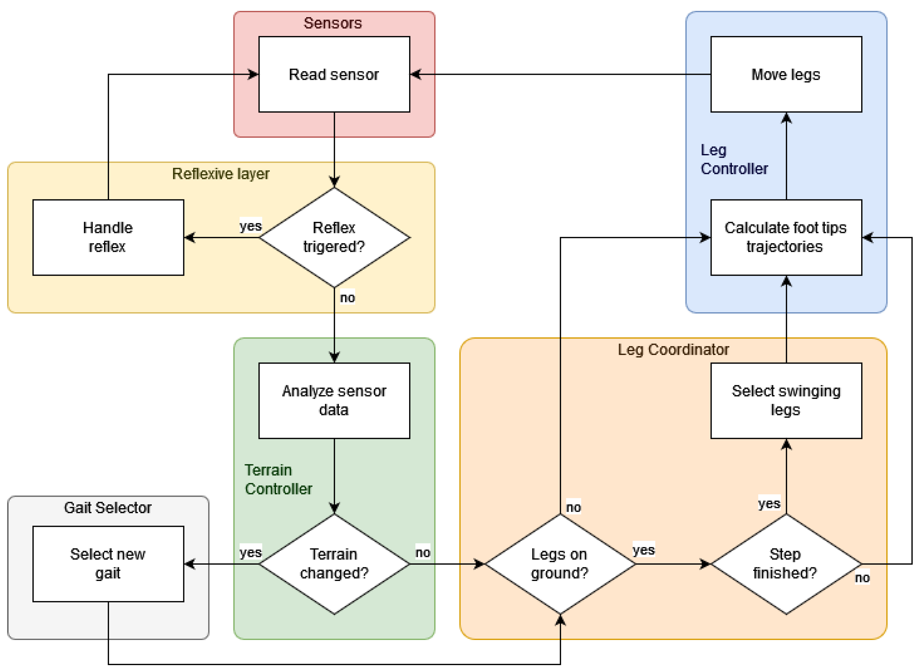
The movement controller adapts the used gait to the current terrain conditions. It consists of five main blocks—reflexive layer, terrain controller, gait selector, leg coordinator and leg controllers (see Figure 6). The controller was described in detail in previous work [18].
Sensor data are processed by the reflexive layer, which, eventually, triggers the reflexive behavior of the robot by sending direct commands to the leg controller. Unless one of the reflexes is activated, data from the sensors is sent to the terrain controller, which analyzes the roughness of the terrain. The most suitable gait is then selected by the gait selector based on the terrain analysis. The resulting gait is obtained by the leg coordinator and executed by the leg controllers.
The reflexive layer triggers three reflexes [13]. The stepping reflex moves the leg closer to the body, reducing energy consumption and increasing the stability of the robot. The elevator reflex is triggered when the leg encounters an obstacle during its movements, whereby it tries to repeat the movement with an increased step height. The search reflex is activated if the leg does not find the support at the expected location. It searches for another support in the surrounding area.
4. Materials and Methods
To verify the proposed robot and controller design, a series of experiments were performed. The movement speed and energy consumption were tested using tripod gait and all six wheels, on both flat and sloping terrain.
The inclined terrain was simulated by a wooden board with an adjustable slope. The robot was powered by a 12 V power supply. The servomotors were controlled by an U2D2 controller [33]. The load on the individual servomotors was measured as the current flowing through the servomotor. The actual current of each servomotor was read from the servomotor registers. Another way to measure the load on the servomotors would be the usage of an external current sensor. However, one sensor would need to be attached to each servomotor, which would be very complicated. In addition, the servomotors themselves measure their current with a resolution of 3.36 mA, which was sufficient accuracy for the experiment. The total current of the robot was measured at 50 Hz using a hall effect-based linear current sensor, ACS712, which was connected to the Arduino Mega board.
4.1. Reading Data from Servomotors
The servomotors used for the individual robot joints are controlled by TTL half duplex asynchronous serial communication, which is implemented over a single wire [34]. Its baud rate can be set from 8000 bps to 4.5 Mbps. The 1 Mbps speed was eventually chosen, because higher speeds caused a high number of communication errors. Protocol version 2.0 was used for communication. Unlike the protocol version 1.0, it has the possibility to read or write to multiple servomotors simultaneously using the sync read and sync write methods [35]. Sync methods allow the reading of data from several servomotors by sending one instruction packet. Each servomotor responds with a status packet. The use of the sync read method reduces the traffic on the communication link. Values can, thus, be read more frequently than with sequential reading.
When using a higher baud rate, it is also necessary to reduce the latency of the USB port. We set the USB port latency to 1 ms. The bus speed is also affected by the response time of the individual servomotors [36]. The response time can be set in the Return Delay Time register. The default value was 250 μs. This value was reduced up to 20 μs. Furthermore, the Profile Acceleration register value was set to 20, the Profile Velocity register value was set to 5000 and the Position P Gain register value was set to 850. These modifications increased the smoothness of movement of the individual servomotors and, thus, the movement smoothness and stability of the whole robot.
4.2. Speed and Power Consumption on Sloping Terrain
The goal in this experiment was to analyze the power consumption of the servomotors in different stances and movements and to verify that the trochanter joint reduces the load on the other joints when the robot is standing, walking and riding on inclined terrain.
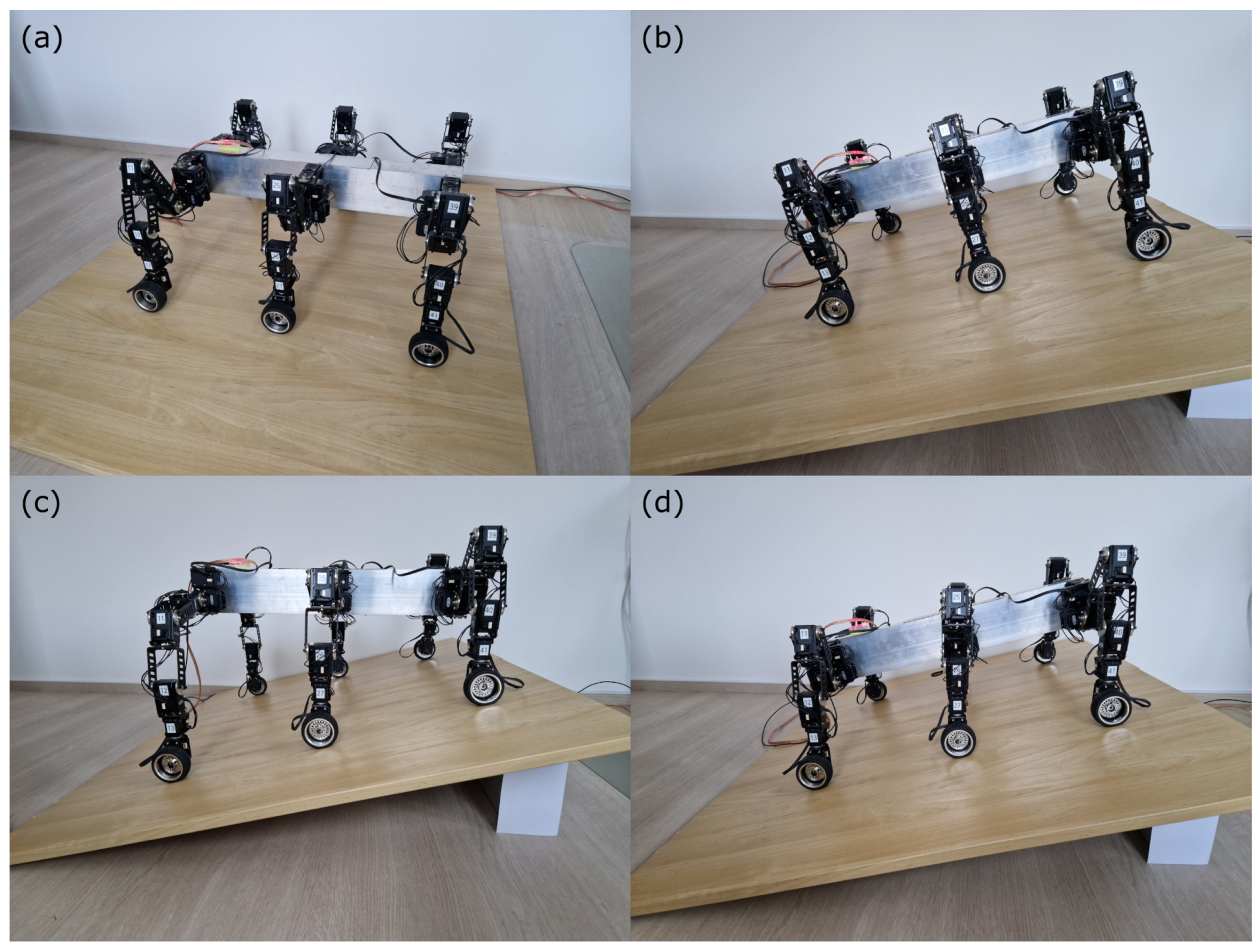
Three different static stances and two movements (tripod gait with a maximum speed of 0.12 m/s and a period of 1.6 s and ride using six wheels with a maximum speed of 0.2 m/s) were tested at six different inclinations (see Table 4). All tested stances were based on the robot’s default stance (Figure 7a). The first derived stance (No. 1) did not use the trochanter joint and all limbs were at the same height (Figure 7b). The second derived stance (No. 2) also did not use the trochanter joint, but the individual limbs were at different heights that corresponded to the slope of the tested terrain (Figure 7c). Finally, the third derived stance (No. 3) used the trochanter joint and all limbs were at the same height. The angle of rotation of the trochanter joint was identical to the slope of the tested terrain (Figure 7d).
Each stance was measured three times. Measurements of static stance contained 40 values, which were then averaged. Measurements of the moving robot were collected at a frequency of 50 Hz. In some cases, the servomotor did not respond within the specified limit or the response was corrupted. These occurrences were removed from each measurement. The resulting value of the servomotor current was determined according to Equation (12).
where is the current of the servomotor with ID s, is the ith value of the measurement and n is the count of accepted values in the measurement.
The resulting total leg current was given by Equation (13).
where is the total current of the leg with ID l, is the current of the servomotor with ID s and m is count of servomotors in the leg.
The resulting current for the given stance was determined using Equation (14).
where I is the resulting current of the given stance and is the current of the leg with ID l.
The power indicator energetic cost of transport (CoT) was used to compare the energy consumption with other robots. It is defined as the energy required to move a unit mass over a unit distance [37,38]. By substituting energy for power, we can write CoT as Equation (15):
where P is the power consumed by the robot during the motion, m is the mass of the robot and v is the speed of the robot. The power can then be determined by Equation (16):
where U is the supply voltage of the robot and I is the current drawn from the power supply.
5. Results
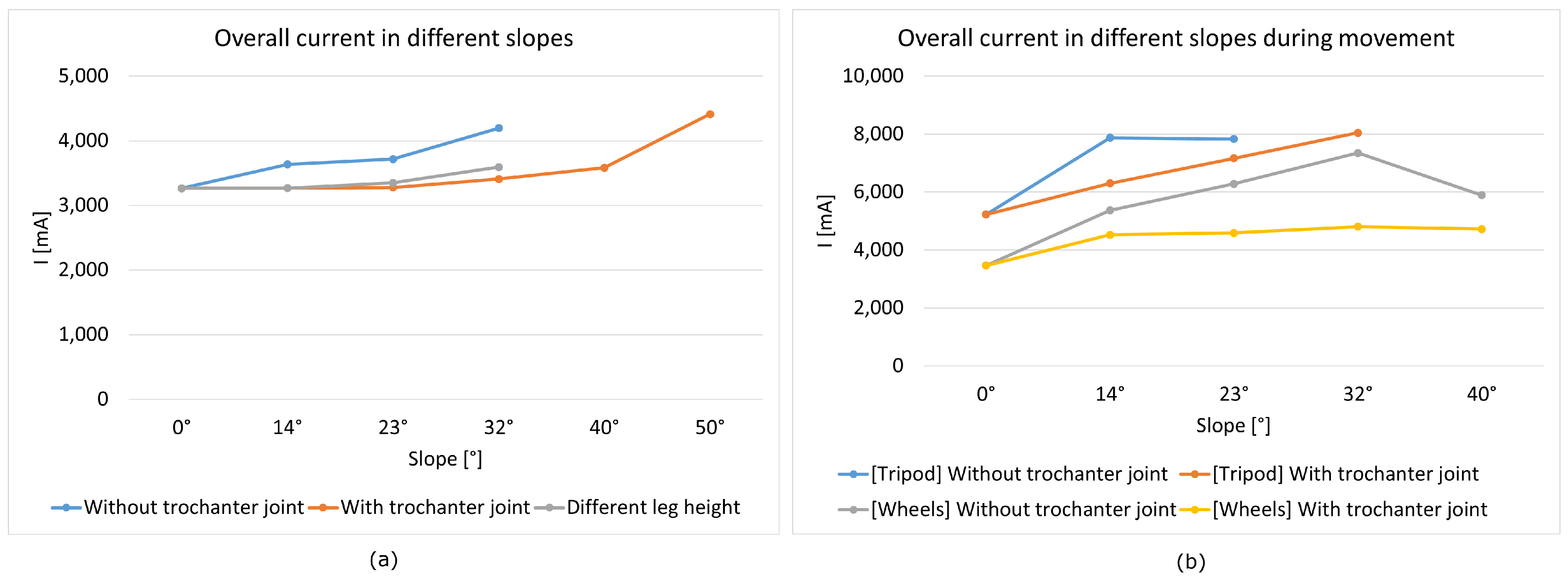
All measurements were calculated according to the methodology presented in Section 4.2. The results for each stance and movement are shown in the following charts. Figure 8a shows a chart of the total current of the robot at three static stances. The stance using the trochanter joint had the lowest current value and, therefore, the lowest power consumption. The stance with different leg heights had low energy requirements compared to the stance that did not use the trochanter joint, which had a significant increase in energy consumption with increasing terrain slope. The stance using the trochanter joint was more than 23% more energy-efficient in the case of a 32° slope.
The chart also shows that the robot was no longer able to stand stably on slopes greater than 32° without the use of a trochanter joint.
Figure 8b shows a chart of the current of the robot during tripod gait and wheeled movement with, and without, the usage of the trochanter joint. Up to 40% energy could be saved when using the wheeled locomotion. When driving on wheels on 40° slopes, there was already considerable slipping. The robot was no longer reliably able to ride on such a slope without using the trochanter joint. This could also be seen in the drop in the current of the robot at an inclination of 40°.
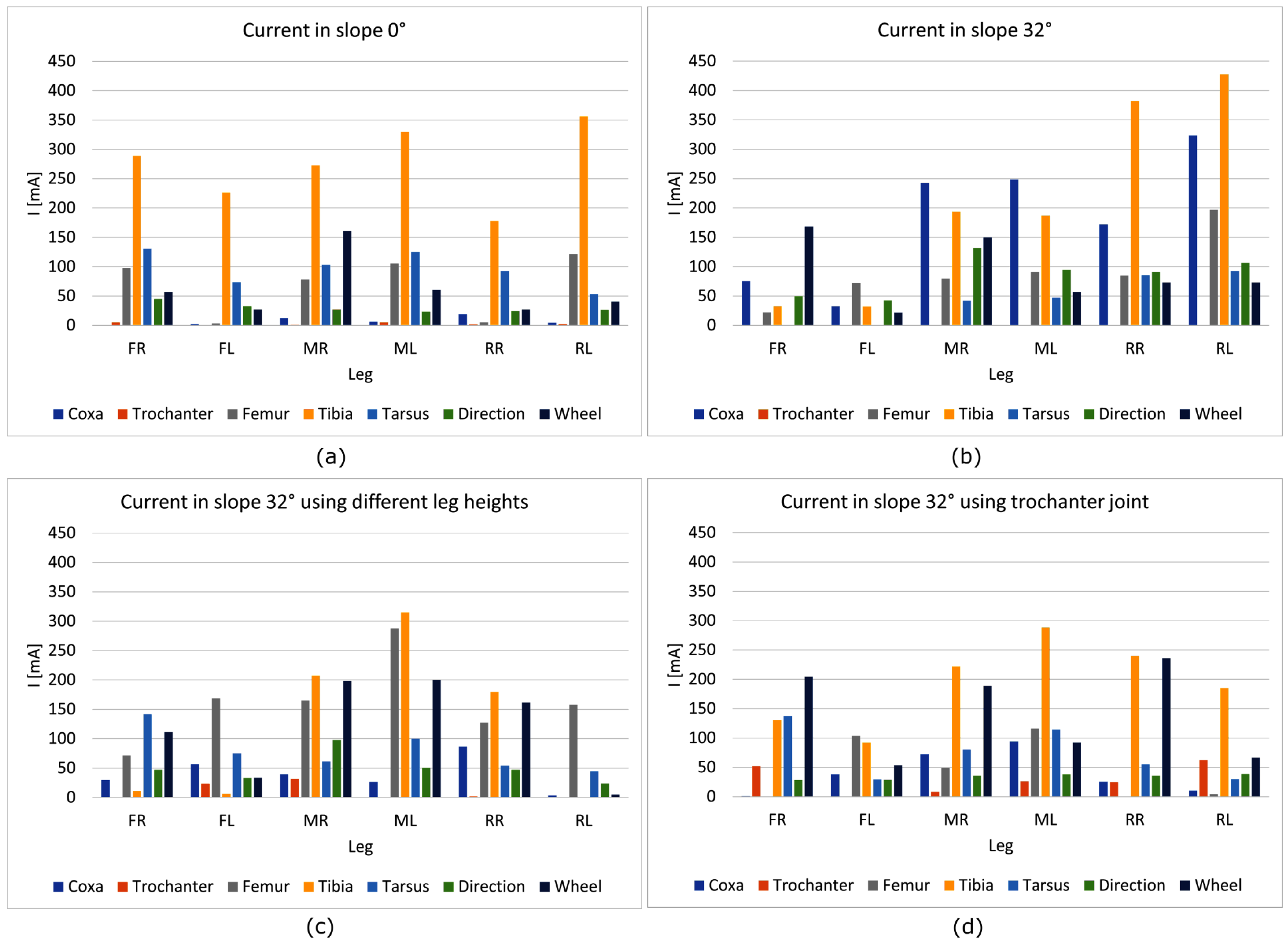
The results are presented in more detail in the graphs, which show the current of individual servomotors of each leg on 0° and 32° terrain slopes for three static stances (see Charts a–d in Figure 9). It can be seen that, as the slope of the terrain increased, the robot’s centre of gravity shifted backwards, increasing the load on the rear limbs. In contrast, the front limbs were loaded significantly less. Furthermore, the coxa servomotors were significantly more loaded when standing without a trochanter joint at a 32° inclination.
The graphs also show uneven loading on the legs. This was mostly due to minor slippage of the limbs on the surface and the tolerance of the controller that controlled the limb loading.
It can also be observed that the difference between the stance using the trochanter joint and the stance with different leg heights was relatively small. It appeared that the use of these stances had similar energy demands. Even so, a robot with a trochanter joint can use more stances and tilting the robot on sloping terrain is easier than using a stance with different leg heights. In the case of our robot, the trochanter joint was also used in case the robot fell on its back. The robot can use the trochanter joint to rotate its limbs by 180 degrees and continue its movement.
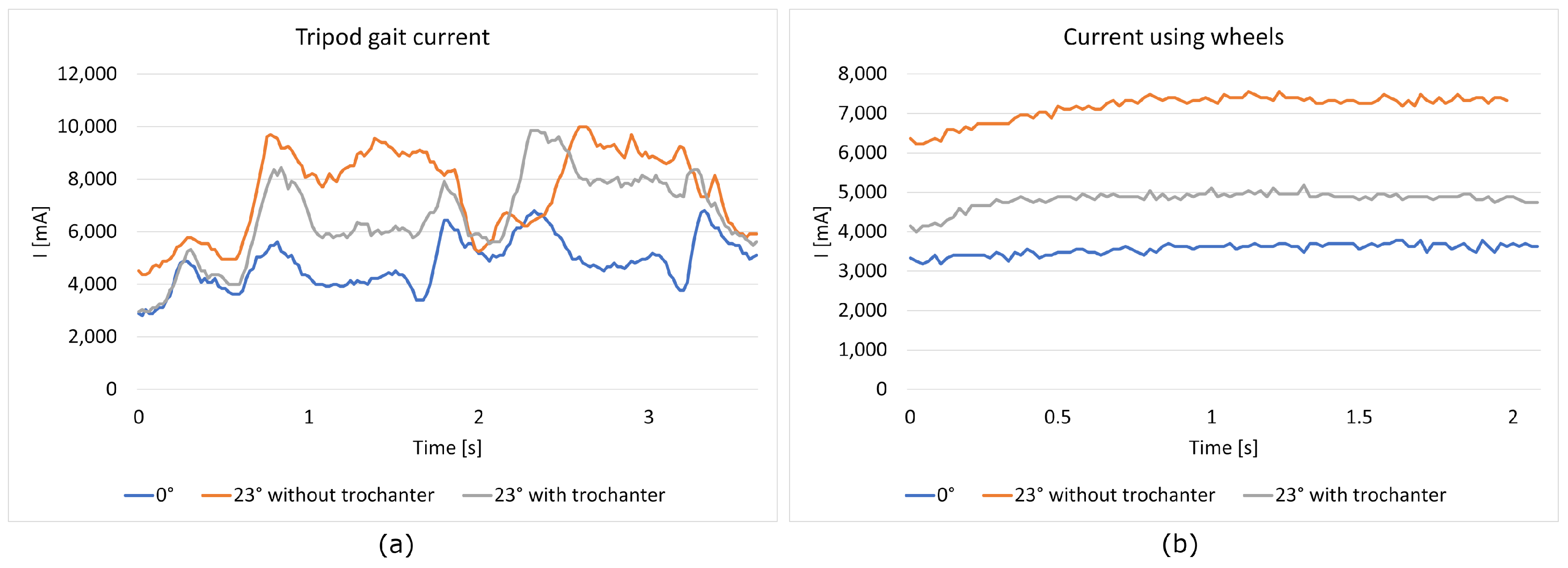
The charts in Figure 10 show the current of the robot when moving using tripod gait and wheeled locomotion with, and without, the use of the trochanter joint on flat terrain and on a 23° slope. The speed of the tripod gait ranged from 0.07 m/s to 0.12 m/s and its period was 1.6 s. The tripod gait on flat terrain had the lowest energy consumption and regular swing phase of the limbs. When walking on sloping terrain, small slips occasionally occurred, especially when using the stance without the trochanter joint.
When using wheels, the energy consumption was constant throughout the movement except for minor fluctuations. At the beginning of the movement, we observed a gradual increase in power consumption caused by the acceleration of the robot. The power consumption when riding on wheels with the trochanter joint was up to 36% lower than when riding without it. The maximum speed of the robot moving by wheeled locomotion was 0.2 m/s.
The power indicator energetic cost of transport (CoT) was used for comparison with other robots. It was calculated with a robot mass of 8.8 kg, power supply voltage of 12 V and a gravitational acceleration of 9.81 m/s2. The CoT for each experiment is given in Table 5. The CoT ranged from 6.05 to 15.97 for the tripod gait and from 2.41 to 5.11 for wheeled locomotion, depending on the slope of the terrain and the usage of the trochanter joint.
6. Discussion
The experiments showed that the proposed limb structure reduces the energy consumption of the robot and allows it to traverse steep slopes that would be impossible for the robot to navigate without the trochanter joint. As can be seen in the charts showing the current of the individual servomotors, using a trochanter joint significantly reduces the load on the coxa joint. There is also better load distribution across all leg servomotors. The energy consumption of the movement is further reduced by the wheeled chassis, which is suitable for movement on flat terrain. In addition, this chassis increases the speed of the robot and can also be used to climb slopes without terrain irregularities. The new limb design also increases the stability of the robot, especially when navigating steep slopes. The experiments showed that, at a certain inclination, the robot is only able to move with the use of a trochanter joint.
The experiments confirmed that the combination of trochanter joint and the terrain controller allows our robot to walk up to an inclination of 32°, to ride inclined terrains up to 40° and remain statically stable on slopes up to 50°. This is an improvement compared to LAURON [39], which is able to walk at an inclination of 25° and stand stably up to 42° and Weaver [9], which is capable of walking up to 30° and remain stable until 50°. Using wheel locomotion, the robot should be able to negotiate steeper slopes. Unfortunately, at higher inclinations of the test bed there was considerable wheel slippage. The same applied for gait movement.
Improvements were also achieved in terms of energy efficiency. The power indicator energetic cost of transport (CoT) on flat terrain was 6.05 when using gait and 2.41 when using wheeled locomotion. In comparison, hexapod Weaver has CoT 15.2 on flat terrain.
7. Conclusions
In this work we presented a bio-inspired hexapod walking robot which has five degrees of freedom per leg. The construction of the leg has a fifth joint that can be used during movement on sloping terrain to increase stability and reduce the energy consumption of the robot. It was experimentally verified with a real robot that the use of a trochanter joint reduces energy consumption during both static stance and movement using gait or wheels. Similar results were achieved in the experiments by adjusting the leg lift to the terrain inclination. However, using a trochanter joint is easier to control and the additional joint can be used for other purposes. Future work will focus on the analysis of individual gaits in relation to their energy requirements and field testing.
Author Contributions
Conceptualization, M.Ž., J.R. and F.V.Z.; methodology, M.Ž. and J.R.; software, M.Ž.; validation, M.Ž., J.R. and F.V.Z.; formal analysis, J.R. and F.V.Z.; investigation, M.Ž.; resources, M.Ž.; data curation, M.Ž.; writing—original draft preparation, M.Ž.; writing—review and editing, M.Ž., J.R. and F.V.Z.; visualization, M.Ž.; supervision, F.V.Z.; project administration, M.Ž. and F.V.Z. All authors have read and agreed to the published version of the manuscript.
Funding
This research was supported by the project IGA FIT-S-23-8151.
Institutional Review Board Statement
Not applicable.
Informed Consent Statement
Not applicable.
Data Availability Statement
No data available.
Conflicts of Interest
The authors declare no conflict of interest. The funders had no role in the design of the study; in the collection, analyses, or interpretation of data; in the writing of the manuscript; or in the decision to publish the results.
References
- Kajita, S.; Espiau, B. Legged robot. In Springer Handbook of Robotics; Springer: Berlin/Heidelberg, Germany, 2008; pp. 361–389. [Google Scholar]
- Elfes, A.; Steindl, R.; Talbot, F.; Kendoul, F.; Sikka, P.; Lowe, T.; Kottege, N.; Bjelonic, M.; Dungavell, R.; Bandyopadhyay, T.; et al. The multilegged autonomous explorer (MAX). In Proceedings of the 2017 IEEE International Conference on Robotics and Automation (ICRA), Singapore, 29 May–3 June 2017; pp. 1050–1057. [Google Scholar]
- Goldschmidt, D.; Hesse, F.; Wörgötter, F.; Manoonpong, P. Biologically Inspired Reactive Climbing Behavior of Hexapod Robots. In Proceedings of the 2012 IEEE/RSJ International Conference on Intelligent Robots and Systems, Vilamoura-Algarve, Portugal, 7–12 October 2012; pp. 4632–4637. [Google Scholar] [CrossRef]
- Belter, D.; Walas, K. A compact walking robot—Flexible research and development platform. In Recent Advances in Automation, Robotics and Measuring Techniques, Proceedings of the International Conference AUTOMATION 2014, Warsaw, Poland, 26–28 March 2014; Springer: Berlin/Heidelberg, Germany, 2014; pp. 343–352. [Google Scholar]
- Gorner, M.; Wimbock, T.; Baumann, A.; Fuchs, M.; Bahls, T.; Grebenstein, M.; Borst, C.; Butterfass, J.; Hirzinger, G. The DLR-Crawler: A testbed for actively compliant hexapod walking based on the fingers of DLR-Hand II. In Proceedings of the 2008 IEEE/RSJ International Conference on Intelligent Robots and Systems, Nice, France, 22–26 September 2008; pp. 1525–1531. [Google Scholar]
- Schneider, A.; Paskarbeit, J.; Schaeffersmann, M.; Schmitz, J. HECTOR, a New Hexapod Robot Platform with Increased Mobility—Control Approach, Design and Communication. In Advances in Autonomous Mini Robots, Proceedings of the 6th International Symposium on Autonomous Minirobots for Research and Edutainment (AMiRE), Bielefeld, Germany, 23–25 May 2011; Rückert, U., Joaquin, S., Felix, W., Eds.; Springer: Berlin/Heidelberg, Germany, 2012; pp. 249–264. [Google Scholar]
- Takubo, T.; Arai, T.; Inoue, K.; Ochi, H.; Konishi, T.; Tsurutani, T.; Hayashibara, Y.; Koyanagi, E. Integrated limb mechanism robot ASTERISK. J. Robot. Mechatron. 2006, 18, 203–214. [Google Scholar] [CrossRef]
- Roennau, A.; Heppner, G.; Nowicki, M.; Dillmann, R. LAURON V: A versatile six-legged walking robot with advanced maneuverability. In Proceedings of the 2014 IEEE/ASME International Conference on Advanced Intelligent Mechatronics, Besacon, France, 8–11 July 2014; pp. 82–87. [Google Scholar]
- Bjelonic, M.; Kottege, N.; Beckerle, P. Proprioceptive control of an over-actuated hexapod robot in unstructured terrain. In Proceedings of the 2016 IEEE/RSJ International Conference on Intelligent Robots and Systems (IROS), Daejeon, Republic of Korea, 9–14 October 2016; pp. 2042–2049. [Google Scholar]
- Henrey, M.; Ahmed, A.; Boscariol, P.; Shannon, L.; Menon, C. Abigaille-III: A versatile, bioinspired hexapod for scaling smooth vertical surfaces. J. Bionic Eng. 2014, 11, 1–17. [Google Scholar] [CrossRef]
- Altendorfer, R.; Moore, N.; Komsuoglu, H.; Buehler, M.; Brown, H.; McMordie, D.; Saranli, U.; Full, R.; Koditschek, D.E. Rhex: A biologically inspired hexapod runner. Auton. Robot. 2001, 11, 207–213. [Google Scholar] [CrossRef] [Green Version]
- Galloway, K.C.; Haynes, G.C.; Ilhan, B.D.; Johnson, A.M.; Knopf, R.; Lynch, G.A.; Plotnick, B.N.; White, M.; Koditschek, D.E. X-RHex: A Highly Mobile Hexapedal Robot for Sensorimotor Tasks; University of Pennsylvania: Philadelphia, PA, USA, 2010. [Google Scholar]
- Espenschied, K.S.; Quinn, R.D.; Beer, R.D.; Chiel, H.J. Biologically based distributed control and local reflexes improve rough terrain locomotion in a hexapod robot. Robot. Auton. Syst. 1996, 18, 59–64. [Google Scholar] [CrossRef]
- Rohmer, E.; Reina, G.; Yoshida, K. Dynamic Simulation-Based Action Planner for a Reconfigurable Hybrid Leg-Wheel Planetary Exploration Rover. Adv. Robot. 2010, 24, 1219–1238. [Google Scholar] [CrossRef]
- Yoshioka, T.; Takubo, T.; Arai, T.; Inoue, K. Hybrid Locomotion of Leg-Wheel ASTERISK H. J. Robot. Mechatron. 2008, 20, 403–412. [Google Scholar] [CrossRef]
- Grand, C.; BenAmar, F.; Plumet, F.; Bidaud, P. Decoupled control of posture and trajectory of the hybrid wheel-legged robot hylos. In Proceedings of the IEEE International Conference on Robotics and Automation, ICRA ’04, New Orleans, LA, USA, 26 April–1 May 2004; Volume 5, pp. 5111–5116. [Google Scholar] [CrossRef]
- Orozco-Magdaleno, E.C.; Gómez-Bravo, F.; Castillo-Castañeda, E.; Carbone, G. Evaluation of Locomotion Performances for a Mecanum-Wheeled Hybrid Hexapod Robot. IEEE/ASME Trans. Mechatron. 2020, 26, 1657–1667. [Google Scholar] [CrossRef]
- Žák, M.; Rozman, J.; Zbořil, F.V. Design and Control of 7-DOF Omni-directional Hexapod Robot. Open Comput. Sci. 2021, 11, 80–89. [Google Scholar] [CrossRef]
- Kojima, T. Developmental mechanism of the tarsus in insect legs. Curr. Opin. Insect Sci. 2017, 19, 36–42. [Google Scholar] [CrossRef] [PubMed]
- Frantsevich, L.; Wang, W. Gimbals in the insect leg. Arthropod Struct. Dev. 2009, 38, 16–30. [Google Scholar] [CrossRef] [PubMed]
- Cruse, H. The function of the legs in the free walking stick insect, Carausius morosus. J. Comp. Physiol. 1976, 112, 235–262. [Google Scholar] [CrossRef] [Green Version]
- Bender, J.A.; Simpson, E.M.; Ritzmann, R.E. Computer-assisted 3D kinematic analysis of all leg joints in walking insects. PLoS ONE 2010, 5, e13617. [Google Scholar] [CrossRef] [PubMed]
- Beeson, N.W. File:InsectLeg.png. 2010. Available online: https://commons.wikimedia.org/wiki/File:InsectLeg.png (accessed on 29 January 2023).
- Smith, D.S. The Structure of Insect Muscles. Insect Ultrastruct. 2012, 2, 111. [Google Scholar]
- Tedeschi, F.; Carbone, G. Design issues for hexapod walking robots. Robotics 2014, 3, 181–206. [Google Scholar] [CrossRef] [Green Version]
- ROBOTIS. Dynamixel MX Series. 2021. Available online: https://emanual.robotis.com/docs/en/dxl/mx/ (accessed on 29 January 2023).
- Duan, X.; Chen, W.; Yu, S.; Liu, J. Tripod gaits planning and kinematics analysis of a hexapod robot. In Proceedings of the 2009 IEEE International Conference on Control and Automation, Christchurch, New Zealand, 9–11 December 2009; pp. 1850–1855. [Google Scholar]
- Belter, D.; Skrzypczyński, P. Integrated Motion Planning for a Hexapod Robot Walking on Rough Terrain. IFAC Proc. Vol. 2011, 44, 6918–6923. [Google Scholar] [CrossRef] [Green Version]
- Zhang, C.D.; Song, S.M. A study of the stability of generalized wave gaits. Math. Biosci. 1993, 115, 1–32. [Google Scholar] [CrossRef] [PubMed]
- Song, S.M.; Choi, B. The optimally stable ranges of 2n-legged wave gaits. IEEE Trans. Syst. Man Cybern. 1990, 20, 888–902. [Google Scholar] [CrossRef]
- Zheng, Y.F. Recent Trends in Mobile Robots; World Scientific: Singapore, 1993; Volume 11. [Google Scholar]
- Mănoiu-Olaru, S.; Nitulescu, M.; Stoian, V. Hexapod robot. Mathematical support for modeling and control. In Proceedings of the 15th International Conference on System Theory, Control and Computing, Sinaia, Romania, 14–16 October 2011; pp. 1–6. [Google Scholar]
- ROBOTIS. U2D2. 2021. Available online: https://emanual.robotis.com/docs/en/parts/interface/u2d2/ (accessed on 29 January 2023).
- ROBOTIS. MX-106T/R(2.0). 2021. Available online: https://emanual.robotis.com/docs/en/dxl/mx/mx-106-2/ (accessed on 29 January 2023).
- ROBOTIS. DYNAMIXEL Protocol 2.0. 2022. Available online: https://emanual.robotis.com/docs/en/dxl/protocol2/ (accessed on 29 January 2023).
- Bestmann, M.; Güldenstein, J.; Zhang, J. High-Frequency Multi Bus Servo and Sensor Communication Using the Dynamixel Protocol. In Proceedings of the RoboCup 2019: Robot World Cup XXIII, Sydney, NSW, Australia, 2–8 July 2019; pp. 16–29. [Google Scholar] [CrossRef]
- Nishii, J. An analytical estimation of the energy cost for legged locomotion. J. Theor. Biol. 2006, 238, 636–645. [Google Scholar] [CrossRef] [Green Version]
- Kottege, N.; Parkinson, C.; Moghadam, P.; Elfes, A.; Singh, S.P. Energetics-informed hexapod gait transitions across terrains. In Proceedings of the 2015 IEEE International Conference on Robotics and Automation (ICRA), Seattle, WA, USA, 26–30 May 2015; pp. 5140–5147. [Google Scholar]
- Roennau, A.; Heppner, G.; Nowicki, M.; Zöllner, J.M.; Dillmann, R. Reactive posture behaviors for stable legged locomotion over steep inclines and large obstacles. In Proceedings of the 2014 IEEE/RSJ International Conference on Intelligent Robots and Systems, Chicago, IL, USA, 14–18 September 2014; pp. 4888–4894. [Google Scholar]
Figure 1.
Insect leg structure. The limb of an insect consists of five parts—coxa, trochanter, femur, tibia and tarsus. Inspired by [23].
Figure 1.
Insect leg structure. The limb of an insect consists of five parts—coxa, trochanter, femur, tibia and tarsus. Inspired by [23].

Figure 2.
Robot leg structure. The leg has five Dynamixel servomotors. Each servomotor operates one joint. The servomotors are powered and controlled using a combined bus that chains the servomotors together and provides both power and serial line interconnection.
Figure 2.
Robot leg structure. The leg has five Dynamixel servomotors. Each servomotor operates one joint. The servomotors are powered and controlled using a combined bus that chains the servomotors together and provides both power and serial line interconnection.

Figure 3.
Usage of trochanter joint on inclined terrain. (a) Our hexapod robot uses trochanter joints on sloping terrain. The leg is set in parallel to the gravitational force. (b) Common hexapod without trochanter joint. The gravitational force adds load to the coxa joint.
Figure 3.
Usage of trochanter joint on inclined terrain. (a) Our hexapod robot uses trochanter joints on sloping terrain. The leg is set in parallel to the gravitational force. (b) Common hexapod without trochanter joint. The gravitational force adds load to the coxa joint.

Figure 4.
The leg coordinate system established for the purposes of inverse kinematic calculations. is coxa length, is femur length, is tibia length, L is the distance between coxa joint and the foot tip, is the distance between femur joint and the foot tip, , and are the angles for coxa, femur and tibia joints, , and are angles used during inverse kinematic calculations and , and are the foot tip coordinates. Both trochanter and tarsus joints are controlled by a reflexive layer and are, thus, not included in the inverse kinematic calculations. Inspired by [27].

Figure 6.
Control flow chart of the robot controller. Sensors provide data to the reflexive layer, that can control leg movement directly in case of reflex activation. Sensor data is also sent to the terrain controller, where the data are transformed and used by the gait selector to determine the most appropriate gait for the current terrain. The chosen gait is executed by the leg coordinator, which controls the leg controllers.

Figure 7.
Robot stances. (a) The default stance. (b) The trochanter joint is not used and the legs have the same height. (c) The trochanter joint is not used, but the leg height is adjusted according to the slope. (d) The angle of rotation of the trochanter joint is adjusted to the slope of the tested terrain.

Figure 8.
Overall current on different slopes for static stances and movements. (a) Static stances: The graph shows that the stance using the trochanter joint and the stance with different leg heights had almost the same energy requirements. In contrast, the basic stance required more and more energy as the terrain slope increased. (b) Tripod and wheel mode: The movement with the usage of the trochanter joint had a lower power consumption in all measured inclinations. The use of a trochanter joint also reduced the power consumption when using wheels.

Figure 9.
Charts of all legs and servomotors for 0° and 32° slopes in different static stances. The graphs show the load on each servomotor of each leg in different terrain slopes using basic stance, stance with different leg heights and stance using the trochanter joint. The abbreviations used for the leg names are as follows: FR—front right, FL—front left, MR—middle right, ML—middle left, RR—rear right, RL—rear left.

Figure 10.
Current during movement in different slopes. (a) Current of the robot when moving using tripod gait with, and without, trochanter joint on 0° and 23° slopes. The chart shows two periods of tripod gait (one period was 1.6 s). Between 0.4 and 2 s, respectively, 2 and 3.6 s, the stance phase was followed by the swing phase of one group of legs and, at the same time, the swing phase was followed by the stance phase of the other group of legs. The maximum speed of the robot using the tripod gait was 0.12 m/s. (b) Current of the robot when moving using wheeled locomotion with, and without, trochanter joint on 0° and 23° slopes. The chart shows the first two seconds of the movement. In the first part, the robot accelerated to its maximum speed and the current gradually increased. In the second part, the speed of the robot no longer changed and the current oscillated around a constant value. The maximum speed of the robot using the wheeled locomotion was 0.2 m/s.


Table 1.
Comparison of legged robots.
| Robot | Leg DOF | Dimensions | Mass | Speed | Coxa | Trochanter | Femur | Tibia | Tarsus |
|---|---|---|---|---|---|---|---|---|---|
| L × W × H | [kg] | [m/s] | [m] | [m] | [m] | [m] | [m] | ||
| MAX | 3 | 2.4 × 2.1 × 2.3 | 60.0 | 0.08 | 0.8 | 1.5 | |||
| AMOS II | 3 | 0.5 × 0.4 × 0.1 | 4.2 | 0.035 | 0.06 | 0.115 | |||
| Messor II | 3 | 0.5 × 0.5 × 0.2 | 2.6 | ||||||
| DLR-Crawler | 4 | 0.5 × 0.5 × 0.2 | 3.5 | 0.20 | 0 | 0.075 | 0.04 | 0.04 | |
| Hector | 3 | 13.0 | 0.032 | 0.26 | 0.28 | ||||
| ASTERISK | 4 | 4.0 | 0.07 | 0.05 | 0.105 | 0.105 | |||
| Lauron V | 4 | 0.9 × 0.8 × 0.7 | 43.5 | 0.14 | |||||
| Weaver | 5 | 0.6 × 0.6 × 0.3 | 7.0 | 0.12 | 0.067 | 0.062 | 0.107 | 0.088 | 0.135 |
| Our hexapod | 5 | 0.6 × 0.6 × 0.4 | 8.8 | 0.12 / 0.2 | 0.073 | 0.064 | 0.127 | 0.124 | 0.095 |
| Abigaille-III | 3 | 0.2 × 0.2 × 0.1 | 0.6 | 0.001 | 0 | 0.03 | 0.03 | ||
| R-Hex | 1 | 0.5 × 0.4 × 0.1 | 7.0 | 0.55 | 0.175 | ||||
| X-RHex | 1 | 0.6 × 0.4 × 0.1 | 9.5 | 1.54 | 0.175 | ||||
| ASTERISK-H | 3 | 3.4 | ? / 0.30 | ||||||
| Cassino III | 2 | 0.4 × 0.2 × 0.2 | 0.02 / 0.15 |
† The second number indicates the speed when using the wheels. ‡ Coxa and femur joints are united.
Table 2.
Dimensions of the robot leg. The table shows the dimensions of each part of the robot leg and the models of motors used for each joint. The whole limb measures 483 mm.
Table 2.
Dimensions of the robot leg. The table shows the dimensions of each part of the robot leg and the models of motors used for each joint. The whole limb measures 483 mm.
| Part | Length [mm] | % of the Total Leg Length | Dynamixel Servomotor |
|---|---|---|---|
| coxa | 73 | 15.11 | MX-64 |
| trochanter | 64 | 13.25 | MX-106 |
| femur | 127 | 26.29 | MX-106 |
| tibia | 124 | 25.67 | MX-64 |
| tarsus | 95 | 19.67 | MX-64 |
Table 3.
Values of the Denavit–Hartenberg parameters of the leg.
| Link | i | ||||
|---|---|---|---|---|---|
| [mm] | [mm] | [rad] | [rad] | ||
| coxa | 1 | 65 | 0 | ||
| trochanter | 2 | 22 | 0 | ||
| femur | 3 | 0 | 127 | 0 | |
| tibia | 4 | 0 | 124 | 0 | |
| tarsus | 5 | 0 | 95 | 0 |
Table 4.
The parameters of the proposed experiments. This table describes the parameters of each experiment, specifically the slope of the terrain, the stance used and its characteristics. Each experiment was performed for static stance, walking using tripod gait and driving all six wheels.
Table 4.
The parameters of the proposed experiments. This table describes the parameters of each experiment, specifically the slope of the terrain, the stance used and its characteristics. Each experiment was performed for static stance, walking using tripod gait and driving all six wheels.
| Terrain Slope [°] | Stance Number | Trochanter Joint Angle [°] | Limbs Posture |
|---|---|---|---|
| 0 | 1 | 0 | same height |
| 14 | 1 | 0 | same height |
| 14 | 2 | 0 | different height |
| 14 | 3 | 14 | same height |
| 23 | 1 | 0 | same height |
| 23 | 2 | 0 | different height |
| 23 | 3 | 23 | same height |
| 32 | 1 | 0 | same height |
| 32 | 2 | 0 | different height |
| 32 | 3 | 32 | same height |
| 40 | 1 | 0 | same height |
| 40 | 2 | 0 | different height |
| 40 | 3 | 40 | same height |
| 50 | 1 | 0 | same height |
| 50 | 2 | 0 | different height |
| 50 | 3 | 50 | same height |
† In terrain with zero slope, there was no point in testing the other two stances because they corresponded to stance number 1.
Table 5.
The power indicator energetic cost of transport for both tripod gait and wheeled locomotion on different slopes.
Table 5.
The power indicator energetic cost of transport for both tripod gait and wheeled locomotion on different slopes.
| Movement | Slope | Speed | Current | Current T | CoT | CoT T |
|---|---|---|---|---|---|---|
| tripod | 0 | 0.12 | 5.22 | - | 6.05 | - |
| tripod | 14 | 0.12 | 7.87 | 6.30 | 9.12 | 7.30 |
| tripod | 23 | 0.10 | 7.83 | 7.16 | 10.88 | 9.95 |
| tripod | 32 | 0.07 | - | 8.04 | - | 15.97 |
| wheels | 0 | 0.20 | 3.47 | - | 2.41 | - |
| wheels | 14 | 0.20 | 5.37 | 4.52 | 3.73 | 3.14 |
| wheels | 23 | 0.20 | 6.29 | 4.59 | 4.37 | 3.19 |
| wheels | 32 | 0.20 | 7.35 | 4.80 | 5.11 | 3.34 |
| wheels | 40 | 0.15 | - | 4.72 | - | 4.37 |
† without using the trochanter joint; ‡ using the trochanter joint.
Disclaimer/Publisher’s Note: The statements, opinions and data contained in all publications are solely those of the individual author(s) and contributor(s) and not of MDPI and/or the editor(s). MDPI and/or the editor(s) disclaim responsibility for any injury to people or property resulting from any ideas, methods, instructions or products referred to in the content. |
© 2023 by the authors. Licensee MDPI, Basel, Switzerland. This article is an open access article distributed under the terms and conditions of the Creative Commons Attribution (CC BY) license (https://creativecommons.org/licenses/by/4.0/).
Share and Cite
MDPI and ACS Style
Žák, M.; Rozman, J.; Zbořil, F.V. Energy Efficiency of a Wheeled Bio-Inspired Hexapod Walking Robot in Sloping Terrain. Robotics 2023, 12, 42. https://doi.org/10.3390/robotics12020042
AMA Style
Žák M, Rozman J, Zbořil FV. Energy Efficiency of a Wheeled Bio-Inspired Hexapod Walking Robot in Sloping Terrain. Robotics. 2023; 12(2):42. https://doi.org/10.3390/robotics12020042
Chicago/Turabian StyleŽák, Marek, Jaroslav Rozman, and František V. Zbořil. 2023. "Energy Efficiency of a Wheeled Bio-Inspired Hexapod Walking Robot in Sloping Terrain" Robotics 12, no. 2: 42. https://doi.org/10.3390/robotics12020042
Note that from the first issue of 2016, this journal uses article numbers instead of page numbers. See further details here.