

Global Path Planning Method Based on a Modification of the Wavefront Algorithm for Ground Mobile Robots
by
 , , , and
Martin Psotka
1,
František Duchoň
1,*,
Mykhailyshyn Roman
2,3 ,
,
Tölgyessy Michal
1 and
Dobiš Michal
1 1
Institute of Robotics and Cybernetics, Faculty of Electrical Engineering and Information Technology, Slovak University of Technology, 811 07 Bratislava, Slovakia
2
Texas Robotics, College of Natural Sciences and the Cockrell School of Engineering, The University of Texas at Austin, Austin, TX 78712, USA
3
Department of Automation of Technological Processes and Manufacturing, Ternopil Ivan Puluj National Technical University, 46001 Ternopil, Ukraine
*
Author to whom correspondence should be addressed.
Robotics 2023, 12(1), 25; https://doi.org/10.3390/robotics12010025
Submission received: 20 January 2023
/
Revised: 2 February 2023
/
Accepted: 6 February 2023
/
Published: 8 February 2023
(This article belongs to the Topic Advances in Mobile Robotics Navigation)
Abstract
:This article is focused on the problematics of path planning, which means finding the optimal path between two points in a known environment with obstacles. The proposed path-planning method uses the wavefront algorithm, and two modifications are implemented and verified. The first modification is the removal of redundant waypoints. The first modification is applied because the wavefront algorithm generates redundant waypoints. These waypoints cause unnecessary changes in the direction of movement. The second one is smoothing the generated trajectory using B-spline curves. The reason for applying the second modification is that trajectory generated by the wavefront algorithm is in the form of the polyline, which is inadequate in terms of the smoothness of the robot’s motion. The verification of the proposed method is performed in environments with different densities of obstacles compared with standard Dijkstra’s and A* algorithms.
1. Introduction
For the safe movement of a mobile robot in the environment, it is necessary to perform two basic activities—localization and navigation. Localization is performed using an environment map and suitable sensors, and SLAM [1,2] is primarily concerned with this issue. The localization, therefore, determines the robot’s position in the environment.
For the collision-free movement of the robot, the so-called reactive navigation is used. This navigation must react fast enough concerning objects in the environment and the robot’s activity. Reactive navigation usually uses only current measurements from sensors and is also called local navigation [3]. The robot’s path planning (i.e., global navigation) is implemented in a known or partially known environment with a predetermined goal. This article focuses on the issue of path planning.
The optimality of the planned path cannot be determined in general [4]. The type of robot chassis used, dimensions, dynamic limitations, etc., are essential. It is also because mobile robots occur in various applications and environments. It depends on these facts and application requirements which path characteristics are crucial and to what extent. The following features are often considered essential in path-planning algorithms:
- The computational complexity also depends on the computational power available to the robot. Currently, some mobile devices are already performing such computing power that in smaller environments and with slower motion, the need for both levels of navigation (global and local) disappear.
- In some cases, the shortest possible path may be preferred, while in other cases, a slightly longer path may be suitable because it has better properties according to another criterion.
- The distance of the path from the obstacles usually expresses the safety of movement. For example, the Voronoi diagram [5] used in path planning ensures the maximum possible distance from all obstacles.
- Physical constraints need to be taken into account. It mainly depends on whether the robot is holonomic. If it is non-holonomic, its radius of rotation must be considered when planning the path.
Moreover, path planning is an optimization problem where different criteria can be applied. According to the [6], four criteria must be considered in a path planning algorithm—optimization (best paths in terms of distance, terrain traversability, energy consumption, or other costs), completeness (all possible solutions for the path), accuracy/precision, and execution time.
Model-based path planning for mobile robots may include knowledge of kinematics (or dynamics), the environment, the planning objective, and available resources [7]. A key aspect in every path-planning method is modeling the environment, its representation (map), and the model of the controlled system itself, i.e., the robot. In general, the following three conditions must be met when creating a map [8]:
- The accuracy of the map must be chosen appropriately given the required accuracy when reaching the target.
- The accuracy of the map and the type of recorded environment properties must correspond to the sensors’ accuracy and ability to capture those properties.
- The complexity of the environment representation is directly proportional to the required computing power or the required computing time.
There are several maps [9,10,11], but it is generally impossible to say which one is the most convenient. The choice depends on the environment and the specific application of the mobile robot. It is also possible to use the advantages of several maps and suppress their disadvantages by creating the so-called hybrid map. The output of path planning is the points on the map where the robot’s direction changes. Reaching these points is the task of reactive navigation, which ensures safe movement or modifies the path to make the movement smoother.
In our research, metric maps were used for robot navigation. In our research, we focus on using metric maps for robot navigation. A metric representation of the environment can use two approaches to cell proximity. In 4-neighbors, we consider only cells in the up, down, right, and left directions adjacent to the current cell. In 8-neighbors, we consider four other cells in diagonal directions as adjacent cells.
The basic algorithms for finding a path in a metric map include the wavefront algorithm, Dijkstra, and A*. The wavefront algorithm [12] considers free space a thermally conductive material with obstacles not being thermally conductive. The individual cells in the metric map are evaluated by spreading the heat between the start and the goal. The optimal path is found by proceeding in the direction of the gradient, respectively against the gradient’s direction.
Dijkstra’s algorithm [13] is typically used on graph structures (topological maps) but can also be used on a metric map (the graph’s vertices create map cells). This algorithm counts all the shortest paths from the specified starting vertex. The points in space represent the graph’s vertices, and the distance between the given points evaluates the edges.
A* [13,14] is a heuristic algorithm that calculates the path from a specified starting point to a defined goal with minimum costs. In path planning in mobile robotics, minimal costs are most commonly used as the shortest path. The points in space also represent the graph’s nodes, and the distance between the given points evaluates the edges. Each point is also assigned a value representing the distance to the goal (e.g., Manhattan distance).
D* (Dynamic A*) [15] is a modification of the A* algorithm used in partially known or dynamically changing environments. It provides a much faster path rescheduling process but at the cost of using a large amount of memory.
One of the characteristic algorithms used on the metric map is the brushfire algorithm [16]. This algorithm assigns values to all map cells depending on the distance to obstacles. It evaluates the cells adjacent to the obstacles and proceeds toward the free space. The values of the map cells express the distance to the nearest obstacle. Based on this evaluation, we can create an array of repulsive forces from obstacles. We can then find the path between the two points by combining repulsive forces from obstacles and attractive forces from the target. The brushfire algorithm is similar to a wavefront algorithm, but its disadvantages are evaluating all free space cells and the local minima problem [16]. The advantage of these algorithms is the possibility of considering the terrain. It can be done by modifying the cost function that evaluates the map cells or using the 3D model of the environment. Our research does not deal with terrain analysis, but the purpose is primarily for indoor mobile robots. Therefore, we assume a flat terrain with the same properties throughout the environment and do not model it. If it is necessary to use the terrain model as well, this issue is discussed, for example, in refs. [17,18].
There are also methods for solving path-planning tasks that use random space searches. The first one is probabilistic roadmaps [19], which consists of two steps forming a graph structure. It consists of vertices and edges. The first step is the learning phase. It generates points (vertices) in free space to cover the free area reasonably. Subsequently, the individual vertices join with the vertices located from them at a specified distance. They can only be connected by edges that ensure a collision-free transition. The second step is the demand phase. This step uses classic graph methods to find the shortest path between the start and the goal. There must be a path from the start and goal to other points in the roadmap to find a path.
The second one is rapidly-exploring random trees (RRT) [20]. The trajectory is the rapidly-exploring random tree, which extends from the starting point. The procedure is iterative, while the RRT can be expanded by a fixed distance or a path corresponding to a specified time interval. In each iteration, a vertex in free space is randomly generated. This vertex is then connected to the nearest vertex, providing a collision-free connection. A path (sequence of vertices) connecting the start and goal is selected when one vertex gets close enough to the goal. The advantage of this method is the ability to directly include the kinematic and dynamic constraints of the robot when searching space.
As with probabilistic roadmaps, the genetic algorithm [21] can search the space. Genetic algorithm solutions represent the sequence of visited transition points, starting at the start and ending at the goal. The solution’s success is expressed by the value of the fitness function, which can include the total length of the path, the distance from obstacles, and more. The sequences, commonly named chromosomes, are initialized randomly. They are modified using the so-called genetic operations (crossover, mutation), and better solutions are selected for the next generation. When finished, the solution is the best sequence found.
The advantage of random space searching methods is the ability to achieve good (suboptimal) results with low computational complexity. The main disadvantage is that they usually do not generate an optimal path in terms of path length, and the smoothness of the path is also reduced.
In general, the topic of global path planning is pretty extensive, and it is not possible to provide and analyze all aspects in the introduction of this article. More details can be found in [22].
The article is divided as follows. Section 2 describes the prerequisites we used in our research and development of the path-planning method. It also describes this proposed approach. Section 3 describes different simulation results and presents different comparison criteria of three path-planning methods with three criteria and their multi-criteria combination. At the end of the article, there is a summary and proof that the proposed path-planning method is usable and comparable to state-of-the-art methods.
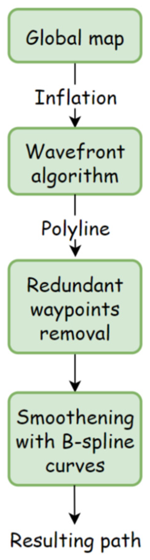
2. Materials and Methods
Global navigation algorithms on a metric map commonly produce trajectories containing breakpoints. The direction of movement changes sharply at this point, which is inadequate in terms of the smoothness of the robot’s movement (e.g., the sum of changes in rotation during the path execution). Therefore, it is appropriate to create a curve based on the breakpoints, which will compromise the exact achievement of the given points and the ideal curve shape from the dynamics point of view of the mobile robot. It can be achieved, for example, by using B-spline curves [23].
B-spline curves are approximation curves that result from polynomial interpolation. Unlike Bézier curves, which are defined as point interpolation, B-spline curves are defined as interpolation of so-called basis functions. The degree of basic functions is predetermined and does not depend on the total number of interpolated points. This degree determines from how many points the curves of the basic functions are constructed. B-spline curves are suitable for creating (adjusting) the path of a mobile robot because they are continuous. The degree of their continuity (differentiability) or shape can be easily modified by changing the degree of basic functions or adding control points. Let U = {u0, …, um} be a non-decreasing sequence of real numbers. The elements ui are called knots, and U is a knot vector. Then the i-th basic function of the B-spline curve of zero degree and degree p is defined as [24]:
The basic functions of the zero degree are thus step functions with a value of 1 on a given interval and a value of 0 outside it. The basic functions of degree p, for p > 0, are a linear combination of two basic functions of degree p − 1. The B-spline curve of degree p can then be expressed as:
where Pi are the control points and Ni,p(u) are the basic functions of degree p defined on the node vector:
It contains the first and last node (p + 1)-times. It is so that the curve starts at the first point and ends at the last point. Otherwise, there would be a gap between the first control point and the beginning of the curve and between the end of the curve and the last control point. The number of nodes in the vector U is m + 1, and the number of control points is n + 1, where m = n + p + 1 [25].
Coordinates of the points on the B-spline curve can then be expressed from (3) as:
Pi,x, and Pi,y are the coordinates of the control point Pi. A number of the computed points on the curve can be affected by vector u. This vector contains values from the interval (0, 1) iterated by the inverse number of desired generated points.
Path planning with A* and Dijkstra algorithms is commonly used in ROS [26]. This research proposes the modification of wavefront path planning to be suitable for robot navigation and, in some aspects, better than these commonly used algorithms. The path found by the wavefront algorithm is as close as possible to the obstacles, which follows from the essence of the algorithm. It is also formed by waypoints, in which the robot’s direction changes significantly, which is not very suitable from the point of view of robot position control. Combined with getting too close to the environmental obstacles, this could lead to collisions. Therefore, this modifies the algorithm by providing a greater distance of the generated path from obstacles and smoothens the found path using B-spline curves.
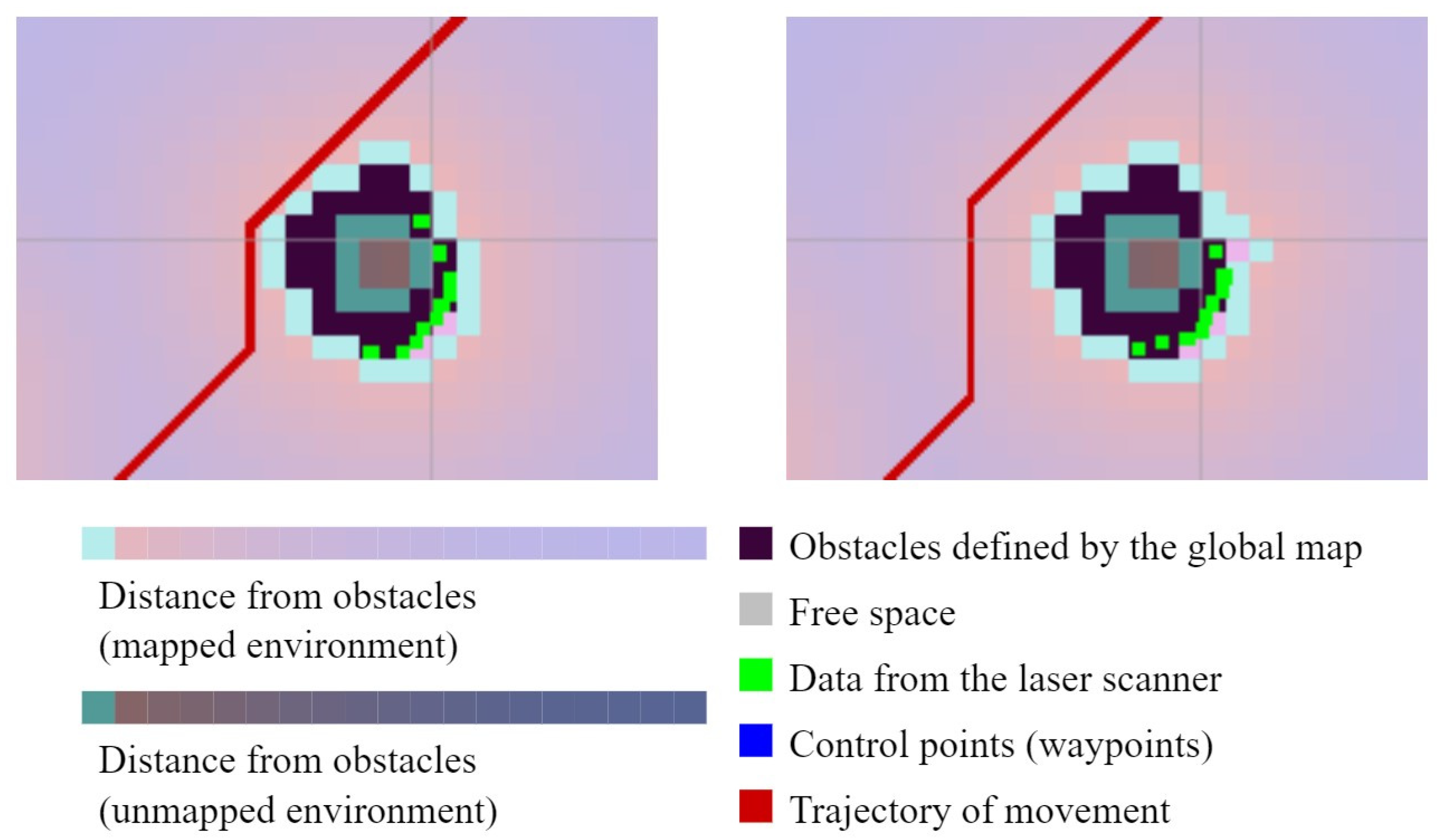
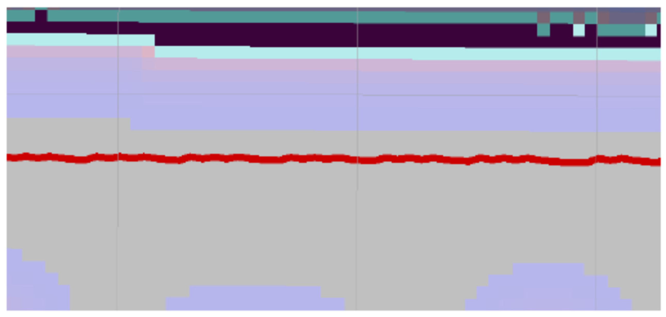
In the first step, obstacles were inflated to ensure sufficient distance to maneuver the robot. This distance can be changed parametrically and set differently for each type of robot. An example of obstacle inflation in the ROS environment can be seen in Figure 1.
The result of the wavefront algorithm is a polyline connecting the start and goal cells on the map, respectively, waypoints on this line, where the robot rotation changes. The centers of the found map cells were determined as waypoints. The path found this way may contain redundant waypoints, which causes more frequent changes of direction. It is due to the wavefront algorithm’s nature and is usually due to the shape or location of the obstacles. Another reason is the searching of neighboring cells, performed in an 8-adjacent, which creates lines at multiples of an angle of 45°. If the robot follows the exact path, then the polyline is unsuitable for robot dynamics. Its direction changes significantly at individual waypoints, which cannot be achieved when moving at a certain speed at a given point. The first step in modifying the original algorithm is to remove redundant waypoints.
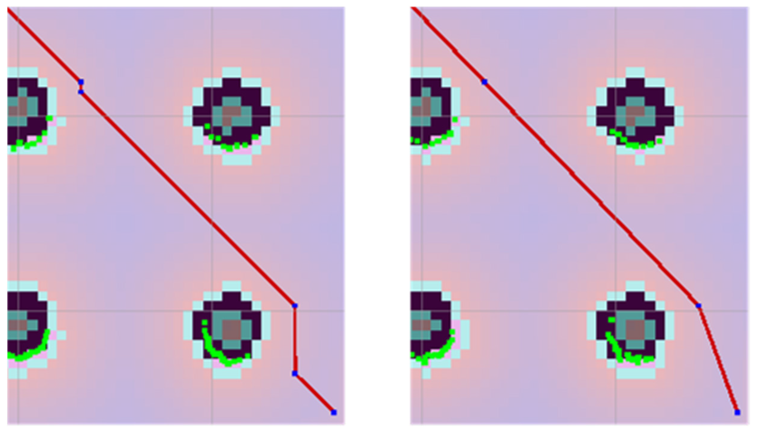
Removing redundant waypoints works on searching all waypoints, and determining the minimum set of these points ensures a collision-free transition through the environment. After removing one of the points, a new line is created on the polyline. The beginning and end of this line are adjacent waypoints to the deleted point. Thus, a given point can only be removed if the adjacent waypoints can be joined by a new line that passes only through the free cells of the map (Figure 2).
An algorithm based on the parametric expression of the line can determine all the map cells through which the generated path passes [27]. Let the two points (beginning and end of the line) be denoted as A = [a1;a2] and B = [b1;b2], the directional vector of the line u = (u1;u2) = B − A and the parametric expression of the line:
Using goniometry, we can calculate the increments for x and y, by which we need to increase the parameter t to move in the given direction by the cell’s dimensions (Δtx, Δty). The variables tx_max and ty_max express the value of the parameter t, in which the line intersects the edge of the cell in the given direction (x, y). These two variables are initialized to the values corresponding to the first intersection of the line with the cell edges in the given direction (x, y), which can be calculated using the parametric equations of the line (6). It is necessary to express the directions in which we move as stepx = sgn(u1) and stepy = sgn (u2). The signs of the components of the direction vector u give these. In this way, it is possible to traverse all the map cells through which the line passes. After each iteration, the current cell is checked, and if we can get to point B, it is clear that all the transition cells are free. In this manner, waypoints and their adjacent waypoints are checked.
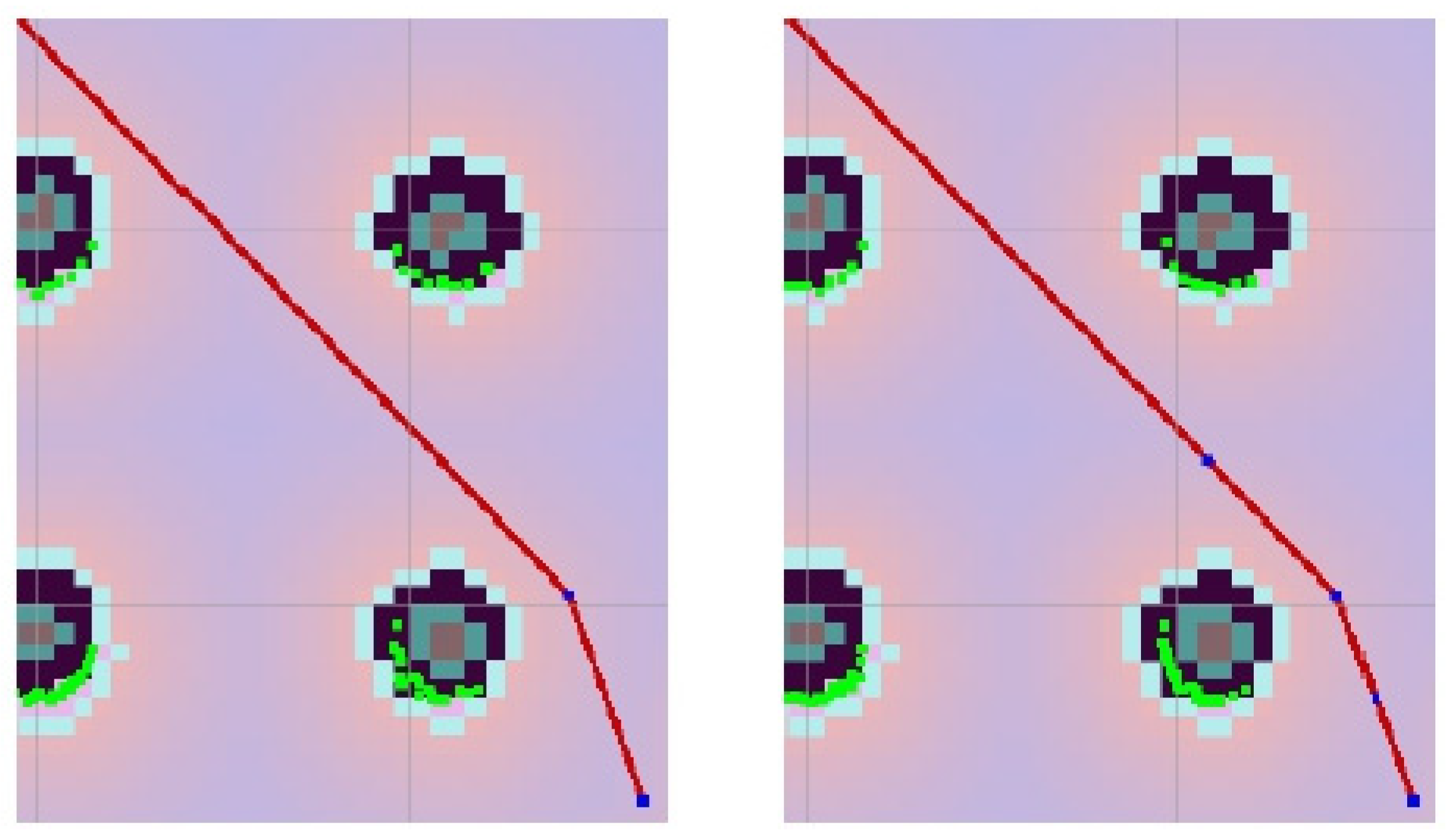
For smoothening, the path B-spline curves were used. The shape of the B-spline curve can be influenced in two ways. The first is the addition of control points, and the second is the use of weights to determine the effect of individual points on the shape of the resulting curve. Control points are considered waypoints, but not all waypoints are control points (Figure 3). For smoothing the path, it is appropriate to use the first option and thus modify the shape of the B-spline curve by adding control points.
In this way, it is possible to limit the maximum distance of the curve from the waypoints. It is essential because we do not know what the distribution of the waypoints will be. If only points generated using the wavefront algorithm were used, it could happen that the modified path would pass through obstacles, which is, of course, not desirable. For the case of path planning, the basic functions of the second degree were used. It means that three waypoints define each function. The algorithm uses the cpthold parameter, specified as the maximum distance at which another control point must be located from the waypoint. This distance determines the resulting curve’s maximum distance from the waypoints. All lines of the polyline formed by the waypoints are verified, and the following cases may occur:
- The distance between two waypoints (line length) is less than or equal to cpthold. It means there is no need to add additional control points.
- The distance between two waypoints is greater than cpthold but less than or equal to 2 × cpthold. In this case, one control point is added to the center of the two waypoints.
- The distance between two waypoints is greater than 2 × cpthold but less than or equal to 3 × cpthold. Then two control points are added, dividing the line into thirds.
- The distance between the two waypoints is greater than 3 × cpthold. In this case, two control points are added at a distance of cpthold from one and the other end of the line inwards.
In this way, the maximum distance of the B-spline curve from the waypoints is limited, its continuity is ensured, and an unnecessarily high number of control points is not used. Figure 4 shows the entire algorithm procedure. Figure 5 then shows the results of the individual steps of the algorithm for a simple example of a path.
Two parameters can influence the behavior of the algorithm. The first parameter is cthold, which determines the distance of the path from obstacles. With this parameter, the search space for the wavefront algorithm is limited (Figure 6). This parameter is the threshold value for cells from the map, the evaluation of which decreases with increasing distance from obstacles as follows: 0—free space; 1–127, there is no collision with an obstacle; 128–252, there may be a collision with an obstacle depending on the robot’s orientation; 253–254, there is a collision with an obstacle.
The second optional parameter is the already mentioned cpthold, which expresses the maximum distance of the waypoint from the neighboring control point in the B-spline curve. The change of this parameter mainly affects the distance of the B-spline curve from the waypoints, its smoothness, and the number and distribution of control points. Figure 7 shows the impact of the value of cpthold on the trajectory.
3. Results
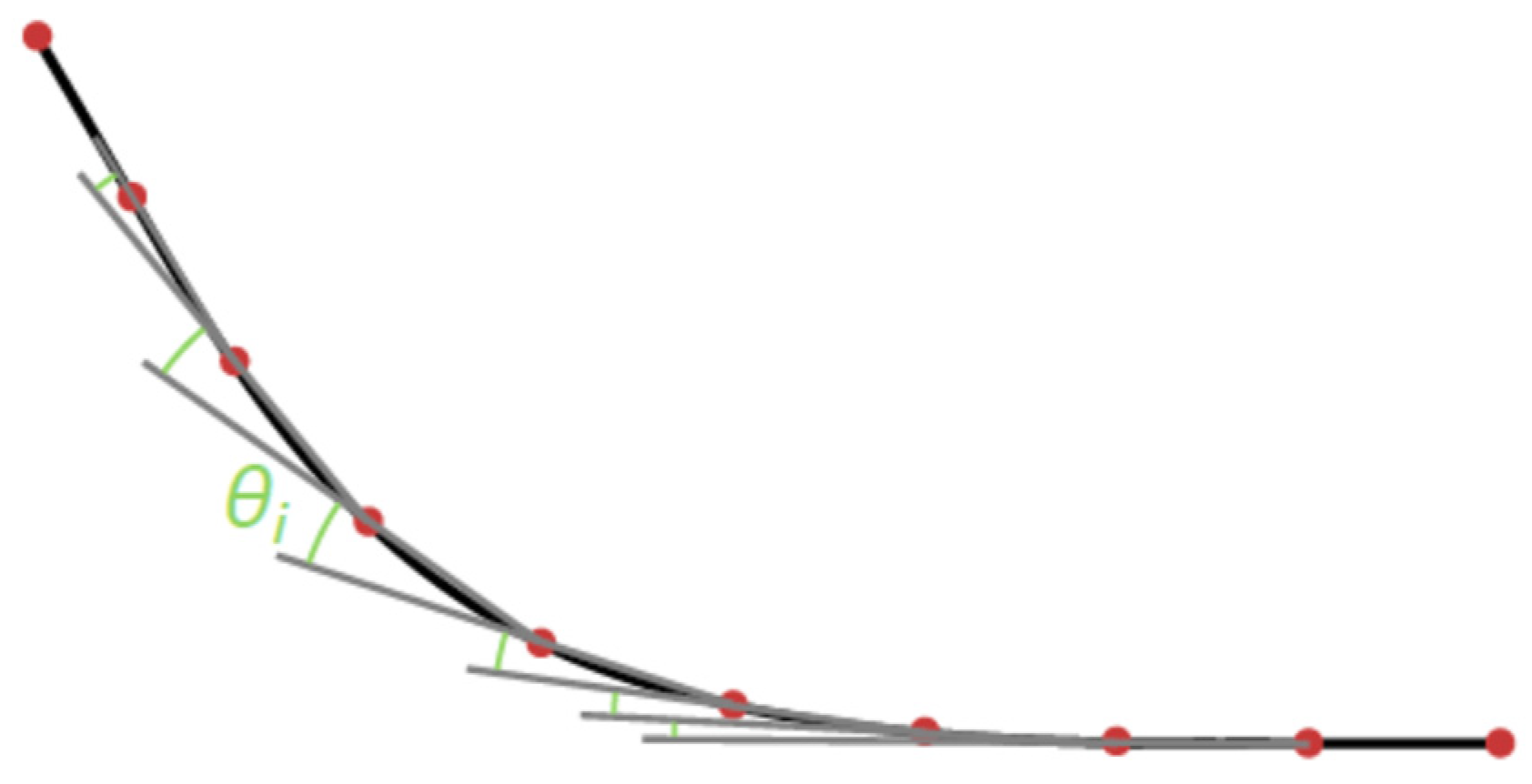
The proposed algorithm was implemented as a global planner in ROS in C++ language so it could be used in the move_base package to navigate a robot. Simulations were made with the help of Gazebo and RViz environments. The results of the proposed algorithm (later denoted as FlFill) were compared with currently commonly used methods in the path planning of mobile robots—A* and Dijkstra. The first criterion for comparing the algorithms was execution time. It also includes the time to call the service in ROS and to get the answer. It is, therefore, slightly higher than the real execution time. The second criterion was the length of the path. The third criterion is the total change in the orientation angle around axis z required to complete a given path. This criterion is computed based on two direction vectors created from three consecutive curve points. The first direction vector is from the first point to the second. The second direction vector is from the second point to the third. Let them denote a = (ax, ay), b = (bx, by). Their scalar product can be expressed in two ways:
From this system of equations then follows:
If the vectors are unit vectors, the equation can be simplified:
The total rotation change is then obtained by counting all partial angles. Figure 8 shows some partial angles marked in green on the example of a simple curve.
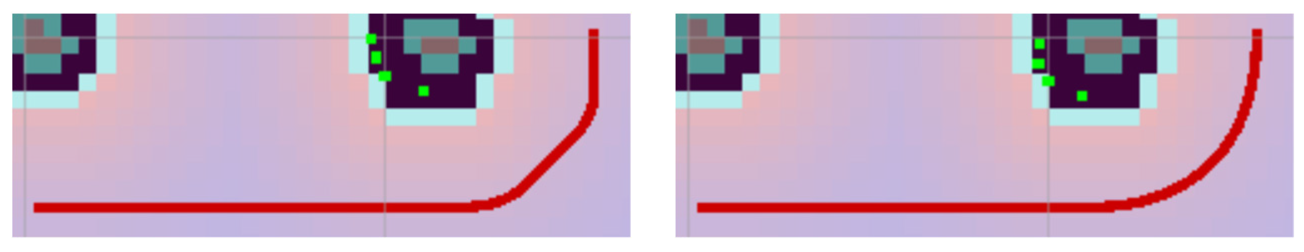
In the case of the Dijkstra and A* algorithms, only some points were used to calculate the overall change in the rotation angle. Generally, only every fifth point was used, and every tenth point was used for the last two environments. The reduction of the analyzed points was proposed because the points generated by these algorithms were close to each other and were not lying on the lines, which was observable, especially in the case of algorithm A* (Figure 9). This fact caused a high value of the sum of changes in the rotation angle. In the case of the proposed algorithm (based on wavefront), such a problem did not occur because the points from the generated path are located on lines. In the case of the proposed algorithm, even a tenfold increase in the number of generated points caused only a tiny change in the sum of angles.
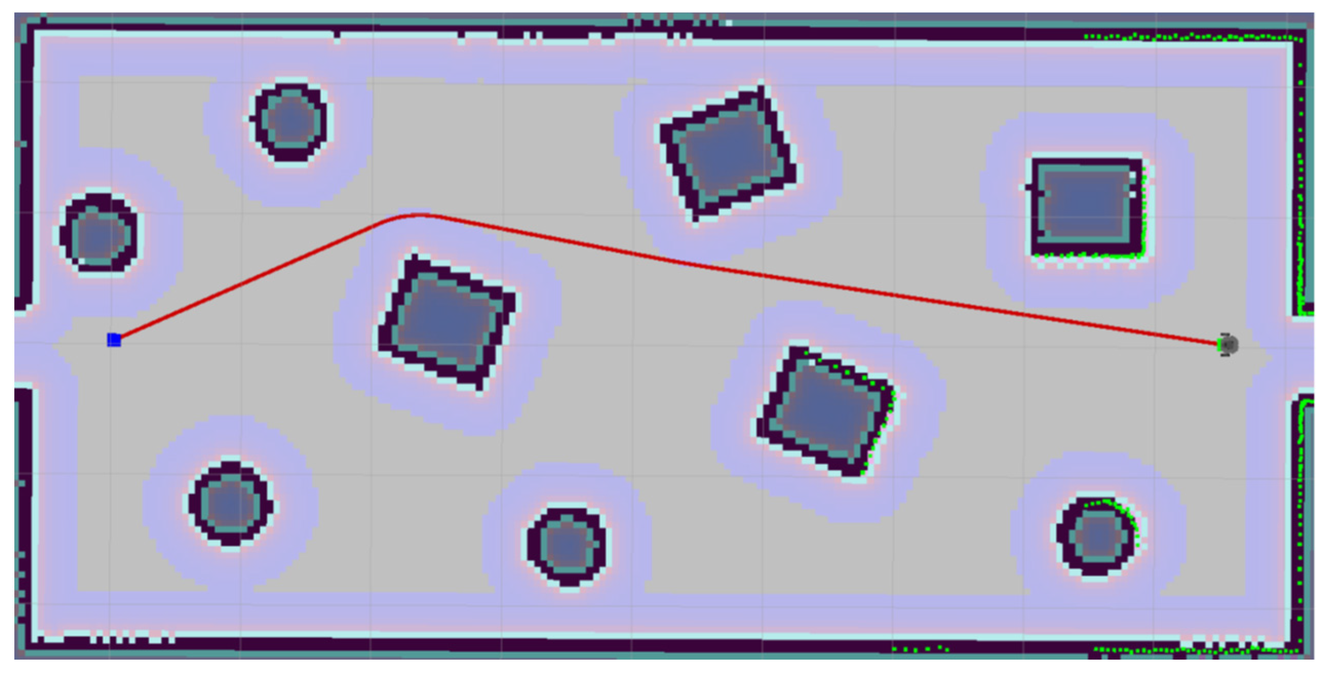
Five pairs of starting and goal points were tested in each modeled environment. The algorithms were run five times for each point pair to determine the average execution time. That means 25 times for every environment. The real execution times and the duration of its parts are also stated for the proposed (wavefront-based) algorithm. For this purpose, in most cases, the time representing the median of the five runs was selected, and the average was calculated from them. The path length and the sum of the rotation angle changes were also calculated as the average result of five pairs of points for a given environment. The map resolution used was 0.05 m. The cthold parameter was set to 3 for all algorithms so that all three algorithms maintain a similar distance from obstacles. First, a smaller environment was tested for three different obstacle densities. The low-density environment can be seen in Figure 10. The size of the map is approximately 200 × 95 cells.
The execution time was the lowest for the proposed method (Table 1). Although the proposed approach did not reach the shortest path, it was characterized by a relatively low sum of changes in rotation.
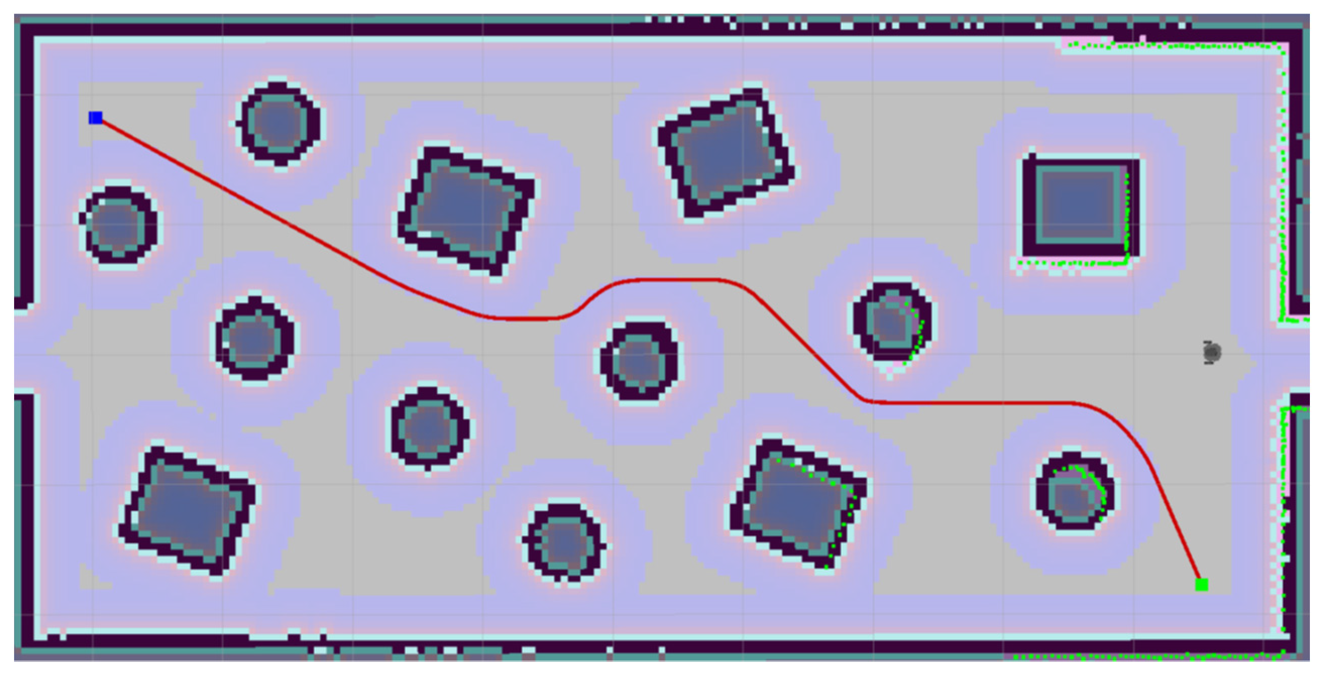
Four additional obstacles were added to the medium obstacle density environment (Figure 11). The results show (Table 2) that the proposed algorithm is again the best concerning the robot’s sum of rotations. However, at the time of the computation, it is only second behind A*, and in terms of path length, it is also second after Dijkstra’s algorithm.
Thirteen obstacles were placed to make the high-density environment (Figure 12). In this environment, the advantages of the proposed algorithm have already manifested themselves significantly (Table 3). Its calculation time is the best, the path length is the second best, and it is the best to minimize the robot’s rotation along the path. This tested environment is relatively small, so the calculation of all algorithms is very fast. It means a relatively large portion of the execution time is communicating with the service. Therefore, the average values of the calculation time may not be considered a significant characteristic. The average time it took to call for service was 3.336 ms for the proposed algorithm and this environment. The following table (Table 4) shows the average execution times for the individual phases of the proposed algorithm. These are averages for all three obstacle densities because the calculation times were comparable. The most computationally demanding part was filling the matrix (map) with values, which took more than half of the execution time.
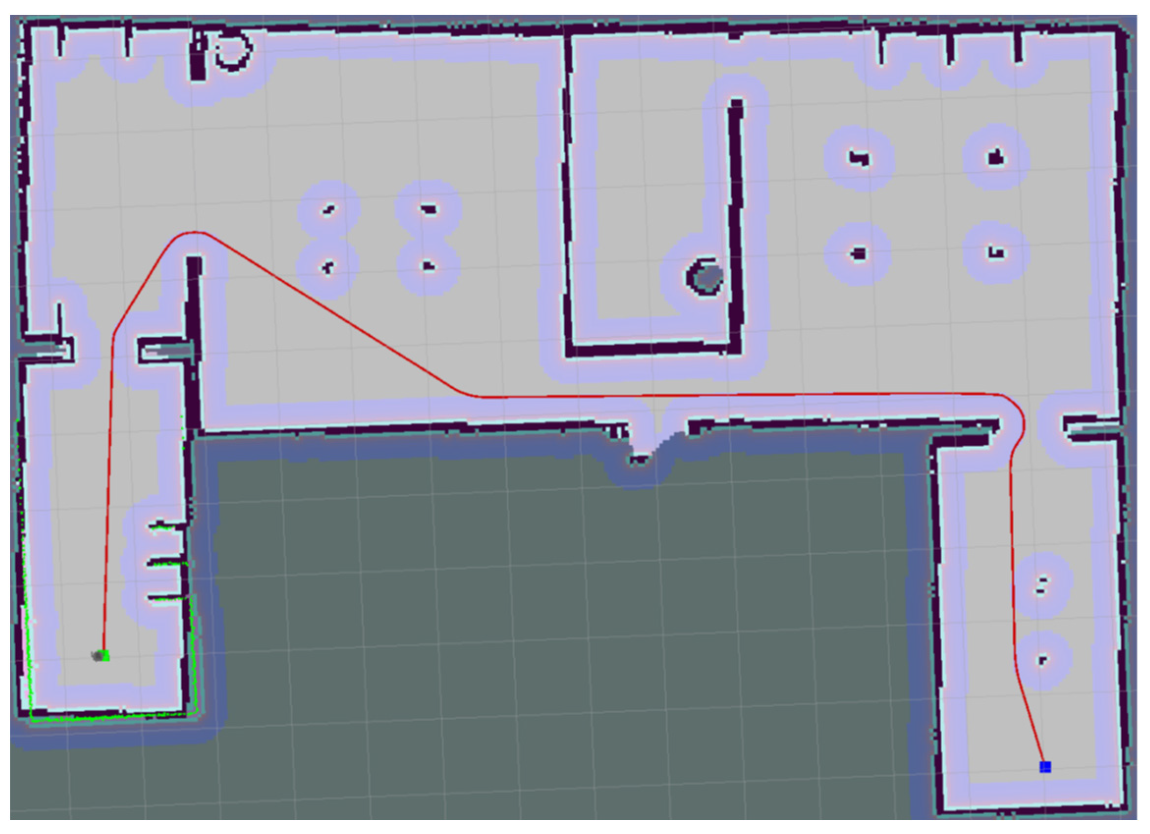
The other environments tested were two larger environments. The size of the first one is approximately 290 × 180 cells; for example, it can represent one floor of the house (Figure 13).
In this environment (Table 5), the proposed algorithm also reached the lowest sum of the rotation angle. As in previous environments, Dijkstra’s algorithm found the shortest average path. Algorithm A* achieved the shortest average execution time.
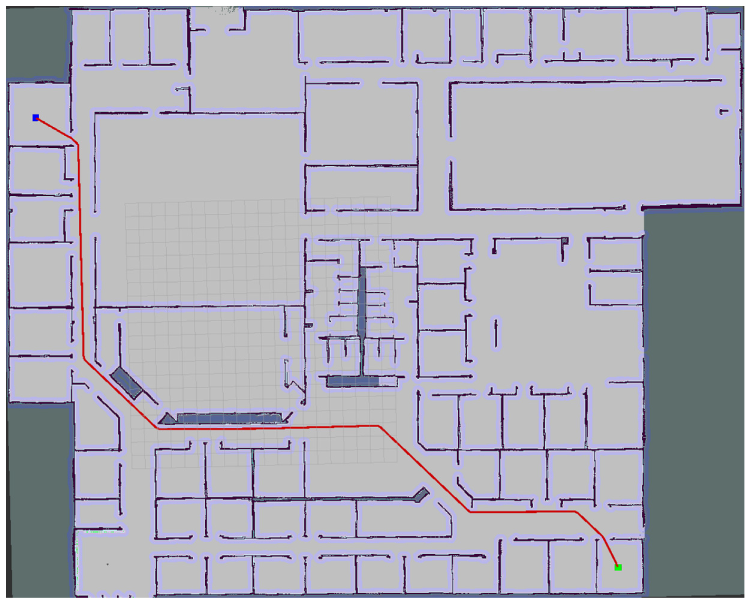
The largest portion of the execution time, in this case, more than 80 percent, was again taken up by the evaluation of the map cells, as can be seen in Table 6. The second largest portion was taken by finding the path on the evaluated matrix. The other phases needed significantly less time to be completed. The last environment is the largest, with a size of approximately 1100 × 900 cells. It is a mapped Willow Garage robotic laboratory (Figure 14) containing many interconnected rooms of various sizes.
As in the previous environment, the shortest execution time was achieved by the A* algorithm. Dijkstra’s algorithm found the shortest average path, and the proposed algorithm again achieved the lowest overall change in the rotation angle (Table 7). As we can observe, the portion of time (Table 8) required to evaluate the cells of the map grows with the increasing size of the map. It is also because several phases of the algorithm do not depend directly on the size of the environment. In the case of the largest environment, the filling of the map represented over 95 percent of the total execution time.
Since all three algorithms provide a specific advantage (Dijkstra’s, the shortest path; A*, the fastest calculation; FlFill, the smallest sum of rotational changes), a comparison of the algorithms’ multi-criteria was made. Let the execution time be denoted by t, the length of the path l, and the total change of the angle of rotation θ. First, these parameters are multiplied by the constants kt, kl, and kθ (Table 9) so that their effect on the resulting value is balanced on average. They are then multiplied by the weights wt, wl, and wθ, which express the selected preference of the properties of individual algorithms. The criterion function for the evaluation of algorithms can be formulated as follows:
Two larger environments were evaluated in this way. Constants with indices containing h belong to the house environment, and if they have the index w, they belong to the Willow Garage environment.
Due to the fact mentioned above, with the evaluation of the total rotation angle in the Dijkstra and A* algorithms, the weight of the parameter θ was chosen to be 0.6. The path length was first preferred for the remaining two parameters, so the parameters wt = 1 and wl = 1.2 were chosen. Results can be seen in Table 10 In the second part, the execution time was preferred over the path length, and therefore the parameters wt = 1.2 and wl = 1 were chosen (Table 11). In the results, both types of environments are compared. The value of the function for the house environment is denoted as fh, for the Willow Garage environment as fw, and for their sum as f.
4. Discussion
We can conclude that all three algorithms achieved similar overall results, but each excelled in a different area. The A* algorithm achieved the lowest execution time in many scenarios. Still, its path length was higher, and it needed a higher sum of changes in rotation angle to execute the resulting path. Dijkstra’s algorithm was computationally more expensive. It achieved the shortest path length and needed a higher sum of changes in the robot’s rotation angle. The proposed algorithm FlFill achieved low execution time in smaller environments (higher in more complex environments); the resulting path length was in the middle of the three algorithms, but the sum of changes in the rotation angle was the lowest in all scenarios.
One interesting area where the proposed algorithm could be useful is the navigation of visually impaired people, mainly because of its property of keeping low total change in the orientation angle around the z-axis. It would be beneficial in all cases, emphasizing the smoothness of the generated trajectory or low changes in the rotation angle.
5. Conclusions
This research presents the proposed algorithm using the wavefront algorithm and modifying its generated path using B-spline curves. This algorithm was compared with the A* and Dijkstra algorithms and achieved similar results. However, it excels in smaller action interventions and the execution of a given path, which can be very important for some mobile robot applications. The algorithm can be further improved using dual wavefront propagation during the map-filling phase. This phase took up most of the computational time. The result should be a shorter computational time and, thus, an improvement in this feature of the algorithm. In future work, we would also like to conduct experiments with a robot in a real environment. That should verify the dynamic properties of the presented algorithm and could lead to some adjustments and improvements.
Moreover, the generated path can be easily modified according to the real kinematics (or dynamics) of the robot. It is possible by the designed and proven way of reducing redundant waypoints in the path as well as by using B-spline curves for smoothing the path. By simple parameterization, it is possible to modify the generated path concerning the limitations of the robot and, at the same time, minimize costs according to the required criteria.
Author Contributions
Conceptualization, M.P. and F.D.; methodology, M.P.; software, M.P.; validation, M.P., D.M. and T.M.; formal analysis, M.R.; investigation, D.M.; resources, F.D.; data curation, M.P.; writing—original draft preparation, F.D.; writing—review and editing, T.M.; visualization, M.P.; supervision, F.D.; project administration, F.D.; funding acquisition, F.D. All authors have read and agreed to the published version of the manuscript.
Funding
This research was supported by projects KEGA 028STU-4/2022, ESA AO/1-10044/19/NL/SC, and UAVLIFE (“Research and development of the applicability of autonomous flying vehicles in the fight against the pandemic caused by COVID-19”, Project no. 313011ATR9, co-financed by the European Regional Development Fund.).
Conflicts of Interest
The authors declare no conflict of interest.
References
- Durrant-Whyte, H.; Bailey, T. Simultaneous localization and mapping: Part I. IEEE Robot. Autom. Mag. 2006, 13, 99–110. [Google Scholar] [CrossRef]
- Thrun, S. Simultaneous Localization and Mapping. In Robotics and Cognitive Approaches to Spatial Mapping; Jefferies, M.E., Yeap, W.K., Eds.; Springer: Berlin/Heidelberg, Germany, 2008; pp. 13–41. [Google Scholar] [CrossRef]
- Ünver Akmandor, N.; Padır, T. A 3D Reactive Navigation Algorithm for Mobile Robots by Using Tentacle-Based Sampling. arXiv 2020, arXiv:2001.09199. [Google Scholar]
- Aggarwal, S.; Kumar, N. Path planning techniques for unmanned aerial vehicles: A review, solutions, and challenges. Comput. Commun. 2020, 149, 270–299. [Google Scholar] [CrossRef]
- Ayawli, B.B.K.; Mei, X.; Shen, M.; Appiah, A.Y.; Kyeremeh, F. Mobile Robot Path Planning in Dynamic Environment Using Voronoi Diagram and Computation Geometry Technique. IEEE Access 2019, 7, 86026–86040. [Google Scholar] [CrossRef]
- Teleweck, P.E.; Chandrasekaran, B. Path planning algorithms and their use in robotic navigation systems. In Journal of Physics: Conference Series; IOP Publishing: Bristol, UK, 2019; Volume 1207, p. 012018. [Google Scholar]
- Wolek, A.; Woolsey, C.A. Model-based path planning. In Sensing and Control for Autonomous Vehicles: Applications to Land, Water and Air Vehicles; Fossen, T., Pettersen, K., Nijmeijer, H., Eds.; Springer: Cham, Switzerland, 2017; pp. 183–206. [Google Scholar]
- Siegwart, R.; Nourbakhsh, I.R. Introduction to Autonomous Mobile Robots; Bradford Company: Holland, MI, USA, 2004. [Google Scholar]
- Nakajima, K.; Premachandra, C.; Kato, K. 3D environment mapping and self-position estimation by a small flying robot mounted with a movable ultrasonic range sensor. J. Electr. Syst. Inf. Technol. 2017, 4, 289–298. [Google Scholar] [CrossRef]
- Sakurama, K.; Sugie, T. Generalized Coordination of Multi-robot Systems. Found. Trends® Syst. Control. 2021, 9, 1–170. [Google Scholar] [CrossRef]
- Kuric, I.; Bulej, V.; Saga, M.; Pokorny, P. Development of simulation software for mobile robot path planning within multilayer map system based on metric and topological maps. Int. J. Adv. Robot. Syst. 2017, 14, 1729881417743029. [Google Scholar] [CrossRef]
- Murphy, R.R. Introduction to AI Robotics, 1st ed.; MIT Press: Cambridge, MA, USA, 2000. [Google Scholar]
- Bräunl, T. Embedded Robotics: Mobile Robot Design and Applications with Embedded Systems, 2nd ed.; Springer: Berlin/Heidelberg, Germany, 2006. [Google Scholar]
- Nemec, D.; Gregor, M.; Bubeníková, E.; Hruboš, M.; Pirnik, R. Improving the Hybrid A* method for a non-holonomic wheeled robot. Int. J. Adv. Robot. Syst. 2019, 16, 1729881419826857. [Google Scholar] [CrossRef]
- Ferguson, D.; Stentz, A. Using interpolation to improve path planning: The Field D* algorithm. J. Field Robot. 2006, 23, 79–101. [Google Scholar] [CrossRef]
- Choset, H.; Lynch, K.; Hutchinson, S.; Kantor, G.; Burgard, W.; Kavraki, L.; Thrun, S. Principles of Robot Motion: Theory, Algorithms, and Implementations; MIT Press: Cambridge, MA, USA, 2005. [Google Scholar]
- Saranya, C.; Unnikrishnan, M.; Ali, S.A.; Sheela, D.S.; Lalithambika, V.R. Terrain based D∗ algorithm for path planning. IFAC-PapersOnLine 2016, 49, 178–182. [Google Scholar] [CrossRef]
- Zhang, B.; Li, G.; Zheng, Q.; Bai, X.; Ding, Y.; Khan, A. Path planning for wheeled mobile robot in partially known uneven terrain. Sensors 2022, 22, 5217. [Google Scholar] [CrossRef] [PubMed]
- Ichter, B.; Schmerling, E.; Lee, T.W.E.; Faust, A. Learned Critical Probabilistic Roadmaps for Robotic Motion Planning. In Proceedings of the 2020 IEEE International Conference on Robotics and Automation (ICRA), Paris, France, 31 May–31 August 2020; pp. 9535–9541. [Google Scholar] [CrossRef]
- Karur, K.; Sharma, N.; Dharmatti, C.; Siegel, J.E. A Survey of Path Planning Algorithms for Mobile Robots. Vehicles 2021, 3, 448–468. [Google Scholar] [CrossRef]
- Nagib, G.; Gharieb, W. Path planning for a mobile robot using genetic algorithms. In Proceedings of the International Conference on Electrical, Electronic and Computer Engineering, Cairo, Egypt, 5–7 September 2004; pp. 185–189. [Google Scholar] [CrossRef]
- LaValle, S.M. Planning Algorithms; Cambridge University Press: Cambridge, MA, USA, 2006. [Google Scholar]
- Lin, H.Y.; Huang, Y.C. Collaborative Complete Coverage and Path Planning for Multi-Robot Exploration. Sensors 2021, 21, 3709. [Google Scholar] [CrossRef] [PubMed]
- Dung, V.T.; Tjahjowidodo, T. A direct method to solve optimal knots of B-spline curves: An application for non-uniform B-spline curves fitting. PLoS ONE 2017, 12, e0173857. [Google Scholar] [CrossRef]
- Piegl, L.; Tiller, W. The NURBS Book, 2nd ed.; Springer: Berlin/Heidelberg, Germany, 1997. [Google Scholar]
- Looi, C.Z.; Ng, D.W.K. A Study on the Effect of Parameters for ROS Motion Planer and Navigation System for Indoor Robot. Int. J. Electr. Comput. Eng. Res. 2021, 1, 29–36. [Google Scholar] [CrossRef]
- Amanatides, J.; Woo, A. A Fast Voxel Traversal Algorithm for Ray Tracing. In Eurographics; Department of Computer Science, University of Toronto: Toronto, ON, Canada, 1987; Volume 87. [Google Scholar]
Figure 1.
Inflation of obstacles in the ROS environment by a safe distance and impact on the planned path of the robot.
Figure 1.
Inflation of obstacles in the ROS environment by a safe distance and impact on the planned path of the robot.

Figure 2.
Example of removing two redundant points (right) at the top left and bottom right on the original path (left).
Figure 2.
Example of removing two redundant points (right) at the top left and bottom right on the original path (left).

Figure 3.
Example of adding control points around a waypoint (original curve on the (left), two control points added on the (right)).
Figure 3.
Example of adding control points around a waypoint (original curve on the (left), two control points added on the (right)).

Figure 4.
The proposed algorithm.

Figure 5.
(Top left)—path found by wavefront algorithm, (top right)—path without redundant points, (bottom left)—addition of control points, (bottom right)—result path.
Figure 5.
(Top left)—path found by wavefront algorithm, (top right)—path without redundant points, (bottom left)—addition of control points, (bottom right)—result path.

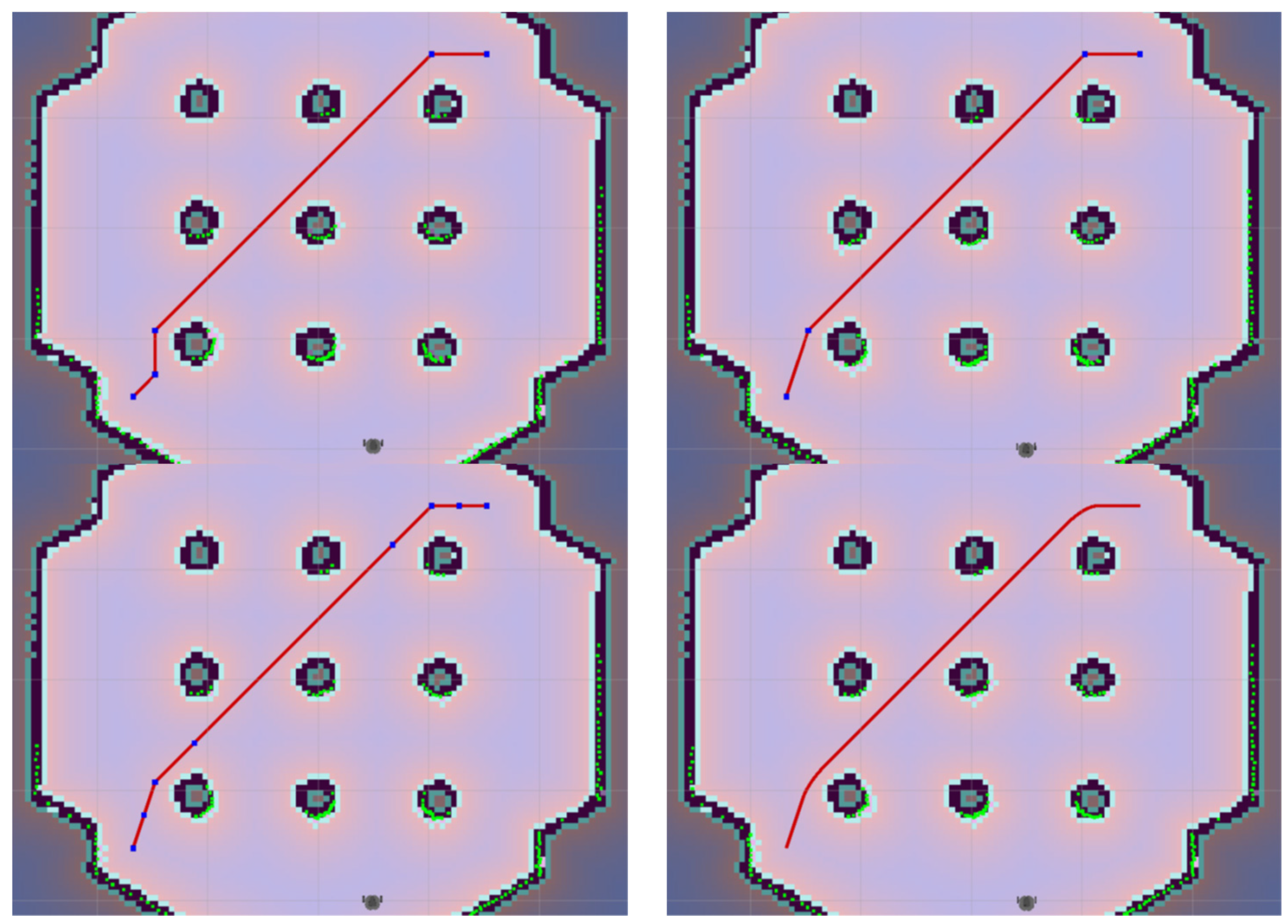
Figure 6.
Influence of the parameter cthold—on the (left) with the value 200 and on the (right) with the value 128.
Figure 6.
Influence of the parameter cthold—on the (left) with the value 200 and on the (right) with the value 128.

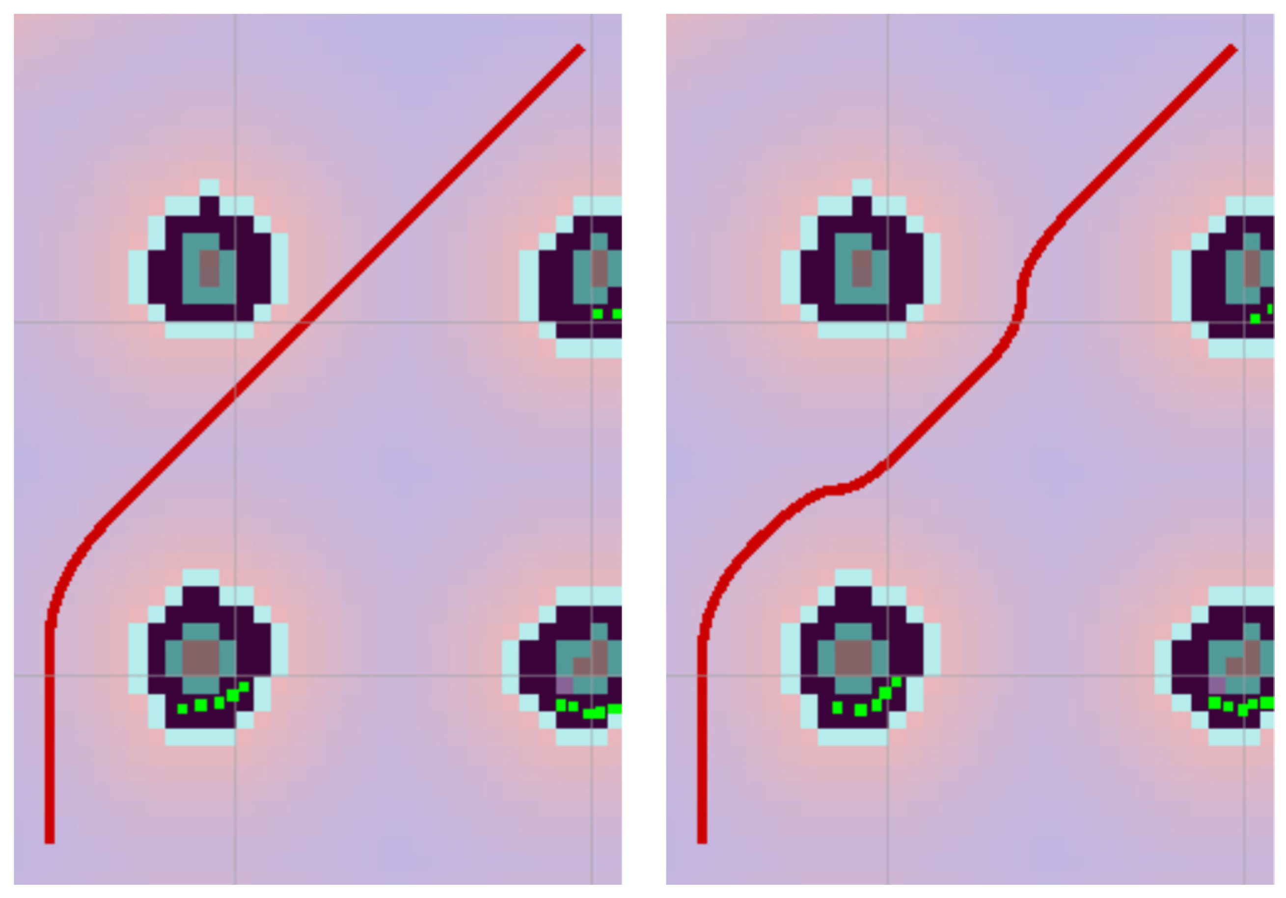
Figure 7.
Influence of the cpthold parameter on the shape of the B-spline curve (value 0.25 on the (left) and value 0.5 on the (right)).
Figure 7.
Influence of the cpthold parameter on the shape of the B-spline curve (value 0.25 on the (left) and value 0.5 on the (right)).

Figure 8.
Rotational angles are derived from points on the robot’s path.

Figure 9.
Oscillation of the path generated by the A* algorithm.

Figure 10.
An environment with low obstacle density.

Figure 11.
An environment with medium obstacle density.

Figure 12.
An environment with a high density of obstacles.

Figure 13.
Medium-sized environment (house).

Figure 14.
Large environment—Willow Garage.


Table 1.
Comparison of results of individual algorithms for the environment with low obstacle density.
Table 1.
Comparison of results of individual algorithms for the environment with low obstacle density.
| Algorithm | Execution Time [ms] | Path Length [m] | ∑ θi [rad] |
|---|---|---|---|
| FlFill | 5.0684 | 9.3293 | 1.2678 |
| Dijkstra | 5.2612 | 9.1902 | 2.6219 |
| A* | 6.2873 | 9.7801 | 5.3037 |
Table 2.
Comparison of results of individual algorithms for the environment with medium obstacle density.
Table 2.
Comparison of results of individual algorithms for the environment with medium obstacle density.
| Algorithm | Execution Time [ms] | Path Length [m] | ∑ θi [rad] |
|---|---|---|---|
| FlFill | 5.5888 | 9.4812 | 2.3788 |
| Dijkstra | 6.9644 | 9.2192 | 3.7174 |
| A* | 3.9387 | 9.8144 | 7.7095 |
Table 3.
Comparison of results of individual algorithms for the environment with high obstacle density.
Table 3.
Comparison of results of individual algorithms for the environment with high obstacle density.
| Algorithm | Execution Time [ms] | Path Length [m] | ∑ θi [rad] |
|---|---|---|---|
| FlFill | 4.4656 | 9.7948 | 4.9412 |
| Dijkstra | 7.2702 | 9.4945 | 5.0040 |
| A* | 6.5048 | 9.8728 | 9.0146 |
Table 4.
Execution times of individual phases of the FlFill algorithm.
| Phase of Algorithm | Execution Time [ms] | Portion [%] |
|---|---|---|
| Initialization | 0.3345 | 19.86 |
| Filling the map | 0.8711 | 51.72 |
| Finding a path | 0.3101 | 18.42 |
| Removing redundant points | 0.0503 | 2.98 |
| Creating control points | 0.0111 | 0.66 |
| Generating curve points | 0.1071 | 6.36 |
| ∑ | 1.6841 | 100 |
Table 5.
Comparison of results of individual algorithms for medium-sized environments.
| Algorithm | Execution Time [ms] | Path Length [m] | ∑ θi [rad] |
|---|---|---|---|
| FlFill | 10.5711 | 19.2237 | 5.5476 |
| Dijkstra | 9.6750 | 19.0329 | 6.5439 |
| A* | 7.3334 | 19.5487 | 11.5688 |
Table 6.
Execution times of individual phases of the FlFill algorithm for a medium-sized environment.
Table 6.
Execution times of individual phases of the FlFill algorithm for a medium-sized environment.
| Phase of Algorithm | Execution Time [ms] | Portion [%] |
|---|---|---|
| Initialization | 0.1868 | 2.46 |
| Filling the map | 6.1534 | 80.98 |
| Finding a path | 0.8188 | 10.78 |
| Removing redundant points | 0.1672 | 2.20 |
| Creating control points | 0.0208 | 0.27 |
| Generating curve points | 0.2516 | 3.31 |
| ∑ | 7.5986 | 100 |
Table 7.
Comparison of results of individual algorithms for the large environment (Willow Garage).
| Algorithm | Execution Time [ms] | Path Length [m] | ∑ θi [rad] |
|---|---|---|---|
| FlFill | 99.6838 | 59.5385 | 7.7551 |
| Dijkstra | 107.0439 | 57.7588 | 10.2174 |
| A* | 41.6553 | 60.2191 | 26.9868 |
Table 8.
Execution times of individual phases of the FlFill algorithm for a large environment.
| Phase of Algorithm | Execution Time [ms] | Portion [%] |
|---|---|---|
| Initialization | 1.0310 | 1.09 |
| Filling the map | 90.1950 | 95.44 |
| Finding a path | 2.2764 | 2.41 |
| Removing redundant points | 0.1698 | 0.18 |
| Creating control points | 0.0308 | 0.03 |
| Generating curve points | 0.7972 | 0.84 |
| ∑ | 94.5002 | 100 |
Table 9.
Parameters for individual environments.
| Parameter | Value | Parameter | Value |
|---|---|---|---|
| kth | 1.0878 | ktw | 0.1208 |
| klh | 0.519 | klw | 0.169 |
| kθh | 0.9787 | kθw | 0.6673 |
Table 10.
Comparison results for wt = 1 and wl = 1.2.
| Algorithm | wtktht | wlklhl | Wθkθhθ | wtktwt | wlklwl | wθkθwθ | fh | fw | f |
|---|---|---|---|---|---|---|---|---|---|
| FlFill | 11.5 | 11.97 | 3.26 | 12.04 | 12.07 | 3.11 | 26.73 | 27.22 | 53.951 |
| Dijkstra | 10.52 | 11.85 | 3.84 | 12.93 | 11.71 | 4.09 | 26.22 | 28.74 | 54.956 |
| A* | 7.98 | 12.17 | 6.79 | 5.03 | 12.21 | 10.81 | 26.95 | 28.05 | 54.995 |
Table 11.
Comparison results for wt = 1.2 and wl = 1.
| Algorithm | wtktht | wlklhl | wθkθhθ | wtktwt | wlklwl | wθkθwθ | fh | fw | f |
|---|---|---|---|---|---|---|---|---|---|
| FlFill | 13.80 | 9.98 | 3.26 | 14.45 | 10.06 | 3.10 | 27.03 | 27.62 | 54.651 |
| Dijkstra | 12.63 | 9.88 | 3.84 | 15.52 | 9.76 | 4.09 | 26.35 | 29.37 | 55.719 |
| A* | 9.57 | 10.15 | 6.79 | 6.04 | 10.18 | 10.80 | 26.51 | 27.02 | 53.532 |
Disclaimer/Publisher’s Note: The statements, opinions and data contained in all publications are solely those of the individual author(s) and contributor(s) and not of MDPI and/or the editor(s). MDPI and/or the editor(s) disclaim responsibility for any injury to people or property resulting from any ideas, methods, instructions or products referred to in the content. |
© 2023 by the authors. Licensee MDPI, Basel, Switzerland. This article is an open access article distributed under the terms and conditions of the Creative Commons Attribution (CC BY) license (https://creativecommons.org/licenses/by/4.0/).
Share and Cite
MDPI and ACS Style
Psotka, M.; Duchoň, F.; Roman, M.; Michal, T.; Michal, D. Global Path Planning Method Based on a Modification of the Wavefront Algorithm for Ground Mobile Robots. Robotics 2023, 12, 25. https://doi.org/10.3390/robotics12010025
AMA Style
Psotka M, Duchoň F, Roman M, Michal T, Michal D. Global Path Planning Method Based on a Modification of the Wavefront Algorithm for Ground Mobile Robots. Robotics. 2023; 12(1):25. https://doi.org/10.3390/robotics12010025
Chicago/Turabian StylePsotka, Martin, František Duchoň, Mykhailyshyn Roman, Tölgyessy Michal, and Dobiš Michal. 2023. "Global Path Planning Method Based on a Modification of the Wavefront Algorithm for Ground Mobile Robots" Robotics 12, no. 1: 25. https://doi.org/10.3390/robotics12010025
Note that from the first issue of 2016, this journal uses article numbers instead of page numbers. See further details here.