Virtual UR5 Robot for Online Learning of Inverse Kinematics and Independent Joint Control Validated with FSM Position Control ^†

Abstract

Virtual remote laboratories have already been successfully implemented in educational centers for practical learning of mechatronics and robotic systems. This article presents the development of a virtual articulated UR-type robot, designed as an educational tool that is suitable for programming and evaluating both the inverse kinematics control of the robot and the independent control of the robot joints. The 3D model of the virtual robot was developed in the Blender V2.79 software and uses the Modbus TCP industrial communication protocol for the communication to an external controller implemented in CoDeSys V3.5 software. The developed system allows the students to generate and test their own control algorithm for the robot joints with the visualization of the achieved performance in 3D and real time. Tailored control systems can be compared on the virtual robot. In this study, a novel technique for the joint position control based on an FSM is proposed and verified with the virtual UR5 robots to prove that the developed system is a suitable platform to teach and learn the inverse kinematics control and independent joint control of the UR5 robotic arm.

1. Introduction

Information and communication technologies are valuable tools that favor teaching and learning. Today, engineering education applies different tools such as computer simulation and virtual reality through remote access and video calls for online learning. Virtual laboratories (VL) have been developed at educational centers as educational platforms for training engineering students in industrial processes and technological systems. The application of VL allows to develop technical skills, specifically in mechatronics, robotics, and automation systems, which integrate actuators, sensors, industrial control systems, and networks.

The VL introduces users to the concept of cyber-physical systems (CPSs), which are composed of physical systems with their computational models [1]. CPSs are capable of connecting networked devices of different information and communication technology systems, virtualizing different laboratories [2]. CPS is a key technology for the application of Industry 4.0. To develop a robotics VL, dynamic models of sensors, actuators, and mechanisms are required, in addition to a control system that can compensate for the response of the real mechatronic system. The graphic model of the robot needs to be designed and animated in 3D. The VL has similar features to the digital twin. Digital twins can be implemented with 3D models, numerical simulation, and a virtual reality interface [3,4]. Learning kits that incorporate digital twins are practical tools for acquiring understanding and practice of engineering concepts [5,6].

Today, there are different types of virtual laboratories oriented in different engineering specialties such as control systems, process monitoring, robotics, mechatronics, and automation [7,8]. Research and development centers develop robotic unit platforms incorporating 3D models, designed in CAD software. Universities in China have created robotics virtual laboratories in Unity 3D software [9] as teaching platforms. VLs have been developed for different robot models, such as a 6DOF manipulator anthropomorphic industrial robot, to perform autonomous object manipulation tasks in virtual environments [10]. The UR-10 robot has also been developed in augmented virtual reality [11]. Dynamics and control systems can also be taught in interactive virtual labs using mechatronic models [12].

This work is an enhancement of a previous article [13] presenting the design, implementation, and control of a virtual UR5-type articulated robot for its use as an e-learning platform. The 3D model of the UR5 robot was simulated and animated in the Blender V2.79 software. Codesys V3.5 software was used to develop and implement the control system in a Hardware in the loop (HIL) simulation scheme. The robot simulator communicates with the robot controller via the Modbus TCP industrial network protocol. The developed system is oriented toward the teaching and learning of the kinematic control of robots and the real-time control of the articulated joints. Users develop skills in robot inverse kinematics and in the control of the robot actuators, which are key topics in robot design and control courses. The challenge for the student is to design and implement the lower control levels of the robot in an external controller, that is, the control of speed and position of the joints, and the direct and inverse kinematic control. This document describes, in Section 2, the methods used for the virtual robot design and, in Section 3, the methods and control techniques applied to the virtual robot. Section 4 shows and discusses the results obtained from the system. Lastly, the conclusions are presented in Section 5.

2. Methods for Virtual Robot Design

In this section, the software for virtual robotics laboratory development, the methods for 3D modeling of the UR5 robot with Blender, and kinematics analysis of the UR robot are presented.

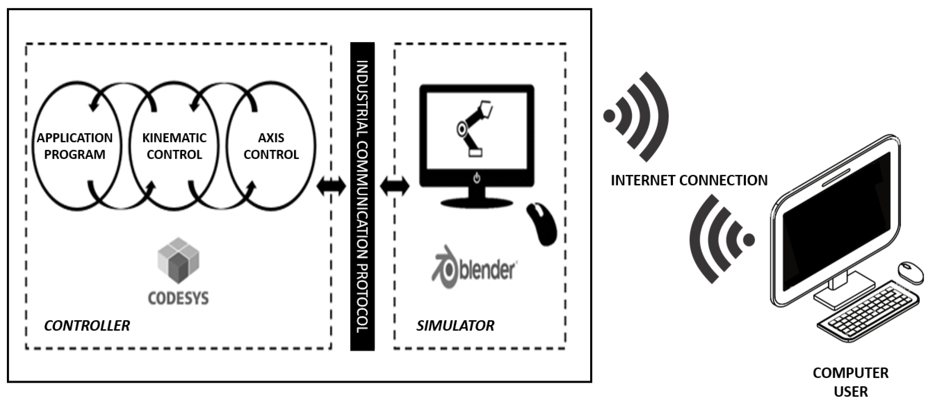
2.1. Virtual Robotics Laboratory

Currently, robot manufacturers provide virtual 3D models of the robot, which are integrated into the development and monitoring software in order to assist the programming and operation of the robot for training purposes. Virtual robots are tools that help learning automation in workplaces and educational institutions. The development of this project of a virtual UR5 robot uses Blender V2.79 © software for the animation of the 3D model and Codesys V3.5 © software for the control of the system, integrating two required levels of robot control: joint control and inverse kinematic control. Applications developed using Blender and Codesys communicate through a Modbus TCP industrial network protocol. Additionally, Radmin V1.2 © software is used to provide remote access to the system. Figure 1 shows the general scheme of the system.

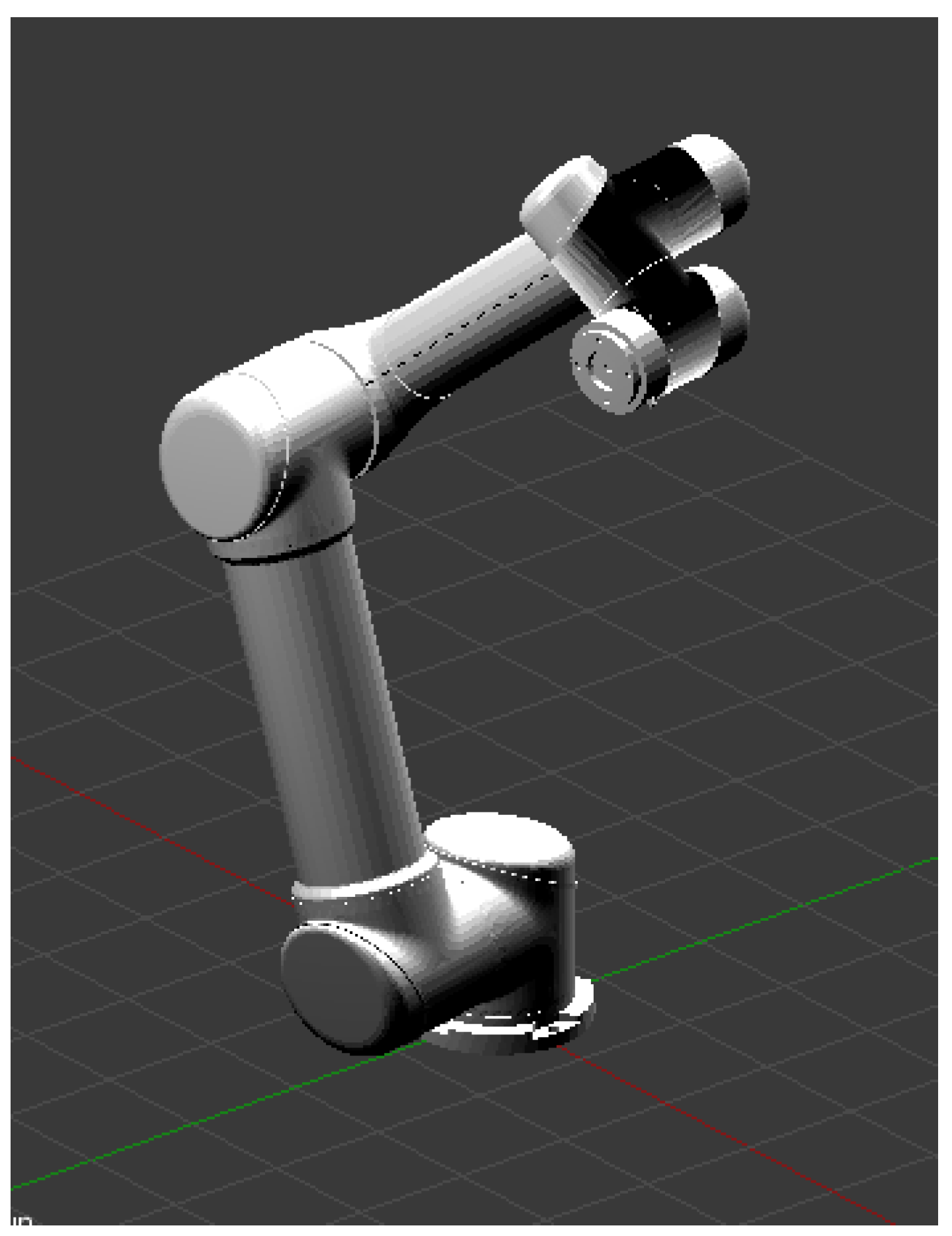
2.2. 3D Modeling of the UR5 Robot with Blender

To make the 3D model of the UR5 robot, Blender software was used as an animation and simulation platform for the project because it is freely accessible and its work environment allows industrial network communication. Currently there are different CAD software companies that develop simulations and 3D models: Unity, CATIA, ANSYS, Autodesk Inventors, and SolidWorks [14,15,16]. Figure 2 shows the 3D model developed in Blender.

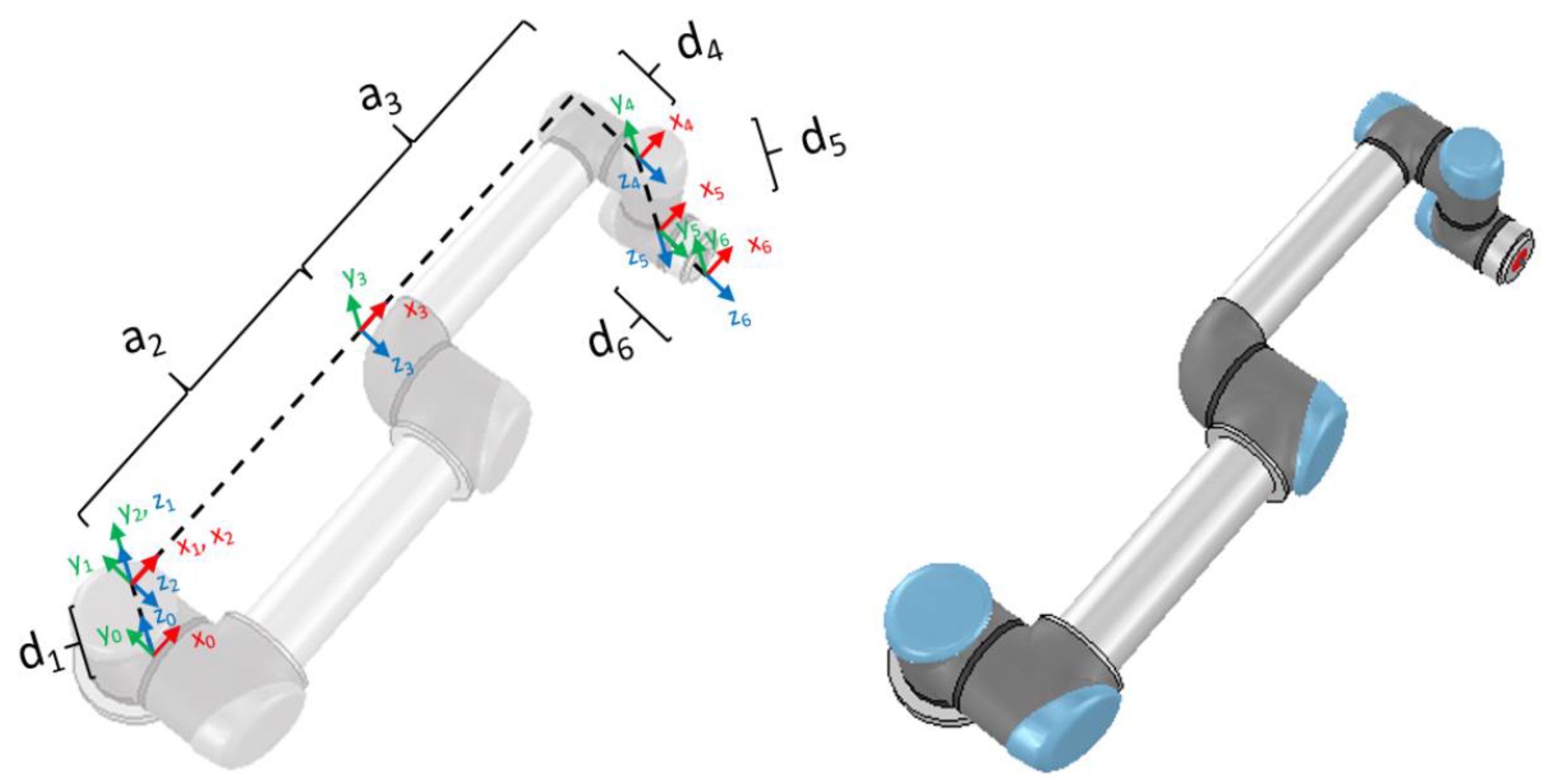
2.3. Kinematics of the UR Robot

The direct kinematics of the UR5 robot can be obtained through the geometry and spatial location of each one of the links that make up the system, while the inverse kinematics can be achieved through the determination of the joint variables as a function of the position and end effector orientation. The UR5 robot kinematic model is necessary for the numerical simulation and control of the UR5 virtual robot. This work studies the kinematics of the robot using the Denavit–Hartenberg (D–H) method. Figure 3 shows the joint frames [17] and parameter indications to define the homogeneous transform matrices [18].

The UR5 robot is an articulated arm model with six degrees of freedom via rotary joints. The parameters calculated through the reference frames are represented in

Table 1. D–H parameters. Adapted with permission from ref. [13]. Copyright 2021 IEEE.

i	${\mathit{\alpha }}_{\mathit{i}}$	${\mathit{a}}_{\mathit{i}}$	${\mathit{d}}_{\mathit{i}}$	${\mathit{\theta }}_{\mathit{i}}$
1	$\frac{\pi }{2}$	0	$L_1$	${\theta }_1$
2	0	$a_2$	0	${\theta }_2$
3	0	$a_3$	0	${\theta }_3$
4	$\frac{\pi }{2}$	0	$L_4$	${\theta }_4$
5	$-\frac{\pi }{2}$	0	$L_5$	${\theta }_5$
6	0	0	$L_6$	${\theta }_6$

, according to the D–H algorithm, where i is the joint number, α_i is the angle measured between consecutive x-axes, a_i is the distance measured along the x-axis between z-axes, d_i is the distance measured along the z-axis, and θ_i is the angle measured around the z-axis.

The general homogeneous transform matrix of the D–H methodology is given by Equation (1). The direct kinematics solution is obtained by multiplying the six homogeneous transform matrices as shown in Equation (2). The resultant matrix describes the position and orientation of the end effector with respect to the base of the robot.

$${}_{}{}^{i-1}T{}_i=\left[\begin{array}{cccc}\cos {\theta }_i& -\sin {\theta }_i·\cos a_i& \sin {\theta }_i·\sin a_i& a_i·\cos {\theta }_i\\ \sin {\theta }_i& \cos {\theta }_i·\cos a_i& \cos {\theta }_i·\sin a_i& a_i·\sin {\theta }_i\\ \begin{array}{c}0\\ 0\end{array}& \begin{array}{c}\sin a_i\\ 0\end{array}& \begin{array}{c}\cos a_i\\ 0\end{array}& \begin{array}{c}{d}_i\\ 1\end{array}\end{array}\right].$$

(1)

$${}_{}{}^{0}T{}_6={}_{}{}^{0}T{}_1·{}_{}{}^{1}T{}_2·{}_{}{}^{2}T{}_3·{}_{}{}^{3}T{}_4·{}_{}{}^{4}T{}_5·{}_{}{}^{5}T{}_6=\left[\begin{array}{cccc}{r}_{11}& r_{12}& r_{13}& p_x\\ r_{21}& r_{22}& r_{23}& p_y\\ \begin{array}{c}{r}_{31}\\ 0\end{array}& \begin{array}{c}{r}_{32}\\ 0\end{array}& \begin{array}{c}{r}_{33}\\ 0\end{array}& \begin{array}{c}{p}_z\\ 1\end{array}\end{array}\right].$$

(2)

This work uses a kinematic solution previously presented in [17,19]; the complete derivation can be found in these references. By simplifying the calculation of the matrix in Equation (2), it is possible to obtain the equations for the orientation (Equations (3) through (11)) and position (Equations (12) through (14)) elements.

$$r_{11}=c_1{c}_{234}{c}_5{c}_6+c_6{s}_1{s}_5-c_1{s}_{234}{s}_6.$$

(3)

$$r_{12}=-c_1{c}_{234}{c}_5{c}_6-s_1{s}_5{s}_6-c_1{c}_6{s}_{234}.$$

(4)

$$r_{13}=-c_1{c}_{234}{s}_5+c_5{s}_1.$$

(5)

$$r_{21}=c_{234}{c}_5{c}_6{s}_1-c_1{c}_6{s}_5-s_1{s}_{234}{s}_6.$$

(6)

$$r_{22}=-c_{234}{c}_5{s}_1{c}_6+c_5{s}_5{s}_6-c_6{s}_1{s}_{234}.$$

(7)

$$r_{23}=-c_{234}{s}_1{s}_5-c_1{c}_5.$$

(8)

$$r_{31}=c_5{c}_6{s}_{234}+c_{234}{s}_6.$$

(9)

$$r_{32}=-c_5{c}_6{s}_{234}+c_{234}{c}_6.$$

(10)

$$r_{33}=-s_{234}{s}_5.$$

(11)

$$p_x=-c_1{c}_{234}{s}_5{d}_6+c_5{s}_1{d}_6+c_1{s}_{234}{d}_5+s_1{d}_4+c_1{c}_{23}{a}_3+c_1{c}_2{a}_2.$$

(12)

$$p_y=-c_{234}{s}_1{s}_5{d}_6-c_1{c}_5{d}_6+s_1{s}_{234}{d}_5-c_1{d}_4+c_{23}{s}_1{a}_3+c_2{s}_1{a}_2.$$

(13)

$$p_z=-s_{234}{s}_5{d}_6-c_{234}{d}_5+s_{23}{a}_3+s_2{a}_2+d_1.$$

(14)

The solution of the inverse kinematics of the UR5 robot is obtained from the previous equations. The joint angles from the end effector position and orientation are given by the following equations:

$$A_1=p_x-d_6{r}_{13}.$$

(15)

$$B_1=d_6{r}_{23}-p_y.$$

(16)

$$K_c=p_x{c}_1+p_y{s}_1+c_{234}{s}_5{d}_6-s_{234}{d}_5.$$

(17)

$$K_s=p_z-d_1+c_{234}{d}_5+s_{234}{s}_5{d}_6.$$

(18)

$${\theta }_1=a\tan 2\left(A_1,B_1\right)\pm a\tan 2\left(\sqrt{A_1^2+B_1^2-d_4^2,d_4}\right).$$

(19)

$${\theta }_2=a\tan 2\left(K_s,K_c\right)-a\tan 2\left(a_3{s}_3,a_3{c}_3+a_2\right).$$

(20)

$${\theta }_3=\pm a\tan 2\left(s_2,s_3\right).$$

(21)

$${\theta }_4={\theta }_{234}-{\theta }_2-{\theta }_3.$$

(22)

$${\theta }_5=\pm a\tan 2\left(s_5,c_5\right).$$

(23)

$${\theta }_6=a\tan 2\left(s_6,c_6\right).$$

(24)

3. Methods for Virtual Robot Control

In this section, several speed control schemes are presented for DC motors: speed servo control, PID joint position control, and finite state machine for joint position control, in addition to a comparison of the methods.

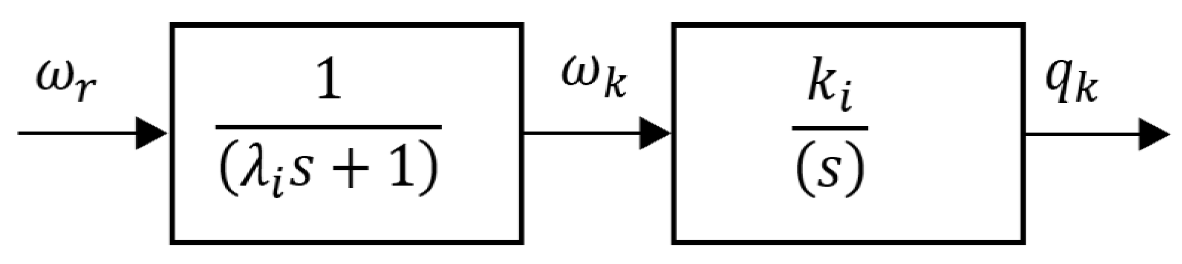
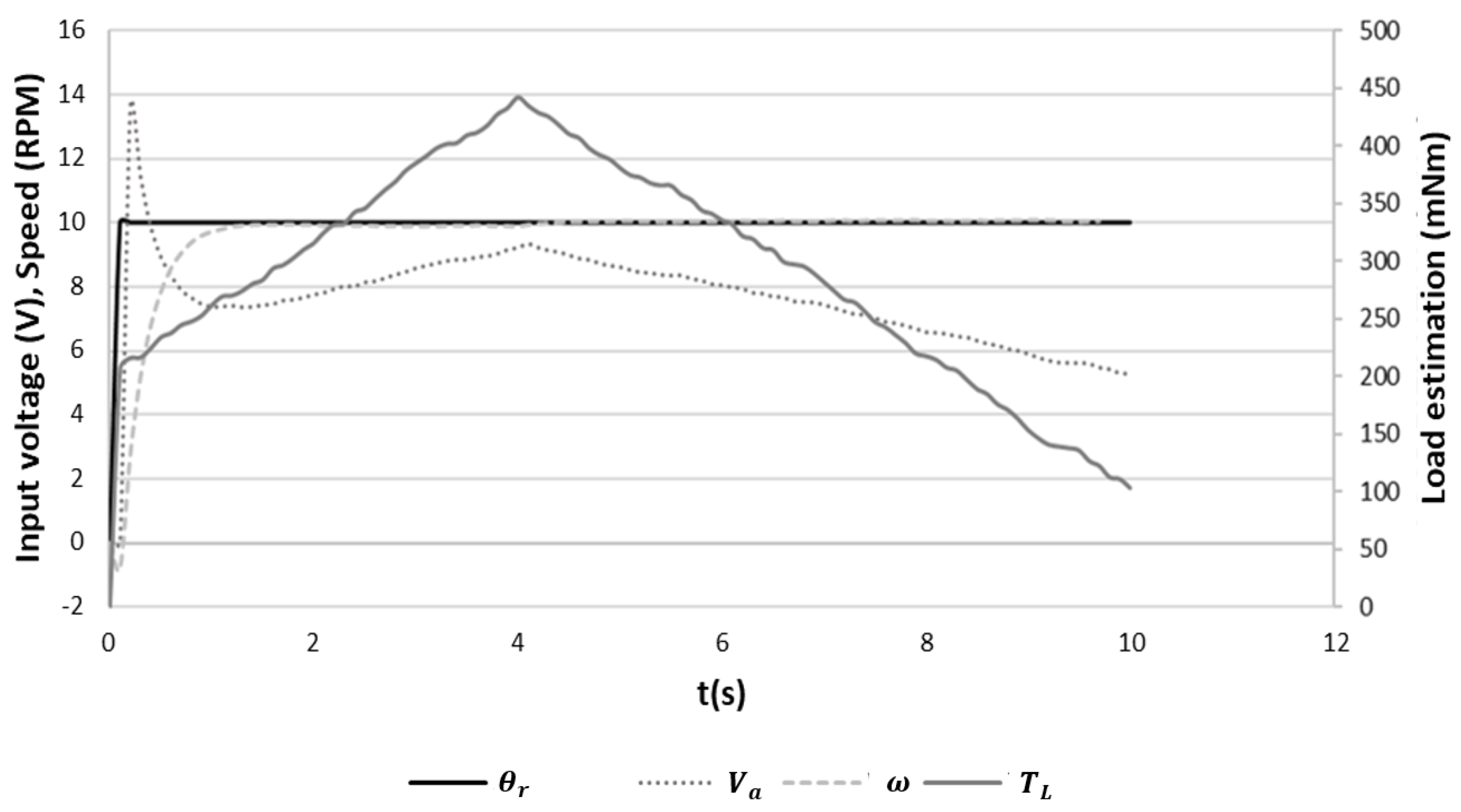
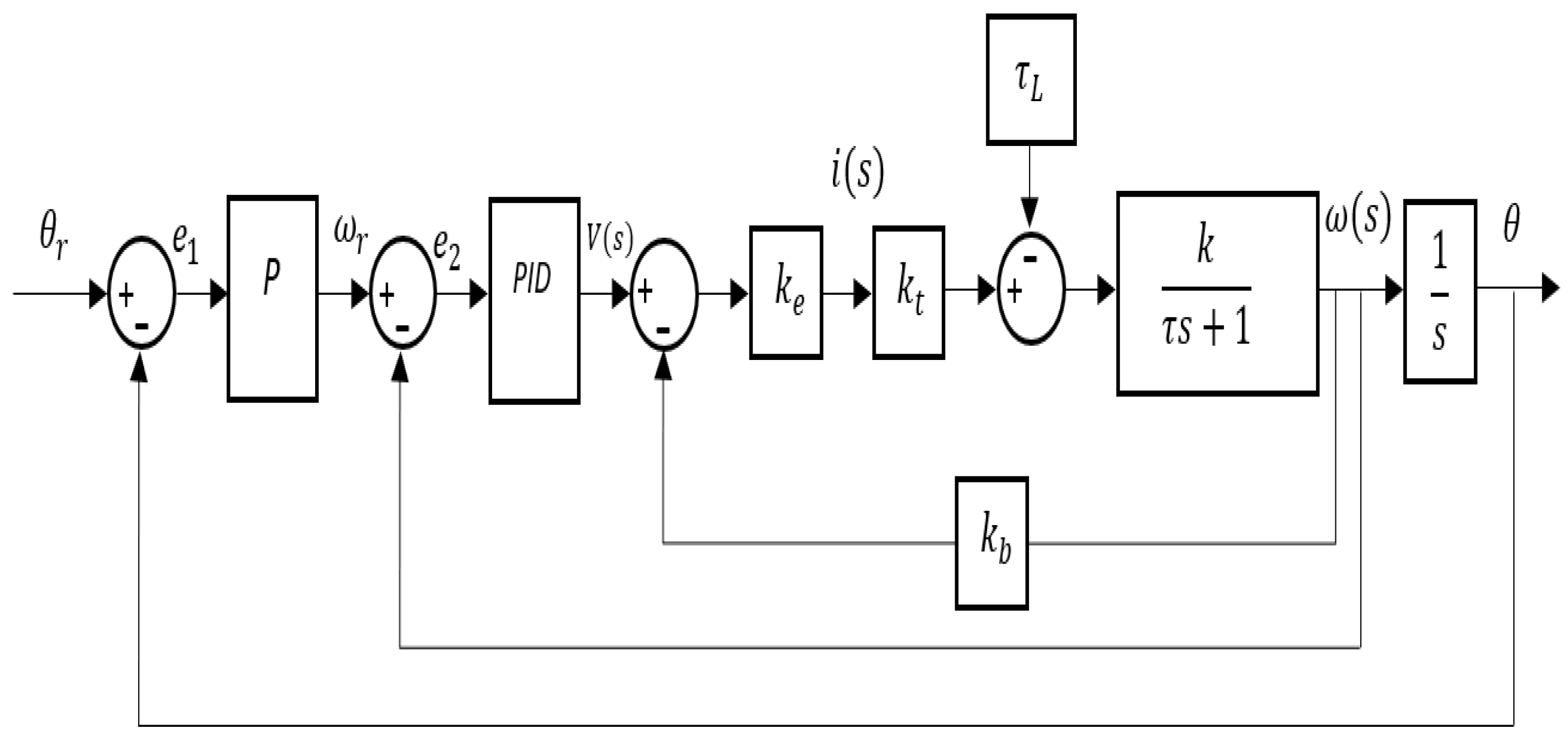
3.1. Speed Servo Control of DC Motors

The DC motor has an angular positioning system that is commonly controlled through PID control algorithms to optimize its operation [20]. Since the motor speed is integrated in the mechanical process, only a proportional controller is needed to control the position of a DC motor shaft. DC motors can be used as actuators to produce the rotational movement of the joints of the robotic arm. The dynamic response of six DC motors has to be considered to represent the six articulations or the UR5 robot. Individual actuator models are suitable for designing the independent control of the joints as a practical and robust approach. The assumption of high-ratio gearboxes (i.e., 100:1) connecting the motor shaft to the mechanical load implies the consideration of negligible dynamic perturbations and allows the use of simplified actuator models. The mathematical model of the servo-controlled DC motor can be stated in two parts: the first-order dynamics of the angular speed, and the integration of the achieved speed to obtain the angular position, as shown in Figure 4. This model can be discretized by the Euler backward difference method (EBD) and used as a basis for modeling of the complete robot [21].

The angular position with respect to the speed reference is given by

$$G_i\left(s\right)=\frac{1}{\left({\lambda }_{i}s+1\right)}\times \frac{k_i}{s}=\frac{k_i}{\left({\lambda }_i{s}^2+s\right)}.$$

(25)

However, the model components can be implemented separately. The speed servo control dynamics or first model subsystem in Figure 4 can be expressed in discrete time as

$${\omega }_k=\alpha \times {\omega }_{k-1}+\left(1-\alpha \right)\times {\omega }_r.$$

(26)

The second model subsystem or speed integrator to calculate angular position is discretized as

$$q_k=\alpha \times q_{k-1}+T_s\times k_i\times {\omega }_k.$$

(27)

where ${\omega }_k$ is the current angular speed, ${\omega }_r$ is the speed reference, $q_k$ is the current position, $k_i$ is the integrator gain, $T_s$ is the sampling period, and $\alpha$ is a parameter defined as a function of the servo-control time constant ${\lambda }_i$ and $T_s$, given by

$$\alpha =\frac{{\lambda }_i}{{\lambda }_i+T_s}.$$

(28)

The equations presented in this subsection are sufficient to simulate the closed-loop dynamical response of the robot joints; under this scenario, the actuators are servomotors, and this configuration can be used to test different position controllers.

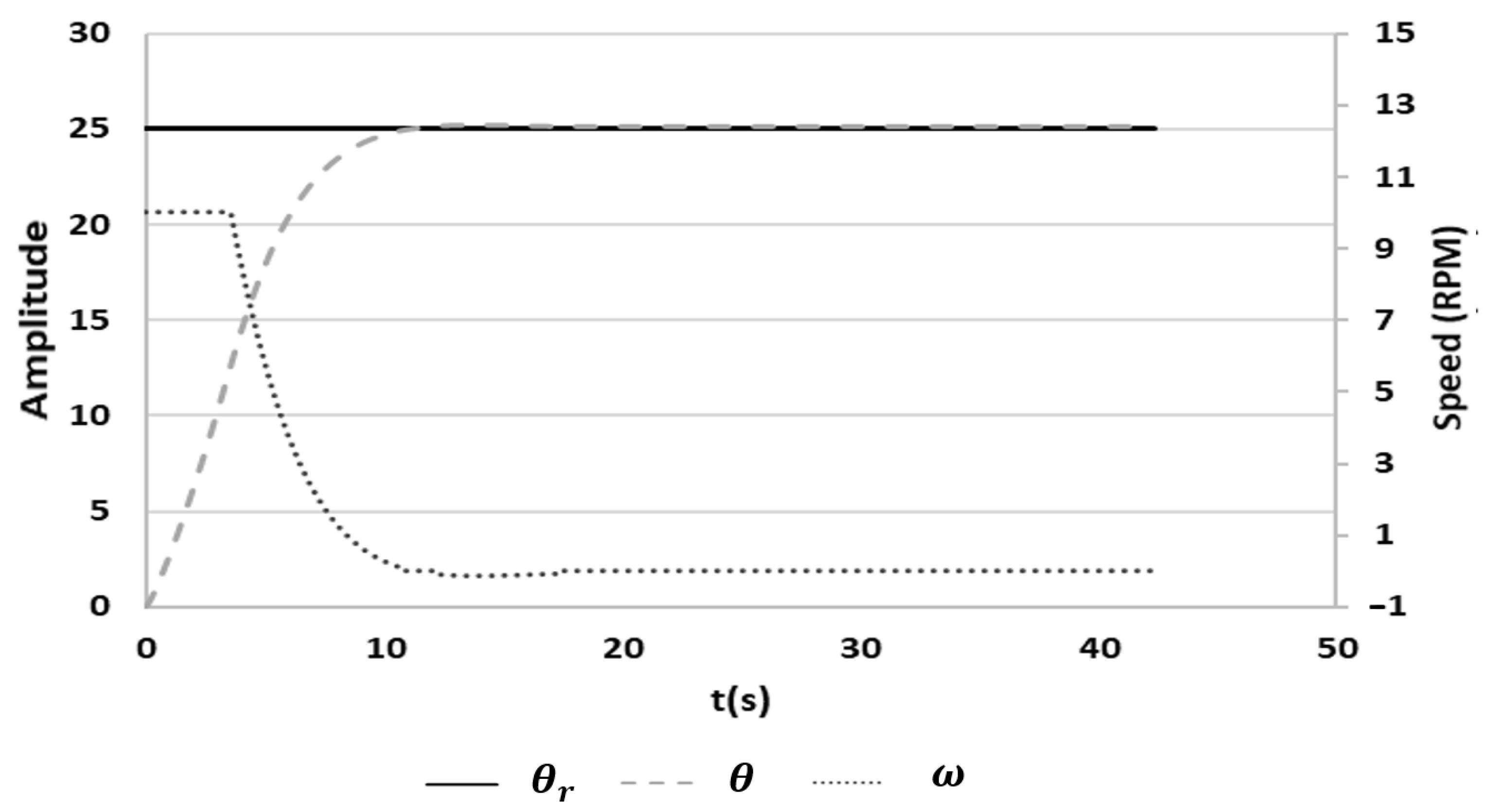
3.2. PID Joint Position Control

A more detailed modeling and control of the speed of the robot joints can be defined if the joint actuators are considered to be DC motors that require the implementation of speed controllers. The proportional–integral–derivative (PID) controller is a widely used control technique that is employed for the regulatory feedback control of dynamic systems [22]. PID is expressed in terms of the error signal I and has a proportional gain ($k_P$), an integral gain ($k_I$), and a derivative gain ($k_D$). The ideal continuous PID controller has the following form:

$$u\left(t\right)=k_P·e\left(t\right)+k_I\int e\left(t\right)·dt+k_D·\frac{de\left(t\right)}{dt}.$$

(29)

For simplification, Equation (29) can be converted to Equation (30) considering a unique common controller gain:

$$u\left(s\right)=e\left(s\right)·k_C\left[1+\frac{1}{T_i·s}+T_d·s\right],$$

(30)

with the following tuning parameters: controller gain $k_C$, integral time constant $T_i$, and derivative time constant $T_d$.

Equation (30) can be rearranged as Equation (31) to ease the discretization of the control law:

$$T_i·s·u\left(s\right)=k_C\left(T_i·T_d·s^2+T_i·s+1\right)·e\left(s\right).$$

(31)

A discrete time representation of Equation (31) can be obtained by applying the EBD method:

$$T_i·\left(\frac{u_K-u_{K-1}}{T}\right)=k_C·\left[T_i·T_d\left(\frac{e_K-2e_{K-1}+e_{K-2}}{T^2}\right)+T_i·\left(\frac{e_K-e_{K-1}}{T}\right)+e_K\right].$$

(32)

For producing a discrete trapezoidal integration form, the last error term can be substituted by an average of two error samples in Equation (33) and expressed as Equation (34):

$$e_K=\frac{e_K+e_{K-1}}{2},$$

(33)

$$T_i·\left(\frac{u_K-u_{K-1}}{T}\right)=k_C·\left[T_i·T_d\left(\frac{e_K-2e_{K-1}+e_{K-2}}{T^2}\right)+T_i·\left(\frac{e_K-e_{K-1}}{T}\right)+\frac{e_K+e_{K-1}}{2}\right].$$

(34)

Therefore, the expression for the control law in discrete time is

$$u_K=u_{K-1}+k_C·\left[\left(e_K-e_{K-1}\right)+\frac{T}{T_I}·\left(\frac{e_K+e_{K-1}}{2}\right)+\frac{T_d}{T}·\left(e_K-2e_{K-1}+e_{K-2}\right)\right].$$

(35)

The internal model control (IMC) principle can be used to tune up the PIDs. The IMC-PID tuning criterion generates a robust controller for a fast and non-oscillating response despite the variations of the motor parameters [23,24].

The controller parameters for the DC motor model are as follows:

$$k_c=K_d=\frac{1}{K_m}·\frac{{\tau }_m}{{\tau }_{LC}},$$

(36)

$$T_i=\frac{{\tau }_m+{\tau }_{LC}}{2},$$

(37)

$$T_d=k_C\frac{\left({\tau }_{L_{ek}}-{\tau }_{L_{ek}-1}\right)}{2}$$

(38)

where ${\tau }_m$ is the mechanical time constant, ${\tau }_L$ is the load torque, ${\tau }_{LC}$ is the desired closed-loop time constant, $K_m$ is the model gain, ${\tau }_{L\_ek}$ is the current load torque, and ${\tau }_{Lek-1}$ is the previous current load.

As can be seen in Figure 5, the joint angular speed is controlled under a reference change and with a non-negligible continuous small variation of the load. In this closed-loop control system response, when the estimated load torque changes, the derivative term compensates for the load torque increase or decrease while the motor speed is kept steady at the desired speed.

The motor angular speed can be controlled by an internal loop with an IMC-PID controller, while the motor angular position is controlled by an external loop with a proportional controller. Figure 6 shows the complete cascade P-PID control strategy. In this control scheme, ${\theta }_r$ and ${\omega }_r$ are the reference signals for the external and internal controllers, respectively, where $e_1$ = ${\theta }_{r–}$− $\theta$ and $e_2$= ${\omega }_{r–}$− $\omega$. The error $e_1$ enters the P controller block that controls the position by adjusting the speed of the motor; therefore, the P controller outpIt is passed as speed reference ${\omega }_r$. The speed error $e_2$ enters the PID controller block; the output of the PID controller applies a voltage to the DC motor to affect the speed. The DC motors model requires the voltage input to develop a speed ω, which is integrated to give an angular position θ of the DC motor shaft or axis of motion. Additionally, the load torque acts as a disturbance variable that can be directly compensated for by the derivative term of the PID speed controller.

The control law for the position controller is given by Equation (39), considering a proportional gain multiplied by the error difference between two consecutive error samples:

$$u_K=u_{K-1}+k_C\left(e_K-e_{K-1}\right).$$

(39)

Since the control variable (or manipulation) is in integral form, upper and lower limits speed limits need to be set:

$$u_K>{\omega }_{max} then u_K={\omega }_{max},$$

(40)

$$u_K<{\omega }_{min} then u_K={\omega }_{min}.$$

(41)

Figure 7 shows the current position signal using a P controller, with $k_C$= 1, $T_i$= 0.7, and a reference signal of 25 (position set point). The speed changes determined by the controller are observed. The maximum speed is ${\omega }_{MAX}$ = 10 rad/s for one direction, and $-{\omega }_{MAX}$ = −10 rad/s for the other direction. There is a dead band in such a way that the minimum speed is ${\omega }_{MIN}$= 0.1 rad/s for one direction, and $-{\omega }_{MIN}$= −0.1 rad/s for the other direction. The speed transition signal drops gradually, reaching the saturation band. The speed is represented on the secondary axis of the graph.

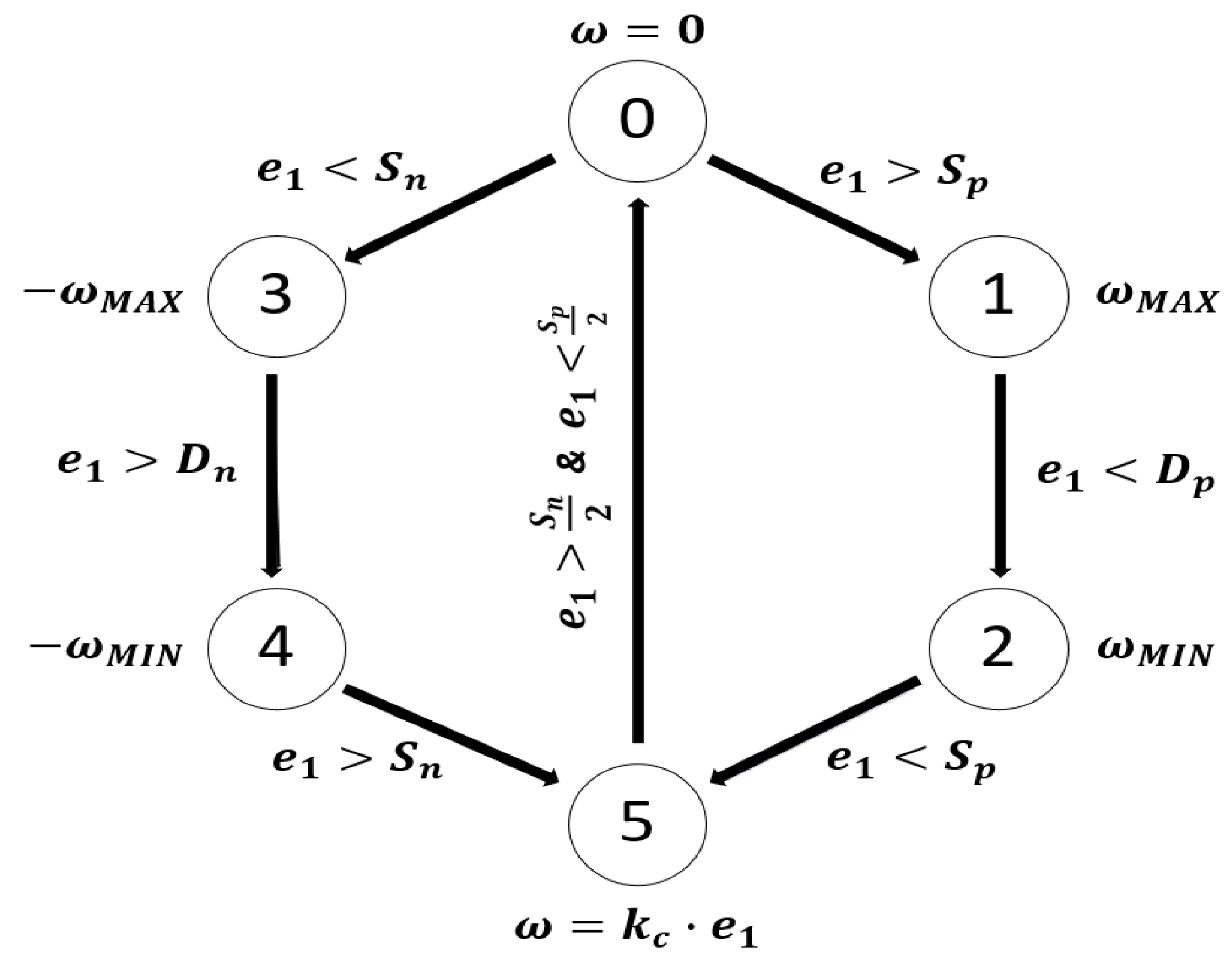
3.3. Finite State Machine for Joint Position Control

The virtual robot is designed for teaching both inverse kinematic control and basic independent joint control strategies such as the one exposed in Section 3.1 and Section 3.2. The virtual robot can also be used for engineering research to propose novel control techniques. In this work, a finite state machine position control strategy is introduced to test the applicability of the virtual robot not only for education but also for research. The finite state machine or finite automaton is defined mathematically with the quintuple G = (X, Σ, δ, $x_0$, $X_m$), where X is the set of states, Σ is the set of symbols of the events, δ represents the events or logical functions for the transitions between states, $x_0$ is the initial state, and $X_m$ is a subset of states. Transition functions are logical conditions for state change (input events or conditions for detecting that the current stage actions are completed, and the system can go to the next state). In the current state, actions are performed (output commands are activated). FSM describes the behavior of the system as a machine with a finite number of states, i.e., through status, events, and actions. FSM is a computational model that can react to the inputs and status of the system, to make transitions from one state to another and generate an output in a period of time [25].

3.3.1. Cascade FSM-IMC-PID for Position and Speed Control

The control strategy where an FSM is used as a position controller is depicted in Figure 8. In the block diagram, the model of the DC motor and the inner and outer loops are represented. The position error signal $e_1$ enters the FSM controller block. The FSM controller output generates a speed reference ${\omega }_r$. The speed error $e_2$ is calculated and sent as the input to the PID controller. The PID controller output is the armature voltage for the DC motor. The DC motor process responds to the voltage input with a speed ω, which is integrated to produce the displacement θ of the DC motor shaft.

For the DC motor position control, the automaton is defined with the following elements: the initial state $x_0$ = 0 corresponds to zero speed output; $X_m$ = {$x_0$} = {0}, i.e., the initial state to ensure that, when the position controller, is activated the system can start a positioning sequence. The states are defined according to the control sequence as X = {$x_0, x_1, x_2, x_3, x_4, x_5$} = {0, 1, 2, 3, 4, 5}, the events are Σ = {${\sigma }_0$, ${\sigma }_1$, ${\sigma }_2$, ${\sigma }_3$, ${\sigma }_4$, ${\sigma }_5$}, and the transition functions are δ = {${\delta }_0$, ${\delta }_1$, ${\delta }_2, {\delta }_3, {\delta }_4, {\delta }_5$}. Figure 9 shows the state diagram of the DC motor position control, where ω is the current speed, e₁ is the position error, $D_n$ is the negative deceleration window, $D_P$ is the positive deceleration window, $S_n$ is the stop negative window, and $S_P$ is the stop positive window. The state diagram has six states that control the position of the motor. The initial state 0 applies zero angular speed, ω = 0. If the position set point is changed, an error is computed. If the error is positive, $e_1$ > $S_P$, the FSM goes to state 1, which generates a constant maximum speed, ${\omega }_{MAX}$, until the error reaches a deceleration window, $e_1$<$D_P$, and the FSM changes to state 2 which applies a minimum speed, ${\omega }_{MIN}$. When the position feedback approaches the desired position, $e_1$ < $S_P$, state 5 is activated and enables a proportional controller, $\omega =k_c\times e_1$, and the transition to state zero happens when $e_1>\frac{S_n}{2}$. State zero applies zero speed and, therefore, stops the motor. If the position setpoint is changed and a negative error is computed, $e_1$<$S_n$, the FSM goes to state 3, which applies a constant maximum negative speed, $-{\omega }_{MAX}$, until the error reaches a deceleration window, $e_1$ > $D_n$; then, the FSM changes to state 4 that applies a minimum speed, $-{\omega }_{MIN}$. When the position feedback approaches the desired position, $e_1$ > $S_n$, it goes to state 5. Finally, the FSM goes to the zero state to set zero speed if $e_1<\frac{S_p}{2}$.

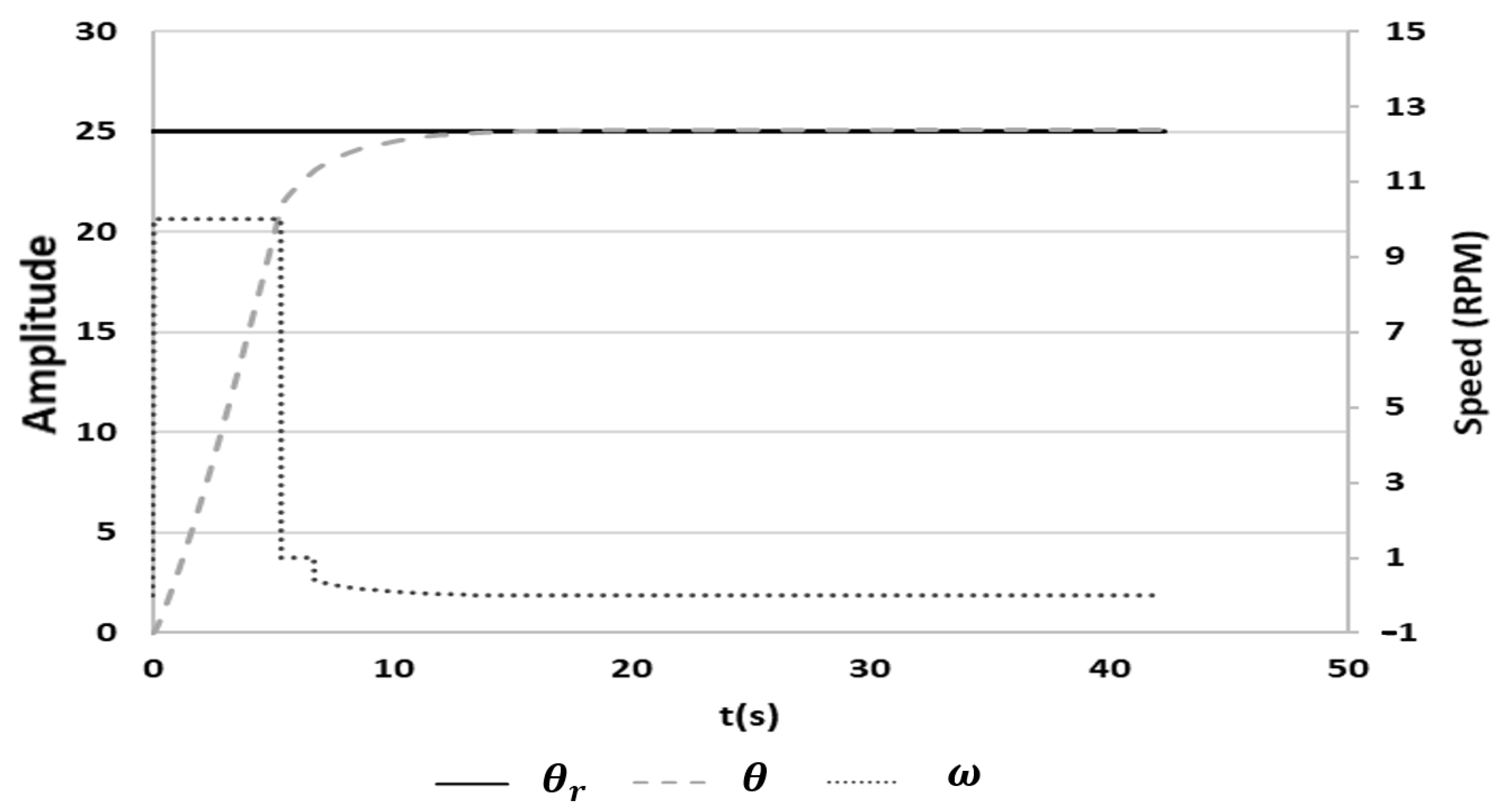
3.3.2. Response of the FSM-IMC-PID Controller

Figure 10 shows the use of an FSM for a controlled position change of the DC motor shaft from a reference of 0 to 25, with the previously mentioned speed limits for the position controller output. In this test, the maximum speed reference is maintained by the FSM longer than the P position controller, which allows a faster response, where the time to reach the reference value is 15 s when $\theta =25$ is reached and $\omega =0$. Then, the FSM abruptly reduces its output and proceeds with smaller changes in the desired speed to reach the desired position without overshoot. Speed values are read in the secondary axis of the graph. The implementation of the FSM requires an additional stage to activate the proportional in a small error window for the final deceleration.

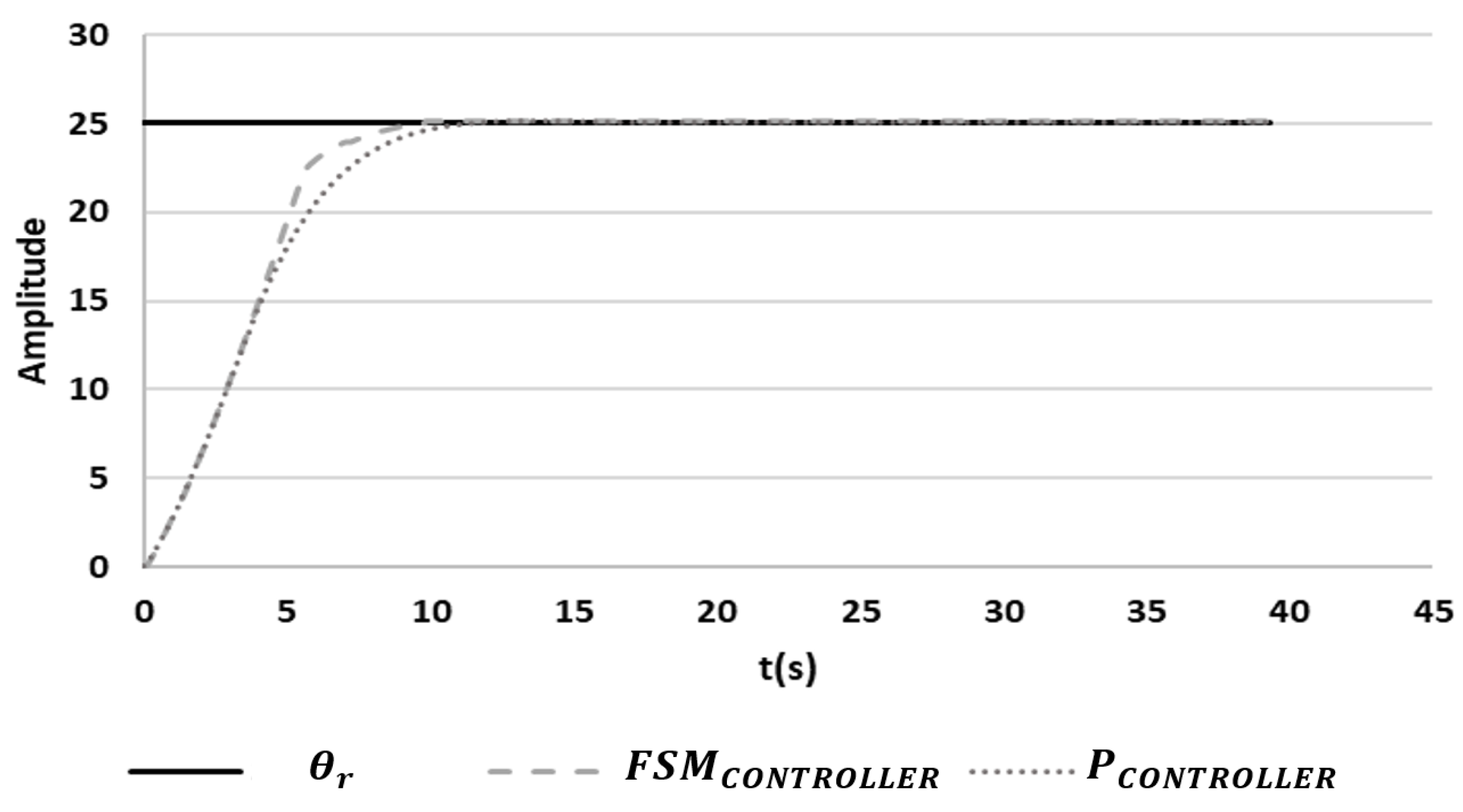
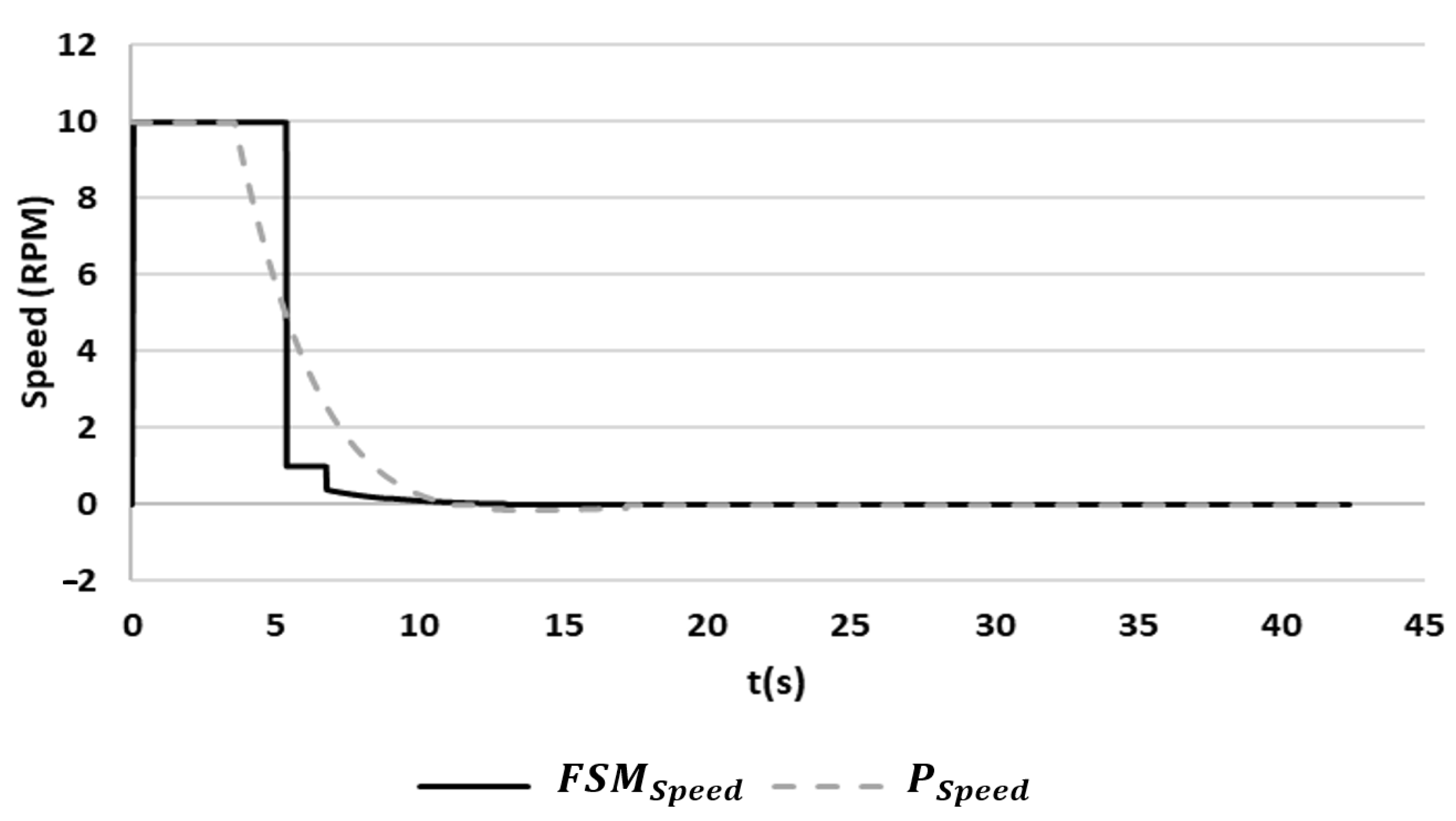
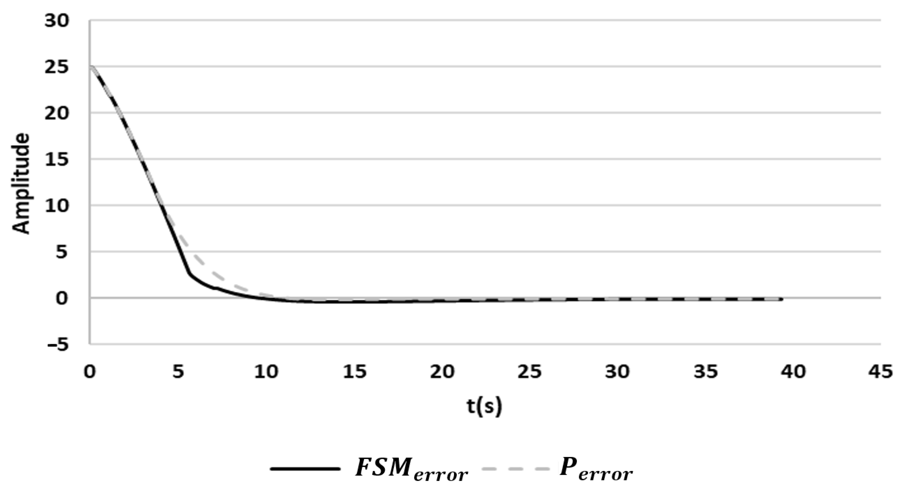
3.3.3. Comparison of FSM versus Proportional Controller

The proportional and FSM position controllers were evaluated using the IMC-PID speed controller. Maximum speed references were selected and applied to both controllers, and the closed-loop position control is compared below. In Figure 11, the response of the position variable is shown using the two control schemes. The response of the FSM controller was nonlinear; it approached the reference signal ${\theta }_r=25$ more quickly, and reached the desired value in 9.83 s. In comparison, the use of the position proportional controller settled the response in 11.33 s. The stability of the FSM controller is ensured by the controller transitions from one state to another.

The speed manipulations that the position controllers generate for the internal IMC-PID speed controller are compared in Figure 12. The speed set point that the proportional position controller generated was as expected, initially limited by the maximum speed and later computed to be directly proportional to the position error. The FSM controller generated two constant speed references: the maximum speed and then the constant deceleration speed. A zero-speed reference was finally reached at time $10.46 \mathrm{s}$ with the FSM, and at time 10.8 s with the P controller. The final approach occurred with a speed directly proportional to the small error, which could be incorporated with an additional approaching state within the FSM.

Figure 13 shows a comparison of the position errors generated while using the FSM and P position controllers. The error curves are similar except for the final transition phase. The FSM led to smaller errors as a function of an accelerated approximation to the set point value, with opportune deceleration to reach the final desired value with precision, i.e., without oscillation. The time integral of the absolute position error during the simulation test resulted to be 6% less for the case of the FSM controller with respect to the use of the P controller.

The following performance indices were considered: integral square error (ISE), integral absolute error (IAE), and integral of time multiplied absolute error (ITAE). These were evaluated for the FSM controller and the proportional controller cases during a simulation time of 20 s covering the transient response and assuring the final stabilization of the system. The performance indices are shown in

Table 2. Performance index of FSM control and proportional control.

Performance Index	FSM	$P$	%
ISE	74,466.68	78,257.19	4.84
IAE	4498.84	4814.55	6.56
ITAE	11,561.20	13,548.74	14.67

. The FSM position control had a better response than the only proportional controller according to the three indicators (ISE, IAE, and ITAE).

4. Results and Discussion

The virtual UR5 robot developed in Blender was implemented in a workstation with Modbus connectivity to an external SoftPLC running in the same workstation that can be remotely accessed. The virtual robot needs to be controlled in an HiL simulation scheme by means of programming the CoDeSys controller.

4.1. Results

The system was developed as an educational tool for online remote training on robotic arms particularly the UR type robot. The virtual robot is a visual interface with Modbus connectivity to an external controller, where the student faces the challenge to develop the code for modeling the actuators, designing and implementing the actuator control (angular speed and position), and programming the direct and inverse kinematic equations to be able to control the position and orientation of the robot.

Real-time control algorithms need to be developed by the user for the two critical levels of control of the robot: the independent joint position control and the inverse kinematic control for Cartesian position and orientation. The scheme of Figure 14 shows some possible control configurations that can be implemented. The first selector at the left is to enable the inverse kinematic control for the Cartesian positioning for the virtual robot for the direct operation of the joint angles. The second selector is to enable the position control with the herein proposed FSM-based position control that requires a servo-controlled dynamical response in the robot actuators.

Selectors switches can activate different settings for Cartesian mode, manual mode, normal mode, and test mode. Vector variables are used to refer to all the joint motors. $Q_R$ is the required value, $Q_{SP}$ is the reference value, $Q_M$ is the manual value, $Q_{VP}$ is the process variable value, and $Q_{COM}$ is the communication value. If the system is active in Cartesian mode, it performs inverse kinematics to calculate the required angular positions of all joints, copying the required positions to the position and velocity control reference values. If the system in Cartesian mode is not active, the manual mode is implied to give a direct reference to each joint; the manual values of each angle are copied to the reference values of the position and speed control. If the system is in test mode, it executes the control of all the joints, and then copies the value of the process variables to the communication variables. If the system in test mode is not activated, it does not execute the position control, and the values of the reference value are copied to the communication variables. The test mode is used to validate the inverse kinematics.

4.2. Discussion

In industrial robots applied in production lines, it is not necessary to know about actuator control or direct and inverse kinematic control; instead, it is required to learn the programming language to be able to program the automation tasks and interactions of the robot with the process. However, engineers working in robot design need to learn how to control the robot as a mechatronic system, i.e., considering the actuators and sensors, which implies the development of skills in control techniques at the actuator level, whereby the control of all the robot joints can be coupled with the kinematics control of the robot.

Robotic design courses which include kinematics and control are conventionally more theoretical since the robot controllers of commercial robots are considered as black boxes and normally can only be used for training robotics at the user level (task-oriented). The main feature of this implementation is to have separate entities: the virtual robot and the robot control system, as in real robotic systems that are made up of the physical robot and the control system. The developed systems help the students to learn practical concepts of robot kinematics and independent joint control that are two basic control levels that need to be implemented in the robotic arm design process. The developed system is a virtual UR5 robot that needs to be programmed for both the joint control level and the Cartesian control. Dynamical responses of the actuators and their position control can be modeled, programmed, simulated, and verified in the external controller. The inverse kinematic solution also needs to be programmed in the external controller for the control of the virtual robot to achieve a desired Cartesian position and orientation and eventually for trajectory tracking.

In this study, a novel joint position control strategy based on a finite state machine was implemented in a cascade configuration with a PID internal model control for speed control. The independent joint control strategy does not imply using the dynamic model of the robot, but only the dynamic model of the actuators, and they can be controlled for small variations in load torque as disturbances. The proposed control compensates for the dynamics of the motor; that is, if the joints are controlled, it can be said that the dynamics of the robot is controlled. This robust control allows monitoring the speed and has a torque estimator. This strategy for independent joint control was programmed and verified, and it was also combined with the inverse kinematic control to show the applicability of the developed system for the learning of robotic and control subjects.

5. Conclusions

Virtual laboratories have already been successfully implemented in universities and industries, for practical learning in postgraduate courses, workshops for students, or specialized training on automation, robotics, virtual automotive painting stations, and Industry 4.0 technology. The featured UR5 virtual robotic system was developed in Blender and requires an external controller with Modbus connectivity to control the 6DOF articulated virtual robot. To validate the developed system, inverse kinematics and motion control strategies are implemented in CoDeSys SoftPLC.

The UR5 virtual robot was developed following educational trends in technology based on the use of computer simulation and virtual reality applications. It uses the Radmin VPN software as remote control software, which allows us to connect to our virtual robot from anywhere and have full control over it. The main feature of this implementation is to have separate entities: the virtual robot and the robot control system, as in real robotic systems that are composed of the physical robot and the control system. The hardware in the loop architecture allows the development and verification of real-time control system of the UR5 robot, allowing users to test different control techniques through the ModBus communication protocol. In this study, a novel technique for the joint position control based on a FSM was proposed and verified with the virtual UR5 robots.

The proposed system was developed as an educational platform for the implementation of the required control algorithms, i.e., for the control of each of the robot’s joints and for the inverse kinematic control of the robot. Students can generate their own control algorithm and test it with the 3D robot simulator. In this way, users can develop and compare different control strategies in real time. Therefore, the system is a suitable platform to teach and learn the kinematics of the UR5 robot and its control. Further work will include the development of an application for task programing of virtual UR5 robot.

References

1. Olszewska, J.I. The Virtual Classroom: A New Cyber Physical System. In Proceedings of the 2021 IEEE 19th World Symposium on Applied Machine Intelligence and Informatics (SAMI), Herl’any, Slovakia, 21–23 January 2021; pp. 187–192. [Google Scholar] [CrossRef]
2. Pivoto, D.G.S.; de Almeida, L.F.F.; Da Rosa Righi, R.; Rodrigues, J.J.P.C.; Lugli, A.B.; Alberti, A.M. Cyber-physical systems architectures for industrial internet of things applications in Industry 4.0: A literature review. J. Manuf. Syst. 2021, 58, 176–192. [Google Scholar] [CrossRef]
3. Leng, J.; Zhang, H.; Yan, D.; Liu, Q.; Chen, X.; Zhang, D. Digital twin-driven manufacturing cyber-physical system for parallel controlling of smart workshop. J. Ambient. Intell. Humaniz. Comput. 2018, 10, 1155–1166. [Google Scholar] [CrossRef]
4. Pérez, L.; Rodríguez-Jiménez, S.; Rodríguez, N.; Usamentiaga, R.; García, D.F. Digital Twin and Virtual Reality Based Methodology for Multi-Robot Manufacturing Cell Commissioning. Appl. Sci. 2020, 10, 3633. [Google Scholar] [CrossRef]
5. Wuttke, H.D.; Henke, K.; Hutschenreuter, R. Digital twins in remote labs. In Cyber-Physical Systems and Digital Twins; Springer: New York, NY, USA, 2019; pp. 289–297. [Google Scholar] [CrossRef]
6. Verner, I.M.; Cuperman, D.; Gamer, S.; Polishuk, A. Training Robot Manipulation Skills through Practice with Digital Twin of Baxter. Int. J. Online Biomed. Eng. 2019, 15, 58–70. [Google Scholar] [CrossRef]
7. Rukangu, A.; Tuttle, A.; Johnsen, K. Virtual reality for remote controlled robotics in engineering education. In Proceedings of the IEEE Conference on Virtual Reality and 3D User Interfaces Abstracts and Workshops, VR Workshops 2021, Lisbon, Portugal, 27 March–1 April 2021; pp. 751–752. [Google Scholar]
8. Tselegkaridis, S.; Sapounidis, T. Simulators in educational robotics: A Review. Educ. Sci. 2021, 11, 11. [Google Scholar] [CrossRef]
9. Hao, C.; Zheng, A.; Wang, Y.; Jiang, B. Experiment Information System Based on an Online Virtual Laboratory. Future Internet 2021, 13, 27. [Google Scholar] [CrossRef]
10. Cobo, E.B.; Andaluz, V.H. Virtual Training System for Robotic Applications in Industrial Processes. In Augmented Reality, Virtual Reality, and Computer Graphics; AVR. Lecture Notes in Computer Science; Springer: Cham, Switzerland, 2021; Volume 12980, pp. 717–734. [Google Scholar] [CrossRef]
11. Cogurcu, Y.E.; Douthwaite, J.A.; Maddock, S. Augmented Reality for Safety Zones in Human Robot Collaboration. EG UK Comput. Graph. Vis. Comput. 2022, 1–7. [Google Scholar]
12. Alkhedher, M.; Mohamad, O.; Alavi, M. An interactive virtual laboratory for dynamics and control systems in an undergraduate mechanical engineering curriculum—A case study. Glob. J. Eng. Educ. 2021, 23, 55–61. [Google Scholar]
13. Arenas, F.; Martell, F.; Sanchez, I.Y.; Paredes, C.A. Virtual laboratory for online learning of UR5 robotic arm inverse kinematic and joint motion control. In Proceedings of the 2021 International Conference on Electrical, Computer and Energy Technologies (ICECET), Cape Town, South Africa, 9–10 December 2021. [Google Scholar]
14. Talli, A.; Meti, V.K. Design, simulation, and analysis of a 6-axis robot using robot visualization software. IOP Conf. Ser. Mater. Sci. Eng. 2020, 872, 12040. [Google Scholar] [CrossRef]
15. Wei, Z.; Li, Y. Design and simulation of robotic arm with light weight and heavy Load. In Proceedings of the 2nd World Conference on Mechanical Engineering and Intelligent Manufacturing: WCMEIM, Shanghai, China, 22–24 November 2019; pp. 537–540. [Google Scholar] [CrossRef]
16. Rout, J.; Agrawal, S.; Choudhury, B.B. Modeling and control of a six-wheeled mobile robot. Information and Communication Technology for Competitive Strategies. In Proceedings of the Third International Conference on ICTCS 2017, Udaipur, India, 16–17 December 2017; pp. 323–331. [Google Scholar] [CrossRef]
17. Villalobos, J.; Sanchez, I.Y.; Martell, F. Singularity Analysis and Complete Methods to Compute the Inverse Kinematics for a 6-DOF UR/TM-Type Robot. Robotics 2022, 11, 137. [Google Scholar] [CrossRef]
18. Jahnavi, K.; Sivraj, P. Teaching and learning robotic arm model. In Proceedings of the 2017 International Conference on Intelligent Computing, Instrumentation and Control Technologies (ICICICT 2017), Kerala, India, 6–7 July 2017; pp. 1570–1575. [Google Scholar] [CrossRef]
19. Villalobos, J.; Sanchez, I.Y.; Martell, F. Alternative Inverse Kinematic Solution of the UR5 Robotic Arm. In Advances in Automation and Robotics Research; LACAR 2021. Lecture Notes in Networks and Systems; Moreno, H.A., Carrera, I.G., Ramírez-Mendoza, R.A., Baca, J., Banfield, I.A., Eds.; Springer: Cham, Switzerland, 2022; Volume 347. [Google Scholar]
20. Sailan, K.; Kuhnert, K.D. DC motor angular position control using PID controller for the porpuse of controlling the hydraulic pump. In Proceedings of the International Conference on Control, Engineering & Information Technology, Sousse, Tunisia, 4–7 June 2013; pp. 22–26. [Google Scholar]
21. Arenas, F.; Martell, F.; Sanchez, I.Y. Discrete Time DC Motor Model For Load Torque Estimation For PID-IMC Speed Control. Mechatron. Syst. Control. 2022, 50, 102–108. [Google Scholar] [CrossRef]
22. Huang, G.; Lee, S. Pc-based PID speed control in DC motor. International conference on audio, language and image processing. In Proceedings of the International Conference on Audio, Language and Image Processing, Shanghai, China, 7–9 July 2008; pp. 400–407. [Google Scholar]
23. Ihechiluru, S.; Enwerem, C.O. Performance assessment of a model-based dc motor scheme. Appl. Model. Simul. 2019, 3, 145–153. [Google Scholar]
24. Ahmed, U.O.; Patrick, A.A.; Kwembe, B.A. DC Motor Speed Control using Internal Model Controller Industrial Transformation Strategy. Int. J. Eng. Adv. Technol. 2020, 9, 300–306. [Google Scholar] [CrossRef]
25. Al Tahtawi, A.R.; Somantri, Y.; Haritman, E. Design and Implementation of PID Control-based FSM Algorithm on Line Following Robot. JTERA (J. Teknol. Rekayasa) 2016, 1, 23–30. [Google Scholar] [CrossRef]
Figure 1. Virtual robot proposed configuration.
Robotics 12 00023 g001
Figure 2. The 3D model of Robot UR5.
Robotics 12 00023 g002
Figure 3. UR5 robot base frame.
Robotics 12 00023 g003
Figure 4. Block diagram of the DC motor model.
Robotics 12 00023 g004
Figure 5. IMC-PID speed control.
Robotics 12 00023 g005
Figure 6. Cascade position (P) and speed (PID) control scheme.
Robotics 12 00023 g006
Figure 7. Proportional position control.
Robotics 12 00023 g007
Figure 8. Cascade position (FSM) and speed (PID) control.
Robotics 12 00023 g008
Figure 9. State diagram of the position controller. The position error is represented by e 1 . S and D denote stop and deceleration error values, subscripts n and p indicate negative and positive values, and ω is the required angular velocity which can be minimum (MIN) or maximum (MAX). Adapted with permission from ref. [13]. Copyright 2021 IEEE.
Robotics 12 00023 g009
Figure 10. Position control using FSM-IMC-PID.
Robotics 12 00023 g010
Figure 11. Position controller comparison: FSM and proportional.
Robotics 12 00023 g011
Figure 12. Comparison of manipulations.
Robotics 12 00023 g012
Figure 13. Error comparison of FSM-IMC-PID versus P-IMC-PID.
Robotics 12 00023 g013
Figure 14. Configuration scheme of Cartesian mode and test mode.
Robotics 12 00023 g014