

Based on the Foot–Ground Contact Mechanics Model and Velocity Planning Buffer Control
1
Department of Mechanical and Electrical Engineering, Northeast Forestry University, Harbin 150040, China
2
Locomotive and Car Research Institute, China Academy of Railway Sciences, Beijing 100081, China
*
Author to whom correspondence should be addressed.
Robotics 2023, 12(1), 17; https://doi.org/10.3390/robotics12010017
Submission received: 20 December 2022
/
Revised: 16 January 2023
/
Accepted: 20 January 2023
/
Published: 23 January 2023
(This article belongs to the Special Issue The State-of-the-Art of Robotics in Asia)
Abstract
:In order to reduce the impact of the leg joint motors and body electric devices of a falling robot, active flexible control based on force and velocity is proposed. A velocity planning buffer method based on a virtual model is proposed. We established a mechanical model of leg and ground contact. Then, we controlled the knee joint angular velocity change after the robot contacted the ground to reduce the collision impact force and to protect the robot’s joint motors and body’s internal parts. First, the relationship between contact force and velocity was analyzed through the contact mechanical model between leg and ground, and the target was determined. Then, by planning the velocity of the robot’s thigh and hip joint, the velocity mutation during contact was reduced so that the impact on the robot was reduced. This method can avoid complex accurate physics model building and complex torque signal interference filtering processing, the control process is simple and its effectiveness is verified by ADAMS simulation and experimental verification. The velocity planning buffer strategy was tested in experimental studies which showed that the contact force of the buffer strategy was 0.671 times that of no buffer. Additionally, the contact impact acceleration of velocity planning was 1.5505 g, which was less than the force 1.7 g of virtual model control. The velocity planning buffer strategy was better to protect the robot.
1. Introduction
Forest terrain is complex; various shapes of obstacles can be seen everywhere [1], and mobile forest robots may fall from the obstacles. When a robot makes contact with the ground it will produce impact, which will damage the overall structure of the robot and the body’s internal parts [2]. We should control contact impact as far as possible. In the research in related fields, scholars made the actual leg or arm structures equivalent to virtual “spring-damping” systems and control the contact force by adjusting the stiffness and damping coefficient [3]. The other method is by adding a Serial Elastic Actuator [4,5] to improve the flexibility of the robots. Zhang Haibo et al. [6], through the LaGrange’s equations of second kind, established a general kinematic model of the spatial robot and a dynamic model of the point-surface collision in contact with the environment to design the force/pose hybrid control and the force/torque ring control. The force/pose hybrid controller is obtained by complying with the selection matrix. Additionally, through the error between the actual contact force and the expected contact force, it obtains the force control and matrix of the joint torque value, which reduces the impact collision of the end of the robot. However, the LaGrange dynamics model of this method is complex, and the control law requires high model precision. Sun Xinchao et al. [7] put forward an adaptive variable impedance control method that can adjust the internal impedance control parameters in real time. This method avoids the large force tracking error and the unstable control system caused by the constant traditional impedance control parameters. Additionally, this method achieves the accurate force tracking control. However, the impedance adaptive controller needs to adjust the stiffness and damping of the system during a short interaction process, and the control process is complex. Dong Yunfei et al. [8] proposed that contact force is detected and controlled through the motor encoder and joint torque sensor. Additionally, through a robot dynamic model and efficient adaptive filter, strong vibration and surface radian interference are effectively avoided in the contact process. Liu Bin et al. [9,10] reduced the impact on the leg–ground by setting the acceleration of the body and the expected trajectory of the foot during the collision process. The process of control is adding a virtual “spring-damping” system between the foot’s actual and desired position. Liu Chunjian et al. [11] have designed a hydraulic servo, passive flexible joint, which has good flexibility and can adjust the position feedback when a collision occurs. Shao Nianfeng et al. [12] used a series elastic drive (SEA) to improve the robot’s joint flexibility and achieve a certain buffer effect. Luo Jianxiong et al. [13] based the hydraulic rotation corner servo on the compliant joint. The active compliant control, in the event of a collision, reduced the over concussion, which was obtained by the variable stiffness method of the cam four-link mechanism. Wang Xinping et al. [14] have designed a new variable stiffness flexible joint to improve the safety of human–computer interaction during the collision. Feng Zhiyou et al. [15] have designed a new type of variable-damping flexible drive joint that is controlled by a parallel adhesive damping adjustable module. Navid Dini et al. offered using a nonlinear disturbance observer as a virtual force sensor, which can reduce permanent errors in the case of fast varying external forces. The tracking control optimizes the accelerations of the leg joints of the robot [16]. Zhu An et al. used the Lagrange function based on dissipation theory and the Newton–Euler function, respectively, to establish the dynamics model of the robot. Then, they combined Newton’s third law and the law of conservation of energy to establish the closed-chain dynamics. Then, they calculated the impact effects and impact force using the closed-chain dynamics. Based on the barrier Lyapunov function, they designed the control method [17]. Gong Chi-yu et al. offered a compliant control strategy in which the outer loop adopts a global fast terminal sliding mode controller. Additionally, the inner loop uses a force-based PD control to make the contact force, track the expected force and reduce the impact [18]. In previous studies, the robot was well-buffered in contact with the environment, together with adaptive impedance control and stiffness control. However, the process of impedance control is complex in adjusting stiffness, damping parameters are complicated and a large number of tests are needed in the process of adjusting parameters. In this paper, we propose a velocity buffer method, which, by establishing the mechanical model of leg–ground contact, an active flexible control method based on impulsive dynamics is proposed.
The rest of this paper is organized as follows. Section 2 describes the foot–ground model and the velocity planning, explains the theory of the velocity planning buffer strategy and introduces the theory model. Section 3 describes the simulation and the experiment of the velocity planning, simulating and testing to verify the velocity planning buffer strategy. Section 4 summarizes the main results of this research.
2. Contact Mechanics Model and Velocity Planning
When analyzing the contact impact force, firstly, the mechanical model of the contact between the leg and ground was established. Additionally, the structure diagram of the robot leg’s forward direction is shown in Figure 1. The leg structure of the robot can be seen as a rigid body. The leg’s forward direction has two coaxial rotating joints, respectively, the forward direction hip joint and the knee joint. The joint angle of the forward direction hip joint is q1, and the joint angle of the knee joint is q2. The other parameters of the model are shown in Table 1.
The coordinate system{x1ox2} is the body coordinate system; the x1 axis is in the horizontal direction, and the positive direction is in the reverse direction of travel. The axis x2 is in the vertical direction, and the positive direction is under the vertical phase. Under the coordinate system{x1ox2}, the end of the leg (x1(t),x2(t))can be expressed by Equation (1):
where q(t)1 is the variable quantity of the angle of the hip joint and q(t)2 is the variable quantity of the angle of the knee joint. q(t)1 and q(t)2 are expressed by Equation (2):
Fr is the force received in the axial direction of the leg, Fr′ is the separation force of the contact surface method of phase direction and Fr″ is the separation force of the tangential direction. Fr′ and Fr″ are defined by Equation (3):
Using statics and the principle of virtual work, we established the equation of contact forces and the joint torques shown by Equation (4):
where τ1 is torques of the normal force, τ2 is torques of the tangential force and JT is the Jacobian matrix, which is defined by Equation (5):
When two rigid bodies make contact with a certain velocity, a constraint arises in the contact surface that prevents the two rigid bodies from embedding within each other [19]. Under the law of conservation of energy and the contact constraints, the rigid body velocity changes, and the impulsive force is generated between the two rigid bodies.
The separation force of the contact surface method of phase direction Fr′ can be defined by Equation (6):
where Fc is the reaction force of the contact impact force in normal direction and Fi is the force of support phase ground to the leg.
The reaction force of the contact impact force established by the impulsive dynamics is expressed by Equation (7):
where f(t) is the force generated on the foot contact surface in Δt time and t0 is the initial time of contact.
The effect of the impulsive force is to change the momentum of the leg system. Additionally, the equation of motion of the leg system’s momentum and force during the robot contact is defined by Equation (8):
where I is the inertia of the leg in movement space and relates to the mass, a(t) is the acceleration of the leg in Δt time and v(t) is the velocity of the leg in Δt time.
Most of the mass of the leg is the joint, hip and thigh. So, we made the hip and the thigh fixed, and the inertia means the hip and the thigh connector are calculated and deduced according Equation (9):
Then, the reaction force of the contact impact force in normal direction Fc can be defined by Equation (10):
It is known that the reaction force of contact impact force Fc is proportional to the change of the body and thigh’s velocity Δv in Δt time. So, to reduce the contact impact force, the change of linear velocity Δv in time Δt can be planned to be as small as possible.
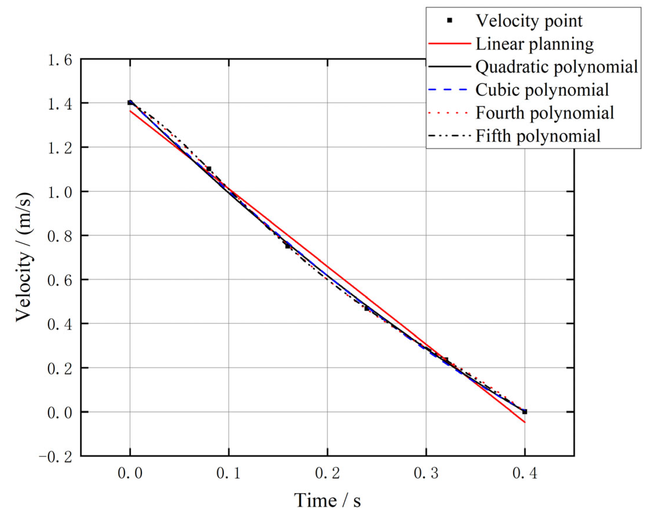
Then, establishing the velocity planning, the mutations of velocity need to be controlled to be as small as possible. Now, the falling height of the robot was set as 100 mm, and the velocity of the robot was 1.4 m/s when the foot made contact with the ground. Velocity planning was planned using the constrained polynomial curve with boundary conditions. The common polynomial curves are primary linear planning, quadratic polynomial, cubic polynomial, fourth polynomial and fifth polynomial. Once the limited values were inputted, we calculated the polynomial linear planning curve through MATLAB. The result is shown in Figure 2.
It can be seen from the curves in Figure 2 that the primary linear curve cannot meet the requirements of the initial and final values. The quadratic polynomial meets four velocity points. The cubic polynomial, fourth polynomial and fifth polynomial are relatively close and can meet all velocity points. In order to simplify the planning process, we selected cubic polynomial for planning. Additionally, the cubic polynomial is defined by Equation (11):
To set the boundary constraints: (1) in the foot–ground contact, the acceleration change is zero, so that the contact velocity is the maximum value in the time interval; (2) the change of acceleration is monotonically small; (3) the constraint acceleration final value is . Through the initial value and boundary constraints, the velocity polynomial is defined by Equation (12):
Additionally, the joint angular velocity is expressed by Equation (13):
3. Simulation and Experimental Results
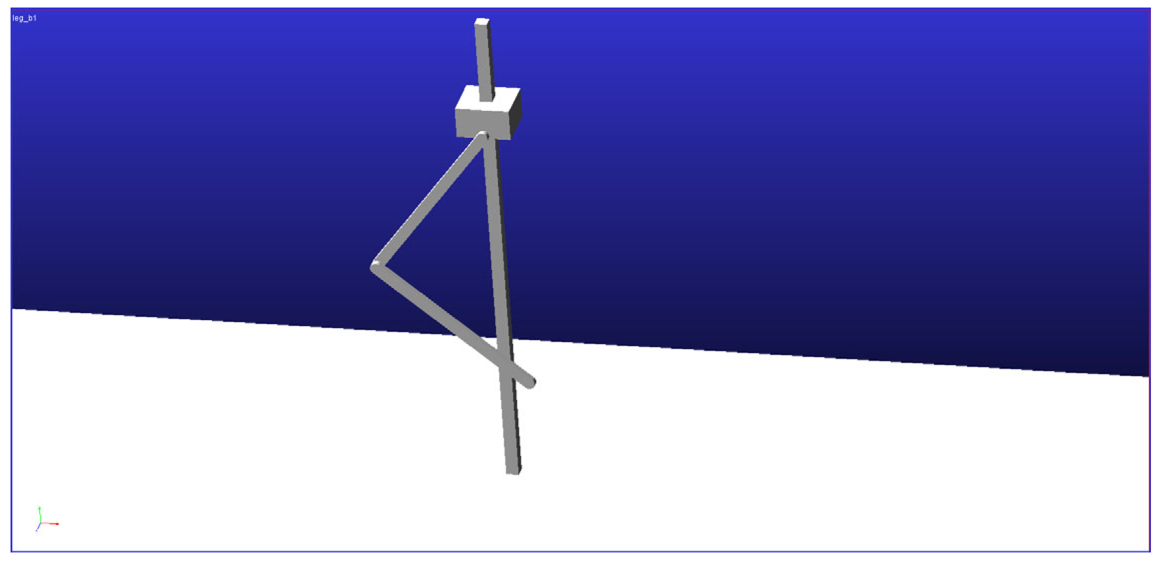
For testing the effectiveness of the velocity planning buffer strategy, we built a testing model using 3D modeling software and then input the model into ADAMS to simulate it. The simulation model is shown in Figure 3.
The qualities of the hip, thigh and shank in ADAMS were inputted by users. Then, we set the center of mass position and inertia as the default values. We set the rotation of the hip joint to 0 * time, and set the center of mass position of the body and thigh connecting. The quality of each part of the robot is shown in Table 2.
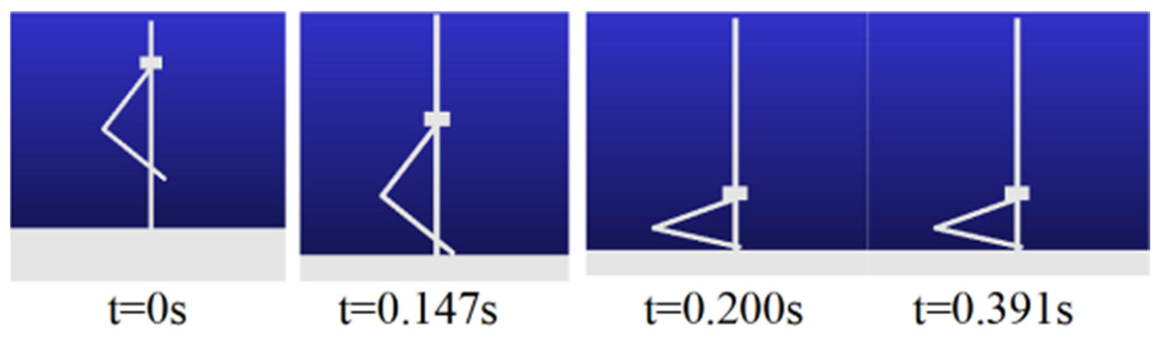
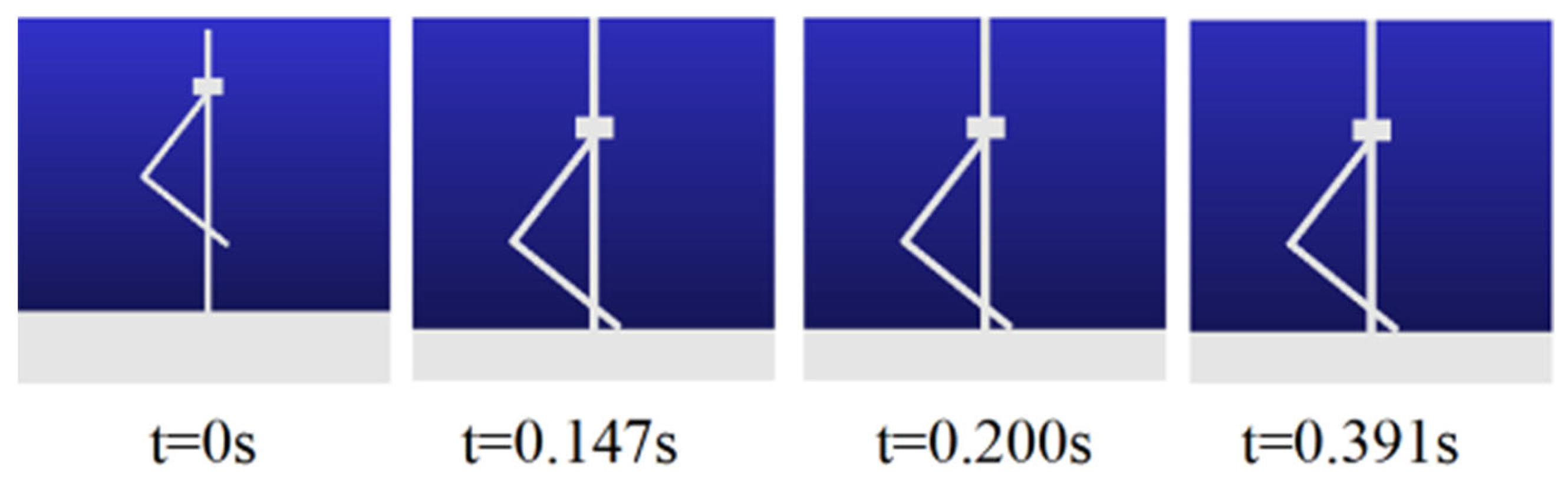
The revolute pairs were added to the positions of hip with thigh and thigh with shank. Additionally, the revolute pairs’ friction coefficients were set as the default value. The initial falling height was 100 mm, and the gravity acceleration as the default direction was the negative direction of the global coordinate system Y. The screenshot of the simulation test process is shown in Figure 4 and Figure 5; Figure 4 is a screenshot of the simulation test with buffer process, and Figure 5 is a screenshot of the simulation test without buffer process. At t = 0 s, the robot is at 100 mm from the ground; at t = 0.147 s, the robot foot contacts the ground and at t = 0.391 s, the robot buffer process ends.
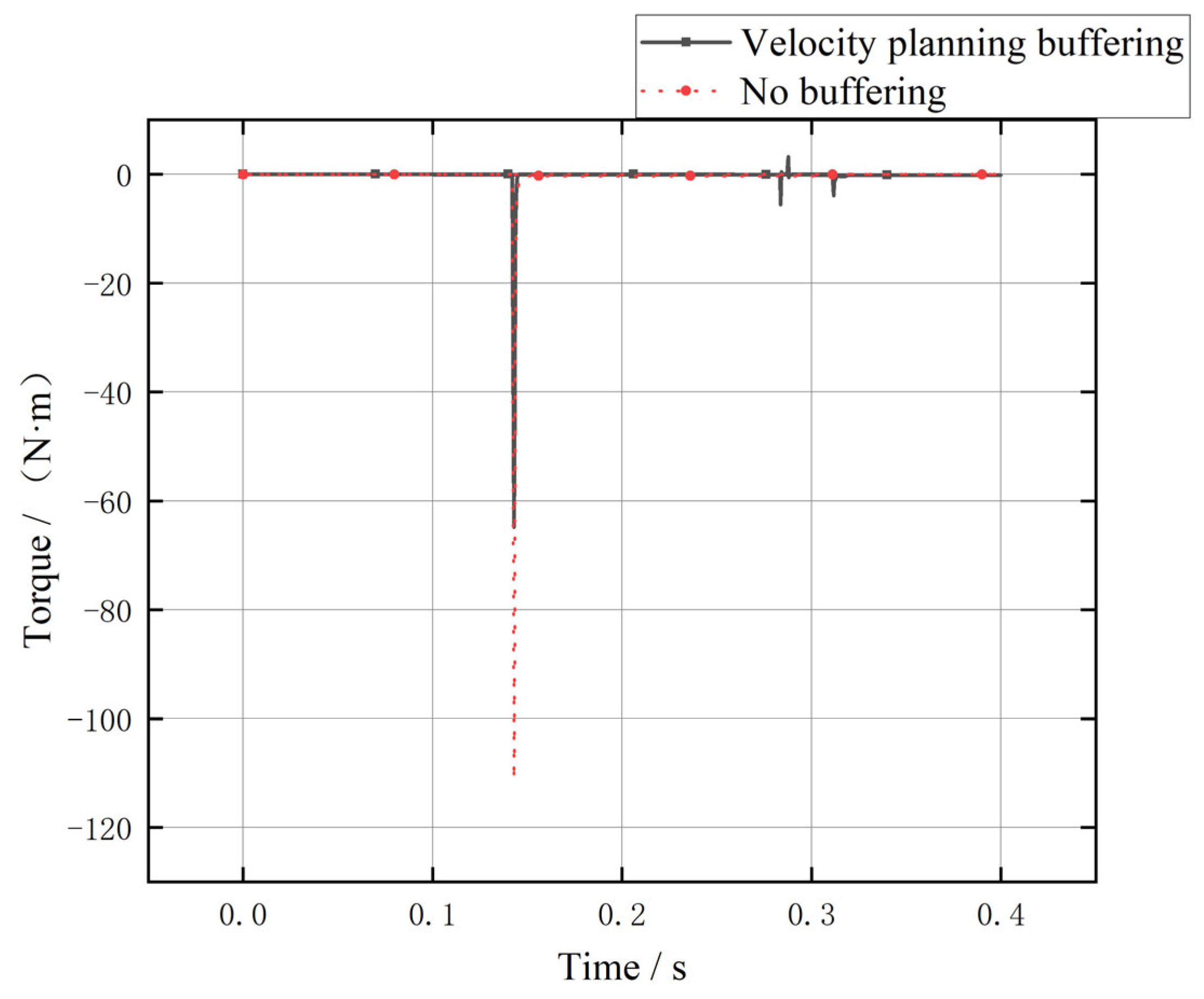
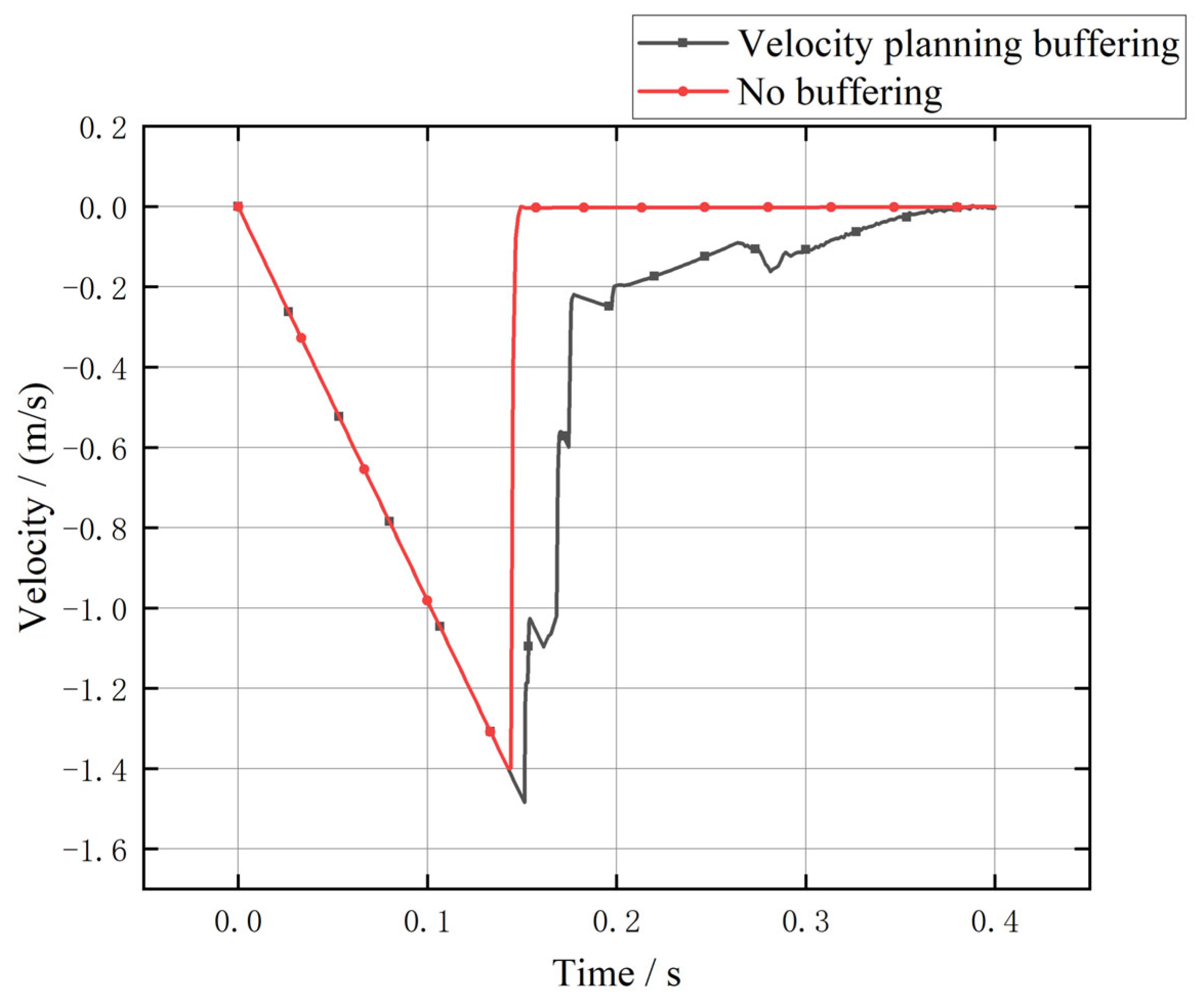
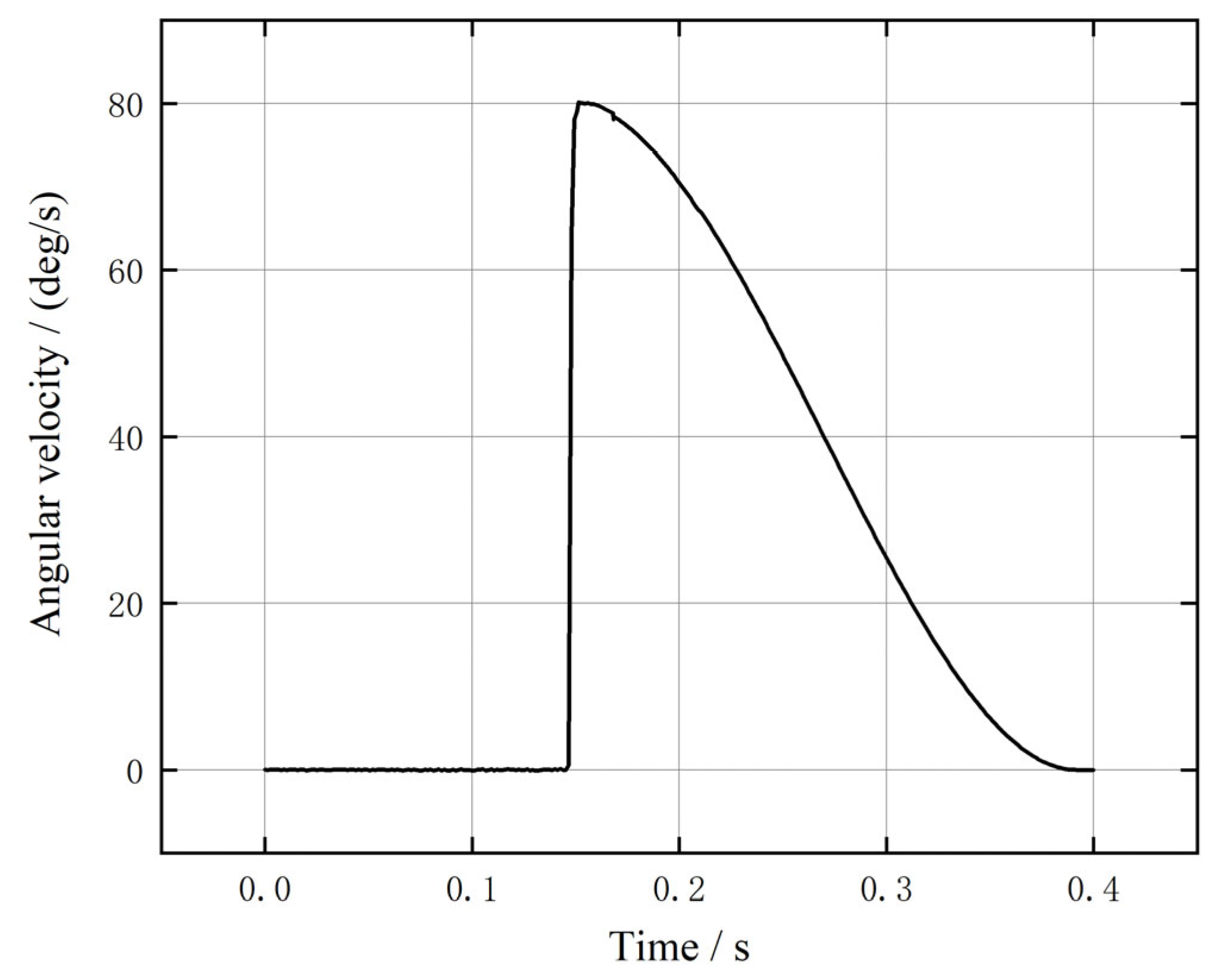
Then, we measured the torques of the knee joints, the velocity of COM and the knee joint angular velocity change with velocity planning buffering. The results are in Figure 6, Figure 7 and Figure 8.
We can find the joint torque in Figure 6, and we can see that the peak of velocity planning buffering is lower than with no buffering. So, we deemed that the peak torque had been optimized and the velocity buffering was effective. The peak of velocity planning was 0.5830 times of the peak with no buffer. The velocity and angular velocity of the knee joint was used to guide the experiment.
Then, we prepared the experiment to test the theory, model and simulation. Due to the torque transducer being too large and not easy to fix, we chose the one-dimensional pressure pickup to measure the contact force.
The process of the velocity planning buffer was to reduce the contact speed mutation of the thigh and hip joint, which reduced the contact force and contact impact. The realization process was to change the rotation velocity of the knee joint during contact, obtain the rotation velocity of the knee joint through ADAMS simulation and then the motor was controlled in the experiment.
In the experiment, we preset the rotation velocity of the motor, whose value is the knee angular velocity obtained by the ADAMS simulation, and then set the S-shaped curve deceleration using the Sigmoid function. When the foot force sensor detected the force data, the motor rotated at a predetermined velocity.
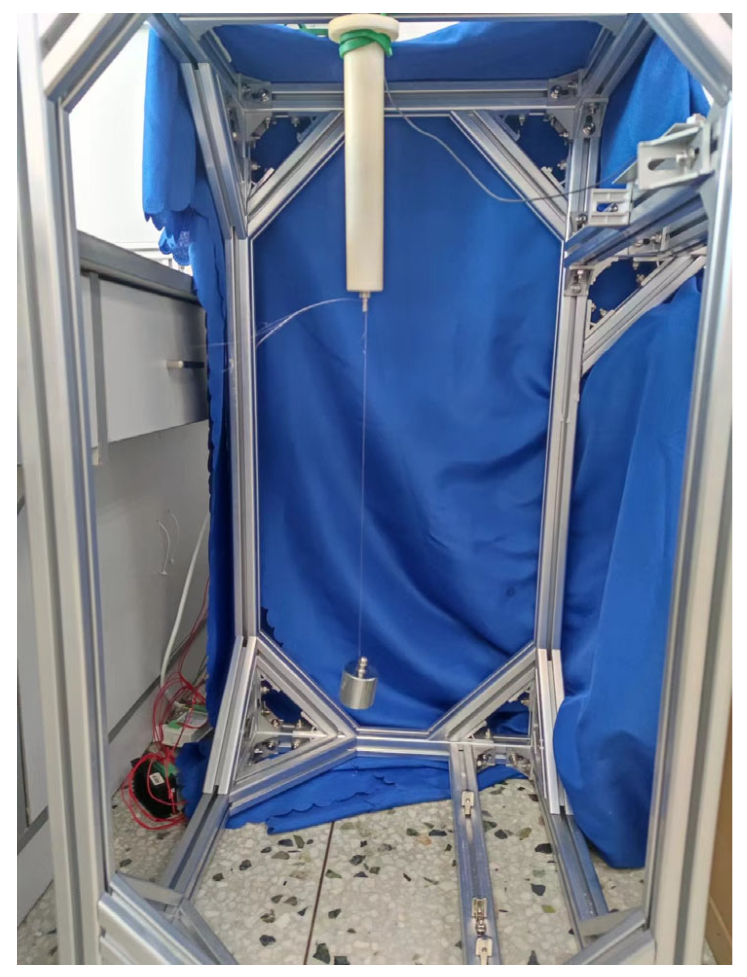
After software debugging, structural assembly and wiring, we calibrated the one-dimensional pressure pickup. We fixed the shank, which was loaded with pressure pickup, on the aluminum profile and trussed up the weights beneath the pressure pickup as shown in Figure 9.
The steps for calibration were:
- (1)
- Hold up the bottom of the weight by hand and release the weight after the voltage value is stable to make it droop naturally. Observe the oscilloscope at the upper machine end and record the voltage value and the weight mass through the upper machine storage module.
- (2)
- Repeat the operation in (1), measure one set of mass weights several times and replace the mass combination of other weights. The above steps are repeated to obtain the multiple sets of voltage and weight mass data of the seven weight mass combinations.
After the calibration experiment, we obtained the relationships of voltage and weight quality shown in Table 3.
Through searching, it was known that the gravity acceleration in Harbin is 9.806 m/s2, so, using the least square method, we fit the relationship as defined by Equation (14):
where v is voltage.
Fr = 67.3999 v + 4.0161
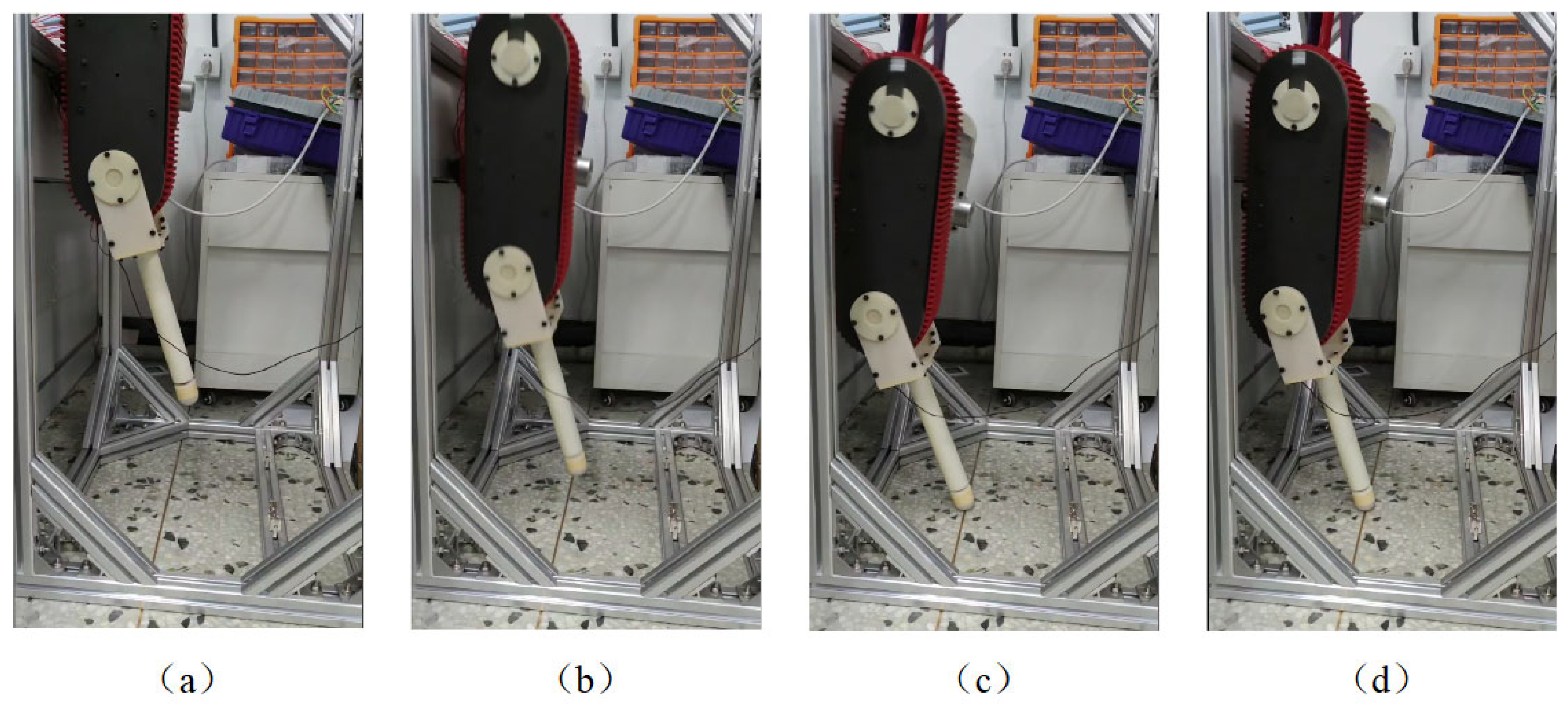
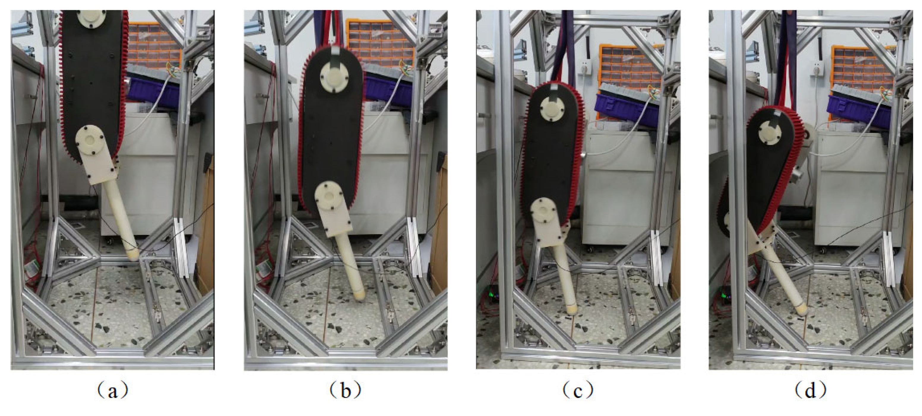
The final experiment tested the velocity planning buffer. The process of the experiment was to relax the elastic rope to make the one leg fall freely; the elastic rope could only maintain the balance within the single-leg roll plane. The experiment was divided into one with buffer experiment and the control group without buffer experiment, as shown in Figure 10 and Figure 11. First, we lifted the single leg up to the preset height (which was same as the simulation model height, 100 mm) by lifting ropes. Then, we unlashed the lifting ropes and the single leg began to free-fall. We tested twice. In the first test the single leg contacted the ground with no buffer. Additionally, in the second test the single leg contacted the ground with the velocity planning buffer strategy. The process of no-buffer contact is shown in Figure 10 and Figure 10a is the single leg in lifting. Figure 10b is the state of free-fall, Figure 10c is the moment the single leg contacted the ground and Figure 10d is keeping contact and the leg with no buffer. The process of the velocity planning buffer contact is in Figure 11; Figure 11a,b is same as Figure 10a,b, Figure 11a shows the leg lifting and Figure 11b shows the leg in free-fall state. Figure 11c is the moment the single leg made contact with the ground and the knee joint began to revolve (the angular velocity set as simulation results). Figure 11d shows the single leg finish the velocity buffer strategy.
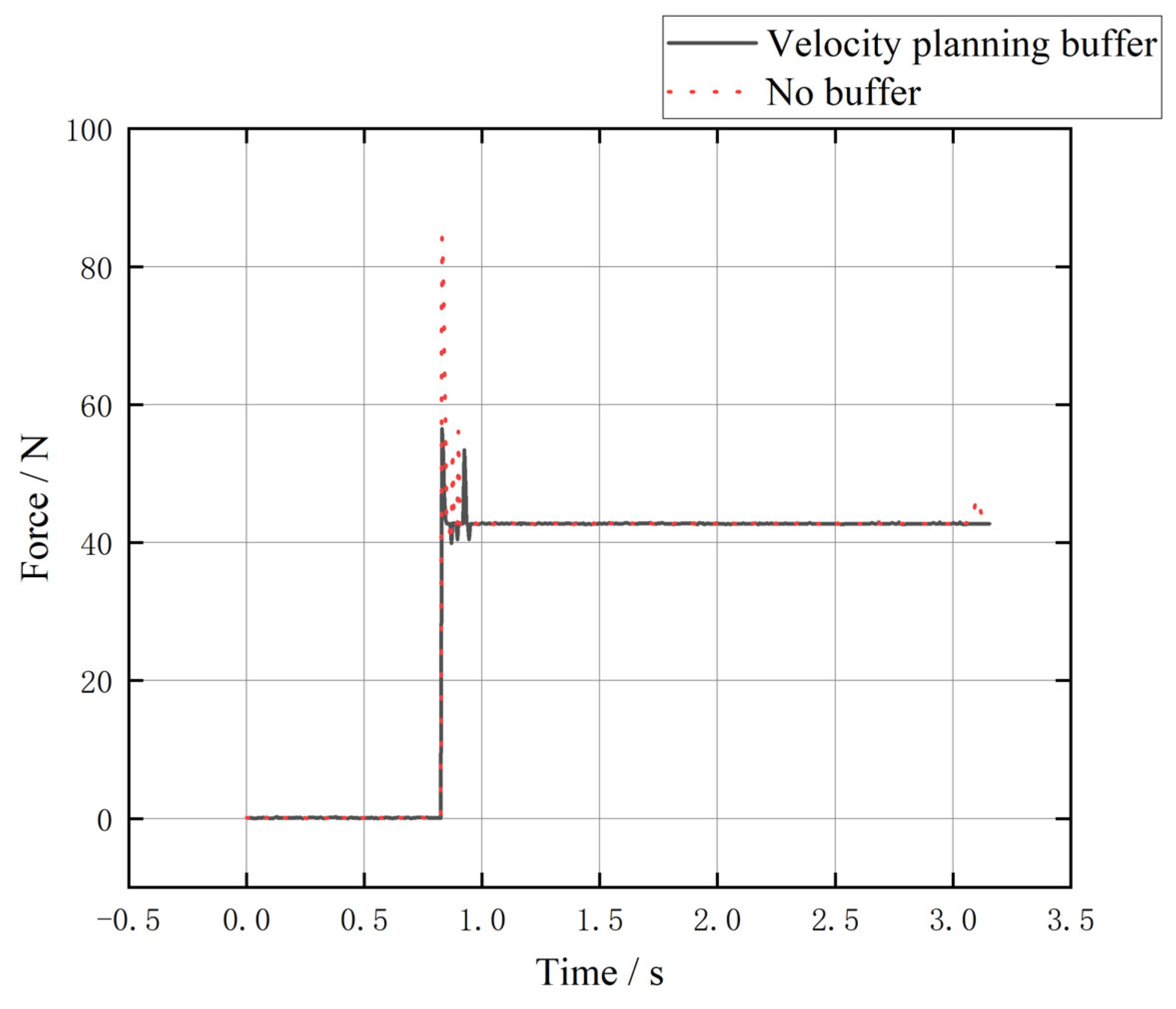
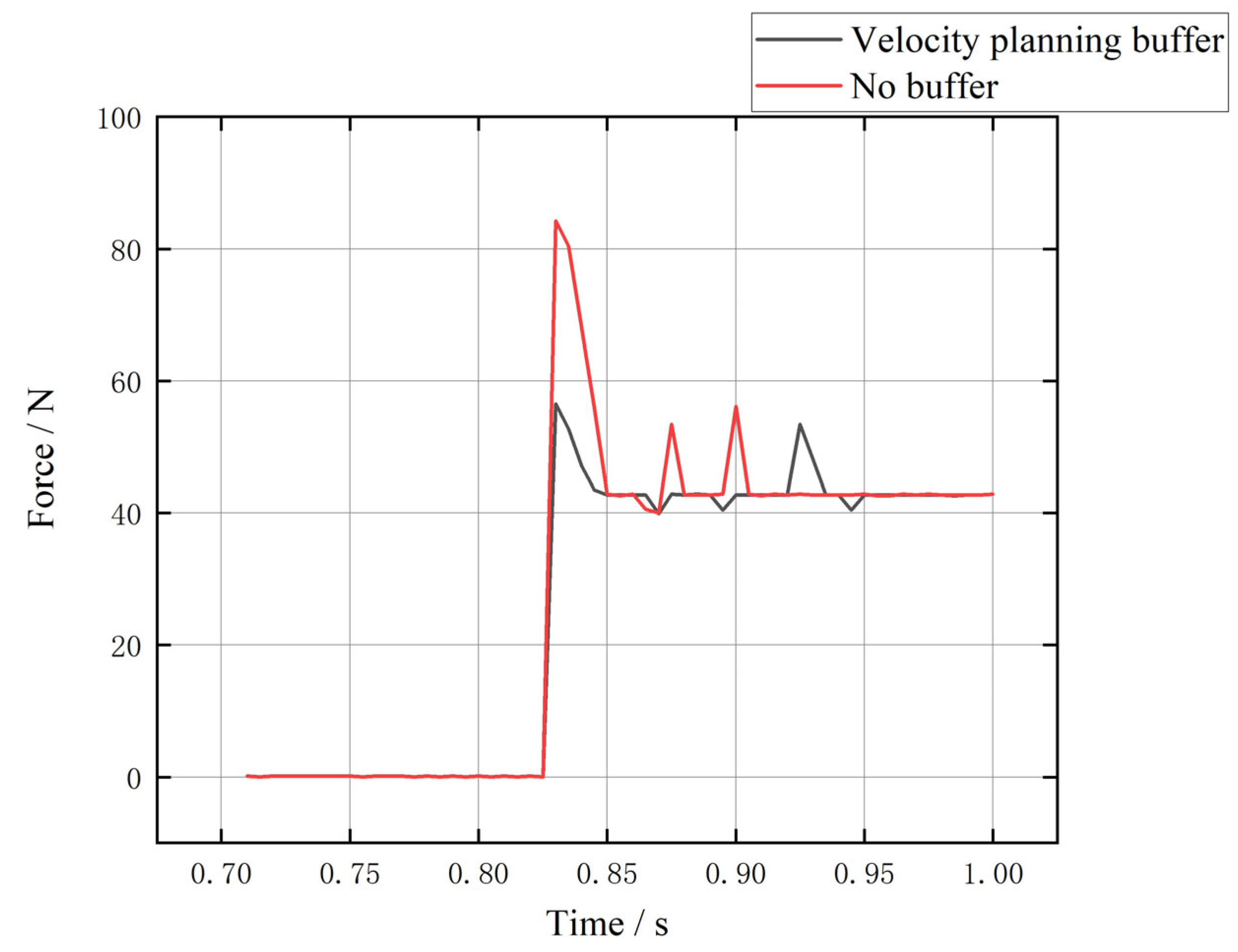
The data of the foot end pressure pickup in the experiment are shown in Figure 12, 0 s to 0.825 s, showing the leg in the lifting and free-fall. The contact happened at 0.825 s, and from 0.825 s to 1.0 s the leg was in the course of buffering. From 1.0 s to 3.2 s the leg continued contact with ground. The meaningful part of the experiment was included in the 0.7 s to 1.0 s, so we show the part’s data in Figure 13. The single-leg experimental bench produced a large instantaneous impact force with no buffer contact moment, the same as expected from the pulse dynamics of the simulation. After introducing the buffer strategy based on speed planning, the contact instantaneous impact had obvious optimization. The velocity planning contact force was 0.671 times that of no-buffer, because the simulation model parameters set in motion vice static friction. The friction coefficient setting had certain differences with the actual experimental bench, so the results are not exactly the same, but the force change trend was similar. The test results show that they are confirmed our expected outcome from the simulation.
By calculating the data of contact force, we found that the peak of contact force of the velocity planning buffer strategy was 1.5505 g (g, which is the leg mass), while the buffer strategy controlled by the virtual model mentioned in [20], which had a peak contact force of about 1.7 g. Compared with the buffer strategy controlled by the virtual model, the velocity planning buffer strategy reduced the impact acceleration and the velocity planning buffer strategy had better protection effects for the robot.
4. Conclusions
In this paper, we proposed a novel buffer strategy for a leg robot where the mass of thigh and hip was heavier than that of the shank. It was based on a leg–ground contact mechanical model and rigid bodies impulsive dynamics. By using impulsive dynamics analysis to obtain the velocity planning buffer strategy, it availably reduced the contact force; the contact force was only 0.671 times that of no buffer contact. All of the above makes the buffer strategy a perfect fit for robots with a mass of the thigh and hip heavier than that of the shank.
Author Contributions
Conceptualization, B.Z., L.W. and Y.W.; methodology, B.Z.; software, B.Z.; validation, B.Z., Y.W., L.W. and Z.Y.; formal analysis, B.Z.; investigation, B.Z.; resources, Y.W.; data curation, B.Z.; writing—original draft preparation, B.Z. and L.W.; writing—review and editing, B.Z., L.W. and Y.W.; visualization, B.Z.; supervision, Y.W.; project administration, Y.W.; funding acquisition, Y.W. All authors have read and agreed to the published version of the manuscript.
Funding
This research received no external funding.
Data Availability Statement
Not applicable.
Conflicts of Interest
The authors declare no conflict of interest. The funders had no role in the design of the study; in the collection, analyses, or interpretation of data; in the writing of the manuscript; or in the decision to publish the results.
References
- Jiang, P.F.; Liu, Y.H.; Zhou, J.B.; Fu, W.S.; Zhang, B.; Chang, F.H. Development and research status of forestry field robots. For. Grassl. Mach. 2020, 1, 20–27. [Google Scholar] [CrossRef]
- Lou, W.T. Mathematical Modeling and Collusion Analysis of Foot and Ground Interaction of Hydraulic Drive Robot; Yanshan University: Qinhuangdao, China, 2021. [Google Scholar] [CrossRef]
- Sun, T.; Cheng, L.; Peng, L.; Hou, Z.; Pan, Y. Learning impedance control of robots with enhanced transient and steady-state control performances. Sci. China Inf. Sci. 2020, 63, 192205. [Google Scholar] [CrossRef]
- Zhang, Q.C. Development of Lower Limb Exoskeleton Based on Series Elastic Actuator; Yanshan University: Qinhuangdao, China, 2021. [Google Scholar] [CrossRef]
- Zhong, H.R. Bipedal Robot Motion Control Based on Hydraulic Series Elastic Actuator; Huazhong University of Science and Technology: Wuhan, China, 2021. [Google Scholar] [CrossRef]
- Zhang, H.B.; Wang, D.T.; Wei, C.L. Contact Dynamics Model of Refueling Device and Compliance Control for Space Robots. Chin. Space Sci. Technol. 2015, 35, 1–9. [Google Scholar]
- Sun, X.; Zhao, L.; Liu, Z. A model reference adaptive variable impedance control method for robot. MATEC Web Conf. 2021, 336, 03005. [Google Scholar] [CrossRef]
- Dong, Y.; Ren, T.; Hu, K.; Wu, D.; Chen, K. Contact force detection and control for robotic polishing based on joint torque sensors. Int. J. Adv. Manuf. Technol. 2020, 107, 2745–2756. [Google Scholar] [CrossRef]
- Liu, B.; Chai, W.X.; Chai, H. A Buffering Strategy for Quadrupedal Robots Based on Virtual Model Control. Robot 2016, 38, 659–669. [Google Scholar] [CrossRef]
- Liu, B.; Song, R.; Chai, H. Buffering Strategy for Articulated Legged Robot Based on Virtual Model Control and Acceleration Planning. J. Shandong Univ. Eng. Sci. 2016, 46, 69–75. [Google Scholar]
- Liu, J.C.; Jiang, L.; Ren, L.S.; Zhou, L.; Zhao, H. Compliance Characteristics of A Hydraulic Servo Passive Compliant Joint. J. Wuhan Univ. Sci. Technol. 2021, 44, 270–276. [Google Scholar]
- Shao, N.F.; Zhou, Q.Y.; Shao, C.; Zhao, Y. Research on Joint Compliance of Robot Based on SEA. Modul. Mach. Tool Autom. Manuf. Tech. 2020, 11, 33–37+41. [Google Scholar] [CrossRef]
- Luo, J.X.; Zhao, H.; Jiang, L. Active Compliance Control Based on Hydraulic Manipulator. J. Wuhan Univ. Sci. Technol. 2022, 45, 127–134. [Google Scholar]
- Wang, X.Q.; Liu, Y.L.; Li, S.Q.; Shao, C.Y.; Zhao, C. Design and Analysis of A New Type of Variable Stiffness Compliant Joint. Chin. J. Constr. Mach. 2021, 19, 506–511. [Google Scholar] [CrossRef]
- Feng, Z.Y.; Xu, W.B.; Zhi, D.; Kang, R.J.; Chen, L.S. Design of Robot Compliant Driving Joint with Variable Damping. J. Tiangong Univ. 2019, 38, 76–81. [Google Scholar]
- Dini, N.; Majd, V.J. Sliding-Mode Tracking Control of a Walking Quadruped Robot with a Push Recovery Algorithm Using a Nonlinear Disturbance Observer as a Virtual Force Sensor. Iran. J. Sci. Technol. Trans. Electr. Eng. 2020, 44, 1033–1057. [Google Scholar] [CrossRef]
- Zhu, A.; Ai, H.P.; Chen, L. Compliance Control of Dual-arm Space Robot Capture Satellite Based on Barrier Lyapunov Functions. China Mech. Eng. 2022, 33, 2997–3006. [Google Scholar] [CrossRef]
- Gong, C.K.; Xu, A.D.; Yuan, L.P. Compound Anti-interference Compliant Control for Quadruped Robot Under Unknown Rugged Terrain. Control Engineering of China. 2022. Available online: https://read.cnki.net/web/Journal/Article/JZDF20220722000.html (accessed on 19 January 2023).
- Mirtich, B. Impulse-Based Dynamic Simulation of Rigid Body Systems; University of California at Berkeley: Berkeley, CA, USA, 1996. [Google Scholar]
- Liu, B.; Zhang, M. A hybrid control strategy for legged robot buffering in landing process. J. Shandong Univ. Eng. Sci. 2022, 52, 20–28+37. [Google Scholar]
Figure 1.
Leg–ground contact mechanical model.

Figure 2.
Polynomial linear planning curves.

Figure 3.
The simulation model.

Figure 4.
The screenshot of the buffer simulation process.

Figure 5.
The screenshot of the no-buffer simulation process.

Figure 6.
The torque of the knee joint.

Figure 7.
The velocity of the COM of hip and thigh.

Figure 8.
The curve of angular velocity change of knee joint.

Figure 9.
The calibration of pressure pickup.

Figure 10.
(a–d) Single leg with no buffer contact.

Figure 11.
(a–d) Single leg with velocity planning buffer contact.

Figure 12.
The data of the foot end pressure pickup in the experiment.

Figure 13.
The part data from 0.8 s to 1.0 s in the experiment.


Table 1.
Model; the parameters of the leg–ground model.
| Parameter Symbol | Parameter Name | Parameter Value |
|---|---|---|
| Thigh Length | 300 mm | |
| Shank Length | 300 mm | |
| Velocity of body COM | - | |
| Falling Height | - | |
| Force in shank direction | - |
Table 2.
The parameters of model quality.
| Parts | Quality/kg |
|---|---|
| hip | 8 |
| thigh | 8 |
| shank | 3 |
Table 3.
The weight masses corresponded to the voltage value.
| Weight Quality/kg | Voltage/V |
|---|---|
| 0.5 | 0.0654609 |
| 1 | 0.0824768 |
| 1.5 | 0.1079786 |
| 2 | 0.2222822 |
| 2.5 | 0.3110214 |
| 3 | 0.3725367 |
| 3.5 | 0.458001 |
Disclaimer/Publisher’s Note: The statements, opinions and data contained in all publications are solely those of the individual author(s) and contributor(s) and not of MDPI and/or the editor(s). MDPI and/or the editor(s) disclaim responsibility for any injury to people or property resulting from any ideas, methods, instructions or products referred to in the content. |
© 2023 by the authors. Licensee MDPI, Basel, Switzerland. This article is an open access article distributed under the terms and conditions of the Creative Commons Attribution (CC BY) license (https://creativecommons.org/licenses/by/4.0/).
Share and Cite
MDPI and ACS Style
Zhang, B.; Wang, L.; Wang, Y.; Yuan, Z. Based on the Foot–Ground Contact Mechanics Model and Velocity Planning Buffer Control. Robotics 2023, 12, 17. https://doi.org/10.3390/robotics12010017
AMA Style
Zhang B, Wang L, Wang Y, Yuan Z. Based on the Foot–Ground Contact Mechanics Model and Velocity Planning Buffer Control. Robotics. 2023; 12(1):17. https://doi.org/10.3390/robotics12010017
Chicago/Turabian StyleZhang, Boxuan, Lichao Wang, Yangwei Wang, and Zehao Yuan. 2023. "Based on the Foot–Ground Contact Mechanics Model and Velocity Planning Buffer Control" Robotics 12, no. 1: 17. https://doi.org/10.3390/robotics12010017
Note that from the first issue of 2016, this journal uses article numbers instead of page numbers. See further details here.