Optimal Design of Energy Sources for a Photovoltaic/Fuel Cell Extended-Range Agricultural Mobile Robot

Abstract

Powertrain electrification in the agricultural vehicles is still in the initial stages. This article analyzes the energy behavior of a Photovoltaic/Fuel Cell Agricultural Mobile Robot (PV/FCAMR) as the preliminary step before development. This concept incorporates three energy storage sources for the powertrain: a battery pack, a Fuel Cell (FC) system, and a Photovoltaic (PV) system. This paper proposes an approach based on the Grey Wolf Optimization (GWO) and Particle Swarm Optimization (PSO) algorithms to determine the sizes of the FC and battery of an FCAMR. A differential drive mobile robot was used as a case study to extract the typical working cycles of farming applications. The FCAMR vehicle model was developed in MATLAB/Simulink to evaluate vehicle energy consumption and performance. For the energy analysis and evaluation, the FCAMR was tested based on two realistic working cycles comprising circular and rectangular moving patterns. The results showed that the proposed arrangement could extend the FCAMR autonomy by 350% as opposed to the pure electric system. This allows for at least 8 h of work with a tank filled with 150 g hydrogen and a PV system with a 0.5 m${}^2$ monocrystalline solar panel. The simulation results have demonstrated the relevance and robustness of this approach in relation to various working cycles. The cost comparison between the theoretical and optimization sizing methods showed at least an 8% decrease for the FCAMR. Furthermore, adding the PV system extended the vehicle’s range by up to 5%. This study provides an optimal solution for energy sources sizing of mobile robots as futuristic agricultural vehicles.

1. Introduction

Today, the world’s population is increasingly growing and is currently reaching around eight billion [1]. At the same time, the demand for food and agricultural products continues to increase as living standards improve. Meanwhile, the increase in the urban population and the decrease in the rural population have also promoted the development and application of new agricultural machinery due to the labor shortage issues. On the other hand, the agriculture sector faces several challenges, such as increasing energy demand, greenhouse gas emissions, and the effects of global warming [2]. Therefore, the farm machinery of the future must be completely redesigned. It should be modular with exchangeable equipment integrated into the machine, autonomous, and lightweight. Thus, several small vehicles can operate in the field simultaneously, working continuously, 24 h a day, automatically changing equipment and batteries/refueling when needed [3].

The development of agricultural robot technology is an inevitable requirement for agriculture to find solutions to the challenges related to the shortage of labor, precision control, farm work convenience, and green operation. Such challenges are difficult to solve with conventional agricultural machinery, which has an important carbon footprint [4]. As a result of the research efforts, there are several robotic solutions addressing several different areas such as monitoring [5], mapping [6], crop and pest managing [7], environmental control [8], phenotyping [9], and planting [10]. For example, the researcher in [11] developed an original LiDAR-based high-throughput phenotyping system for cotton plant phenotyping in the field. The Hortibot [12] is a robotic tool carrier for high-tech plant care. In addition, the ByeLab [13] mobile vehicle has been developed to monitor and sense the health status of orchards and vineyards. In another application, Vibro Crop Robotti [14] can also perform field work such as mechanical weeding and precision seeding. Recently, an Ackermann steering control system was developed and tested successfully for a four-wheel-drive agricultural mobile robot in [15]. Moreover, in [9,16] the navigation problems of mapping, localization, and path planning in navigation problems of agriculture wheeled mobile robots were reviewed and the application prospects were discussed. They mentioned that, due to the agricultural environment’s complexity, the available methods still need to be improved in their practicability and effectiveness. In this regard, the research in [17] used a Robotic Operating System (ROS)-based simulation method to overcome the phenotyping bottleneck in the real farm situations. Recently, advances in agriculture robotics and challenges ahead were reviewed in the comprehensive survey in [18].

We have mentioned only some examples, but many more projects on mobile agriculture platforms have been started worldwide. However, most of them have been unsuccessful in their mission due to battery limitations and energy shortages. Moreover, regarding the electric powertrain design aspect, a solar-powered unmanned ground vehicle was studied in [19] for precision agriculture. However, the technical details of the sizing and selection of the components have not been made available in the literature.

The main drawback of conventional agricultural machines is the high consumption of fossil fuels, which has resulted in large emissions of harmful gases. The depletion of fossil fuels and their adverse environmental impact have motivated governments and communities to look for strategies enabling pollution-free renewable energy sources for vehicle applications [20]. Therefore, tractors with internal combustion engines are neither safe nor healthy, especially in closed working environments such as greenhouses. Based on information from the Environmental Protection Agency (EPA), around 38 percent of greenhouse gas emissions are from the transportation, agriculture, and industry sectors [21]. In this regard, the use of clean technologies such as powertrain electrification and alternative energy has been proposed as a solution [22]. The literature shows that some progress has been made in the case of agricultural tractors [23,24]. Still, hybridized powertrains for agricultural robots have not received enough attention. Therefore, using new agricultural machinery such as robotic systems and electrified vehicles is essential to achieve lower emissions, higher fuel efficiency, and increased controllability [25]. On the other hand, the use of robotics in agriculture has contributed to solving some problems. For instance, in closed or semi-closed environments, such as greenhouse and warehouse applications, there are two major issues. First, the fossil fuel combustion in engines releases air pollution, which is harmful to the workers. Second, the working environment could be affected by high engine noise levels. This is why most agricultural robots are powered by an electric propulsion system, bringing many advantages such as improved efficiency, and powertrain design flexibility [26].

A battery storage system is still one of the most limiting technologies for many electric mobile platforms such as robots [27]. Some non-road vehicles, such as forklifts and warehouse robots, already have a long history of using electric propulsion systems [28]. However, the low durability and long recharging time of the current batteries have created limitations in electric vehicles’ autonomy and performance, such as for AMRs in farm applications. These limitations would be more drastic when the vehicles are working in harsh environments such as large farms and greenhouses, which can increase the user cost under multi-shift working conditions during the working season. In addition, the electric AMRs must be charged after a certain operating period. However, in a real situation, a vehicle with nearly empty batteries is unavailable in the working process. Moreover, the failure of a vehicle on a farm while performing a task can result in a catastrophe, and it might cause many problems for farmers. Furthermore, using an electric vehicle with a low battery State of Charge (SOC) might reduce the battery’s lifetime [29,30].

In recent years, FCs have gained popularity due to their high-power generation efficiency, non-polluting, fast fueling, acceptable energy density, and low noise. In an FC range extended (FCREx) architecture, the secondary power source (FC) produces electricity to supply power as battery assistance. An FCREx mainly relies on batteries for power and is equipped with an FC system to extend the range of a basic battery-powered system. Regarding various kinds of FC technologies, proton exchange membrane fuel cells (PEMFCs) have higher operating efficiencies up to 70% compared to ICEs with less than 30% [31]. In addition, the PEMFC has a less cyclic operation, resulting in longer lifetimes and less system control design issues [32]. In this respect, hybridizing the vehicle’s power supply using the battery and a PEMFC system as a range extender could reduce the size of the FC stack, slowing power transients. Meanwhile, peak power is drawn into the battery system. This could reduce cost and volume in the vehicle design process.

This research focuses on developing optimal solutions for the design of a renewable energy-based (fuel cells + PV) hybrid configuration for an electric mobile robot in agricultural application. The main idea is to design a Fuel Cell Agricultural Mobile Robot (FCAMR) with the basic capabilities of a robotic system with low emission, no charge anxiety, and safe operation. The goal is to extend the autonomy so the vehicle can be operated for an entire day without needing to recharge the electrical system. Compared with the traditional agricultural vehicles, which closely follow the manufacturing process of automobiles, the agricultural robot industry is more complex, and there are not enough standards for these machines. As an outline, the current study discusses the design concerns of a renewable energy-based hybrid electric agricultural mobile robotic concept which is discussed rarely in literature. An FCAMR model developed in MATLAB/Simulink and two Optimization algorithms from Particle Swarm optimization (PSO) and Grey Wolf optimization (GWO) are proposed to simulate and optimize the vehicle. The rest of this paper is organized as follows: The project background, designing process, and modeling for an AMR as a case with an experimental tests procedure are given in Section 2. Section 3 describes a sizing design process based on the optimization algorithms and model in the loop process. Results are presented and discussed in Section 4. Finally, conclusions are drawn in Section 5.

2. Materials and Methods

2.1. Project Background

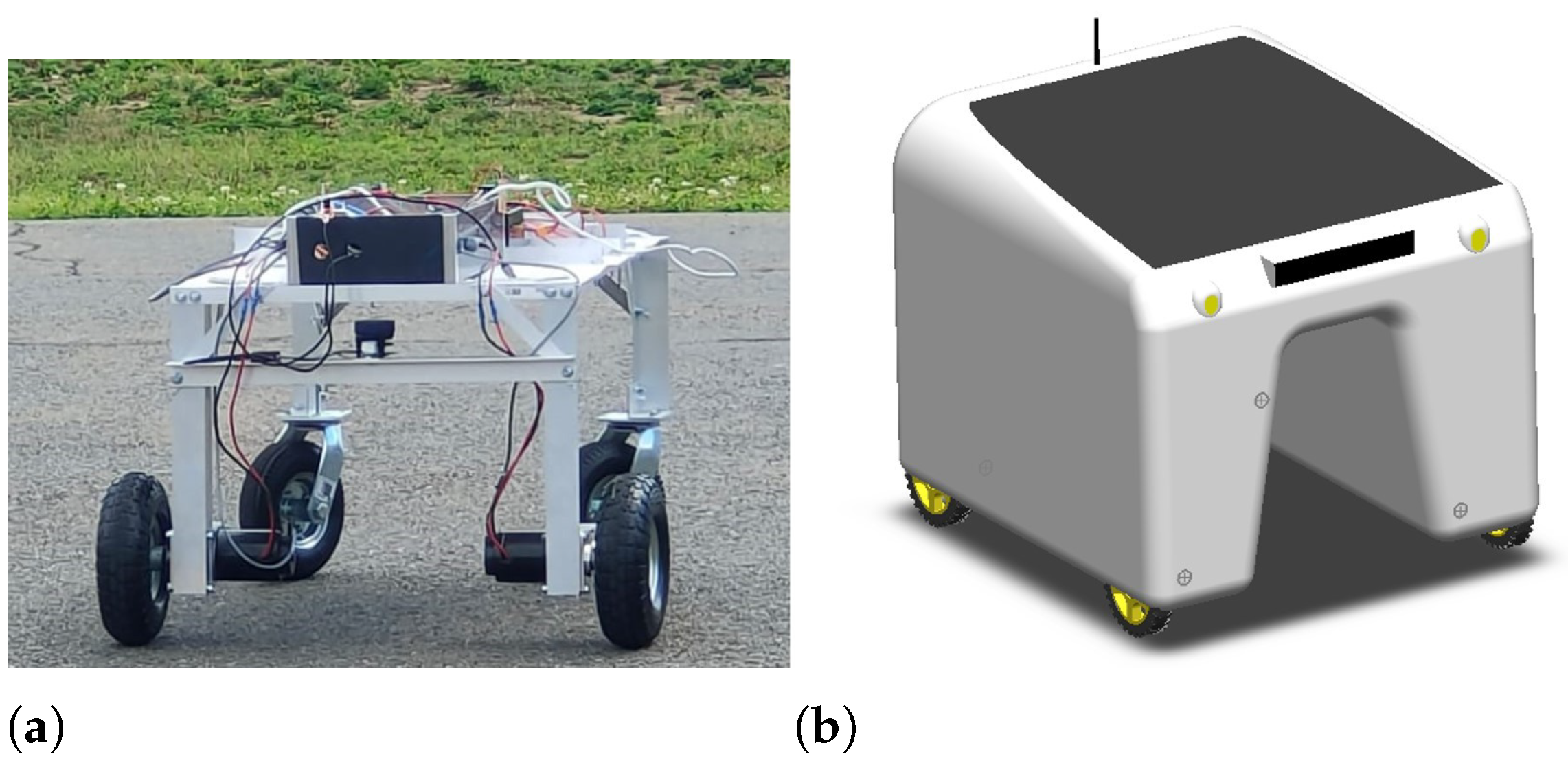
In this research, a battery-powered agricultural robot which was designed by our research team at University of Quebec in Trois-Rivieres and considered as a case study for developing a PV/FC/battery hybrid electric mobile robot for agricultural applications. This robot contains two main criteria, including software structure and hardware structure. The software structure contains control strategies, designing and developing path plan algorithms, energy management systems, etc. On the other, the hardware structure contains aspects such as component sizes, and electronic and electrical circuits, which are described in the following sections. The hardware structure of the case study AMR was made by considering the design requirements. Therefore, the differential drive–steering method was used to navigate the robot. Figure 1 presents the studied AMR. The robot powertrain consists of two electric motors with single-speed gearboxes (16:1 aspect ratio) for each driven wheel. In this context, the regenerative braking system is neglected due to the low-speed application and drive control limitation.

The AMR stored position data in a time series database using sensors such as an Inertial Measurement Unit (IMU), Global Positioning System (GPS), encoders, and Light Detection and Ranging (LIDAR). In addition, an onboard computer (Raspberry Pi) was utilized to compute localization, navigation algorithms, and data acquisition. A remote control system is equipped to manually control the robot at a visual distance. The data acquisition system monitors the wheels’ speed and the battery status by measuring the battery voltage and current drawn from the battery pack.

Table 1. The main electrical and electronic components specifications of the AMR [33].

Element	Description
LIDAR Sensor	YDLIDAR X2
GPS	BN-220
IMU	MPU-6050
Wheel Encoders	US Digital E3-500-375-NE-E-D-3
Main Microprocessor	ARM Cortex-A72 processor
Main Microcontroller	Atmega 328p
Current Sensor	LEM CAS 25-NP
Motor Controller	AF160
Motors	Ampflow E30-150-12-G16

shows the specifications of the AMR’s main electrical and electronic components. The AMR can be operated in manual (remotely controlled) and autonomous modes. A remote-control system is equipped to manually control the robot at a visual distance which is used for primary working cycle measurement in the predefined paths. Moreover, the AMR relies on a Lidar-based algorithm for obstacle detection and to avoid collision with workers and crops [33].

The primary energy system was designed according to the requirements of the drive system including a 24 Ah lead acid battery pack. The analysis is specially set during June 2022, when the working cycle can begin at 8 a.m. and end at 18 p.m., which would require making at least 8 h of work.

Based on the experimental tests, the vehicle could not make more than three hours at an average speed of $1.2$ m/s under typical working conditions. Choosing a bigger battery would not be reasonable due to the cost, weight, and environmental concerns. Therefore, it decided to hybridize the powertrain system by using more environmentally friendly power sources.

2.2. Proposed Design Process for the PV/FCAMR Architecture

Despite acceptable energy efficiency in basic pure electric AMR, because of the inherent limitations of the battery-powered vehicles, it was faced with a lack of energy in long-time operations due to the limited capacity and fast degradation of the battery. One of the opportunities for solving the problem of autonomy is to incorporate a PV system to collect free energy from the sun while doing farm tasks outside during the day. In addition, using PV panels could protect the AMR because most of the farm tasks are outside under the possibility of harsh environments such as rain, sun, and dust. Moreover, these could increase the energy independence of the robot on faraway farms. Another option is to integrate a modular PEMFC system with a hydrogen tank as an energy source that can be refuelled in less than five minutes [22] as opposed to a battery with several hours of recharging time. Regarding the architecture of the designed AMR, the FCREx powertrain configuration seems to be more applicable in an FCAMR application because of its flexibility and simplicity. Similar to the series hybrid electric architecture, the FCREx is a battery dominant system which uses a FC as an alternative for the internal combustion engine. Indeed, this architecture allows a secondary power source (FC) to operate at its optimal region, belong its more flexible location option for the designer [34]. For previous reasons, a plug-in PV/FC hybrid-electric configuration is considered a suitable powertrain for the AMR application because it can connect to the electric grid and might be charged from external electric power sources such as stationary solar power plants as well. This system has three energy sources: a battery pack, an onboard PV system, and a hydrogen tank with FC. A simplified powertrain for the proposed plug-in hybrid PV/FC-AMR is presented in Figure 2.

In fact, the design and development of non-road agricultural hybrid electric vehicles is a complex process; nevertheless, there is no standard methodology. Therefore, a general design process of the hybrid PV/FCAMR is proposed in this paper. In this regard, the following steps are considered. First, define typical farm working cycles based on customer needs. Next, modeling an AMR for component sizing and EMS evaluation before construction. Then, designing and developing a PV/FC range extender system. After that, designing and developing a heuristic EMS. Finally, components integration and evaluation of the hybrid electric FCAMR. In the following sections, the design process is discussed in detail.

2.3. Working Cycle Design and Extraction

Concerning performance assessment, conventional vehicles are usually tested in specific conditions using different dynamometers. Several standard driving cycles are used in the automotive development [34]. For non-road vehicles, if standardized tests exist, they are still unrepresentative of all real-world applications, since every application is inherently different. Based on the author’s knowledge, there is no standard working cycle for agricultural robots. Therefore, one of the main challenges of the AMR simulation is the lack of standardized drive cycles, which makes comparing results from different studies difficult.

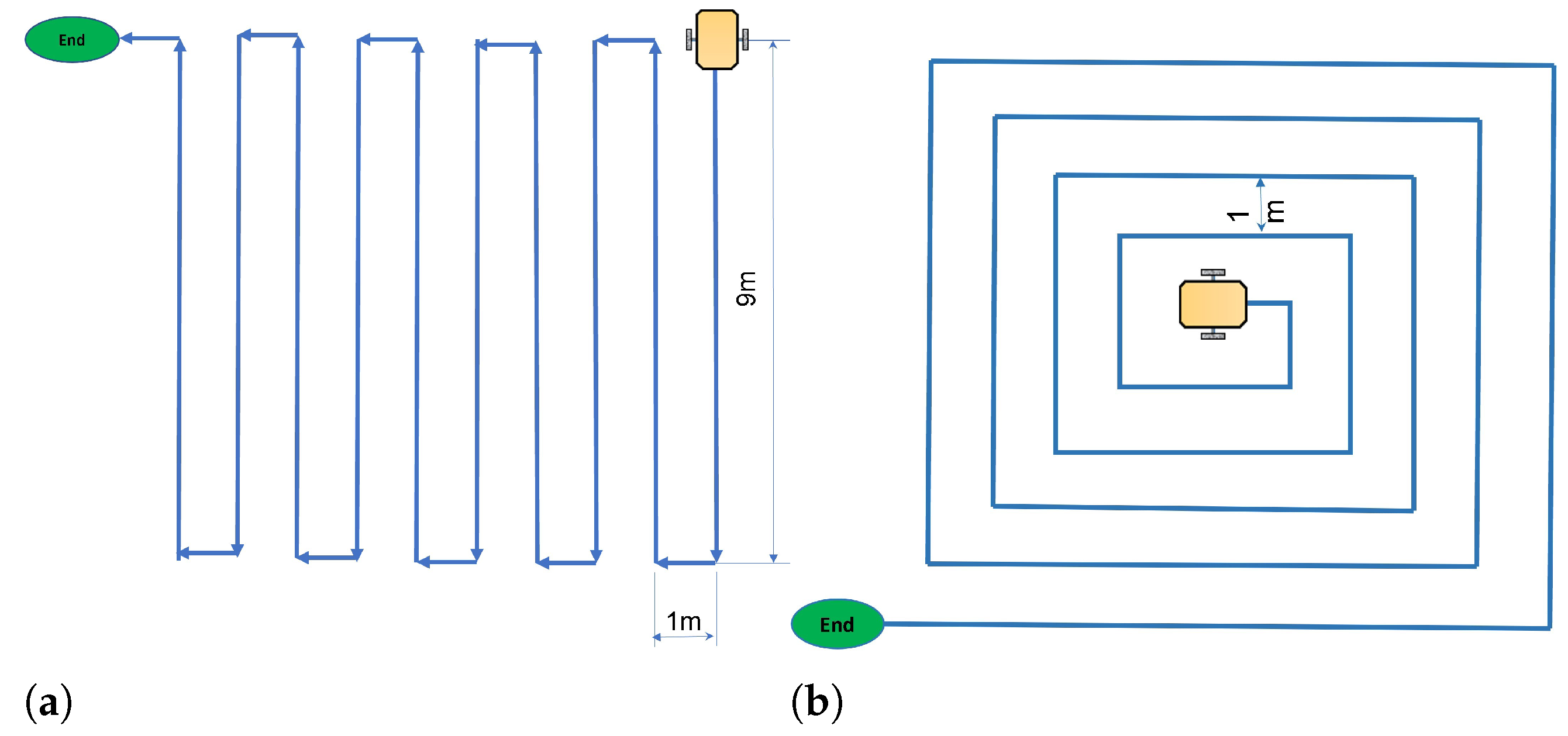
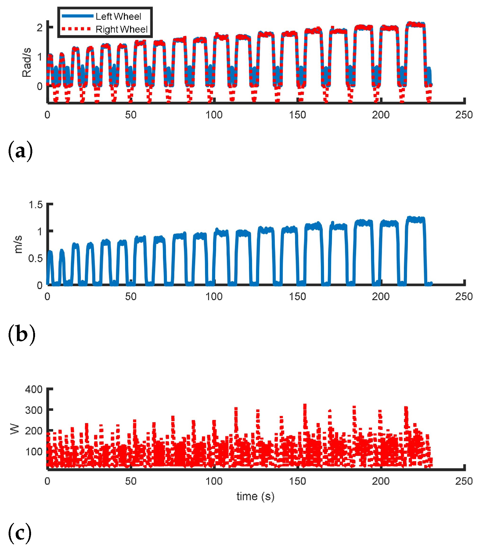
As highlighted above, the lack of standardized working cycles often leads to researchers developing their own cycles to suit their particular needs. In this regard, some typical working cycles need to be designed and conducted to powertrain designing and evaluating the hybrid electric AMR. Based on the typical characteristics of non-road vehicles such as AMRs, the driving cycle measurement has been considered the starting point. Subsequently, the basic AMR is moved using different velocities similar to typical real working cycles to measure the actual power requirement and energy consumption. In real farms, an AMR is usually employed in stop-and-go-loop working conditions. Therefore, we propose two typical pathways by considering the mixture of transitional and rotational movement patterns. 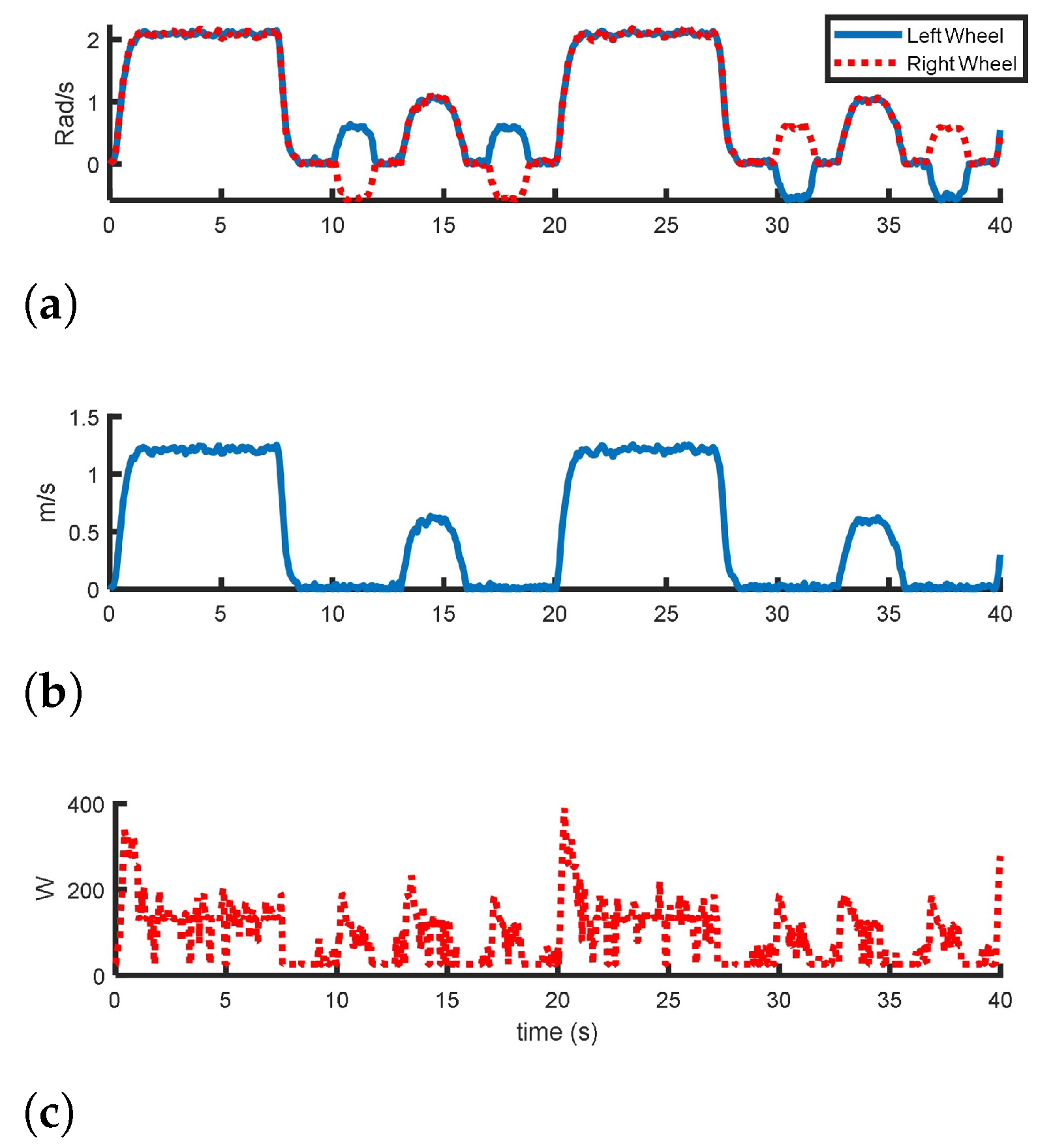They include row linear and perimeter circular movement patterns as shown in Figure 3. Each motion pattern was simulated for a 100 m distance and repeated three times in the same condition, considering a flat asphalt surface to minimize unexpected situations.

In addition, each test includes four sections, acceleration from stationary, constant velocities, and deceleration to stationary, then turning 90 degrees left or right. In this respect, the battery voltage and current, motor power, and velocity of the wheels are recorded by the developed data logger with a 0.1 s sample rate. The speed profile and the traction power required for completing the working cycles could be employed by a dynamic model in the designing process, such as estimating energy requirements, tuning energy management strategies, and component sizing.

2.4. The FCAMR Powertrain Modeling

As mentioned before, designing a hybrid electric AMR is a complex process and is usually constrained by time and budget. Therefore, model-based design is usually used as an engineer aid tool to simulate vehicles in a computer before construction. Some software such as ADVISOR [35], and Autonomie [36] are used in literature to simulate hybrid electric vehicle powertrain. However, they are not applicable directly in non-road vehicles and robots’ powertrain simulation due to specific powertrain architectures and features. In one of the authors’ previous works of the authors [23], a differential drive mobile robot powertrain model is presented and evaluated. Those details will not be repeated in this paper. Consequently, that model was modified for the energetic analysis of an FCAMR in this work. In this regard, a realistic MATLAB Simulink model is developed to simulate the hybrid FCAMR. Some fundamental aspects that are necessary to develop the PV/FCAMR powertrain are mentioned in the following sections. Figure 4a shows the free body diagram of the forces that interact with the AMR which will be described more in the next section. Figure 4b shows a schematic view of a differential drive AMR with two drive wheels and two castors that have been added for the vehicle balance. Each drive wheel could be rotated independently fore-and-aft. Subsequently, the robot’s trajectory can be determined by changing the drive wheels’ revolution.

2.4.1. Powertrain Model Evaluation

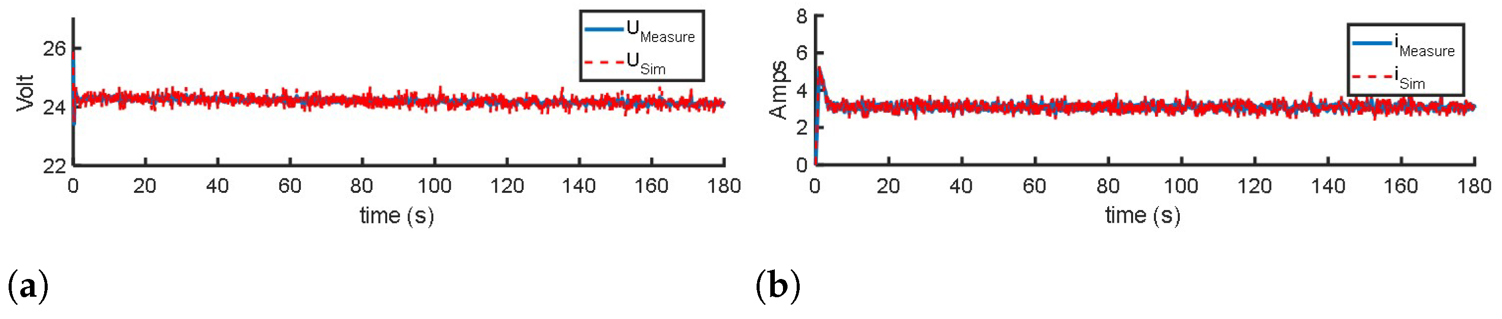
To evaluate the developed model, a comparative study in the first step is performed between the simulation results and the extracted experimental data by the basic battery-powered AMR. Therefore, the AMR is tested without a load while the wheels are off the ground to achieve full speed ($1.8$ m/s). This test has been conducted in order to eliminate surface effects on the performance of the AMR to assess model accuracy. Hence, the experimental data and simulation results for the vehicle when the environmental resistance and the vehicle weight are removed from the wheels are shown in Figure 5. Figure 5a compares the DC-bus instantaneous voltage from the real-world test and the simulation, and Figure 5b compares the consumed current by the motors. These results confirm an exact synergy (with an accuracy of 95%) between the energy model and the real battery-powered AMR performance.

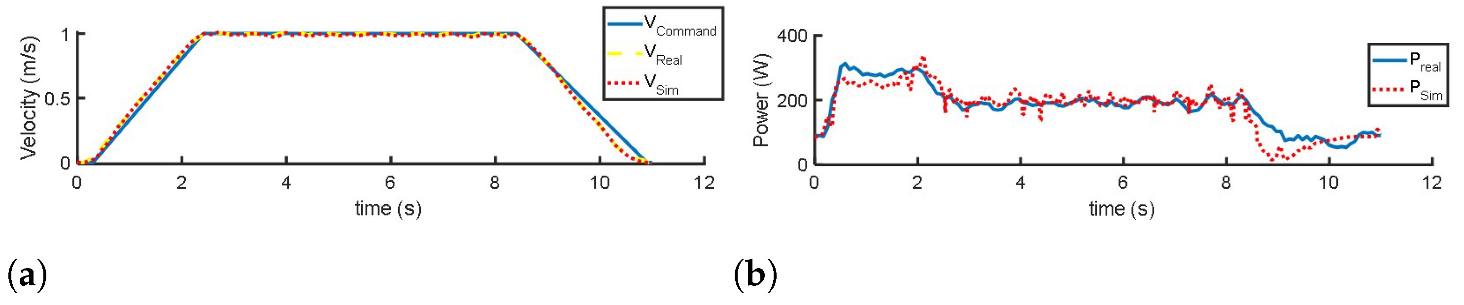
The actual power requirement and energy consumption using a trapezoid speed profile are compared with the result from the AMR Simulink model. In this regard, the maximum linear velocity in the trapezoidal speed profile scenario was considered as 1 m/s (Figure 6a). Similarly, the acceleration time from rest to maximum speed and vice versa was adjusted to two seconds to prevent high mechanical and electrical stresses. Figure 6b shows an adequate match between the measured power requirement based on the speed profile as a reference for the Simulink model and the obtained power requirement from the simulation. These results showed that the Simulink model has enough accuracy for energy estimation purposes for the rest steps of the hybrid AMR powertrain designing process.

2.4.2. Energy Requirements of Traction System

An AMR operates at a low speed in the field and mainly overcomes some forces such as rolling resistance, slope resistance, and acceleration resistance. The AMR also needs to overcome load resistance for agricultural tasks which distinguishes them from conventional vehicles. Thus, the total energy consumption ($E_{Tot.}$) connected to the AMR motion could be formulated as the following equation:

$$E_{Tot}=E_{res}+E_{Others}$$

(1)

where $E_{res}$, and $E_{Others}$ denote the energy needed to overcome the kinetic resistance forces, and energy losses by other accessories, such as sensors plus the actuators’ energy consumption, respectively. To obtain the required energy to drive the AMR during the given working cycle, it is necessary to consider vehicle dynamic behavior by calculating the opposite forces $F_{res}$ such as rolling $F_{roll}$, aerodynamic resistance $F_{air}$, and slope resistance $F_{hill}$ that prevent the movement. $E_{res}$ could be calculated using Equation (2) [23].

$$\begin{array}{cc}\hfill E_{res}& ={\int }_0^t\left(F_{roll}+F_{air}+F_{hill}\right)\mathrm{d}t\hfill \\ \hfill & ={\int }_0^t\left(C_{roll}·m·g\right)\mathrm{d}t\hfill \\ \hfill & +{\int }_0^t\left(\frac{1}{2}\rho ·A·C_{air}·{(V+V_w)}^2\right)\mathrm{d}t\hfill \\ \hfill & +{\int }_0^t\left(m·g·sin\alpha \right)\mathrm{d}t\hfill \end{array}$$

(2)

where $C_{roll}$ is the rolling resistance coefficient; g is the gravity acceleration; $\rho$, $C_{air}$, A, and $V_w$ are the air density, drag coefficient, frontal area, and wind velocity, respectively. $\alpha$ is the road or field slope. Rolling resistance can be modeled as a coefficient of friction which is reported in the range of coefficients expected on a farm [37].

Table 2. The main components specifications of the AMR.

Specification	Symbol	Value
Vehicle total mass	m	90 kg
Frontal area	A	0.7 m${}^2$
Aerodynamic drag coefficient	$C_{air}$	0.45
Air density	$\rho$	1.225 kg/m${}^3$
Wheel Radius (R)	R	0.096 m
Wheelbase	L	0.75 m
Rolling resistance coefficient	$C_{Roll}$	0.1
Gearbox ratio	$\xi$	16
Gravity acceleration	g	9.81 m/s

lists the main parameters that have been considered for modeling.

2.4.3. Initial Parameters of Energy Storage Subsystem

The total instant traction power required by the AMR is estimated to determine the batteries’ size. Then, the energy consumption was calculated to assess the characteristics of the energy storage system ($E_{Batt}$) using the measured working cycles and the Simulink model. An initial calculation can be performed by the following formula:

$$E_{Batt}=\frac{\Delta E_{Batt}}{SO{C}_{Final}-SO{C}_{Init}}$$

(3)

where $\Delta E_{Batt}$ is energy consumption, $SO{C}_{Final}$, and $SO{C}_{Init}$ denote the battery’s final and initial state of charge during the cycle, respectively. Based on the SOC curve, a $SO{C}_{Final}$ of 30%, and $SO{C}_{Init}$ equal to 100% are considered, which are representative values to prevent fast battery degradation. Consequently, battery pack capacity ($Q_{Batt}$) could be estimated as:

$$Q_{Batt}=\frac{E_{Batt}}{V_{Bus}}{\eta }_{Batt}·F$$

(4)

where $V_{Bus}$, ${\eta }_{Batt}$, and F represent the nominal voltage, efficiency, and charge factor of the battery. The battery’s efficiency is considered equal to 85% [38], and the charge factor guarantees to obtain the battery capacity at 1C is equal to 1.5. The SOC estimation of the battery is a fundamental parameter in electric vehicles. The physical model of the battery estimates the SOC using the Coulomb counting technique, which is a preferred way in EVs simulations. The technique consists of calculating the battery SOC ($SO{C}_{Batt}$) by measuring the current of the battery ($I_{Batt}$) and integrating it over time by the following expression [39,40]:

$$SO{C}_{Batt}=SO{C}_{Init}-\frac{100}{3600Q_{Batt}}{\int }_0^t{I}_{Batt}dt$$

(5)

2.4.4. Fuel Cell as a Range Extender

The FC is considered a voltage source based on its static polarization curve. In addition, the hydrogen flow rate is estimated based on experimental data by a linear function fitting, where a and b signify fitting parameters [41].

$${\dot{m}}_{H2}=a+b·i_{FC}$$

(6)

Consequently, the $H2$ cost can be calculated considering the total fuel consumption:

$$Cos{t}_{H2}=H{2}_{USD}{\int }_0^t{\dot{m}}_{H2}dt$$

(7)

To take into account the added onboard energy source, the $SOC$ of the $H2$ tank ($SO{C}_{H2-Tank}$) is calculated by the following equation:

$$SO{C}_{H2-Tank}=\frac{m_{H2-Init}-{\int }_0^t{\dot{m}}_{H2}dt·i_{FC}}{m_{H2-Init}}$$

(8)

Then, $m_{H2-Init}$ is the initial mass of $H2$ (g), ${\dot{m}}_{H2}$ is the $H2$ mass flow ($g/s$) and $i_{FC}$ is the FC current. A 300 W PEMFC parameters (FCS-C300 from Horizon Fuel Cell Technologies, Singapore) is considered as a base [42]. In addition, the FC system is composed of a DC-DC converter, a boost chopper, and a smoothing inductor for its current control. Their energetic performances are included in the FC static characteristics.

2.4.5. Photovoltaic System as an Energy Assistance

The PV system is considered a voltage source. In this regard, the onboard PV system with approximately 0.5 m${}^2$ (available surface on top of the FCAMR) acts as an energy assistant, shade, and protector. A 50 W peak power (Wp) could be generated using a monocrystalline panel [43]. The average amount of hourly available PV power in Trois-Rivieres, QC, Canada (latitude 46°20${}^{\prime }$49.7″ N, longitude 72°34${}^{\prime }$37.7″ W) is applied as the PV system model. This information can be obtained from the National Renewable Energy Laboratory website [43]. In eastern Canada, agricultural operations are usually performed from April to September. Therefore, the average hourly solar power in this period, is applied to the model as a lookup table. It should be noted that the FCAMR system has other components, such as sensors, microcontrollers, and other onboard electronic components, which are accessory parts. These components are extremely efficient nowadays but still consume a portion of the battery’s current. These components are modeled based on the data provided by the manufacturers in lookup table blocks. Subsequently, the current loss due to the electronic components is signified as $I_{Others}$. Kirchhoff’s current law is used to model the parallel connection among the battery pack, traction motors ($I_{TS}$), FC ($I_{FC}$) system, PV system ($I_{PV}$), and $I_{Others}$ as follows:

$$I_{Batt}=I_{TS}-I_{FC}-I_{PV}+I_{Others}$$

(9)

Once the mathematical model was developed, the final dynamic model for the vehicle and the respective simulations were obtained using MATLAB Simulink. Each model part was provided based on the manufacturer’s datasheets and experimental test results. The model allowed a comprehensive parametric study of sizing and performance evaluation of the hybrid powertrain to be analyzed. Consequently, the size of the electric motor, batteries, and FC system could be established based on the vehicle’s energy requirements by using rule-based and optimization-based methods. Moreover, the range-extender capacity (required power and fuel tank capacity) can be sized by considering the available energy of the onboard battery.

3. Component Sizing and Design Optimization

As mentioned above, the component selection and prototyping of a hybrid powertrain system for an AMR are problematic because of various design choices and constraints. Generally, an FCREx is a battery electric vehicle with an FC range extender. In the FCRExs architecture, the electric machine is usually sized to comply with vehicle performance requirements. The FC system power meets the requested continuous loads. Typically, the battery pack can support a road with a 15% grade for a specific speed and is sized to drive 50% of the daily driving range. The hydrogen storage is sized to extend the expected range [44]. However, in optimal component sizing, vehicle performance requirements and constraints must be satisfied at the same time. Literature consideration shows that a variety of optimization algorithms are available for HEV design [34]. A detailed review of component sizing methods can be found in [45]. One choice for component sizing of HEVs is the application of nature-inspired optimization techniques, such as evolutionary and swarm algorithms [46]. It has been demonstrated that those techniques are capable of finding the global optimum solutions, even if the solution domain is a large scale, highly nonlinear, constrained and complex [47]. For instance, a Genetic Algorithm (GA) was applied to the component sizing optimization of a fuel-cell-powered PHEV in [48]. In addition, an integrated Particle Swarm optimization (PSO) was used for the optimal powertrain component design of an FC locomotive application in [49]. The PSO is relevant considering its few optimization parameters, good accuracy, and short computation time compared to other optimization approaches. Its disadvantage is the selection of constant values for updating velocity. 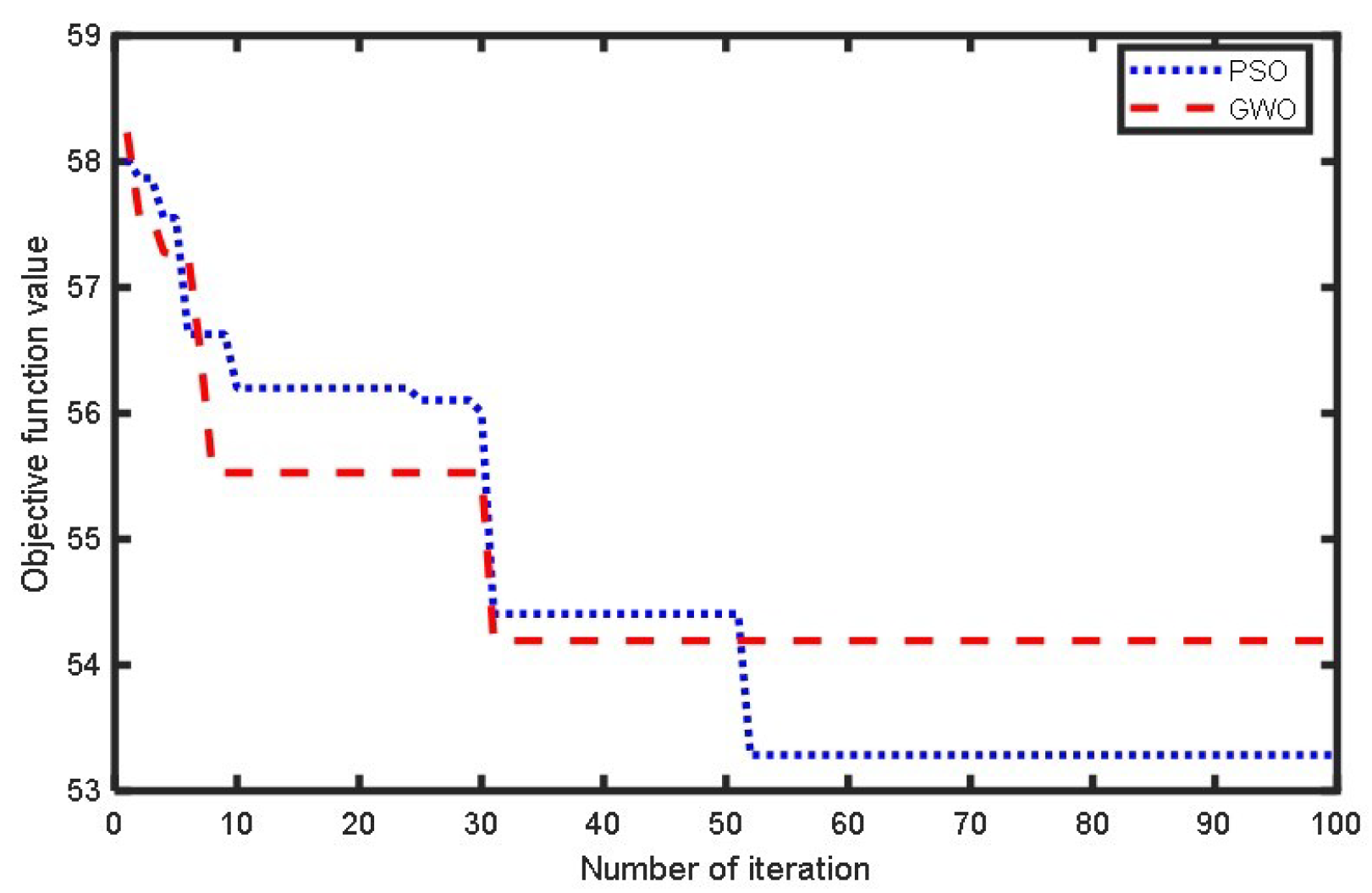If inappropriate constants are chosen, then the problem may not converge to the optimum [45]. However, there are other meta-heuristic based optimization methods such as Grey Wolf optimization (GWO) that was introduced recently and applied to the optimization in different fields. Therefore, the PSO is employed alongside of GWO to optimize the design parameters of the initial rule-based method. Consequently, the effects of the powertrain system and working cycle on component sizes are analyzed and compared. A brief description of both algorithms’ processes is given in the following sections.

3.1. Particle Swarm Optimization (PSO)

The idea of PSO came from the swarm intelligence found in many natural systems with group behavior. Ant colonies, bird flocks, and animal herds are a few examples of such natural systems. By considering an optimization function for the problem, PSO attempts to capture the global maximum or minimum value. More details about the optimization function and constraints are described in Section 3.3. The PSO algorithm follows some steps to solve an optimization problem. Firstly, the algorithm allocates initial random velocities and positions to all particles in space, the best particle of the particular ($pbest$), and the best particle of the swarm ($gbest$) to upgrade the position of each particle in turn [50]. The procedure is written as the following equations:

$$v_{i+1}=\omega v_i+c_1{r}_1(pbes{t}_i-x_i)+c_2{r}_2(gbes{t}_i-x_i)$$

(10)

$$x_{i+1}=v_{i+1}+x_i$$

(11)

where $c_1$ and $c_2$ are the cognitive and the social parameters which are considered 0.5 and 2.0, respectively. $r_1$ and $r_2$ are random numbers between 0 and 1. $\omega$ is the inertial weight equal to 0.8. Equation (10) gives the new velocity of the $i^{th}$ particle. Equation (11) determines the new position of the $i^{th}$ particle at each iteration. Particles are iteratively updated using these equations until an optimal solution is found or the number of iterations is reached. The number of iterations is set to 100, and the population set to 25.

3.2. Grey Wolf Optimization (GWO)

The Grey Wolf Optimizer is a metaheuristic algorithm originally developed by [51]. The GWO optimization method recreates the hunting behavior and leadership hierarchies of grey wolves. Based on the GWO algorithm, grey wolves live in packs at four levels of the hierarchy in nature. At the first level, there is a leader named alpha ($\alpha$); at the second level, there is the group beta ($\beta$); at the third level, the group delta ($\delta$); and the lowest-ranked group is omega ($\omega$). The grey wolves are characterized by a special group hunting technique including three principal phases including [52];

• Observe, race, and approach prey;
• Chasing, turning and provoking the prey until it stops;
• Attack on prey.

The hunting behavior of the grey wolves is modeled by a set of mathematical equations that can be implemented in numerical software tools. In the optimization algorithm, the prey is considered the optimal solution, and the wolves are considered the fittest solution. The wolves $\beta$ and $\delta$ represent the second and the third-best solutions, respectively, and the rest of the solutions are considered as the wolves $\omega$ that follow the other wolves during the hunt based on the optimization function and constraints (see Section 3.3). The mathematical model of the encircling phase is given as:

$$\begin{array}{c}\overrightarrow{D}=\left|\overrightarrow{C}\overrightarrow{Y_T}\left(k\right)-\overrightarrow{Y}\left(k\right)\right|\hfill \\ \overrightarrow{Y}(k+1)=\overrightarrow{Y_T}\left(k\right)+\overrightarrow{A}\overrightarrow{D}\hfill \end{array}$$

(12)

Then, k denotes the current iteration, $\overrightarrow{D}$ is the vector representing the distance between the prey and the wolf, $\overrightarrow{A}$ and $\overrightarrow{C}$ are coefficient vectors, $\overrightarrow{Y_T}$ is the prey position vector and $\overrightarrow{Y}$ indicates a grey wolf position vector. The exploration is guaranteed by A with random values proving the condition $\left|A\right|>1$ that assists the search agent to deviate from its prey. The exploitation (attack on the prey) starts when the condition $\left|A\right|<1$ is confirmed. This condition guarantees that the next agent position could be in a random location between the prey and its current position.

3.3. Model-in-the-Loop Optimization Process and Problem Definition

The approach for HEV design optimization is typically a model-in-the-loop design optimization process, as shown in Figure 7. The performance and design objectives, such as overall powertrain cost and fuel economy, can be evaluated using the vehicle model and computer simulation tools to design a hybrid powertrain for the AMR. Accordingly, using the design variables’ initial values, the vehicle model is simulated to obtain the numerical values of the objective function in the first step. At the same time, the constraint functions should be evaluated. These simulated results are then fed back into the optimization algorithm to produce a new set of values for the design variables. Then, the vehicle model is simulated again to achieve the values of the objective and constraint functions. The simulation results are fed back into the optimization algorithm to generate another new set of design variables. This iterative process repeats until the optimization process is finished. Note that the design variables remain within their limitation boundaries during this process.

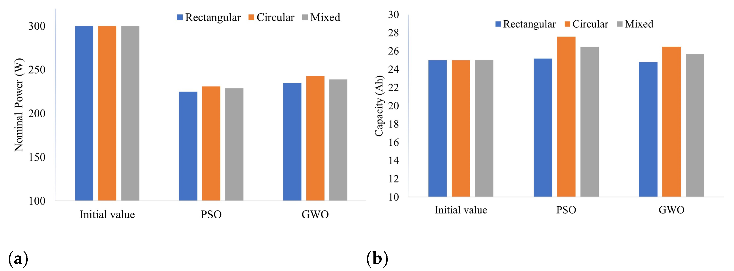
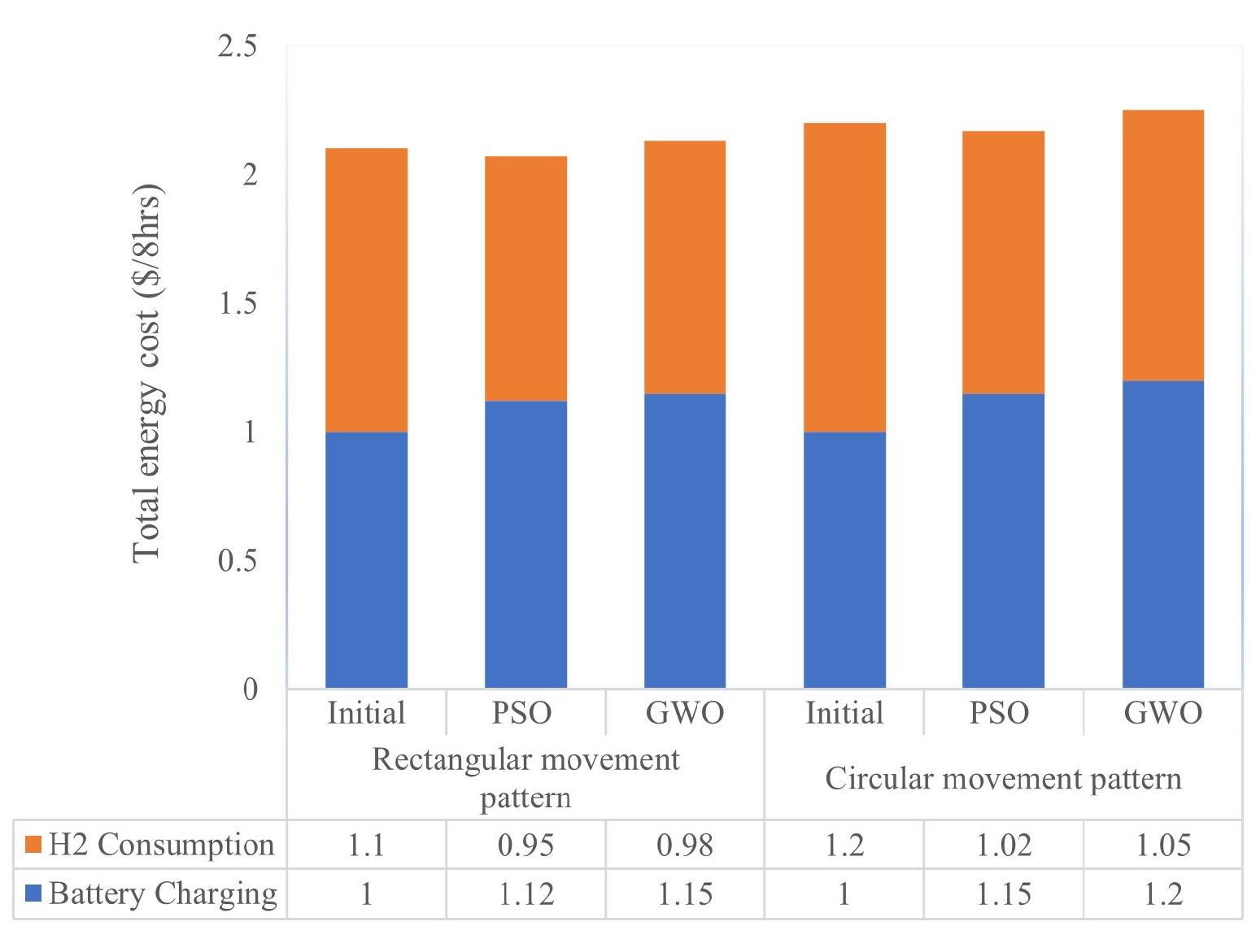
As a case study, the model in the loop has been programmed in MATLAB to optimize a PV/FCAMR for the overall vehicle powertrain cost on the extracted typical working cycles. The input variables including FC nominal power, battery capacity, hydrogen consumption, and electricity usage should be optimized. As the four input variables change, the vehicle model performs vehicle performance tests while checking constraints’ boundaries. The optimization process uses previous results to change the input parameters. A feedback process is then performed until the algorithm finds the optimal value for the objective function to find a trade-off relationship between FC and battery size.

Table 3. Initial design variables and boundary values for optimization.

Design	Initial	Lower	Upper
Variable	Value	Bound	Bound
FC power rating (W)	300	40	1000
Battery capacity (Ah)	24	3	40
Minimum SOC allowed (%)	30	20	40
Maximum SOC allowed (%)	90	80	100

shows the design variables used in this study with the boundary values. Accordingly, the optimization objective function (J) is defined to minimize powertrain cost of design variables, including the cost of the FC system ($C_{FC}$), battery ($C_{Batt}$), hydrogen ($C_{mH2}$), and electricity ($C_{Elec}$) [34,45] as following expressions:

$$\begin{array}{c}J=C_{FC}+C_{Batt}+C_{mH2}+C_{Elec}\hfill \\ C_{FC}=P_{FC}{\mathrm{Y}}_{FC}\hfill \\ C_{Batt}=Q_{Batt}{\mathrm{Y}}_{Batt}\hfill \\ C_{mH2}=m_{H2}{\mathrm{Y}}_{mH2}\hfill \\ C_{Elec}=E_{Elec}{\mathrm{Y}}_{Elec}\hfill \end{array}$$

(13)

where $P_{FC}$, $Q_{Batt}$, $m_{H2}$, and $E_{Elec}$ are the FC nominal power ($kW$), battery pack capacity ($Ah$), mass of hydrogen consumption ($kg$), and electrical energy consumption ($kWh$), respectively. ${\mathrm{Y}}_{FC}$, ${\mathrm{Y}}_{Batt}$, ${\mathrm{Y}}_{mH2}$ and ${\mathrm{Y}}_{Elec}$ are respectively the unitary cost of FC ($USD/kW$), batteries ($USD/Ah$), hydrogen ($USD/kg$), and electricity ($USD/kWh$).

The design constraints for both optimization methods are defined and bounded as follows:

$$\begin{array}{c}{P}_{FC-min}<P_{FC}\left(t\right)<P_{FC-max}\hfill \\ P_{Batt-min}<P_{Batt}\left(t\right)<P_{Batt-max}\hfill \\ SO{C}_{Batt-min}<SO{C}_{Batt}\left(t\right)<SO{C}_{Batt-max}\hfill \end{array}$$

(14)

where $P_{FC-min}$, $P_{FC-max}$,$P_{Batt-min}$, $P_{Batt-max}$, $SO{C}_{Batt-min}$, and $SO{C}_{Batt-max}$ are the minimum and maximum values of the FC power, the battery power, and the battery SOC, respectively. Control strategy parameters include SOC values. At the same time, the design problem’s constraints come from the following required vehicle performance:

• Maximum speed: 2 m/s;
• Maximum acceleration: 1 m/s${}^2$;
• Gradeability ≥15% (1 m/s).

It should be noted that the driving speed was limited to 2 m/s to avoid dangerous collisions between the mobile vehicle, workers, crops, etc. In addition, the maximum acceleration rate is limited to 1 m/s${}^2$ in order to use the electric motor at its higher efficiency region and to prevent high mechanical and electrical stresses on components.

3.4. Energy Management Strategy

When an FCAMR is being driven, the small-size range extender FC will provide power for the electric motors belonging to the battery. The batteries are charged when the vehicle is stopped. This task belongs to the EMS system of the hybrid electric powertrain. Two general control strategies, including charge depleting (CD) and charge sustaining (CS) could be used to determine the energy distribution of the FC and battery. In this work, a combination of these strategies is called the charge blending (CB) energy management strategy [23]. After its battery is fully charged, a PHEV operates in CD mode until its electric energy falls below the defined value, after which it switches to CS mode. The desired objectives in the CB mode include the following: the satisfaction of the power demanded by the motor driver and keeping the SOC as close as possible to the lowest safe level (20%) at the end of the working day. This strategy is suitable for applications where motion parameters (acceleration, velocity, slope, etc.) are the top priority for a low-speed vehicle with frequent stops and starts like an FCAMR. Since these control strategies are employed in the authors’ previous work [23] is not explained here again.

4. Results and Discussion

4.1. Working Cycle Evaluation

During the work of an AMR on a typical farm, there are several times of Stop and Go situations for avoiding obstacles and following the path. In addition, there are several times of rotating situations for finding the route. In large measure, the operating working range of an electric AMR depends on the working conditions, such as accelerations and decelerations at the beginning and end of the movement. Therefore, the obtained speed profile can be assumed as the typical behavior of a driver on the FCAMR working cycle. In this regard, several experimental tests have been conducted on a test bench in different scenarios and cycles based on their speed profiles from the experiment. In this article, an analysis of the AMR is performed on the two measured cycles described in the previous section to evaluate the proposed methodology.

Figure 8 shows the results of the rectangular working cycle pattern over time. Figure 8a illustrates a part of the angular velocity profile of the left and right wheels as a control command from the AMR control unit during driving in real conditions. The wheels have the same rotational speed while the robot runs in a straight direction. However, the wheels have different rotational directions when turning in the corners because of the deferential drive architecture of the AMR powertrain. These data result in the linear movement velocity profile of the AMR moving in the working cycle in Figure 8b. Consequently, from measured data (battery output current and voltage) by the data acquisition unit, the instant total power consumption could be calculated as shown in Figure 8c. Finally, total energy consumption can be estimated from the accumulated instantaneous power. As a result of estimating energy requirements in different scenarios, other design aspects such as component sizes, EMS performance, and battery SOC can be optimized.

In addition, Figure 9 shows the circular working cycle pattern with a different speed profile in the whole cycle. In these scenarios the AMR move in a circular path (as presented in Section 2.3). Therefore the diameter of the moving path increase during the test. Since the moving pattern differs from the rectangular one, its speed profile, power requirement, and energy consumption were obtained differently. Based on data obtained at the two typical working cycles, it should be noted that the maximum capacity of electric motors is rarely used. In fact, the drive system works most of the time in the partial load range. Note that, electric motors operate in several ranges of angular velocities and under different conditions, so their efficiency deviates from its maximum level. Thus, the fluctuation in power consumption could be occurred due to the various power requirements for acceleration, rolling resistance, and electric efficiency at different speeds.

Table 4. Measured parameters of the rectangular and circular movement pattern during the experiment.

	Rectangular	Circular	Standard
Parameters	Movement	Movement	Deviation
	Pattern	Pattern
Travel distance (m)	100	100	0
Time (s)	180	230	50
Average linear velocity (m/s)	0.56	0.43	0.13
Maximum linear velocity (m/s)	1.29	1.2	0.09
Average power requirement (W)	135.86	138.61	2.75
Maximum power requirement (W)	460.95	371.03	61.92
Number of rotational movements (N)	18	19	1
Total energy requirement (kJh)	6.79	8.86	2.06

shows the results from the measured working cycles. Both working cycles have the same travel distance of 100 m. Still, in the case of the circular movement pattern, around 50 s more time is needed to reach the final destination due to lower speed at short movement distance at the beginning and extra required rotational movement. The average linear velocity is $0.56$ m/s for the rectangular movement pattern compared with $0.43$ m/s for the circular one. However, the average power requirements for both of the working cycles are almost the same amount, while in the circular movement pattern, the robot needs to have one more rotation movement to reach its destination. These results demonstrate a higher energy consumption of $8.86$ kJh compared with $6.79$ kJh on the rectangular movement pattern with almost 2 kJh more energy requirements.

It should be noted that most agricultural work is performed repeatedly in certain rows with specific work patterns. Still, cyclical and random movements can occur in free working conditions and trajectory planning situations. Therefore, the measured data from both cycles are integrated (called mixed motion pattern) and used as a third working cycle in the simulation process.

4.2. Optimization Performance Evaluation and Working Cycle Effect on Components Size of the FCAMR

In order to evaluate the performance of the component sizing optimization process for the designed FCAMR powertrain, three working cycle scenarios, including circular, rectangular, and mixed movement patterns compared in terms of component sizing and fuel economy under the two different optimization methods. Subsequently, the GWO, and PSO are looped with the MATLAB and Simulink model, and the optimization is carried out as explained in the previous sections. Figure 10 shows how the objective function value improves versus the design iteration number in both optimization methods for the Mixed working cycle. The dashed curve is for the GWO case, and the dotted curve is for the PSO case. Fuel economy improvement with the GWO and PSO algorithms is very close until about 10 times function evaluations, after which GWO fall down of PSO until about 30. However, finally, the PSO catch the GWO. After about 30 function evaluations, the GWO did not find any good design point to get further improvement in the objective function value. However, the performance of PSO is improved to 50 iterations. Overall, PSO performed the best for this particular design optimization problem.

A comparison of the fuel economy before and after the optimization is given in

Table 5. Fuel consumption comparison between rule-based and optimization-based designing methods.

Working Cycle Movement Pattern	Fuel Consumption
	Before Optimization	After Optimization
		GWO	PSO
Rectangular	+55	+51	+50
Circular	+62	+58	+56
Mixed	+59	+54	+53

. In this regard, the AMR was primarily simulated based on initial parameters obtained by the rule-based method in the developed MATLAB Simulink model. The fuel economy for the initial rule-based method, PSO, and GWO was observed to be 55, 50, and 51 g on average for the rectangular movement pattern working cycle. Similarly, an average hydrogen consumption of around 62, 56, and 58 g is estimated for the circular movement pattern working cycle. Finally, approximately 59, 53, and 54 g in average hydrogen consumption are estimated for the mixed movement pattern working cycle, as given in the last row of Table 5. Essentially, all the optimization algorithms resulted in improved FCAMR fuel economy performance. A significant improvement (approximately 8 per cent) in the fuel economy is seen due to optimization (to a lesser extent in the case of the GWO compared to the PSO, though).

The optimization problems of the measured working cycles are solved to study the effect of a working cycle on the component sizing. The optimization results for the circular, rectangular, and mixed working cycles are compared with the initial values in Figure 11. Given the vehicle performance constraints, the trade-off of the FC and battery pack sizing can be realized by adjusting the lower and upper bounds of the design variables. Results showed that the rating of the FC power is significantly reduced, implying that the FC system has been downsized in all working cycle scenarios. For instance, the initial FC power for the mixed movement pattern obtained is approximately 229 W and 239 W in PSO and GWO, respectively. On the other hand, the battery is upsized to a greater extent of 26.5 and 25.7 Ah in the PSO and GWO cases to use more renewable energy-based electricity to be charged by the PV system. In addition, the circular pattern parameters show higher values than other working cycles due to the requirement of more stop-and-go conditions during the experimental test.

Table 6. PSO and GWO optimization results for the mixed working cycle.

Variable	Unit	Value
		GWO	PSO
FC nominal power	W	239	229
Battery Max Power	W	615	630
Battery Capacity	Wh	562	571
Hydrogen tank capacity	kg@ 300bar	0.15	0.15

summarizes optimal values of the design variables for the mixed movement working cycle for the FCAMR system. The simulation results indicated that the PSO could outperform the GWO for the component sizing problem. However, the difference was not obtained significantly for the mixed working cycle, which could be due to the similarity of their meta-heuristic theory origin from nature.

We assumed USD 16 as the hydrogen price per gasoline gallon equivalent (0.997 kg of H2) to calculate the energy cost. Component costs are considered based on the 2020’ automotive FC system price defined by the US Department of Energy [53]. Battery cost is estimated using energy and power, i.e., USD 570 for a 24 Ah 24 Volt lead acid battery pack, including charger. The FC system cost is calculated based on the peak power of the stack and the capacity for the tank based on the assumptions used to analyze fuel cell technology in 2018 [54].

4.3. Working Cycle and Optimization Effects on the FCAMR Energy Cost

In this section, the performance of the initial and optimized powertrain architecture in terms of equivalent energy cost is compared based on simulations. The bar chart in Figure 12 compares the total energy costs of each working cycle between initial and optimized powertrain components in 8 h. Details show that the consumed energy cost of circular movement patterns at the initial design parameters obtained a maximum of almost 2.32 USD per working day (8 h). By contrast, the PSO optimized powertrain architecture for the rectangular movement pattern consumed a minimum of 2.07 USD per working day. Results from the simulation indicate that more than half of energy costs in the initial and optimized powertrains are related to hydrogen consumption. However, in the optimization method, the system used more batteries than FC. Overall, the PSO and GWO optimization methods achieved around 10 and 8 percent less energy consumption, respectively, compared to the initial rule-based component sizing method for the FC range extender AMR.

It should be noted that considering the average power of the PV system and battery charger efficiency, approximately 800 Wh of renewable electrical energy is produced and used to charge the battery pack. This amount could save almost 0.8 USD per day.

4.4. Power Split between Power Sources on Different Working Cycles

Figure 13a presents the power flow of the optimal FCAMR system response, including the FC system, battery pack, PV system, and storage systems’ SOC, compared to the total power load during 8 h of working daytime. As can be seen, the hybrid drivetrain system is ensured by the hybrid power sources. Powers delivered in total $(P_{FC}+P_{Bat}+P_{PV})$ matches the total required power $P_{Tot}$. It can also be noticed from these figures that the load energy and power are effectively shared between the FC, battery, and PV system. The battery supplies the fluctuated content of the power requirement. The FC provides the lower dynamic component (after several minutes of start-up) and ensures the highest part of the required energy. The algorithm tries to use the FC in its most efficient range (nominal power) with less ON/Off switch. For instance, the FC starts and stops 5 times during the rectangular working cycle. Each time it was ON for approximately 1700 s. When the FC system is ON, the battery pack power consumption is less. It recharges when the driving demanded power is less than the FC and the PV systems’ generated power. The sources are, thus, well sized according to the load requirement.

The SOC trajectory (Figure 13b) tends to follow vehicle dynamic behavior and reaches the required final condition. The relevance of the sizing with respect to the energy storage systems’ capacity constraints is also verified through the battery SOC. The recommended final limits ($SO{C}_{Batt}\approx 0.4$ and $SO{C}_{H2-Tank}\approx 0.6$) are respected for the two storage systems. This demonstrates the effectiveness of the CB control strategy for finding the proper SOC values for both the battery pack and the hydrogen tank. Since the proposed hybrid powertrain architecture for the FCAMR is a PHEV, the initial SOC of the battery pack and the hydrogen tank is assumed to be 100% at the start of the day. The final Depth of Discharge (DOD) reached a reasonable level (0.7) for the battery. Therefore, the energy storage system (ESS) sizing results agree with the energy demand. The proposed design process fulfills the performance requirements under typical working cycles. It achieves an acceptable power splitting between the FC, battery and PV, thus, prolonging the continuous working time of the FCAMR.

These results are favorable and approve the aim of the arrangement to extend the vehicle’s autonomy with satisfactory performance under the tested situations so that it can work an entire day. The hydrogen that supplies power to the FC could be stored in a metallic hydrides tank with 0.15 kg H2, storage capacity at 300 Bars pressure. This tank extends the autonomy up to 15 h by incorporating a small-sized 225 W FC and 25 Ah lead acid battery pack without needing to charge the vehicle during the working day. Finally, these results have proven that using the proposed design process could be feasible for other vehicles with similar applications.

5. Conclusions

This article analyzed the energy behavior of an AMR as the preliminary step to developing a photovoltaic/fuel cell hybrid electric light-duty vehicle in the agriculture 5.0 concept. In this regard, an optimization-based process is proposed to design a PV/FC-powered AMR application. The experiments, simulations, and optimizations results show that:

• The FC system and battery pack size increased on working cycles with more rotational motion and stop-and-go situations. Therefore, the vehicle was less efficient, and the powertrain obtained higher cost in this working cycle. The drivetrain fuel consumption with a rule-based component sizing method is reduced by up to 12.21% compared to a PSO optimization-based method. The total cost of the PSO optimized powertrain was 8.79% lower than the one obtained by theoretical sizing method.
• Adding the PV system to the energy system increases the initial cost of the PV/FCAMR but slightly decreases the FC and battery pack size parameters. In addition, a PV system can extend the vehicle range by up to 5% and reduce fuel consumption costs by 7% compared to energy storage systems without PV.
• The proposed powertrain arrangement extends the autonomy of the basic pure electric system by 350% as opposed to the sole battery-powered system. This autonomy could allow the vehicle run for more than 10 h a day under the typical cycle with a hydrogen tank filled with 0.15 kg H2. The system studied in this research is a primary test bed for future works of the hybrid FCAMR in various applications such as seeding, spraying, and plant phenotyping. This technique could be used as a prototypical design strategy for other hybrid AMRs according to the customer’s needs.

The future perspective is that this kind of alternative energy-powered vehicle could be a feasible architecture for agricultural mobile robots applications as up-to-date renewable energy-based non-road vehicles. Furthermore, the software package for the autonomous guide and farm tasks will be designed to analyze the capabilities of the AMR in a real-world scenario in future studies.

References

1. Despoudi, S.; Sivarajah, U.; Dora, M. Definition of Agricultural Supply Chains and Sustainability Issues. In From Linear to Circular Food Supply Chains: Achieving Sustainable Change; Springer International Publishing: Cham, Switzerlands, 2021; Chapter 1; pp. 3–14. [Google Scholar] [CrossRef]
2. Rahman, M.M.; Khan, I.; Field, D.L.; Techato, K.; Alameh, K. Powering agriculture: Present status, future potential, and challenges of renewable energy applications. Renew. Energy 2022, 188, 731–749. [Google Scholar] [CrossRef]
3. Ghobadpour, A.; Monsalve, G.; Cardenas, A.; Mousazadeh, H. Off-Road Electric Vehicles and Autonomous Robots in Agricultural Sector: Trends, Challenges, and Opportunities. Vehicles 2022, 4, 843–864. [Google Scholar] [CrossRef]
4. Ghalazman, E.A.; Das, G.P.; Gould, I.; Zarafshan, P.; Rajendran, S.V.; Heselden, J.; Badiee, A.; Wright, I.; Pearson, S. Chapter 10—Applications of robotic and solar energy in precision agriculture and smart farming. In Solar Energy Advancements in Agriculture and Food Production Systems; Gorjian, S., Campana, P.E., Eds.; Academic Press: Cambridge, MA, USA, 2022; pp. 351–390. [Google Scholar] [CrossRef]
5. Kim, K.; Deb, A.; Cappelleri, D.J. P-AgBot: In-Row & Under-Canopy Agricultural Robot for Monitoring and Physical Sampling. IEEE Robot. Autom. Lett. 2022, 7, 7942–7949. [Google Scholar]
6. Gai, J.; Xiang, L.; Tang, L. Using a depth camera for crop row detection and mapping for under-canopy navigation of agricultural robotic vehicle. Comput. Electron. Agric. 2021, 188, 106301. [Google Scholar] [CrossRef]
7. Vibhute, A.S.; Tate Deshmukh, K.R.; Hindule, R.S.; Sonawane, S.M. Pest Management System Using Agriculture Robot. In Proceedings of the Techno-Societal 2020; Pawar, P.M., Balasubramaniam, R., Ronge, B.P., Salunkhe, S.B., Vibhute, A.S., Melinamath, B., Eds.; Springer International Publishing: Cham, Switzerlands, 2021; pp. 829–837. [Google Scholar]
8. Huang, C.H.; Chen, P.J.; Lin, Y.J.; Chen, B.W.; Zheng, J.X. A robot-based intelligent management design for agricultural cyber-physical systems. Comput. Electron. Agric. 2021, 181, 105967. [Google Scholar] [CrossRef]
9. Gao, X.; Li, J.; Fan, L.; Zhou, Q.; Yin, K.; Wang, J.; Song, C.; Huang, L.; Wang, Z. Review of wheeled mobile robots’ navigation problems and application prospects in agriculture. IEEE Access 2018, 6, 49248–49268. [Google Scholar] [CrossRef]
10. Raj, R.; Aravind, A.; Akshay, V.; Chandy, M.; Sharun, N. A seed planting robot with two control variables. In Proceedings of the 2019 3rd International Conference on Trends in Electronics and Informatics (ICOEI), Tirunelveli, India, 23–25 April 2019; pp. 1025–1028. [Google Scholar]
11. Sun, S.; Li, C.; Paterson, A.H. In-field high-throughput phenotyping of cotton plant height using LiDAR. Remote Sens. 2017, 9, 377. [Google Scholar] [CrossRef] [Green Version]
12. Jorgensen, R.; Sorensen, C.; Maagaard, J.; Havn, I.; Jensen, K.; Sogaard, H.; Sorensen, L. Hortibot: A system design of a robotic tool carrier for high-tech plant nursing. Agric. Eng. Int. CIGR Ejournal 2007, 9. [Google Scholar]
13. Ristorto, G.; Gallo, R.; Gasparetto, A.; Scalera, L.; Vidoni, R.; Mazzetto, F. A mobile laboratory for orchard health status monitoring in precision farming. Chem. Eng. Trans. 2017, 58, 661–666. [Google Scholar]
14. Green, O.; Schmidt, T.; Pietrzkowski, R.P.; Jensen, K.; Larsen, M.; Jørgensen, R.N. Commercial autonomous agricultural platform: Kongskilde Robotti. In Proceedings of the Second International Conference on Robotics, Associated High-Technologies and Equipment for Agriculture and Forestry: New Trends in Mobile Robotics, Perception and Actuation for Agriculture and Forestry, RHEA, Madrid, Spain, 21–23 May 2014; pp. 351–356. [Google Scholar]
15. Qiu, Q.; Fan, Z.; Meng, Z.; Zhang, Q.; Cong, Y.; Li, B.; Wang, N.; Zhao, C. Extended Ackerman Steering Principle for the coordinated movement control of a four wheel drive agricultural mobile robot. Comput. Electron. Agric. 2018, 152, 40–50. [Google Scholar] [CrossRef]
16. Aguiar, A.S.; dos Santos, F.N.; Cunha, J.B.; Sobreira, H.; Sousa, A.J. Localization and mapping for robots in agriculture and forestry: A survey. Robotics 2020, 9, 97. [Google Scholar] [CrossRef]
17. Iqbal, J.; Xu, R.; Sun, S.; Li, C. Simulation of an autonomous mobile robot for LiDAR-based in-field phenotyping and navigation. Robotics 2020, 9, 46. [Google Scholar] [CrossRef]
18. Oliveira, L.F.; Moreira, A.P.; Silva, M.F. Advances in agriculture robotics: A state-of-the-art review and challenges ahead. Robotics 2021, 10, 52. [Google Scholar] [CrossRef]
19. Xu, R.; Li, C. A review of high-throughput field phenotyping systems: Focusing on ground robots. Plant Phenomics 2022, 2022. [Google Scholar] [CrossRef]
20. Kumar, S.; Saket, R.; Dheer, D.K.; Holm-Nielsen, J.B.; Sanjeevikumar, P. Reliability enhancement of electrical power system including impacts of renewable energy sources: A comprehensive review. IET Gener. Transm. Distrib. 2020, 14, 1799–1815. [Google Scholar] [CrossRef]
21. Chambers, M.; Birney, C.; Young, B.; Ingwersen, W. Proof of Concept for a US Air Emissions Physical Flows Account. In Proceedings of the 37th Iariw General Conference, Paper 662. Lexington, MA, USA, 22–26 August 2022. [Google Scholar]
22. Li, M.; Bai, Y.; Zhang, C.; Song, Y.; Jiang, S.; Grouset, D.; Zhang, M. Review on the research of hydrogen storage system fast refueling in fuel cell vehicle. Int. J. Hydrogen Energy 2019, 44, 10677–10693. [Google Scholar] [CrossRef] [Green Version]
23. Ghobadpour, A.; Amamou, A.; Kelouwani, S.; Zioui, N.; Zeghmi, L. Impact of powertrain components size and degradation level on the energy management of a hybrid industrial self-guided vehicle. Energies 2020, 13, 5041. [Google Scholar] [CrossRef]
24. Rossi, C.; Pontara, D.; Falcomer, C.; Bertoldi, M.; Mandrioli, R. A hybrid–electric driveline for agricultural tractors based on an e-CVT power-split transmission. Energies 2021, 14, 6912. [Google Scholar] [CrossRef]
25. Ghobadpour, A.; Boulon, L.; Mousazadeh, H.; Malvajerdi, A.S.; Rafiee, S. State of the art of autonomous agricultural off-road vehicles driven by renewable energy systems. Energy Procedia 2019, 162, 4–13. [Google Scholar] [CrossRef]
26. Reddy, N.V.; Reddy, A.; Pranavadithya, S.; Kumar, J.J. A critical review on agricultural robots. Int. J. Mech. Eng. Technol. 2016, 7, 183–188. [Google Scholar]
27. Vaideeswaran, V.; Bhuvanesh, S.; Devasena, M. Battery Management Systems for Electric Vehicles using Lithium Ion Batteries. In Proceedings of the 2019 Innovations in Power and Advanced Computing Technologies (i-PACT), Vellore, India, 22–23 March 2019; Volume 1, pp. 1–9. [Google Scholar]
28. Castelli Dezza, F.; Musolino, V.; Piegari, L.; Rizzo, R. Hybrid battery–supercapacitor system for full electric forklifts. IET Electr. Syst. Transp. 2019, 9, 16–23. [Google Scholar] [CrossRef]
29. Cardenas, A.; Guzman, C.; Martinez, W. EV Overnight Charging Strategy in Residential Sector: Case of Winter Season in Quebec. Vehicles 2021, 3, 557–577. [Google Scholar] [CrossRef]
30. Noura, N.; Boulon, L.; Jemeï, S. A review of battery state of health estimation methods: Hybrid electric vehicle challenges. World Electr. Veh. J. 2020, 11, 66. [Google Scholar] [CrossRef]
31. Albarbar, A.; Alrweq, M. Proton Exchange Membrane Fuel Cells: Design, Modelling and Performance Assessment Techniques; Springer: Berlin/Heidelberg, Germany, 2017. [Google Scholar]
32. Fathabadi, H. Combining a proton exchange membrane fuel cell (PEMFC) stack with a Li-ion battery to supply the power needs of a hybrid electric vehicle. Renew. Energy 2019, 130, 714–724. [Google Scholar] [CrossRef]
33. Monsalve, G.; Ltaief-Belhaji, N.; Amoriya, V.; Cardenas, A. Kinematic Navigation Control of Differential Drive Agricultural Robot. In Proceedings of the CISTEM 2022—4th International Conference on Electrical Sciences and Technologies in Maghreb (CISTEM), Tunis, Tunisia, 26–28 October 2022. [Google Scholar]
34. Ehsani, M.; Gao, Y.; Longo, S.; Ebrahimi, K.M. Modern Electric, Hybrid electric, and Fuel Cell Vehicles; CRC Press: Boca Raton, FL, USA, 2018. [Google Scholar]
35. Turkmen, A.C.; Solmaz, S.; Celik, C. Analysis of fuel cell vehicles with advisor software. Renew. Sustain. Energy Rev. 2017, 70, 1066–1071. [Google Scholar] [CrossRef]
36. Taghavipour, A.; Vajedi, M.; Azad, N.L.; McPhee, J. A comparative analysis of route-based energy management systems for PHEVs. Asian J. Control. 2016, 18, 29–39. [Google Scholar] [CrossRef]
37. Andriaminahy, F.; Amamou, A.; Kelouwani, S.; Zioui, N.; Ghobadpour, A.; Agbossou, K. Comparative study of vehicle aerodynamic and rolling resistance coefficients estimation methods. In Proceedings of the 2019 IEEE Vehicle Power and Propulsion Conference (VPPC), Hanoi, Vietnam, 14–17 October 2019; pp. 1–5. [Google Scholar]
38. Iclodean, C.; Varga, B.; Burnete, N.; Cimerdean, D.; Jurchiş, B. Comparison of different battery types for electric vehicles. In Proceedings of the IOP Conference Series: Materials Science and Engineering; IOP Publishing: Bristol, UK, 2017; Volume 252, p. 012058. [Google Scholar]
39. Meng, J.; Luo, G.; Ricco, M.; Swierczynski, M.; Stroe, D.I.; Teodorescu, R. Overview of lithium-ion battery modeling methods for state-of-charge estimation in electrical vehicles. Appl. Sci. 2018, 8, 659. [Google Scholar] [CrossRef] [Green Version]
40. Monsalve, G.; Cardenas, A.; Martinez, W. SoC Estimation Techniques for Efficient Agricultural Robots. In Proceedings of the IECON 2021—47th Annual Conference of the IEEE Industrial Electronics Society, Toronto, ON, Canada, 13–16 October 2021; pp. 1–7. [Google Scholar]
41. Hissel, D.; Turpin, C.; Astier, S.; Boulon, L.; Péra, M.C.; Jemei, S. A Review on Existing Modeling Methodologies for PEM Fuel Cell Systems. In Proceedings of the Fundamentals and Development of Fuel Cells, FDFC’08, Nantes, France, 23–27 April 2008; pp. 1–6. [Google Scholar]
42. Horizon. Horizon-Pem-Fuel-Cell-h-300-Manual. Available online: https://www.fuelcellstore.com/manuals/horizon-pem-fuel-cell-h-300-manual.pdf (accessed on 24 November 2022).
43. NREL. PVWatts Calculator. Available online: https://pvwatts.nrel.gov/pvwatts.phpl (accessed on 25 August 2022).
44. Marcinkoski, J.; Vijayagopal, R.; Kast, J.; Duran, A. Driving an industry: Medium and heavy duty fuel cell electric truck component sizing. World Electr. Veh. J. 2016, 8, 78–89. [Google Scholar] [CrossRef] [Green Version]
45. Huang, Y.; Wang, H.; Khajepour, A.; Li, B.; Ji, J.; Zhao, K.; Hu, C. A review of power management strategies and component sizing methods for hybrid vehicles. Renew. Sustain. Energy Rev. 2018, 96, 132–144. [Google Scholar] [CrossRef]
46. Mozaffari, A.; Vajedi, M.; Chehresaz, M.; Azad, N.L. Multi-objective component sizing of a power-split plug-in hybrid electric vehicle powertrain using Pareto-based natural optimization machines. Eng. Optim. 2016, 48, 361–379. [Google Scholar] [CrossRef]
47. Wei, C.; Hofman, T.; Ilhan Caarls, E.; van Iperen, R. A review of the integrated design and control of electrified vehicles. Energies 2020, 13, 5454. [Google Scholar] [CrossRef]
48. Jain, M.; Desai, C.; Kharma, N.; Williamson, S.S. Optimal powertrain component sizing of a fuel cell plug-in hybrid electric vehicle using multi-objective genetic algorithm. In Proceedings of the 2009 35th Annual Conference of IEEE Industrial Electronics, Porto, Portugal, 3–5 November 2009; pp. 3741–3746. [Google Scholar]
49. Sarma, U.; Ganguly, S. Determination of the component sizing for the PEM fuel cell-battery hybrid energy system for locomotive application using particle swarm optimization. J. Energy Storage 2018, 19, 247–259. [Google Scholar] [CrossRef]
50. Tu, J.; Bai, Z.; Wu, X. Sizing of a Plug-In Hybrid Electric Vehicle with the Hybrid Energy Storage System. World Electr. Veh. J. 2022, 13, 110. [Google Scholar] [CrossRef]
51. Mirjalili, S.; Mirjalili, S.M.; Lewis, A. Grey wolf optimizer. Adv. Eng. Softw. 2014, 69, 46–61. [Google Scholar] [CrossRef] [Green Version]
52. Mirjalili, S.; Aljarah, I.; Mafarja, M.; Heidari, A.A.; Faris, H. Grey wolf optimizer: Theory, literature review, and application in computational fluid dynamics problems. In Nature-Inspired Optimizers; Studies in Computational Intelligence; Springer: Cham, Switzerland, 2020; pp. 87–105. [Google Scholar]
53. Miller, E.L.; Thompson, S.T.; Randolph, K.; Hulvey, Z.; Rustagi, N.; Satyapal, S. US Department of Energy hydrogen and fuel cell technologies perspectives. MRS Bull. 2020, 45, 57–64. [Google Scholar] [CrossRef]
54. Stephens, T.; Birky, A.; Gohlke, D. Vehicle Technologies and Fuel Cell Technologies Office Research and Development Programs: Prospective Benefits Assessment Report for Fiscal Year 2018r; Report; Argonne National Lab.(ANL): Argonne, IL, USA, 2017. [Google Scholar]
Figure 1. The hardware structure of studied AMR; (a) The preliminary design, (b) 3D model of the future platform.
Robotics 12 00013 g001
Figure 2. Proposed configuration of the hybrid electric PV/FCAMR platform.
Robotics 12 00013 g002
Figure 3. Testing routes; (a) Row linear movement pattern (b) Perimeter circular movement pattern.
Robotics 12 00013 g003
Figure 4. Differential drive AMR schematic model (a) Free body diagram, and (b) Kinematic diagram.
Robotics 12 00013 g004
Figure 5. Comparison results between experimental data and simulations: (a) instantaneous voltage of the DC-bus, (b) current by traction motors.
Robotics 12 00013 g005
Figure 6. Comparison results of experimental data from real AMR versus the developed Simulink model by trapezoidal speed profile, (a) velocity, and (b) power demand.
Robotics 12 00013 g006
Figure 7. Model-in-the-loop design optimization process.
Robotics 12 00013 g007
Figure 8. Obtained results for the measured speed profile during the rectangular movement pattern working cycle by the AMR in one round (20 m), (a) Wheels angular velocity (control command), (b) AMR linear velocity, (c) Instant traction power.
Robotics 12 00013 g008
Figure 9. Obtained results for the measured speed profile during the circular movement pattern working cycle by the AMR in one cycle (100 m), (a) Wheels angular velocity (control command), (b) AMR linear velocity, (c) Instant traction power.
Robotics 12 00013 g009
Figure 10. Performance comparison of PSO and GWO optimization versus the design iteration number for the FCAMR in a mixed working cycle (circular + rectangular movement pattern).
Robotics 12 00013 g010
Figure 11. Comparison of the FCAMR initial and optimized design variable values for different working cycles, (a) FC nominal power (W), and (b) Battery nominal capacity (Ah).
Robotics 12 00013 g011
Figure 12. Working cycles cost comparison for recharging the battery pack and hydrogen consumption by FC system.
Robotics 12 00013 g012
Figure 13. Results of (a) Instant power of the battery pack, FC system, and PV system compared to the total load requirement, and (b) Battery SOC and hydrogen tank SOC, for the final PSO optimized FCAMR case during 8 h working daytime.
Robotics 12 00013 g013