1. Introduction
Robotic manipulators are extensively being used in different areas such as the manufacturing industry, process and mining, automatic surgery, as well as smart agriculture [
1,
2]. These robots considerably reduce human effort in complex task operations by adopting different controllers [
3,
4,
5]. Despite the available control technologies in the state-of-the-art, there are still some gaps and unaddressed challenges in this domain. From the system modeling perspective, the Lagrange method is commonly used to model rigid-link manipulators [
6]. However, these multivariable systems are highly coupled and nonlinear, meaning that an accurate model representation is hardly obtained for such systems [
7,
8]. These issues can accommodate by designing a reliable controller that satisfies precision, fast-response rate, robustness, and adaptiveness properties by which the uncertain dynamics and disturbances are handled properly.
In the state-of the-art, the conventional SMC and its developments have been investigated for robotics and nonlinear systems control for several decades. To achieve acceptable systems performance, in [
9], a disturbance-observer-based SMC controller is developed for space manipulators with prescribed performance. Generally, the prescribed performance control (PPC) is an approach for ensuring the desired transient and steady-state system responses. This approach is associated with many challenges such as the time response and the initial error dependency, which can be developed in various ways [
10]. Furthermore, additional solutions are required for unpredictable perturbations [
10]. These challenging issues are well-handled with the stability proof in [
9]. In addition to PPC, the Barrier Lyapunov Function (BLF) method with the commonly Logarithm structure is used to satisfy a constrained control problem. Both BLF and PPC can be used to address time-variant constraints, while PPC is more convenient in mathematical differentiating operations. Moreover, PPC is less sensitive to the initial output error [
11]. Using these approaches, the system model is usually required in the control design. As an effective solution, neural network (NN)-based techniques are combined with BLF and PPC to estimate dynamical equations and model uncertainties [
12]. Regarding NN approaches, the inputs are required to be located on proper compacts set to lead to an effective estimation [
12]. Thus, the combination of an NN method with BLF and PPC is regarded as a promising strategy in the control domain. Generally, the neural networks-radial basis function (NNRBF) method is established by minimizing a quadratic cost function, however, it provides local optimization with a relatively slow convergence rate for obtaining the adaptive NN weights [
13]. In [
12], NNRBF is used as a neural estimator, applying the persistent excitation condition to improve the estimation. Different solutions are available to promote a learning-based estimation, and the ELM could be an alternative approach which is not extensively investigated [
14,
15].
As a recent neural technique, ELM is adopted in various control design frameworks including the SMC controllers [
14,
15,
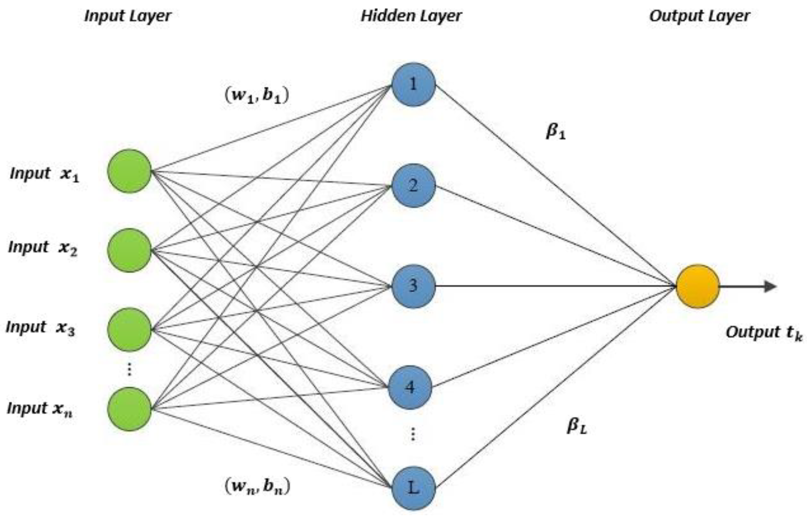
16]. Regarding the basic principles of ELM, NN weights are updated through single-hidden layer feedforward networks, and are more likely to converge with the global solution [
17]. The weights between the input and hidden layers are frozen by random values, which in part, increase the operation speed. Moreover, this type of value assignments, or in other words, random initialization, results in the universal approximation capability. This is the main rational behind the superior convergence capability of ELM over the NNRBF [
13]. Although, the output weights in ELM are generally computed by the least square optimization approach, in several studies, these parameters are obtained based on establishing the global stability [
18,
19]. Regarding the advantages of ELM, this method has been applied in different applications successfully, being proved as a promising approach in robotics and control [
20,
21,
22].
Similar to PP, the SMC control usually requires proper model description of a system. To address this problem, in [
23,
24], system uncertainties are estimated by NNRBF through the SMC approach. Regarding the prominent features of SMC, the combination of this method with PPC has been recently developed for different systems [
25,
26,
27] which drives the control system towards a robust performance with desired transient and the steady-state responses. In addition, fast system response is highly demanding in various robotics applications. This property is attained via the finite-time stability that should be mathematically proven in the design phase. This criterion is investigated for the neural sliding mode control approaches in [
28,
29].
Motivated by the above gaps and challenges, this paper proposes a finite-time trajectory tracking controller for a robotic manipulator system subject to parametric system uncertainties which ensures several performance criteria such as robustness, precision in tracking, and finite-time responses. The main contributions of this paper are as follows:
- (1)
Transient response of the system including overshoot/undershoot as well as the steady-state response including the fast convergence of the steady-state error is set in the design procedure. Moreover, the finite-time stability proof of the designed sliding surface and the error transformation is provided.
- (2)
ELM is used to overcome the difficulties in obtaining the precise model of the robot stemming from dynamic coupling effects, time-varying parameters, and nonlinear frictions. Although, SMC is robust against uncertainties, such effects could result in chattering phenomenon and the higher magnitude of the input torques. Thus, the ELM estimation is used to tackle this problem.
The rest of this paper is organized as follows. The mathematical model of robotic manipulators and some technical preliminaries are given in
Section 2. The design control procedure is presented in
Section 3. The stability of the proposed controller as well as the finite-time convergence rates is demonstrated in
Section 4. The performance of the controller is illustrated and analyzed by bringing the simulation results in
Section 5. Finally, conclusion and future work statements are pointed out in
Section 6.
4. Stability Analysis
Theorem 1. Consider a robotic manipulator described by (1). Design the control input (9) and the estimator (10). Then, the following objectives are achieved:
1. The closed-loop system is stable and all signals are bounded. Furthermore, model uncertainty is estimated with a stable learning process.
2. The sliding surface converges to zero within a finite time. The convergence speed towards the sliding surface can be regulated by the proper selection of the initial states and the design control parameter .
3. The prescribed performance is achieved with a rapid convergence rate. The error tracking converges to zero within a finite time. The convergence speed towards the prescribed performance, i.e., the settling time, can be regulated by the initial states and the design parameter .
Proof: The Lyapunov principle is used to prove Theorem 1. First, the sliding mode controller using the ELM-based estimation is proven to be asymptotically stable. Second, it is proven that the sliding surface reaches zero in finite time. The third part proves the rapid convergence of the error transformation.
A positive definite Lyapunov function is defined as (12).
By taking the time-derivative of (12), and using (8)–(11), it is easy to show that
Therefore, (), all signals are bounded, and the closed-loop system is asymptotically stable.
- 2.
Next,
is defined as follows:
According to Property 1,
, and take the time-derivative of (17), and replace (8) and (9) into it, gives:
Thus, the inequality is deduced ( is a matrix with activation function elements, thus, it can be selected with bounded functions upper-bounded as ).
Considering (20), is obtained, in which . Hence, the sliding surface moves toward zero within a finite time () as complies with (2). This indicates that depends on and .
- 3.
Considering (16) and (20), the sliding surface reaches zero as
. Thus, the following equation is obtained.
Finally,
is defined as follows:
Taking the time-derivative of (22) and replacing (21), yields:
According to (23), is deduced, considering (2),the prescribed performance is obtained and the error transformation converges to zero less than a determined time () as given in (3).
Regarding and , it is concluded that the proposed controller is exponentially stable within a finite time, while the PPC objective is satisfied. □
Remark 2. In this study, ELM is used to estimate model uncertainty based on the Lyapunov (the closed-loop stability) approach. Since this estimator consists of nonlinear activation functions in hidden layers, it is a proper choice to estimate uncertainties which are naturally nonlinear. In addition, the estimation of the upper bound of uncertainties is a challenging issue, and the improper selection of this parameter imposes negative impacts on the chattering phenomenon and, accordingly, system stability. Thus, this application of ELM is effective to alleviate this problem. Moreover, since ELM provides global estimation with a fast convergence rate, the combination of this technique with the proposed finite-time controller is realizable and applicable in practice.
Remark 3. Equation (21) is differentiable with a discontinuous right-hand side. Knowing that the classical sign function is not necessarily equal to zero when x = 0. Especially, when differential inclusions are involved. Under the Filippov principle, this challenging issue will be handled, and the classical sign function can be treated as a set-valued function [31]. Therefore, a modified sign function is required. Remark 4. According to (23), the error transformation reaches zero and the intended prescribed performance () is achieved exponentially with the convergence rate faster than . According to this deduction, is dependent on and , indicating that the settling time can be adjusted by the appropriate selection of the gain . This statement is valid as long as the initial conditions are correctly set within the prescribed boundary.
Remark 5. Regarding the system with the dynamic representation (1), and the assumption , if the sliding surface is chosen as , the control input is obtained as when the mentioned method is employed. This control design results in a finite-time stable control system with bounded signals. Also, the respective Lyapunov function leads to as it does have the form of (2). However, it does not verify that the PPC condition is achieved within a finite time because it results in . Regarding the proposed sliding surface , not only the sliding surface converges to zero within a finite time, but also it guarantees that the PPC objective is satisfied.
5. Simulation Results
In this section, the performance of the proposed controller is investigated via extensive simulation studies and under different operating conditions. The robot manipulator system is selected as a 2 degree-of-freedom (DOF) planar robot manipulator with the standard representation as given in (1). The following matrixes are used in this study [
32]:
where
are constant parameters dependent on the robot’s physical structure. The gravitation constant is defined as
, and the other elements are
[
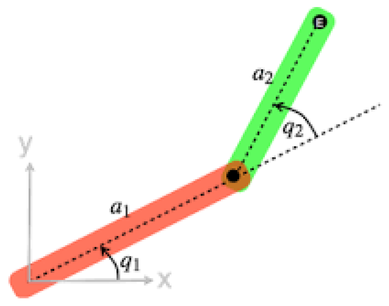
32]. According to
Figure 3, this robot consists of two links
, and two joints with angular outputs
. In which, each joint has 1-DOF, and the input torques are given to these joints.
As for a comprehensive evaluation, the performance of proposed controller is investigated under normal and uncertain operating conditions as well as a comparative study. In addition, the performance indices of integral absolute error as , integral time absolute error as , and the root-mean-square value of input torques as ( the step time, the total run time) are used for the numerical performance analysis. The simulations of this study were performed with MATLAB®2020a operated on a PC with an Intel i7 3.20 GHz quad-core processor.
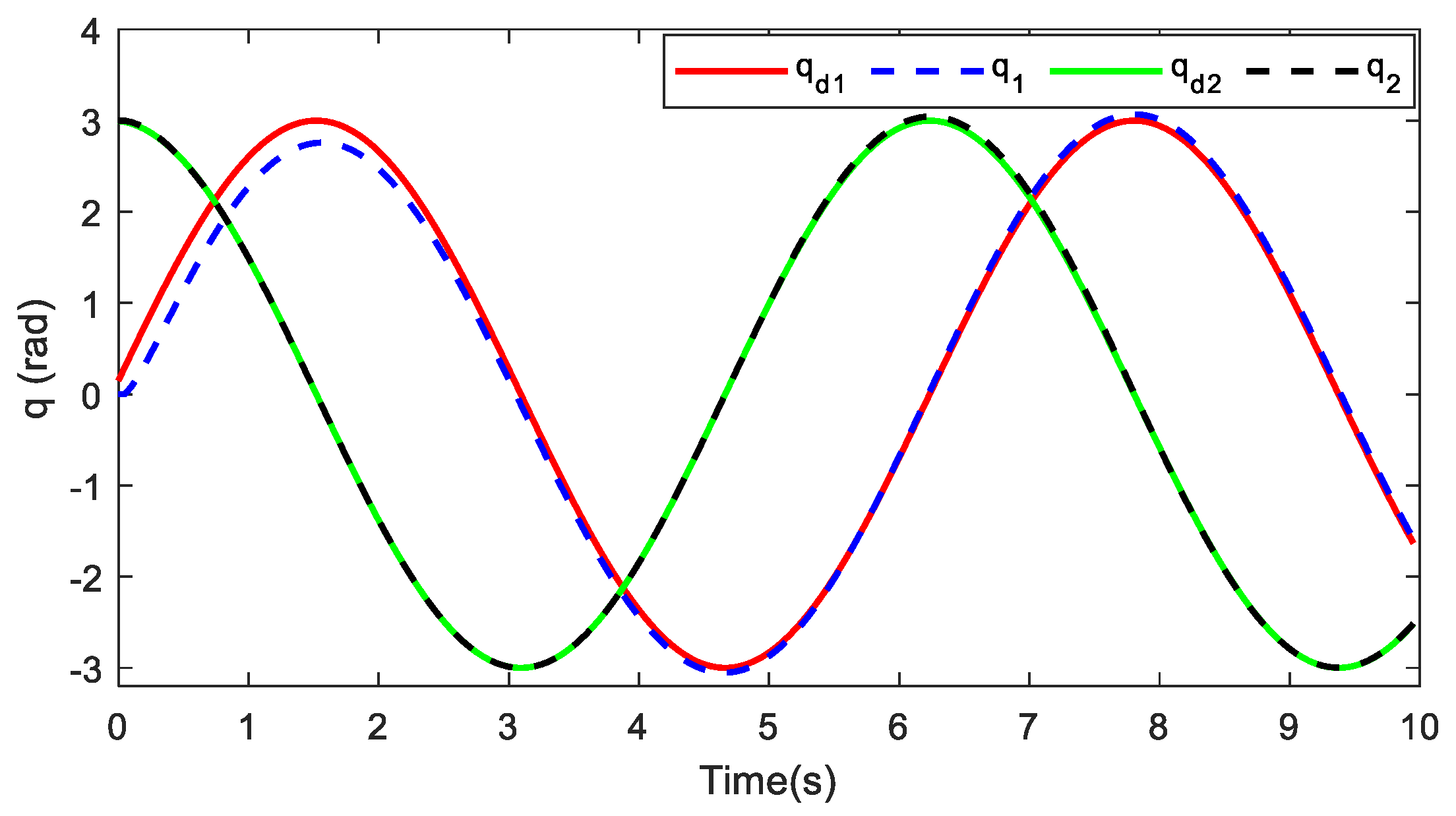
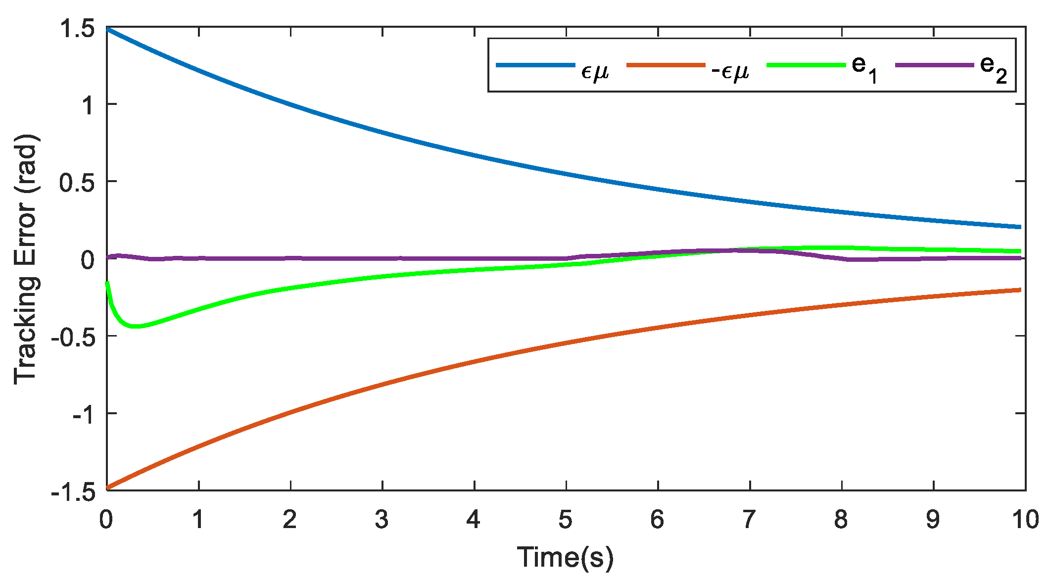
Scenario 1. Performance assessment under normal condition
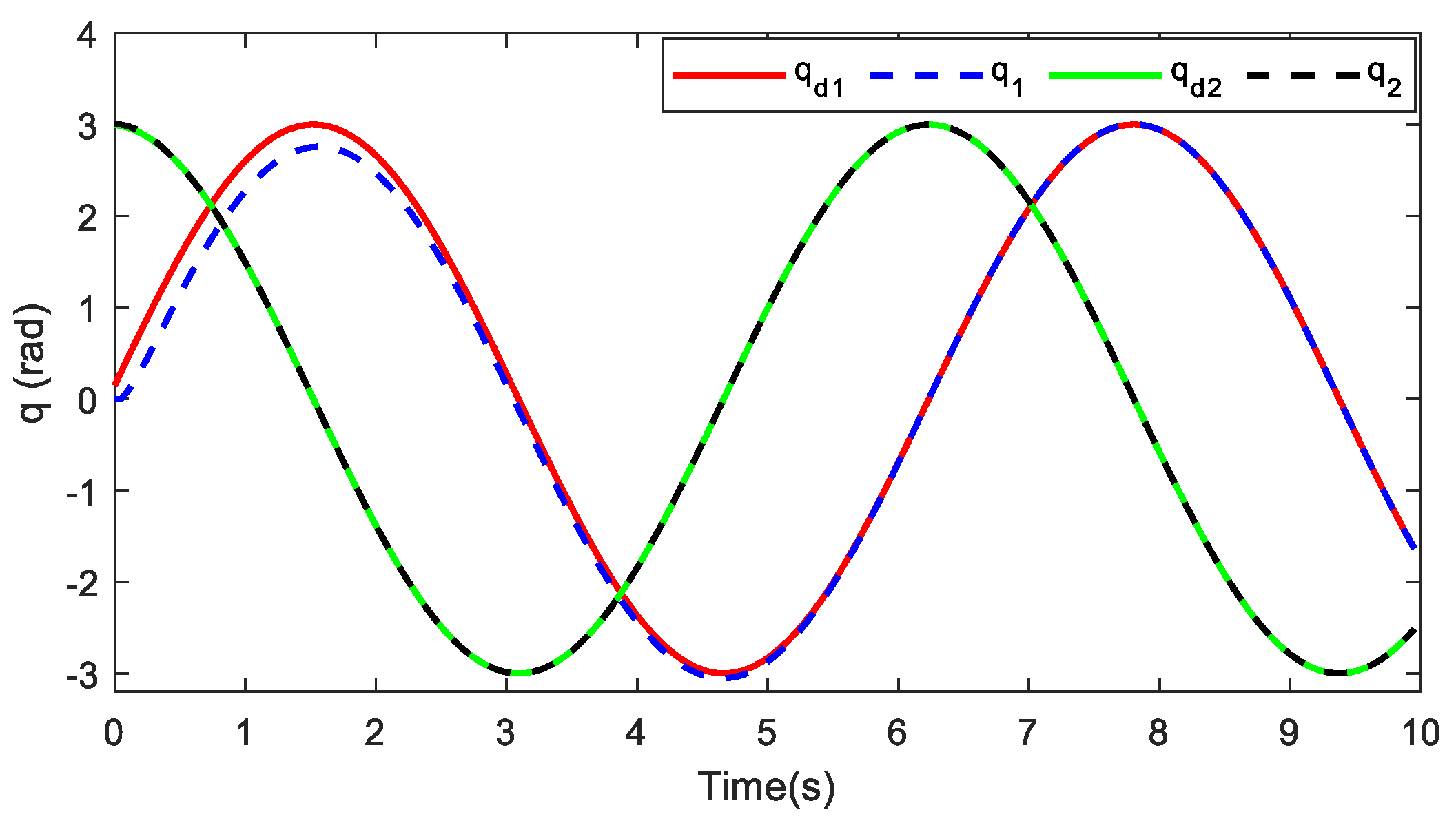
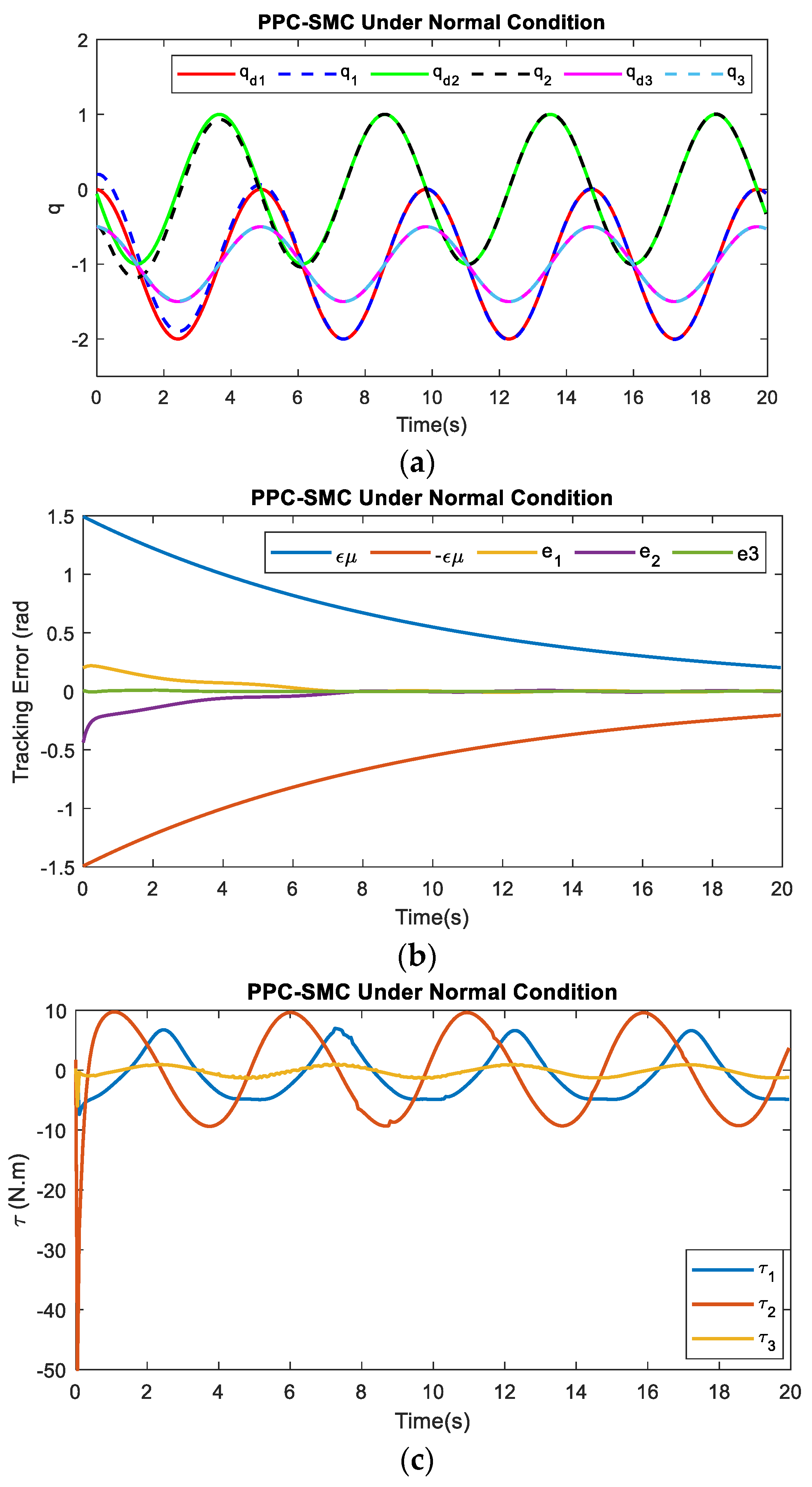
In this scenario, the reference tracking of the manipulator (24) is investigated via PPC-SMC and PPC-ASMC controllers, under normal operating condition (without model uncertainties). The reference signal for each joint is given as . The prescribed function is set as . The SMC parameters are selected as . The initial state for each joint is set as , which is located in an acceptable region.
Figure 4,
Figure 5 and
Figure 6 show the results of trajectory tracking obtained via PPC-SMC controller. According to
Figure 4,
Figure 5 and
Figure 6, the control law (9) performs well in reference tracking. Inferred from
Figure 4 and
Figure 5, the error tracking is small enough and it is drawn within the prescribed region, indicating that the overshoot and the steady-state error are obtained within the predetermined bounds. Thus, the convergence rate is faster than the prescribed function. It is inferred that all these conclusions are obtained within a finite time as follows:
,
(
).
Figure 6 indicates that the input torque for each joint is obtained with an acceptable amplitude, and it does not have the chattering problem.
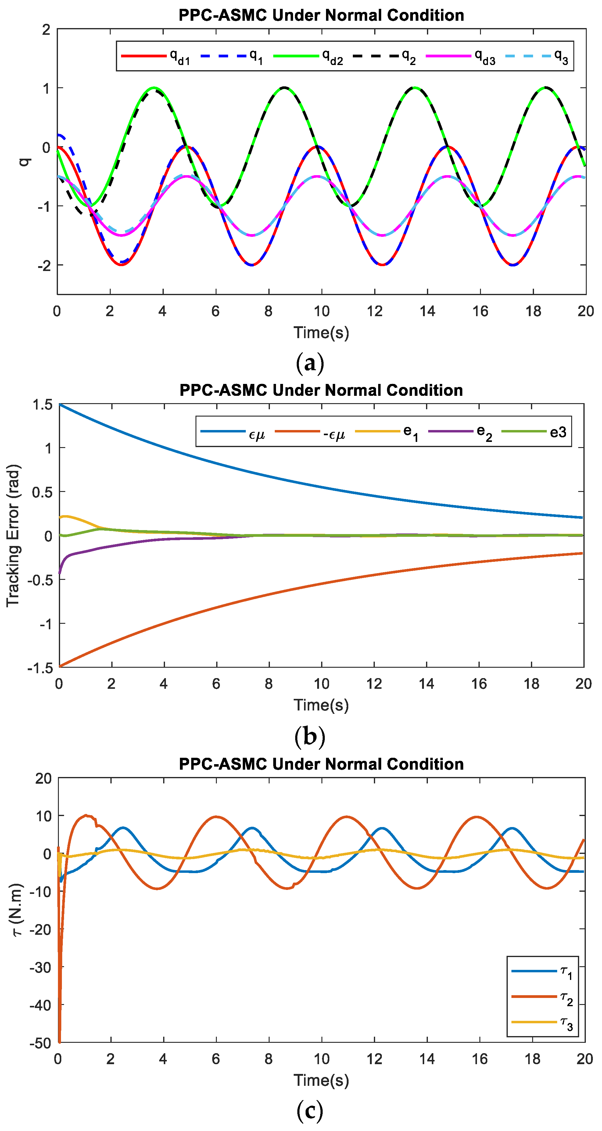
Now, the PPC-SMC controller is replaced with PPC-Adaptive Sliding mode control (PPC-ASMC) counterpart to further investigate the reference tracking of the manipulator system under the normal operating condition.
Figure 7,
Figure 8 and
Figure 9 indicate that this controller performs almost similar to the PPC-SMC controller in the normal condition and the tracking performance and the input torque quality are obtained properly.
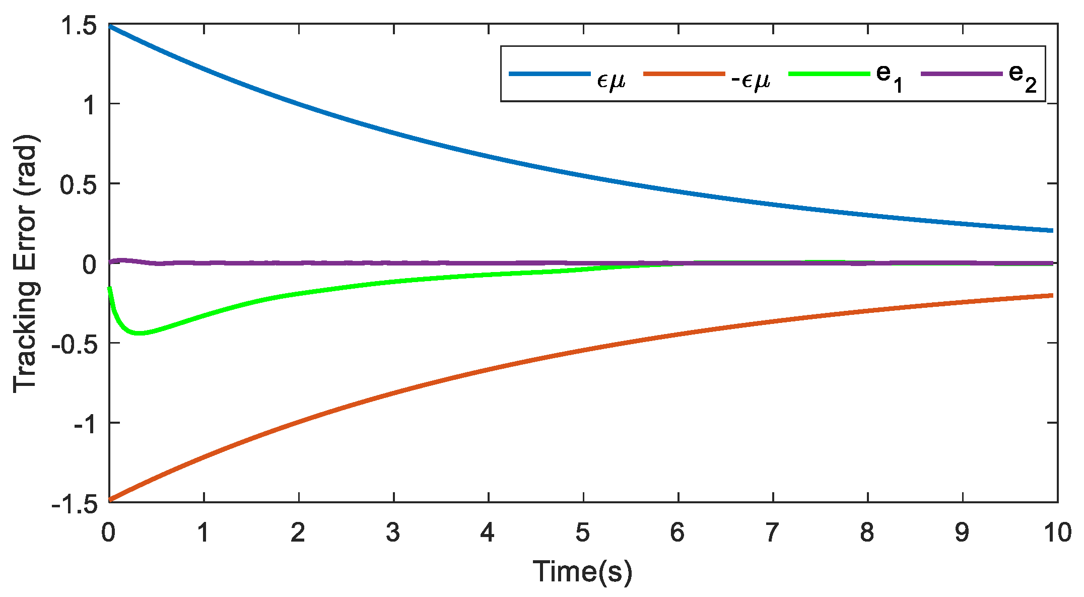
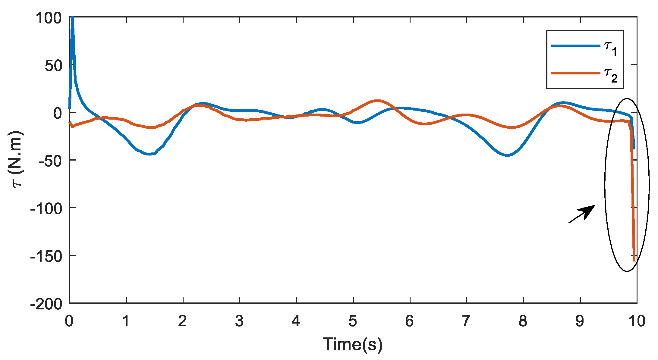
Scenario 2. Performance assessment under the uncertain condition
In this scenario, the PPC-SMC controller is utilized for the trajectory tracking of the manipulator system in the presence of model uncertainty. To this end, the nominal values of the parameters are changed by 20%, and an additive variable term as
is included into the system at
t = 5 s.
Figure 10,
Figure 11 and
Figure 12 demonstrate the results of this scenario. From
Figure 10 and
Figure 11, it is inferred that tracking errors, especially the second tracking error, is diverged from the stable condition at
t = 5 s, and this behavior is better observed at
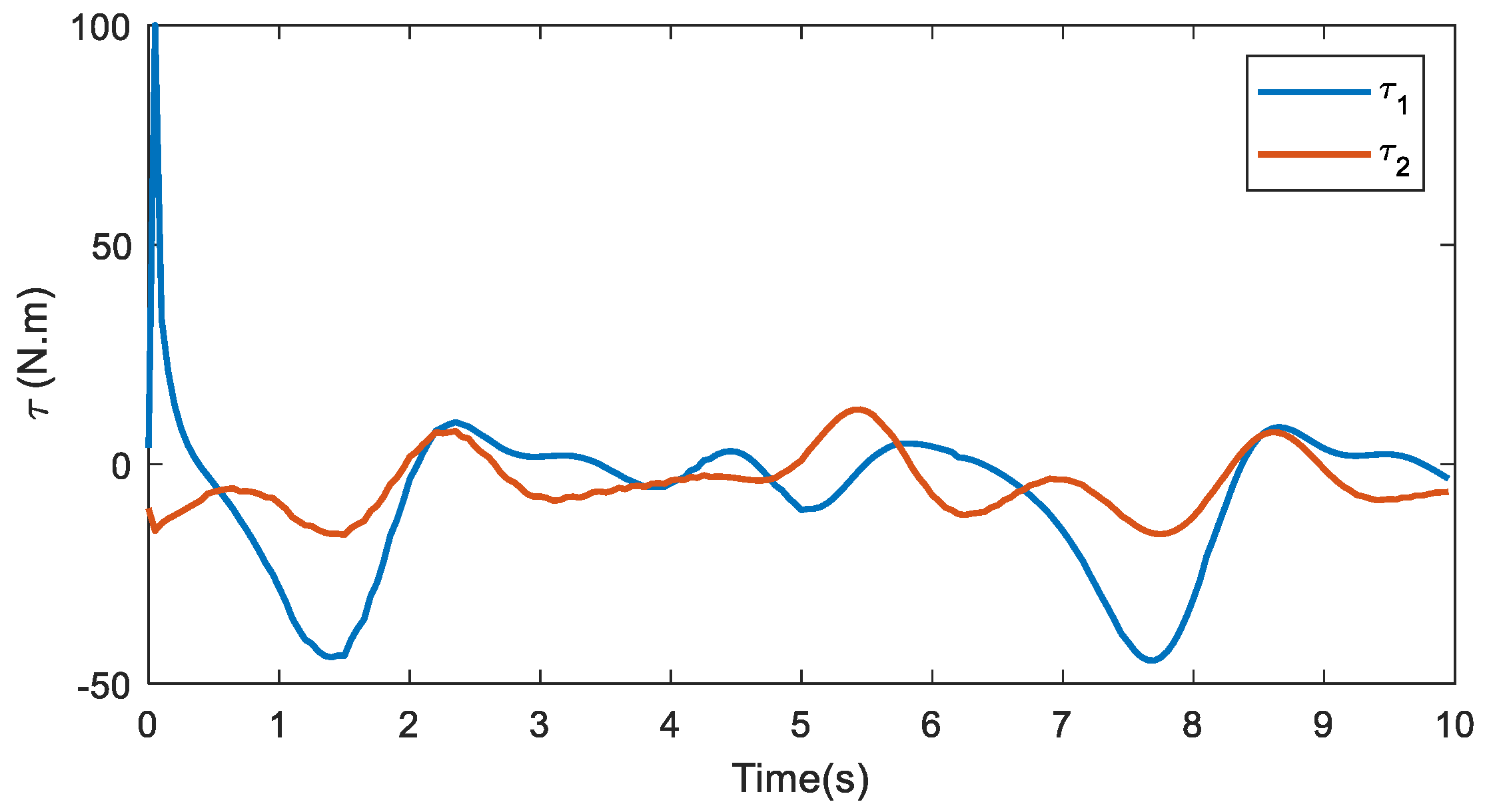
t = 8–10 s. The steady-state error increases in this condition. In
Figure 12, the input torque is noticeably disrupted at the final times of the simulation, by which the system cannot continue its normal operation. Moreover, this impact can result in physical damage to the system. Thus, the negative effects of uncertainties must be removed.
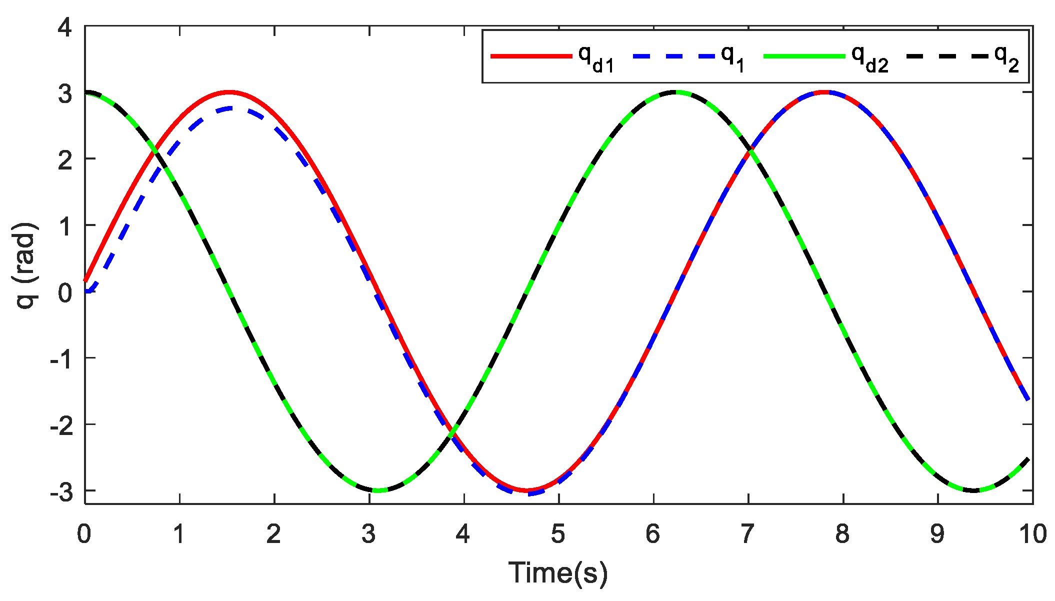
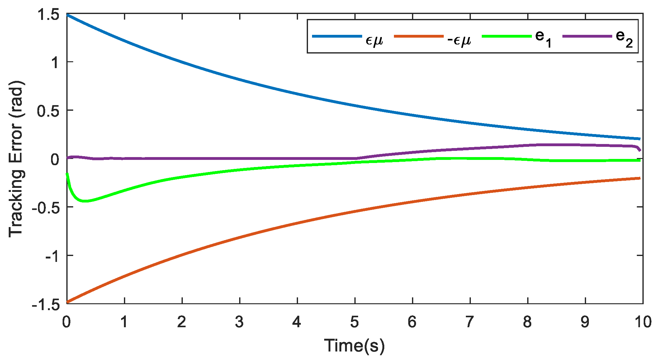
To compensate the effects of parameter uncertainties, the lumped uncertain term is estimated and eliminated through the online operation with the PPC-ASMC controller. The tracking and the input torque for each joint are illustrated in
Figure 13,
Figure 14 and
Figure 15. According to
Figure 13 and
Figure 14, the effect of uncertainties is well compensated, and the steady-state response is improved by adopting the ELM estimation. The input torques depicted in
Figure 15 are smooth enough and thus practically implementable. Consequently, the proposed controller is robust against model uncertainties regardless of the physical limits of the actuators. Moreover, tracking errors, as well as input torques, are obtained according to the PPC objective. Besides, the theoretical equations prove that this achievement is obtained within a finite time and the convergence rate criterion is satisfied. Inferred from
Figure 14, the tracking error is compensated in less than one second. To quantify the performance of the controller, the numerical performance metrics are used and the results are reported in
Table 1. In this table,
are performance indexes used to evaluate tracking precision based on
, and
is the performance index used to evaluate the input torque
.
Table 1 confirms that by applying PPC-SMC and PPC-ASMC to each joint of the manipulator in normal condition, acceptable tracking precision and input torque levels are achieved. However, this result is not maintained for PPC-SMC in the presence of uncertainties as all performance indices are changed towards a lower quality of operation, especially for the second joint of the robot. In
Figure 11, the decrease in tracking precision (evaluated by
and
) occurs from
t = 5 s. Moreover, by considering
Figure 12, it is inferred that the higher amount of
for PPC-SMC is directly related to the input torque recorded at the last times of the simulation, in which the controller is unable to compensate for uncertainties leading the system to reach the unstable condition. According to the numerical performance of PPC-ASMC in the uncertain condition, performance indices of the tracking precision and the input torque level are noticeably improved in comparison with PPC-SMC in the same operational condition. This fact reflects that ELM effectively improves the system performance in the presence of uncertainties. Thus, without extra control effort, PPC-ASMC reconstructs the robot’s performance.
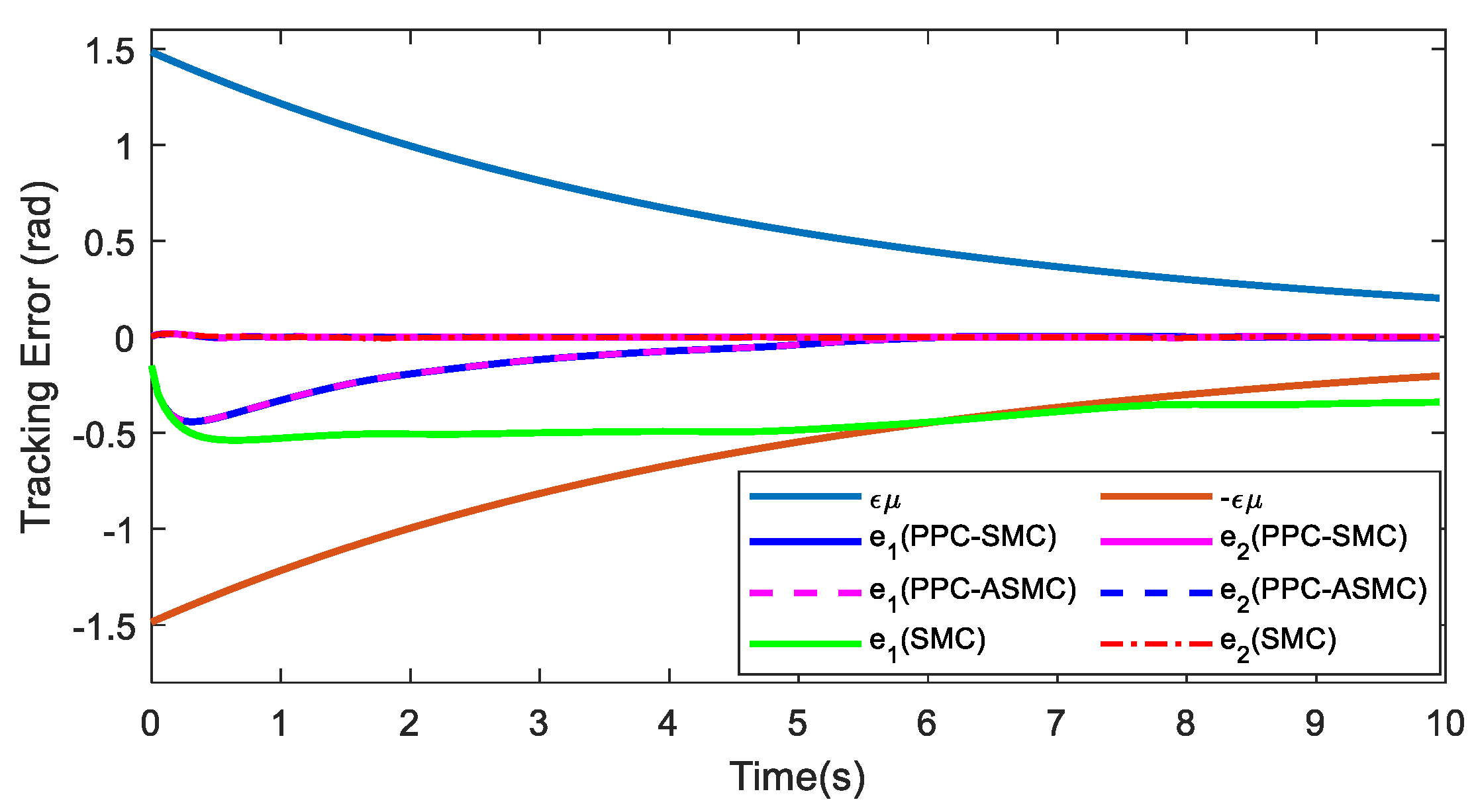
Scenario 3. Comparative study
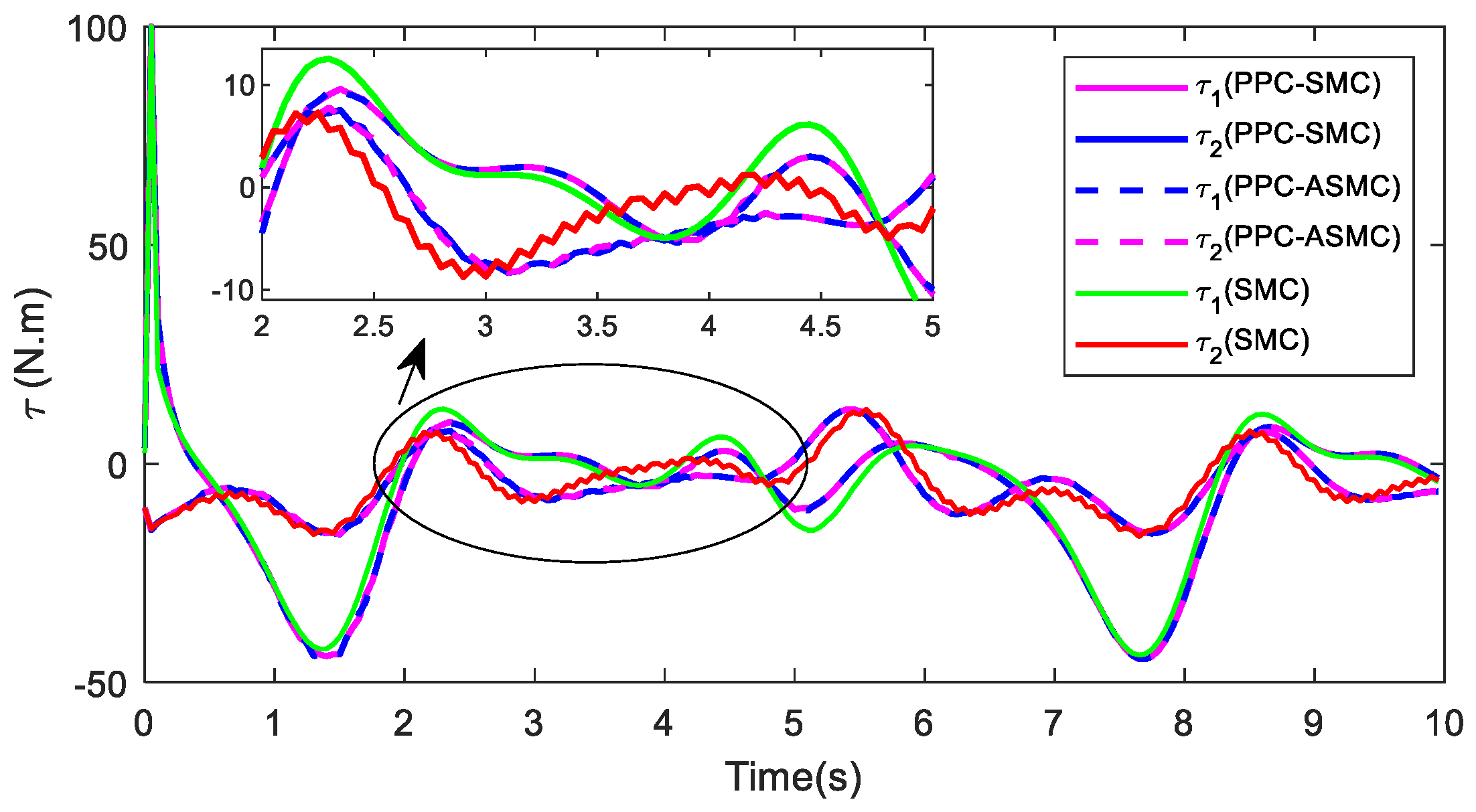
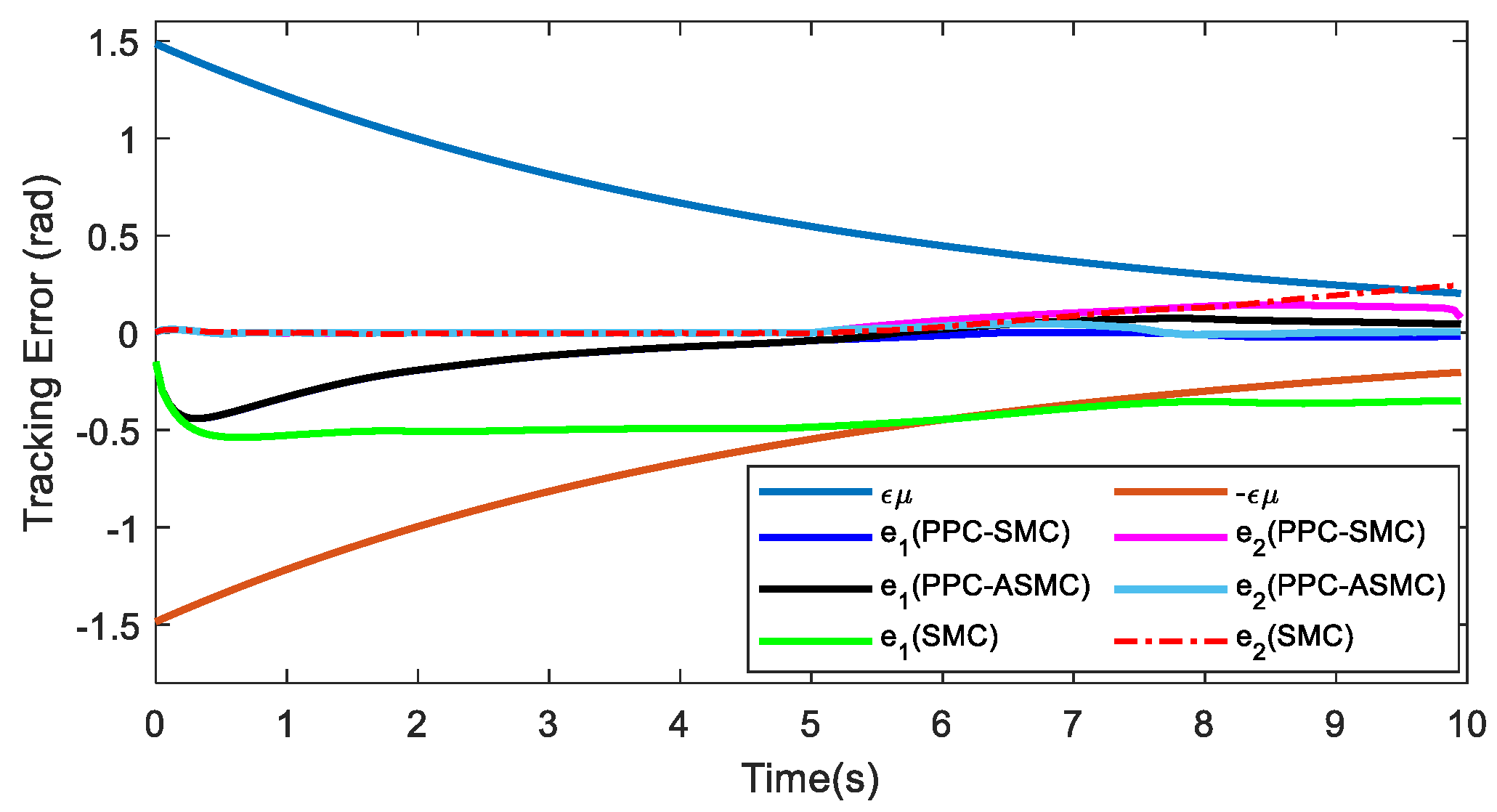
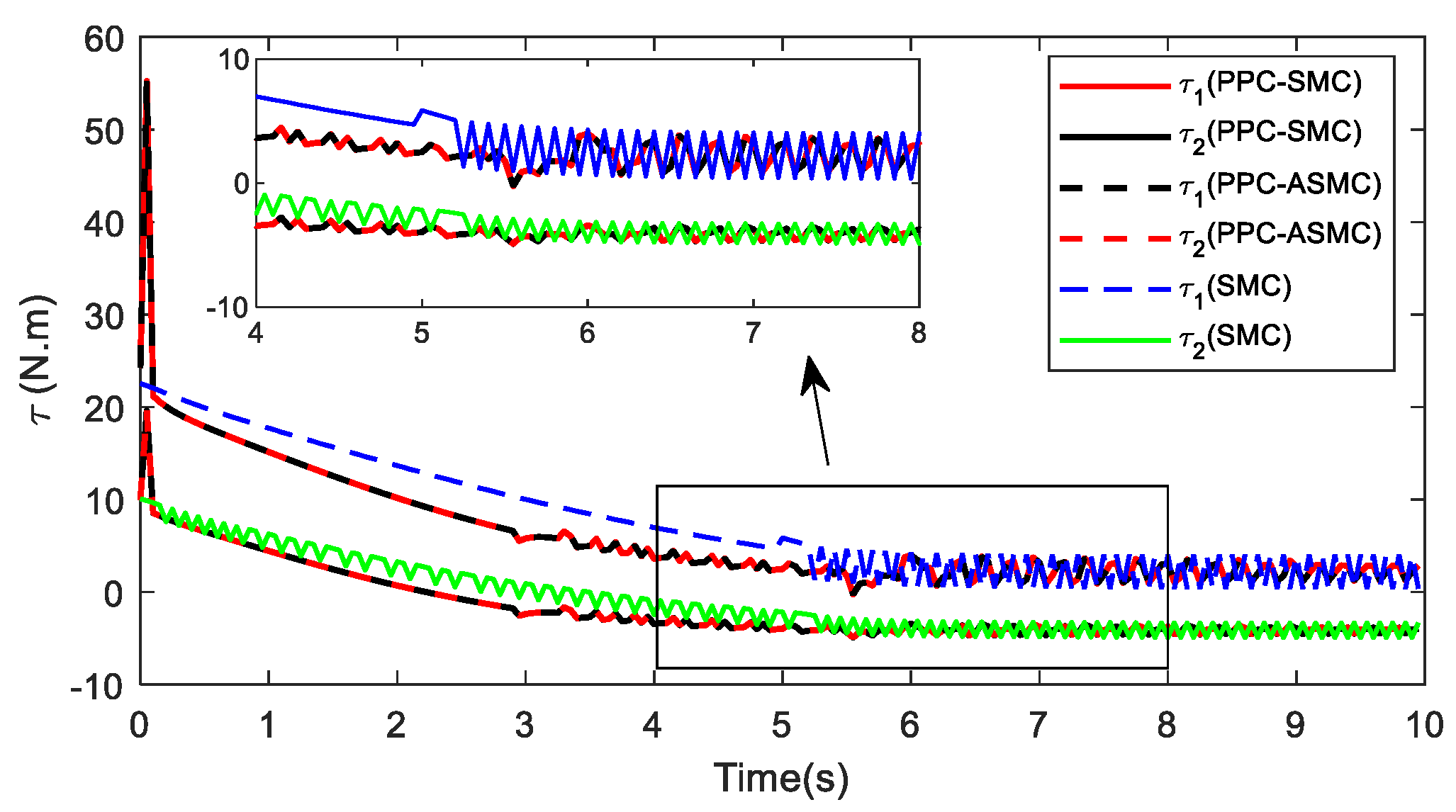
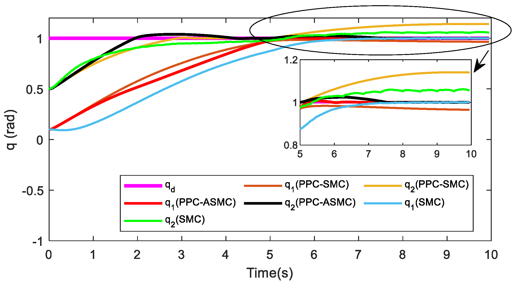
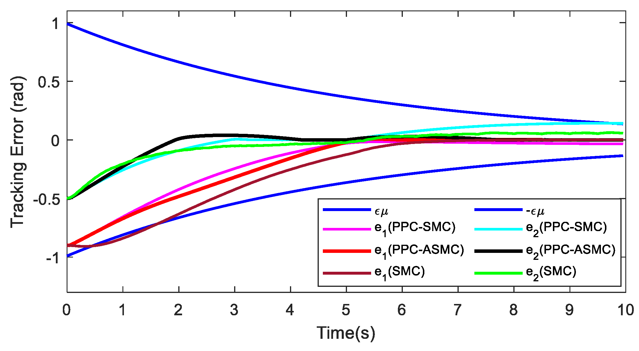
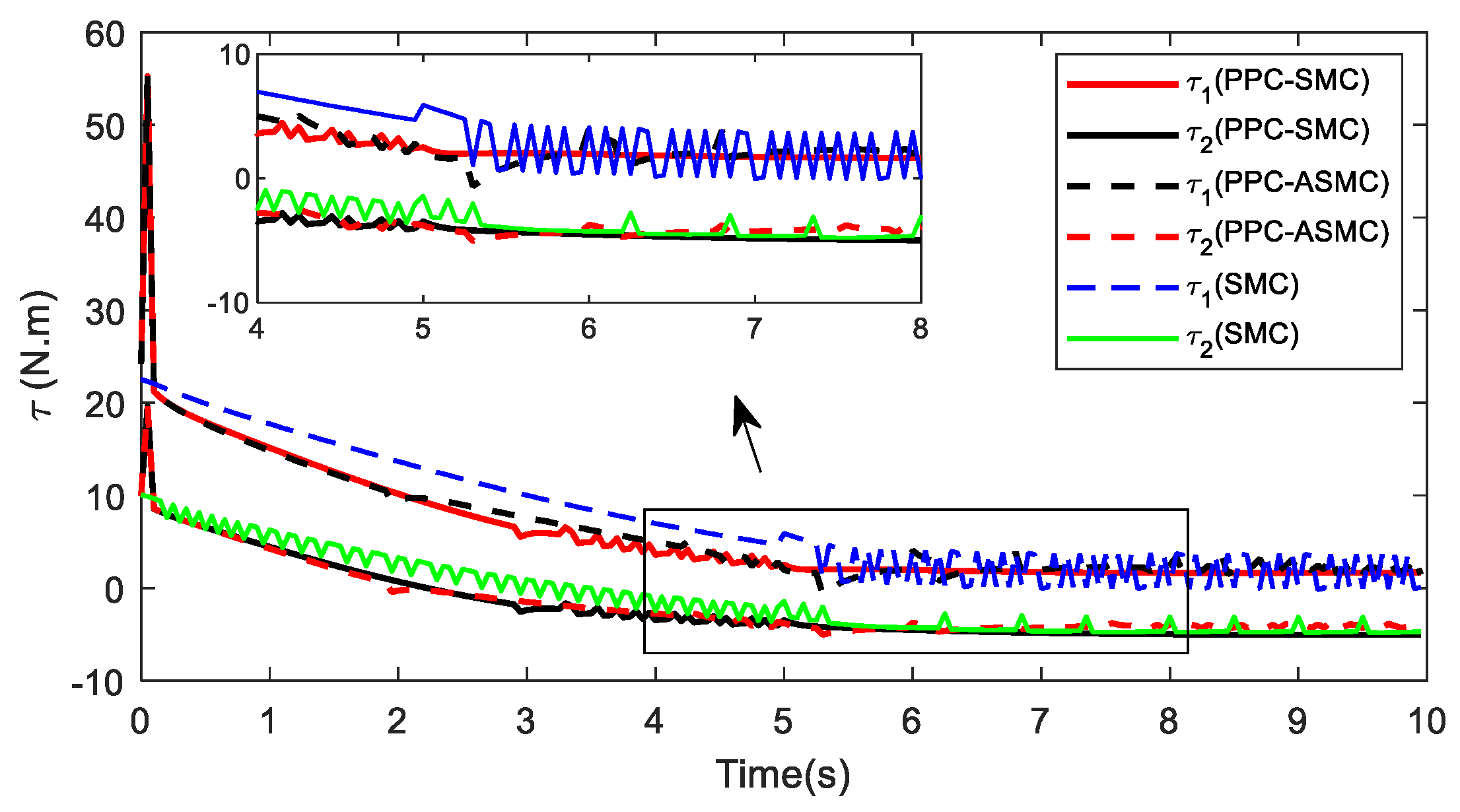
To further investigate the effectiveness of the controller, PPC-SMC and PPC-ASMC controllers are compared with the conventional SMC by analyzing tracking errors and input torques of both controllers in the normal condition.
Figure 16 and
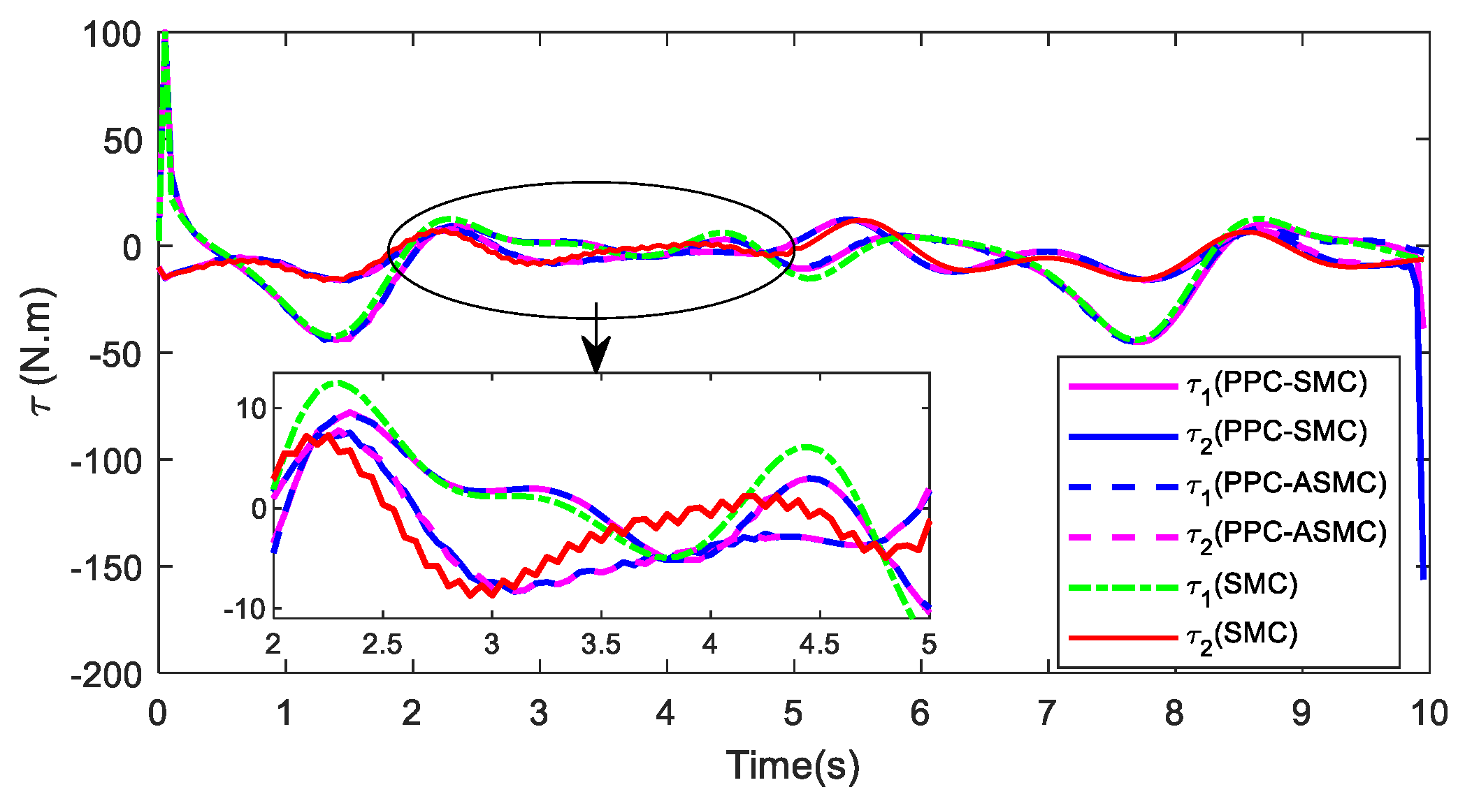
Figure 17 shows the results of simulation for this scenario. These figures indicate that the conventional SMC is not as accurate as the proposed PPC-ASMC controller because the respective tracking error of the first joint (indicated by the green color) is outside the prescribed region. Furthermore, the quality of the input torque, depicted in
Figure 18, is better for the proposed controller. While the input torque of the conventional SMC, especially the second SMC input torque (indicated by the red color), is obtained with chattering effects. Consequently, it is perceived that there is no regulation between the input torques and the tracking errors of SMC. If the error tracking is desirable, the respective input torque degrades with chattering signals. Similarly, a high-standard input torque cannot drive the robot end-effector towards the desired reference with enough precision.
Next, the performance comparison is investigated in the uncertain condition for PPC-SMC, PPC-ASMC, and SMC controllers.
Figure 19,
Figure 20 and
Figure 21 summarize the results for this scenario. From
Figure 19 and
Figure 20, it is observed that the PPC-ASMC controller is able to compensate for uncertainties, and the steady-state error of each joint reaches zero with enough accuracy as confirmed in Scenario 2. It should be mentioned that since the ELM approximation is performed with random inputs, there is some discrepancy between each pair of estimations and results. As shown in
Figure 19 and
Figure 20, the conventional SMC is not effective in dealing with uncertainties, and the tracking error diverges from the stable condition in the steady-state case. Thus, this method is not proposed in any condition since the uncertain term is indispensable in real applications, and this controller is prone to result in failures. Although a compromise between precision and the input torque quality could be fairly obtained by proper selections of the SMC gains, this adjustment would be costly, time-consuming, and not reliable. Similarly, the PPC-SMC controller does not provide acceptable results since it eventually becomes unstable in the uncertain condition. Consequently, among the three controllers, only PPC-ASMC provides the desired results in the uncertain condition.
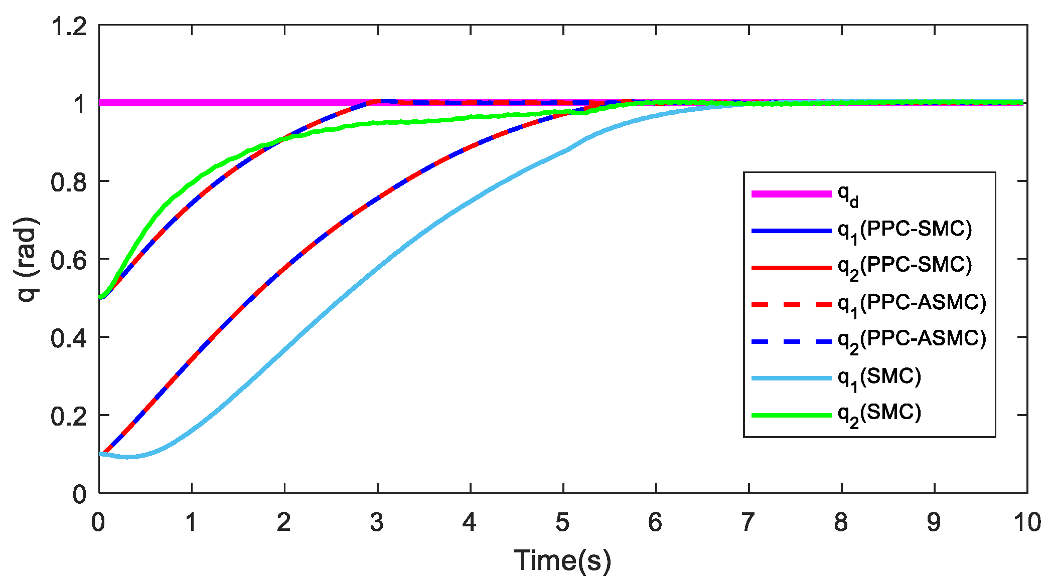
To further elaborate the comparative study, the transient performance of the controllers in both normal and uncertain conditions is investigated with respect to the step response. In this scenario, the prescribed function is set as
. The SMC parameters are selected as
,
. The initial state for each joint is set as
Figure 22,
Figure 23 and
Figure 24 show the results of this scenario. According to
Figure 22 and
Figure 23, both PPC-SMC and PPC-ASMC performs well in normal condition. The respective tracking errors are within the prescribed region, reaching the desired position before
t = 6 s. Furthermore, the input torques for PPC-SMC and PPC-ASMC are obtained considerably smoother than SMC, however, with a higher initial value. The step response of SMC is not desirable as the output error of the first actuator (depicted by the blue color) is not inside the prescribed region in the initial operation. Furthermore, the convergence rate of this response is considerably slow. This is in addition to the undesirable SMC input torques with chattering effects, which are highly destructive. Thus, SMC cannot perform well in normal condition, while the counterparts satisfy the control objectives in this condition.
Finally, the step responses of the mentioned controllers are compared with each other under the uncertain condition. In this case, the nominal values of the parameters are changed by 20%, and an additive variable term as
is inserted into the system at =5 s. The results are illustrated in
Figure 25,
Figure 26 and
Figure 27.
Figure 25 and
Figure 26 confirm the superiority of the PPC-ASMC controller over the PPC-SMC and SMC controllers. Adding the uncertain term into the system, the PPC-ASMC controller ensures accuracy with smoother torques, similarly to the normal condition. Considering the PPC-SMC controller, although the step response for the first joint can meet the desired response, the step response of the second joint diverges from the stable steady-state mode. This highlights the fact that regardless of the initial high amplitude, this controller is not reliable in uncertain conditions. Regarding the SMC step response in the uncertain condition, not only the transient response is not desirable, but also the steady-stated response is not achieved. Inferred from
Figure 25 and
Figure 26, the first robot joint is not located in the desired region in the transient mode. Moreover, the second robot joint diverges from the steady-state point. This is in addition to the undesired SMC inputs, which are obtained with considerable chattering effects, which are clearly seen in
Figure 27. Consequently, the proposed PPC-ASMC controller satisfies both the transient and steady-states desired responses under both normal and uncertain conditions. This result is aligned with a fast convergence rate, which is achievable and regulatable by a designer.
The last section of the simulation works is dedicated to investigating the effectiveness of the proposed controller on PUMA 560, which has been widely used in different research and practical applications. The details of its model are given in [
33], and for the sake of simplicity, only the three joints of this robot are analyzed in simulations. In this regard, the proposed PPC-ASMC controller is compared with PPC-SMC, SMC, and the Fuzzy-PID controller for PUMA 560. The reference signal is given to the manipulator’s joints as
. Regarding PPC-SMC and PPC-ASMC,
The PID-based SMC (PID-SMC) controller designed in [
34] is used in the following comparisons. The input torque of this method is as
, computed by using the sliding surface
,
is a small positive constant and
is a known constant for the upper bound of uncertainties (
). The Fuzzy-PID controller is adopted according to the method presented in [
35]. The simulation results of the normal conditions are illustrated in
Figure 28,
Figure 29,
Figure 30 and
Figure 31.
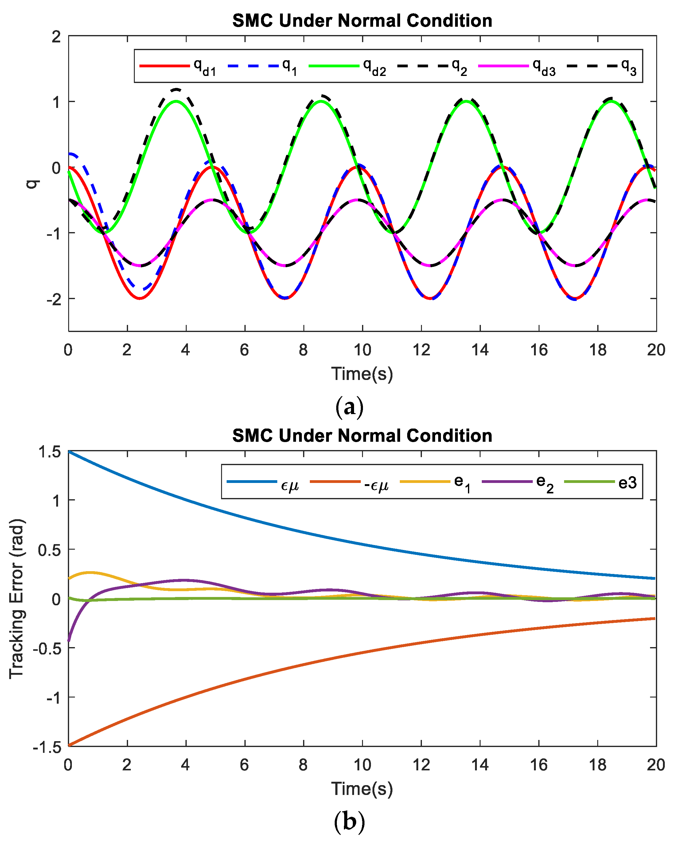
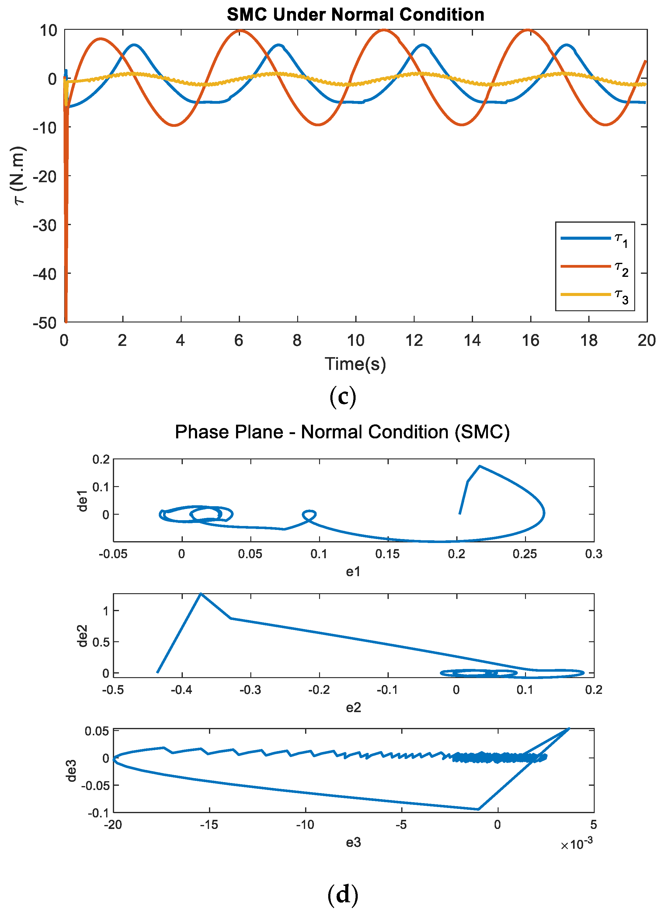
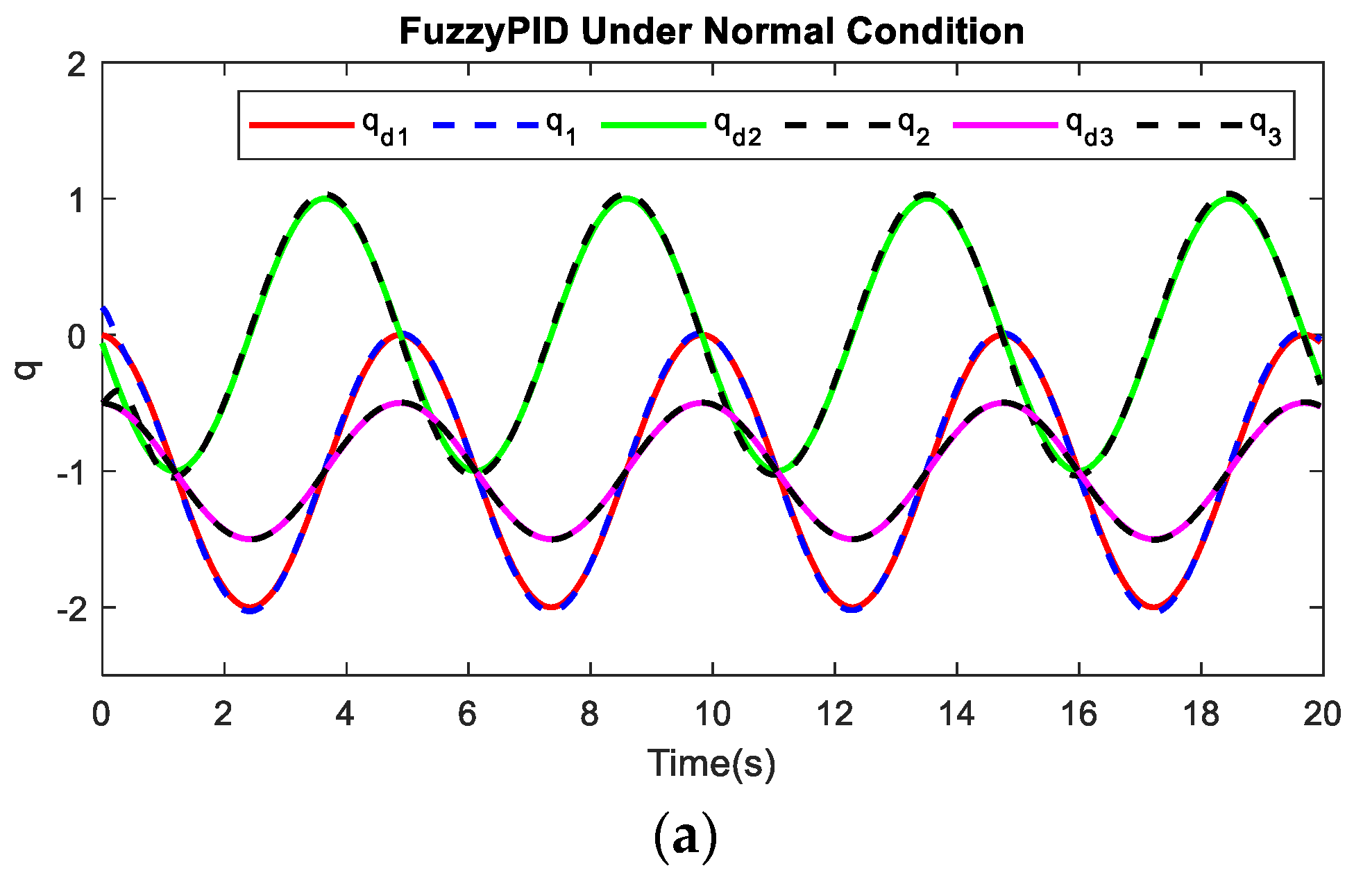
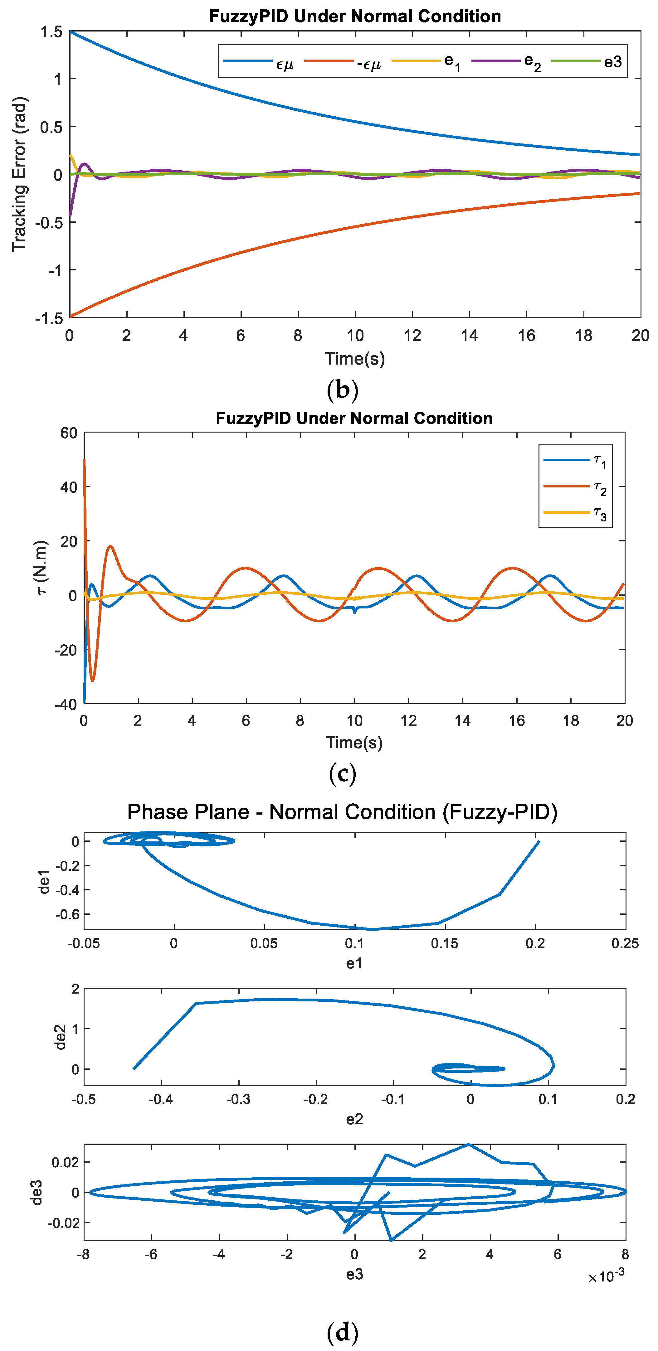
Figure 28,
Figure 29,
Figure 30 and
Figure 31 show that all the controllers perform well in normal condition. Both PPC-SMC and PPC-ASMC have similar responses in terms of precision and input torque features. The parameters of the SMC are tuned to provide a trade-off between accuracy and the chattering effects. Thus, although it does not have high accuracy, it performs with negligible chattering effects. Regarding the Fuzzy-PID controller, the tracking response of this method is obtained with desirable precision and input torque quality. The numeric evaluation of the controllers in normal condition is presented in
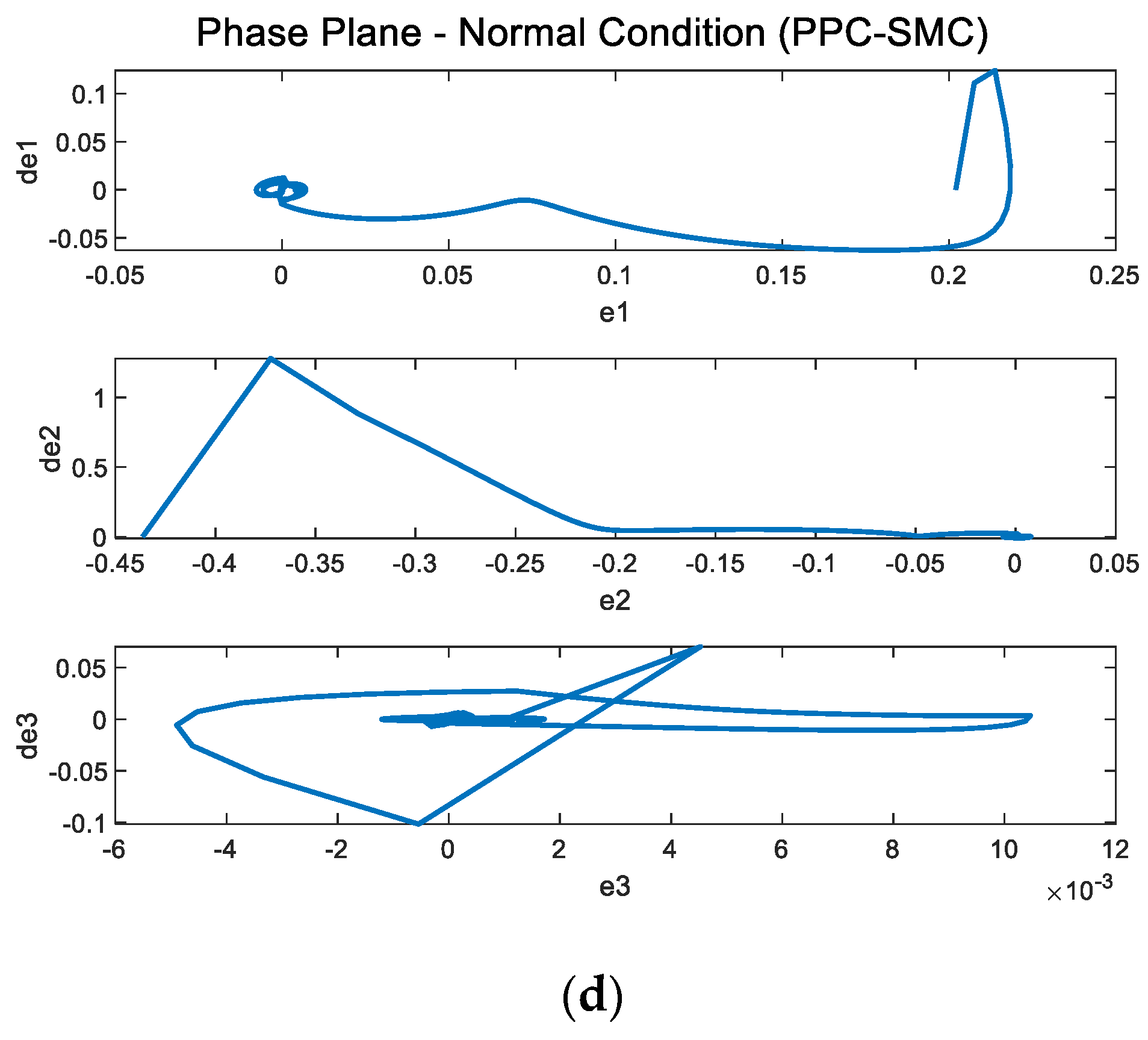
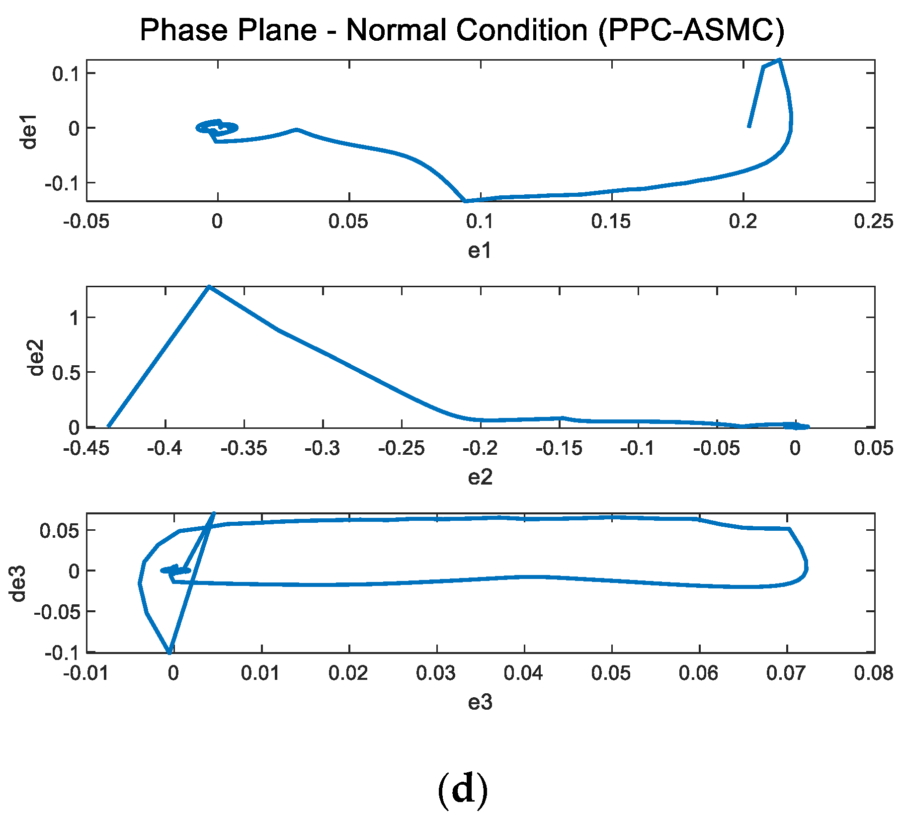
Table 1. Since the response speed of the controller is important for practical applications, this performance index is used in evaluations along with the precision and control effort criteria. The performance of each controller is analyzed by drawing the phase plane of the tracking errors. Regarding the figures indicated by (d) in normal conditions, it can be seen that all controllers result in a stable steady-state response as all the tracking errors reach zero within a finite time.
According to
Table 1, SMC requires the least amount of time (0.6 s) to fulfill its task in normal condition. The speed comparison is followed by PPC-ASMC and PPC-SMC, which require a moderate amount of time (1.4 s) to complete their tasks. By far, Fuzzy-PID controller requires considerable long time to finish the tracking performance.
Now, the overall control performances can be better evaluated in normal condition. All the mentioned controllers require almost the same control effort. Although Fuzzy-PID controller provides high accuracy, this method is not suitable for practice considering the computational expenses. The SMC provides the best performance in terms of accuracy and speed response in this condition. Both PPC-SMC and PPC-ASMC are in the second-best place in normal condition.
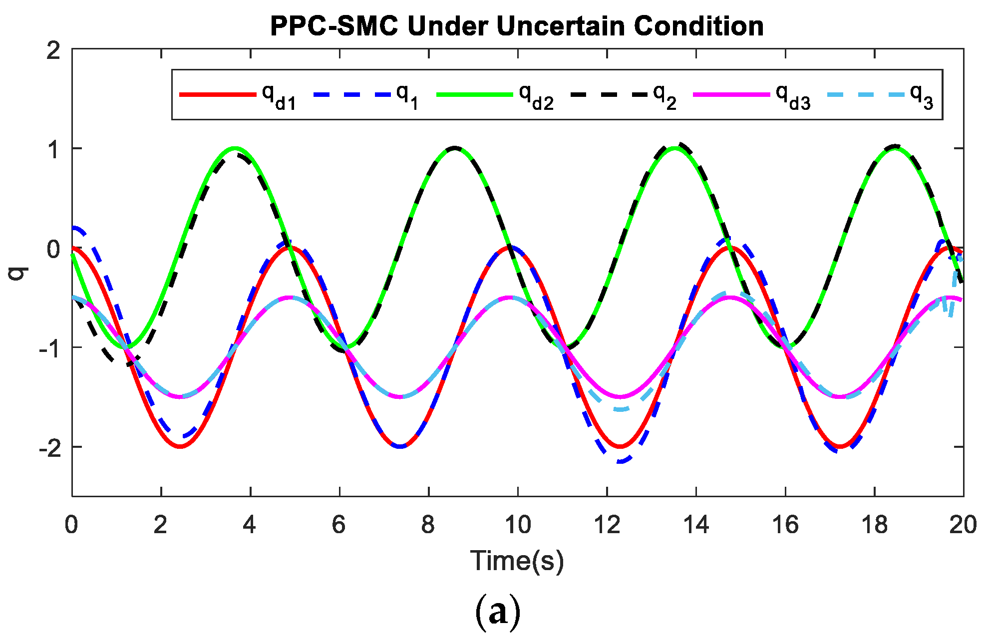
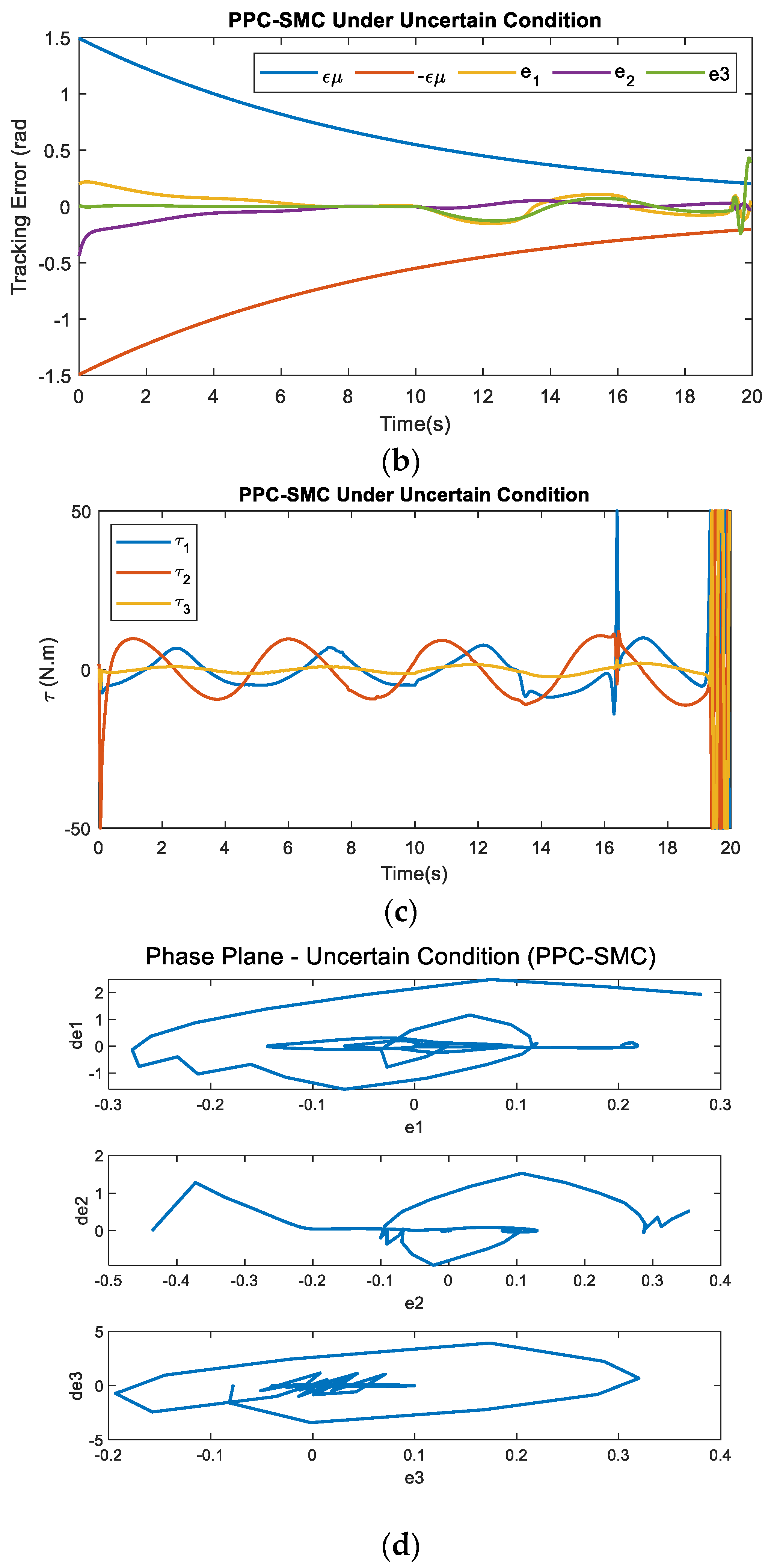
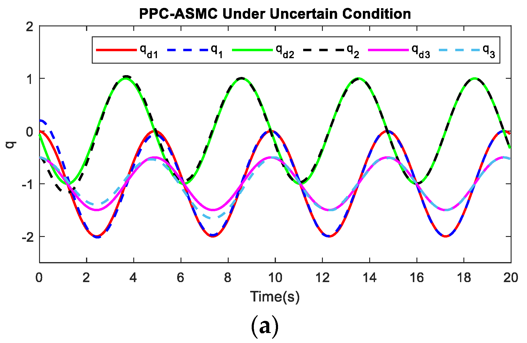
Next, the previous comparison is repeated for PUMA 560 in uncertain condition. The lumped uncertainty is added to the system at
t = 10 s as
and the inertia matrix of the system is increased by 40% (1.4 M, for example, payload changes at this time).
Figure 32,
Figure 33,
Figure 34 and
Figure 35 and
Table 2 provide detailed performance evaluation of the mentioned approaches qualitatively and numerically, respectively.
The performance assessment of the system in the uncertain operating condition is reported in
Table 3.
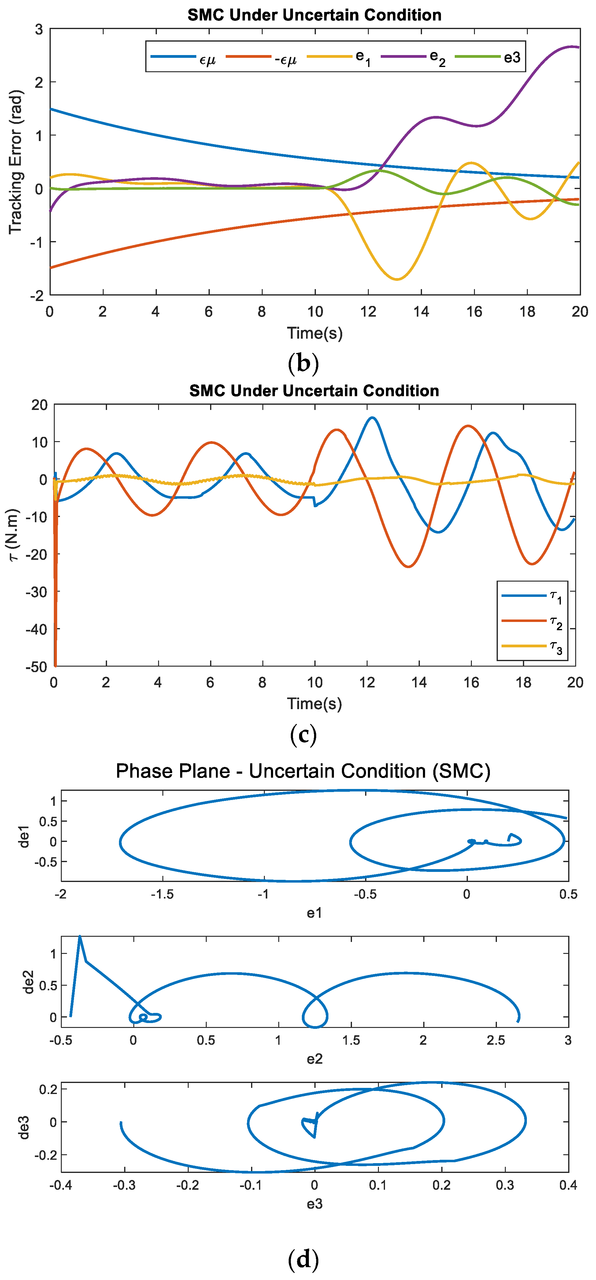
According to the results, although SMC offers the best results in normal conditions, it cannot lead to the same result in uncertain conditions. As illustrated in
Figure 34, reference tracking is disrupted after the insertion of uncertainties, and the tracking errors violate the predetermined boundary. From
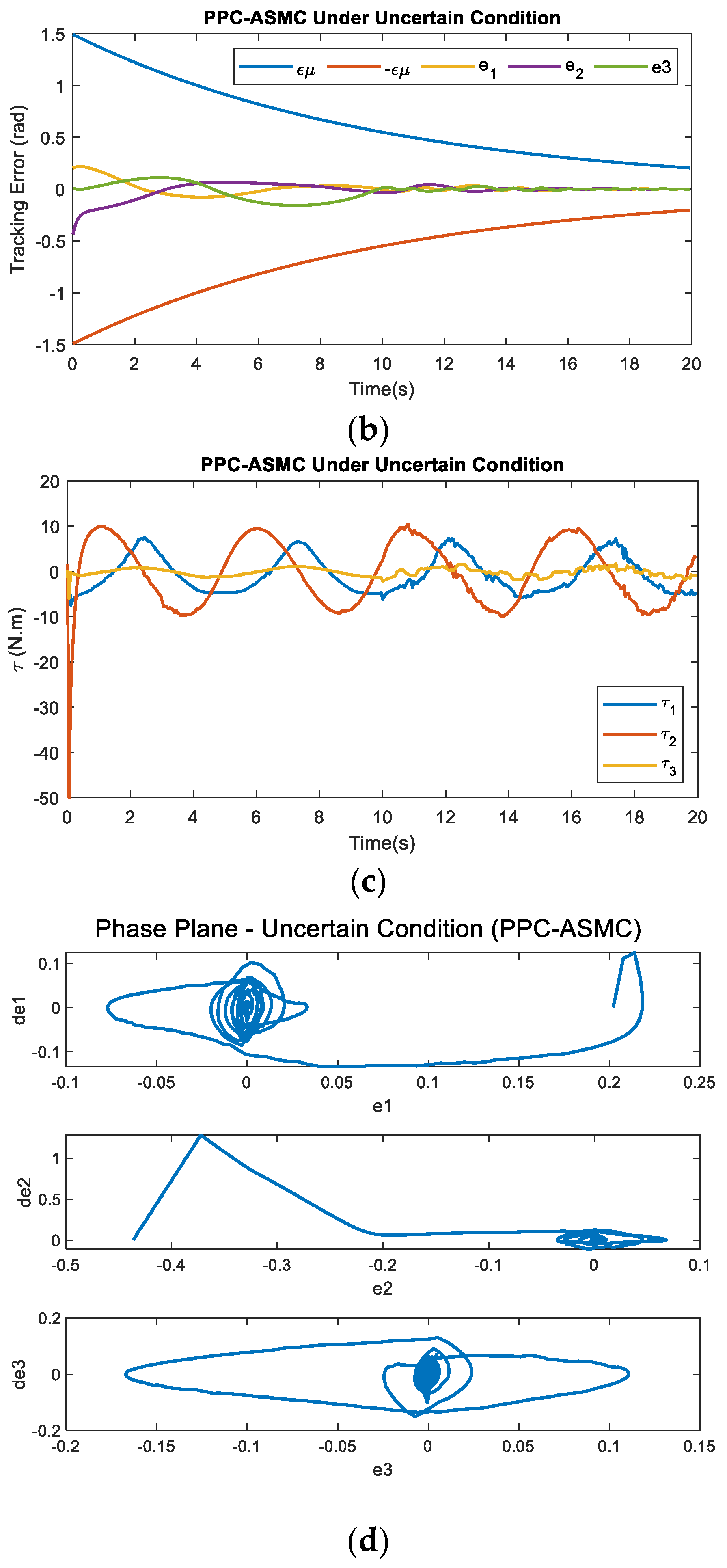
Figure 35, well tracking of the Fuzzy-PID controller in the uncertain condition is observed. However, this performance is overshadowed by the computational complexity of this method. Regarding both qualitative and numerical assessment, the quality of PPC-SMC decreases as uncertain terms are applied, and even with adopting more control efforts it is not able to compensate the uncertain effects. Interestingly, PPC-ASMC keeps its well-tracking performance even when uncertainties are inserted continuously from
t = 10 s.
Figure 33 represents the ability of PPC-ASMC in the presence of uncertainties without requiring more control effort. Although this result is obtained with minor chattering effects, all other criteria, including control effort, performance speed, precision, and robustness, are desired for this controller. Following the analysis, the phase plane of each tracking error is given. Regarding the phase plane of PPC-ASMC, it is clear that this controller leads to steady-state stability in uncertain conditions. However, the phase plane for PPC-SMC and SMC in uncertain conditions are not as desired as their respective phase plane in normal conditions. The phase plane of Fuzzy-PID in uncertain conditions is the same as its phase plane in normal conditions. Consequently, PPC-ASMC provides the best overall performance among all the investigated methods.


