
VLP Landmark and SLAM-Assisted Automatic Map Calibration for Robot Navigation with Semantic Information


1
HKUST Shenzhen-Hong Kong Collaborative Innovation Research Institute, Shenzhen 518055, China
2
The State Key Laboratory of Advanced Displays and Optoelectronics Technologies, ECE Department, The Hong Kong University of Science and Technology, Hong Kong SAR, China
*
Author to whom correspondence should be addressed.
Robotics 2022, 11(4), 84; https://doi.org/10.3390/robotics11040084
Submission received: 24 July 2022
/
Revised: 19 August 2022
/
Accepted: 19 August 2022
/
Published: 21 August 2022
(This article belongs to the Topic Intelligent Systems and Robotics)
Abstract
:With the rapid development of robotics and in-depth research of automatic navigation technology, mobile robots have been applied in a variety of fields. Map construction is one of the core research focuses of mobile robot development. In this paper, we propose an autonomous map calibration method using visible light positioning (VLP) landmarks and Simultaneous Localization and Mapping (SLAM). A layout map of the environment to be perceived is calibrated by a robot tracking at least two landmarks mounted in the venue. At the same time, the robot’s position on the occupancy grid map generated by SLAM is recorded. The two sequences of positions are synchronized by their time stamps and the occupancy grid map is saved as a sensor map. A map transformation method is then performed to align the orientation of the two maps and to calibrate the scale of the layout map to agree with that of the sensor map. After the calibration, the semantic information on the layout map remains and the accuracy is improved. Experiments are performed in the robot operating system (ROS) to verify the proposed map calibration method. We evaluate the performance on two layout maps: one with high accuracy and the other with rough accuracy of the structures and scale. The results show that the navigation accuracy is improved by 24.6 cm on the high-accuracy map and 22.6 cm on the rough-accuracy map, respectively.
1. Introduction
With the development of sensors, control systems, bionics and artificial intelligence, robot technology has been investigated and applied in many areas to provide services such as hospital inspection, hotel delivery and warehouse logistics. Using mobile robots in indoor environments can effectively improve the intelligence and effectiveness of task execution. By combining robot intelligence and human expertise, human–robot interaction is promoted in multiple scenarios, such as medical applications [1,2] and industrial applications [3,4]. Meanwhile, in these robot applications, navigation plays an increasingly crucial role. As an essential element in the navigation process, high-precision positioning in indoor environments is still a challenging task. Since the Global Navigation Satellite System (GNSS) cannot provide satisfactory positioning services in indoor environments due to the extreme signal attenuation and interruption caused by indoor structures, WiFi/Bluetooth fingerprinting-based indoor positioning systems (IPSs) have raised extensive attention and achieved encouraging results. However, positioning based on WiFi/Bluetooth can only achieve meter-level accuracy [5].
Compared with WiFi/Bluetooth fingerprinting-based positioning, positioning with landmarks composed of visible light positioning (VLP)-enabled lights can provide an absolute location when using an image sensor as a receiver. Scanning of the whole area is not required, and global 3D positioning results can be achieved as long as the 3D position information of the landmarks is encoded in the VLP lights. In our previous works [6,7], we proposed a VLP system based on a single LED that could achieve centimeter-level accuracy, with an average accuracy of 2.1 cm for a stationary robot [6] and of 3.9 cm for a 3D tilted receiver camera [7].
Besides positioning, building an accurate map is another important element for navigation because both positioning and path planning rely on the map information of the environment [8]. One typical map representation is an occupancy grid map [9], in which the value of each cell represents the probability of being occupied by obstacles. Currently, Simultaneous Localization and Mapping (SLAM) technology [10] is widely used to determine the position of the robot and build an occupancy grid map at the same time by fusing available sensor information. However, SLAM has three main drawbacks. The first is that SLAM can only determine a local position and the relative movement of the robot in the environment [11]. Second, SLAM requires scanning and survey of the whole scene to obtain a map. Last, the position based on the sensors in the robot, including the odometer and inertial measurement unit (IMU) will drift and lose global accuracy with time [12]. These drawbacks lead to challenges for mapping and navigation in large-scale and multi-floor environments.
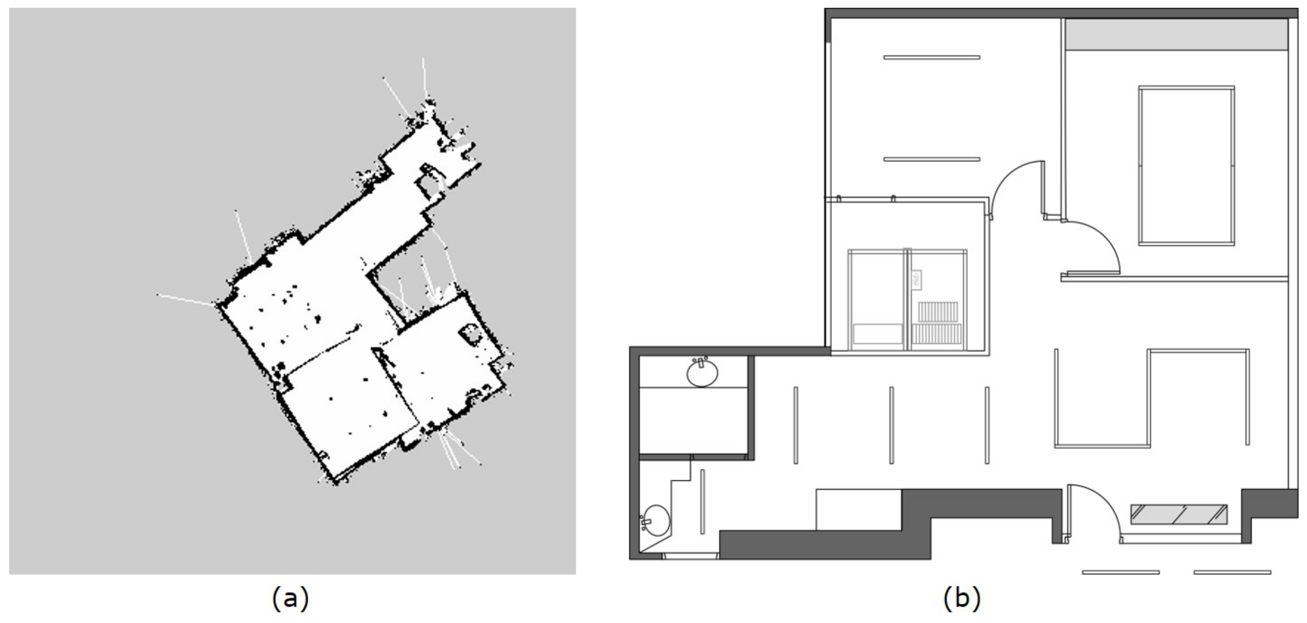
In addition, the occupancy grid map created by SLAM only contains three types of information: the cell is occupied, free of obstacles or unknown to the robot, as shown in Figure 1a. There is no semantic information on the structures. Moreover, the occupancy grid map may not be oriented so that humans can distinguish the direction with a correspondence to the real world. The noise from the sensors will also be shown on the map and mislead the robot as well as humans. Therefore, it is noticeably difficult for humans to understand an occupancy grid map generated by a robot and send commands to the robot based on it.
Noting the drawbacks of the occupancy grid map generated by SLAM and its difficulties for humans, we propose to use a layout map to promote better cooperation between humans and robots. A human in an indoor environment will always use a layout map, which illustrates structures and contains semantic information, to navigate a pathway from the current position to the target position, as shown in Figure 1b. A layout map always demonstrates the whole area and is complete and without noise. The boundaries on such maps refer to obstacles in the area that cannot be crossed by a robot and have the same meaning as the occupied cells in an occupancy grid map. However, the accuracy of a layout map in terms of resolution cannot be guaranteed, which will degrade the accuracy and reliability of navigation.
Therefore, in this paper, we propose to calibrate the layout map of a scene using the occupancy grid map generated by SLAM to improve navigation performance. In the mapping process, an image sensor is mounted on the robot and we use VLP landmarks to acquire the robot’s position on the layout map. At the same time, SLAM is performed on the robot, and its position on the occupancy grid map is determined by the sensors. After at least two landmarks are tracked by the image sensor on the robot, the occupancy grid map generated by SLAM is saved as a sensor map. Then, the orientations of the two maps are aligned based on the pixel coordinates of the tracked landmarks on the maps. Moreover, the scale of the layout map is calibrated by computing the pixel distance between the key points. To keep the consistency of the map image after scaling, the eight-neighborhood averaging method and bi-linear interpolation method are applied. It is noteworthy that the map calibration method based on landmarks is scalable to scenes mounted with multiple landmarks by computing the average of the rotation angle and scale of every two key points. Finally, to verify the effectiveness of the proposed map alignment methods, we develop the algorithm on the robot operating system (ROS) and perform real-time experiments. In the mapping experiment, we calibrate the layout map with different numbers of VLP landmarks to evaluate the map alignment performance. We further perform robot autonomous navigation on the calibrated map to evaluate the navigation results after map calibration. A navigation experiment with semantic information is also performed to visualize how semantic information can help humans to send instructions to robots.
More explicitly, the main contributions of this paper include: 1. VLP is utilized as a landmark to achieve robot positioning on the layout map; 2. homogeneous transform matrices are applied to align the layout map with SLAM produced occupancy grid map; 3. the proposed map calibration method is evaluated by robot autonomous navigation with semantic information.
The paper is organized as follows. Related work is introduced in Section 2. Section 3 explains the mapping system and map transformation process. In Section 4, we present the details of the proposed VLP landmarks and SLAM-assisted automatic map calibration method. Experimental results are provided and analyzed in Section 5. Finally, Section 6 concludes this paper.
2. Related Work
2.1. Robot Positioning and Navigation
Robot autonomous navigation is a crucial component when developing robot intelligence in various scenarios, such as transportation, medical science and agriculture. The application of a transport robot aims to improve work efficiency by saving human labor resources and meanwhile guarantee strong safety in industrial automation and production [13]. An operational strategy for the task allocation and path planning of multiple transport robots is proposed in [14], which can minimize the task time. In the medical industry [15], a navigation robot can also minimize person-to-person contact, taking an essential role in the clinical management during the COVID-19 pandemic [16]. A complete pipeline of robotic assistance in drug delivery is proposed in [17], using the navigation robot to realize efficient interaction with patients and doctors and monitor drug intake. Robot autonomous navigation is a challenge in agriculture caused by the semi-structured environment and uneven ground [18]. To achieve safe navigation on a steep slope, a path planning method aware of the robot’s center of mess is proposed in [19], taking into account the specific limitations of the environment including the limited steering angles and a preference for forward motion.
When achieving robot autonomous navigation, positioning technology plays an essential role. In a robot positioning system, there are two types of sensors [20]. One is onboard sensors, which adhere to the robot body, such as the odometer and IMU. These sensors measure the robot’s linear and angular velocities and accelerations with a high updating rate, and predict its position and orientation by previous measurement. An indoor positioning system based on wheel odometry is proposed in [21] by fusing the readings from an encoder, gyroscope, and magnetometer using a self-tuning Kalman filter coupled with a gross error recognizer. In [22], two IMUs are used to estimate the position, and the positioning performance is improved by the implementation of the relative relationship. The average positioning accuracy is lower than 20 cm over short periods of time. However, since the onboard sensors are subject to time-dependant integral error that increases over time [23], the accumulated error is still inescapable, leading to the degradation of positioning accuracy.
The other type is external sensors, which are separated from the robot body, such as image sensors and light detection and ranging (LiDAR). These sensors are capable of measuring an absolute position with the aid of a fixed global reference in the environment. In [24], a radio-frequency identification (RFID) reader is mounted on the robot to track its position in the scene where RFID tags are placed at each intersection of structured environment ways. A Bayesian filter-based robot positioning system with RFID tag collecting is proposed in [25], and the average positioning accuracy is about 50 cm. In [26], the robot is equipped with an array of microphone, and the positioning is achieved using the time difference of arrival (TDOA). An unscented Kalman filter-based position estimation method is proposed in [27], where a tachometer is mounted on the robot. To increase the positioning accuracy, more sensors, such as IMUs, are needed. In [28], a bio-mimetic radar sensor-based positioning system is proposed, and it can locate a robot with an average accuracy of 35 cm. A moving camera localization method is proposed for scenes with repetitive patterns by adaptively selecting distinctive features or feature combinations [29]. Compared with these works, VLP can achieve much better, centimeter-level, positioning accuracy. In our previous work [30], the proposed robot localization method using VLP technology based on two LED lights and a commercial image sensor achieves an average accuracy within 2 cm. We further improve the proposed VLP system by using a single LED light and fusing the VLP estimation with an IMU [6]. The stationary positioning accuracy is about 2.1 cm.
2.2. Map Merging and Map Alignment Method
To create a complete map of an environment, especially a large venue, a map merging method is widely used to integrate the occupancy grid maps generated at different locations of the environment to be perceived. A map merging method based on pose graphs is presented in [31], which requires consecutive pose information of the robot to remove the distortion of the generated maps. However, due to the accumulated error from robot sensors, it is difficult to continuously obtain high-accuracy positioning results without landmark-based error correction, especially in a large venue. In [32], a pair-wise map merging method is proposed to integrate the local maps built by different robots into a single global map. However, it requires high overlapping percentage between two maps, otherwise it will lead to unreliable map integration performance. Multi-robot cooperative mapping by introducing augmented variables to paralyze the computation is proposed in [33], while in [34], a robust map merging algorithm with multi-robot SLAM (MRSLAM) is proposed, but it also requires a large amount of overlap between the two maps generated by two robots to extract and match the features in the two maps. In [35], the existing methods on merging redundant line segments are evaluated by experiments. A distributed method for constructing an occupancy grid map using a swarm of robots with global localization capabilities and limited inter-robot communication is proposed in [36] and physical experiments are performed. Instead of a diffusive random walk of the robots, Lévy walks and larger individual memory are applied to the robots. The drawback of all these map merging methods, however, based on a single robot or multiple robots, is that they rely on scanning the whole environment to obtain complete map information, which is time-consuming and certainly leads to a high cost.
During recent years, a significant amount of work has been performed on map alignment of different types of maps. In [37], a map alignment method for a floor map and an occupancy grid map generated by SLAM using a similarity transformation is proposed. The process is not time-consuming, but it has poor performance on maps with noise, different scales or types of maps. An improved SLAM using the Bayesian prior extracted from a blueprint is presented in [38]. It improves the performance of the SLAM algorithm, but in order to determine the correspondence of two kinds of maps, the semantic information on the layout map has to be eliminated. Therefore, it is still difficult for humans to understand the generated map, and the method cannot actually facilitate the collaboration between humans and robots. Scanning of the whole scene using SLAM is also required. A nonlinear optimization method for nonrigid alignment of maps is proposed in [39], but it has a high computation cost due to the nonlinear optimization. A fast map matching algorithm based on area segmentation is presented in [40]. However, it also requires scanning the whole area and is sensitive to the occupancy grid maps with distortion induced by the accumulated error from robot sensors.
Therefore, calibrating and aligning maps of different types and maps with distortions or noise is still a challenging task. In this paper, we propose to calibrate a layout map with a sensor map generated by SLAM. The proposed method works for maps in different orientations or scales. We use high-accuracy VLP landmarks to obtain the position of the robot on the layout map and align it with its position on the sensor map. At least two landmarks are placed in the environment to be perceived, and therefore scanning the whole venue is not required. With a calibrated layout map, a human can send instructions to the robot with the semantic information shown on the map and the robot can navigate to the target point with the aid of the occupancy information on the map, by which the efficiency thus is improved. As this paper focuses on achieving real-time robot navigation on a calibrated map with less computing resources, deep learning, such as hybrid hierarchical classification algorithm [41] is not considered.
3. Mapping System
In this section, the system design of the proposed map calibration technology, including the occupancy grid mapping system, map transformation method and the proposed diagram, will be presented.
3.1. Occupancy Grid Mapping System
An occupancy grid map, which consists of an array of cells representing the occupancy information of an environment, was first introduced in [42] and is usually generated from SLAM. The binary random variable in each cell represents the probability of the presence of an obstacle at that location of the perceived environment. If the variable is closer to 0, there is a higher certainty that the cell is not occupied and is free of obstacles. If the variable is 0.5, there are two possible cases. One is that the cell is unknown to the robot, neither occupied nor free. The other is that the same number of measurements for occupied and free has been obtained [43]. The probability in each cell is relatively independent. An occupancy map is updated by the detection results from robot sensors. In this paper, we use a 2D occupancy map generated by Gmapping method [44] to describe a slice of the 3D perceived environment. When we save the occupancy grid map as an image file, the probability in each cell p will convert to a gray scale value in each pixel g:
Therefore, if the probability of an obstacle in the cell is close to 0, the gray scale value in that pixel will be close to 254, indicated in white. Otherwise, the color of the pixel will reach black.
3.2. Map Transformation
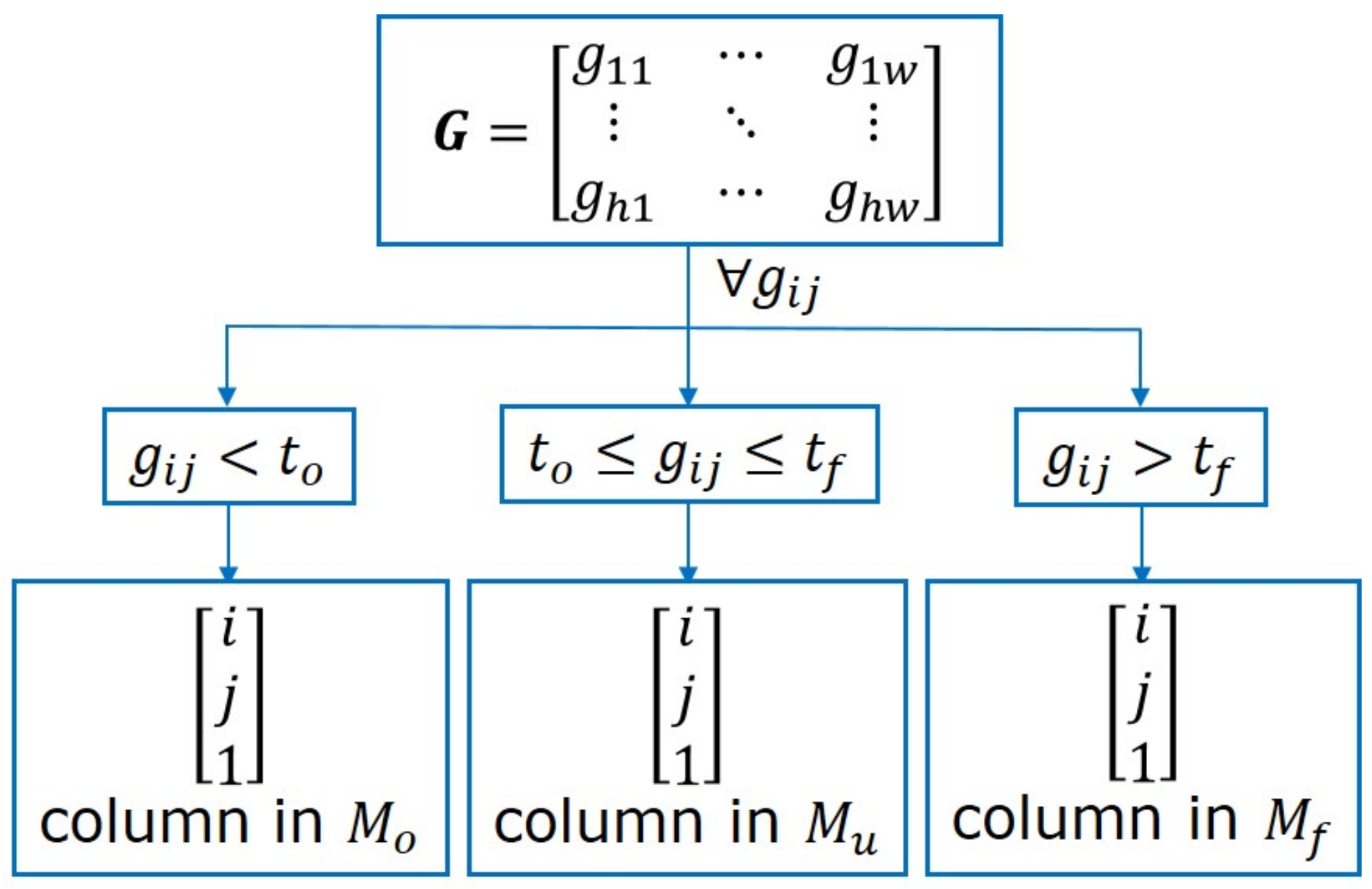
To achieve map calibration, map transformation, including rotation, translation and scaling, will be performed on the original map image. For a gray scale map image of the size , each pixel contains the gray scale value of that pixel. As the gray scale values represent three different occupancy meanings to the robot, we divide the values in matrix to three units, occupied, unknown and free of obstacles, with two thresholds given by and , as shown in Figure 2. Thus, if the gray scale value is lower than , the pixel is occupied. If the gray scale value of the pixel is higher than , the pixel is free of obstacles. Otherwise, the pixel is unknown for the robot.
To present the map transformation method in an intuitive way, we represent the map image as three matrices, , and , containing the pixel coordinates of the gray scale values in the three units mentioned above. The three matrices are of the size , and , respectively, where is the number of pixels that are occupied, is the number of pixels that are unknown to the robot, and is the number of pixels that are free of obstacles, and . The first rows in the three matrices represent the u-coordinate of the pixels, and the second rows represent the v-coordinate of the pixels in the pixel coordinate system. As we use homogeneous coordinates [45] to represent the pixels, all the values in the last rows are assigned ‘1’. The order in which we place the pixel coordinates of the gray scale values in matrix in the occupancy-coordinate matrices is based on checking the gray scale values in row by row and then placing their pixel coordinates into the corresponding matrix.
Map transformation can be directly performed by matrix multiplication on the occupancy-coordinate matrices , and . For example, if the map is supposed to rotate clockwise with angle at the center , enlarge by k times, and then translate , we should firstly translate the origin of the coordinate system to the map center , and the first translation matrix is given by
Subsequently, we should rotate the map clockwise with angle , and the rotation matrix is given by
The next step is to enlarge the image, where the scaling matrix can be described as
Finally, we will translate the origin of the coordinate system back and further translate , and the translation matrix is given by
Therefore, the transformed occupancy-coordinate matrices , and can be obtained by
It is noteworthy that, after we scale up an image, each pixel of the original map image is moved in a certain direction based on the scaling constant k. However, if the scaling factor is larger than 1, there may exist unassigned pixel values in the resultant map image, which are regarded as holes. Furthermore, if the scaling factor is smaller than 1, there will be multiple assigned pixels. Therefore, we will add an interpolation and eight-neighbourhood averaging method after scaling transformation to appropriately assign the gray scale values to these pixels. The details are described in Section 4.3.
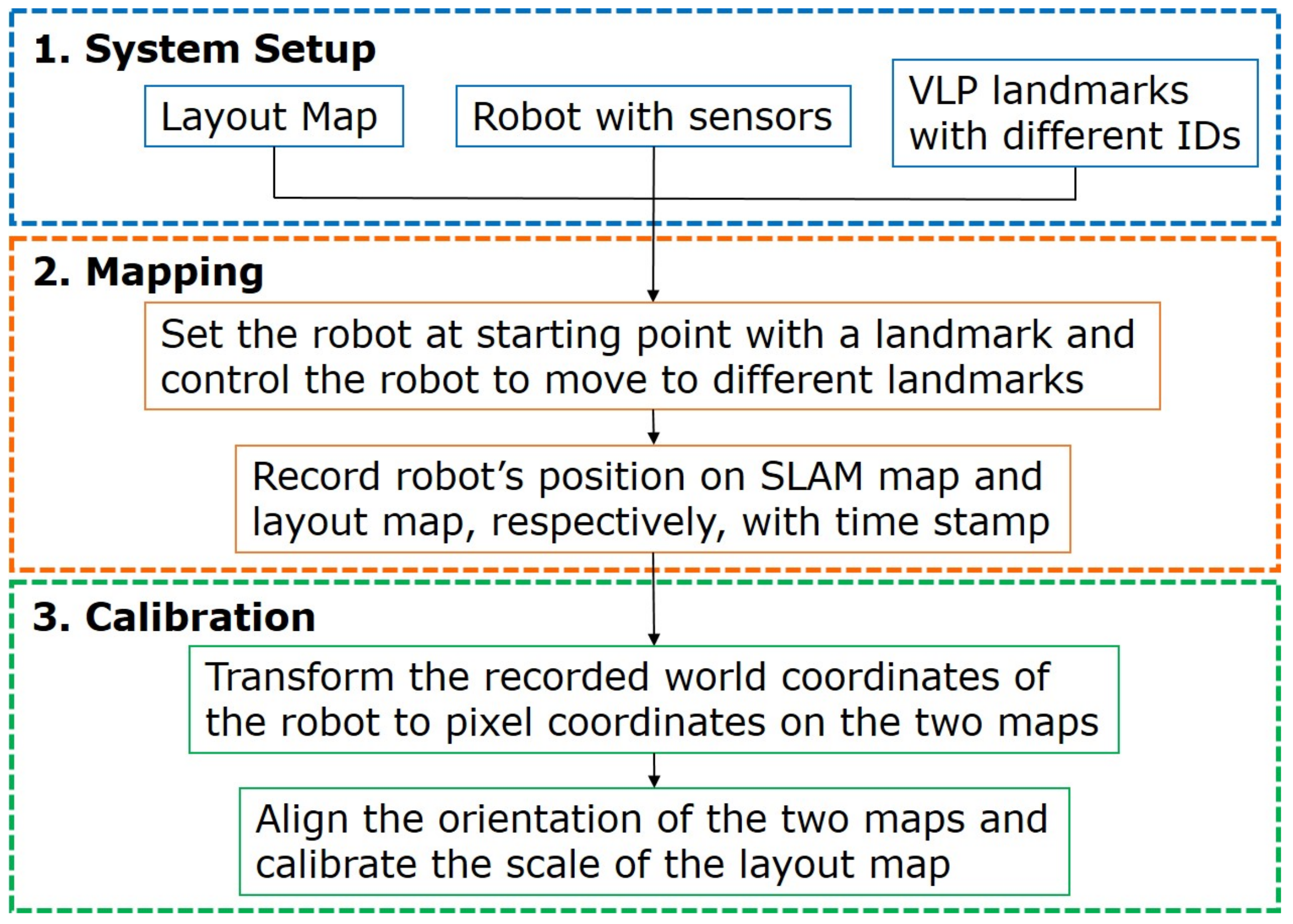
3.3. Overview of the Proposed Map Calibration System
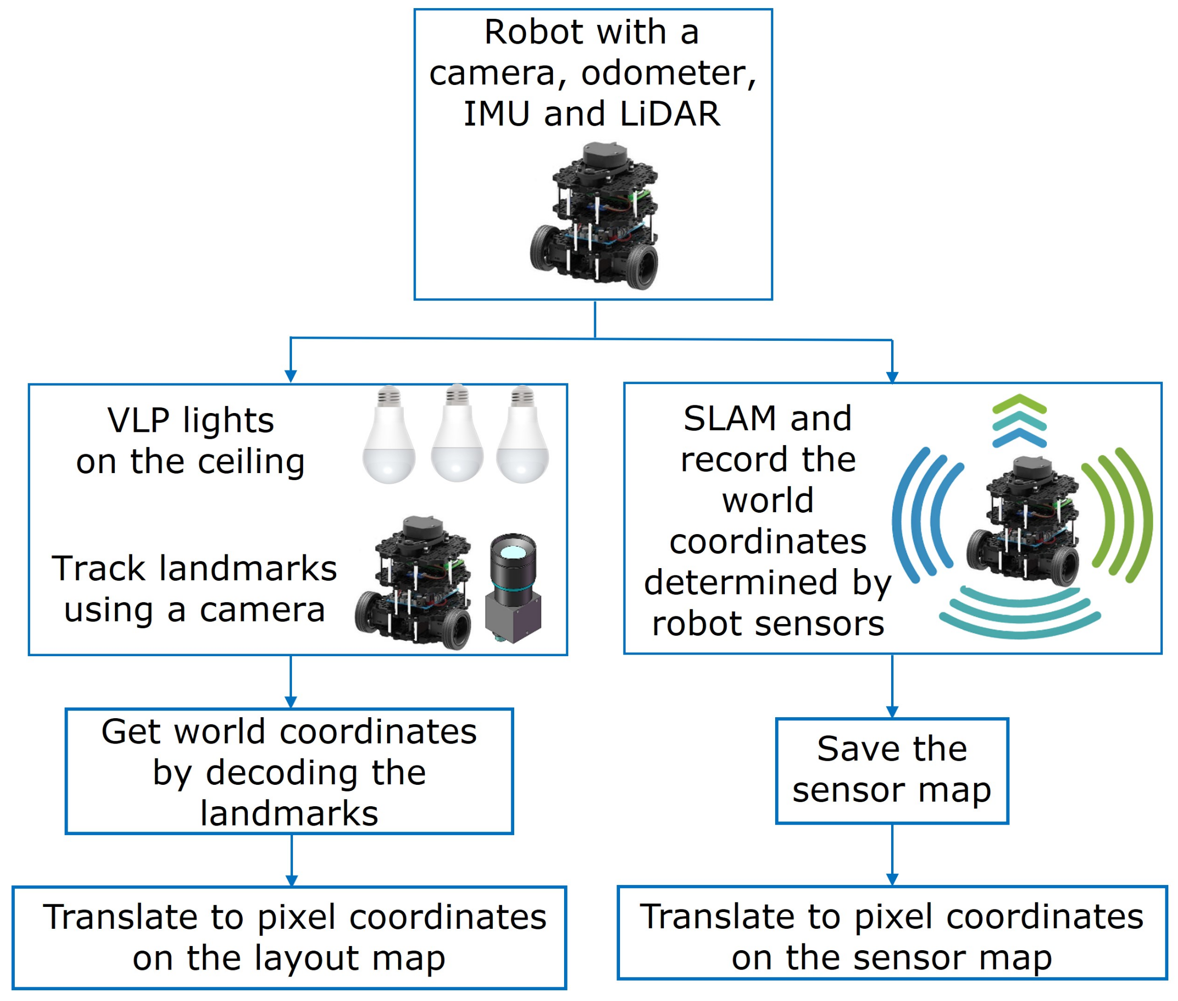
The diagram of the proposed map calibration system using VLP landmarks and SLAM is given in Figure 3. The system setup contains a layout map of the environment to be perceived, a robot, and multiple VLP lights with different IDs installed in the experimental area. The VLP landmarks are mounted on the ceiling and controlled by visible light communication (VLC)-enabled light emitting diode (LED) drivers to transmit optical signals [46]. The LEDs are modulated by the on-off keying scheme and encoded with unique IDs, which contain the LEDs’ world coordinates stored in a uniform resource identifier (URI) database. The robot used in the mapping system is equipped with multiple sensors, including an IMU, odometer and LiDAR. A camera is also mounted on the robot to face toward the ceiling and works in rolling shutter mode to capture the signals broadcast by the VLP-based LEDs, decode and extract the position information [30].
To start the mapping process, the robot is set under a VLP landmark and uses the camera to capture the LED image and decode the position of the starting point. Then, we apply SLAM to the robot and control it to move to different landmarks and record its positions, as acquired from SLAM and VLP landmarks, respectively. The time stamp is simultaneously marked with the position. After the robot has tracked at least two landmarks in the area, the mapping process can be stopped and the occupancy grid map generated by SLAM is saved. Therefore, we obtain one sensor map with the robot’s positions from SLAM and one layout map with the robot’s positions from VLP landmarks. Subsequently, we propose to use the obtained sensor map and the robot’s positions on two maps to calibrate the layout map. Firstly, we transform the recorded world coordinates of the robot to pixel coordinates on the two different maps. Then, we calibrate the layout map by aligning the robot’s positions on it and the occupancy map.
4. Map Calibration Method
In this section, we will describe the details of the proposed VLP landmarks and SLAM-assisted map calibration method. As we mentioned, a layout map contains semantic information, which is readable for humans to give instruction to robots. However, the scale of a layout map may not be accurate, leading to an inaccurate resolution of the map in terms of meters per pixel. In a large scene which is to be perceived, it is difficult and complex to obtain the resolution through measurement. Compared with a layout map, the sensor map generated from SLAM has a much more accurate resolution, but more noise points. Therefore, we propose to calibrate the scale of the layout map, which will help robots to achieve better navigation performance.
4.1. Positioning on Two Different Maps
Figure 4 illustrates the proposed mapping process. At least two VLP landmarks are required to be mounted on the ceiling of the environment which is to be perceived. The exact position of the mounting location in the environment is encoded in the VLP light and is broadcast to the robot by OOK modulation. The positions of the VLP lights are also marked on the layout map. We use a robot equipped with a camera, odometer, IMU and LiDAR. The camera is set to face the ceiling and is used to obtain the robot’s position by VLP. When the camera detects a VLP landmark, it will decode the position information encoded in the rolling shutter patterns, and then translate it to its own position. The translation from the world coordinates of the landmark to the world coordinates of the robot is calculated by the location of the landmark on the camera plane and the orientation of the robot determined by the odometer on the robot. Then, the world coordinates of the robot are further translated to the pixel coordinates on the layout map as the landmarks are labeled on the layout map.
In the mapping process, the robot starts under one of the landmarks to obtain the first key point for map calibration. Then, it is controlled to perceive the environment and conduct SLAM with its odometer, IMU and LiDAR sensors. The world coordinates obtained from the robot sensors are recorded at the same time. After the robot has tracked at least two VLP landmarks, which means that we obtain at least two pairs of coordinates of the key points from the two different positioning methods, we can save the occupancy grid map created by SLAM as a sensor map, set the resolution of the map in terms of meters per pixel, and then translate the recorded world coordinates of the robot to pixel coordinates on the sensor map with the resolution.
4.2. Calibration of the Orientation
A layout map is readable for humans and is always presented in an orientation in which humans can understand the semantic information. However, the sensor map created by the robot may not always be in the same orientation as the layout map used by a human. Therefore, we propose to correct the orientation of the sensor map.
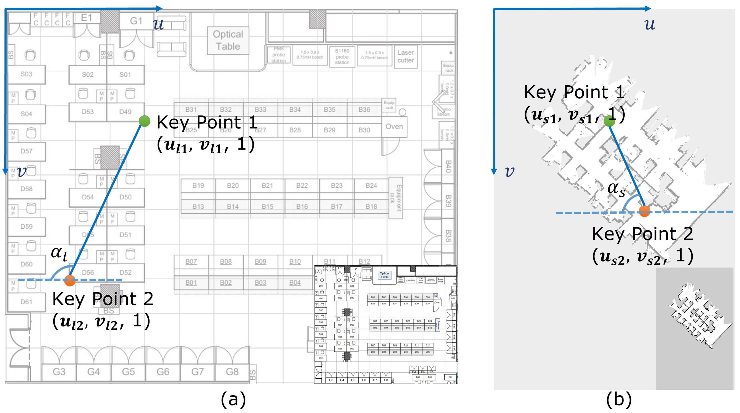
Firstly, we convert the layout map to a gray scale image . Since in a typical layout map, furniture and structures are drawn with black or dark squares. Thus, the gray scale values in the converted layout map have the same meaning as the gray scale values in the sensor map, where if the pixel is in black and its gray scale value is close to 0, the probability of an obstacle at that point is close to 1. Then, for the saved sensor map , we firstly find the occupancy-coordinate representation given by , and . Then, in the mapping process, we assume that the robot has detected two landmarks and labeled them on the two maps according to the translated pixel coordinates given by (,,1) and (,,1) on the layout map and (,,1) and (,,1) on the sensor map, as shown in Figure 5. Then, we draw a line between the two key points and find the angle between the line and the negative u-axis in the pixel coordinate system.
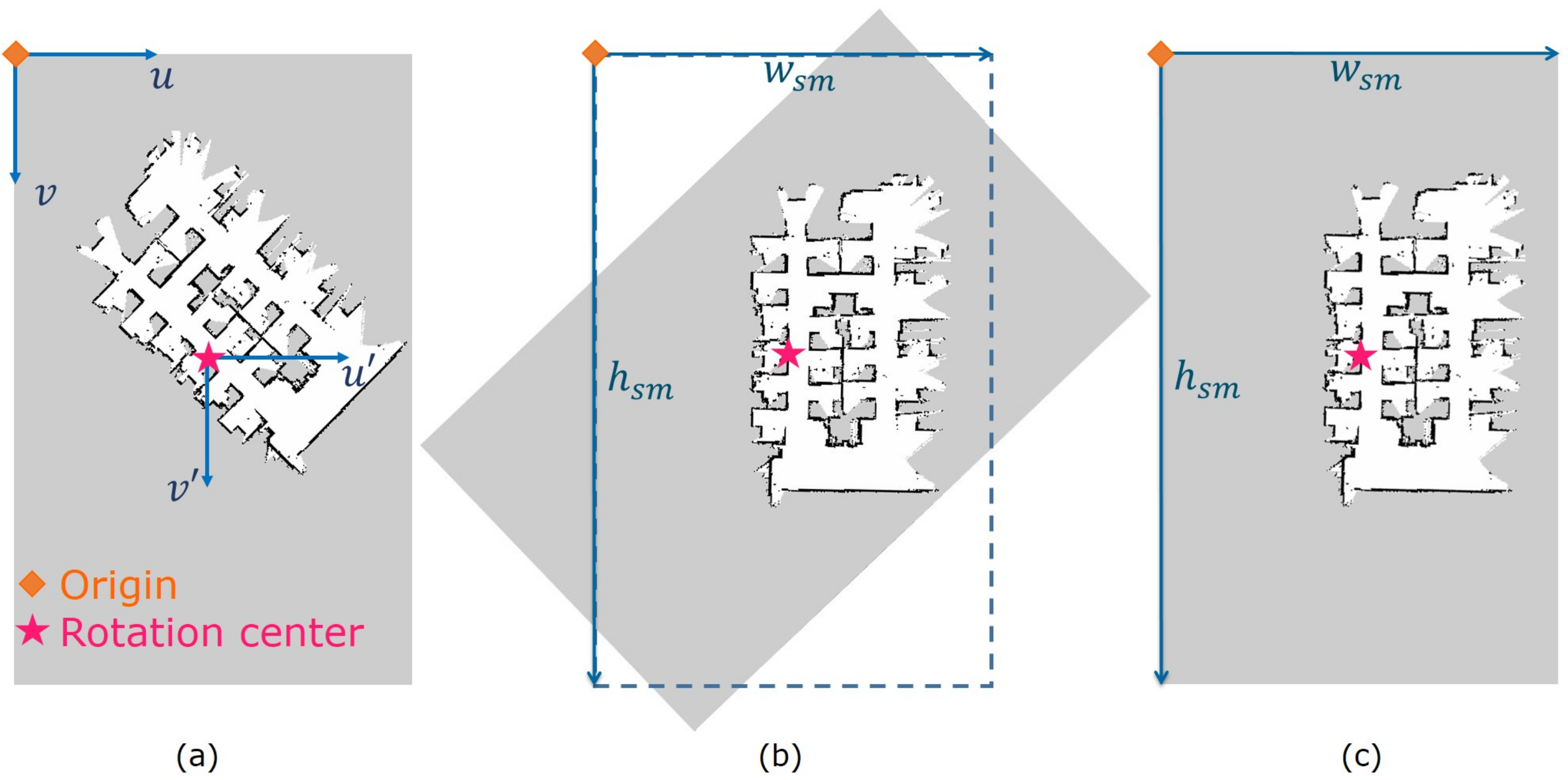
To rotate the sensor map clockwise with the angle of , where is the angle on the layout map and is the angle on the sensor map, we firstly translate the origin of the coordinate system to the map center , which is the rotation center, as shown in Figure 6a. The origin translation matrix is given by
where and are the width and height of the sensor map image . Subsequently, we substitute the rotation angle into the rotation matrix defined in (3) as
Then, we translate the origin of the coordinate system back, and the translation matrix is given by
By multiplying the translation matrices and rotation matrix, the occupancy-coordinate representation matrices of the sensor map are given by
where , and are the occupancy-coordinate matrices after rotation. Then, we assign the corresponding gray scale values to the pixels in sensor map image and obtain the rotated sensor map image .
After rotation, the rotated sensor map image may not be in the original size of the sensor map image given by . Therefore, we find the maximal u-coordinate of the pixels indicating the cells are free of obstacles or occupied by an obstacle, which is given by
where is the integer set, is the width of matrix and is the width of matrix . Similarly, we determine the maximal v-coordinate of the pixels indicating the cells are free of obstacles or occupied by an obstacle, which is given by
Then, we find the maximum in the u-coordinates and v-coordinates, respectively, given by
where (, ) is the size to which we will crop the rotated sensor map.
Then, we trim the map image by the width of and the height of , as shown in Figure 6b and delete those columns in , and . Furthermore, we fill in the corners with the grayvalues indicating that the pixel is unknown, namely, the half probability of an obstacle, as shown in Figure 6c, and add the pixel coordinates of the elements in the corners to matrix . The obtained occupancy-coordinate matrices of the sensor map after cropping and filling are given by , and .
It is noteworthy that the map rotation process we describe above is based on two key points, namely, two VLP landmarks, but it is scalable to a perceived environment that is mounted with multiple landmarks by computing the average rotation angle of every two key points on the map and substituting the average angle into (8).
4.3. Calibration of the Scale
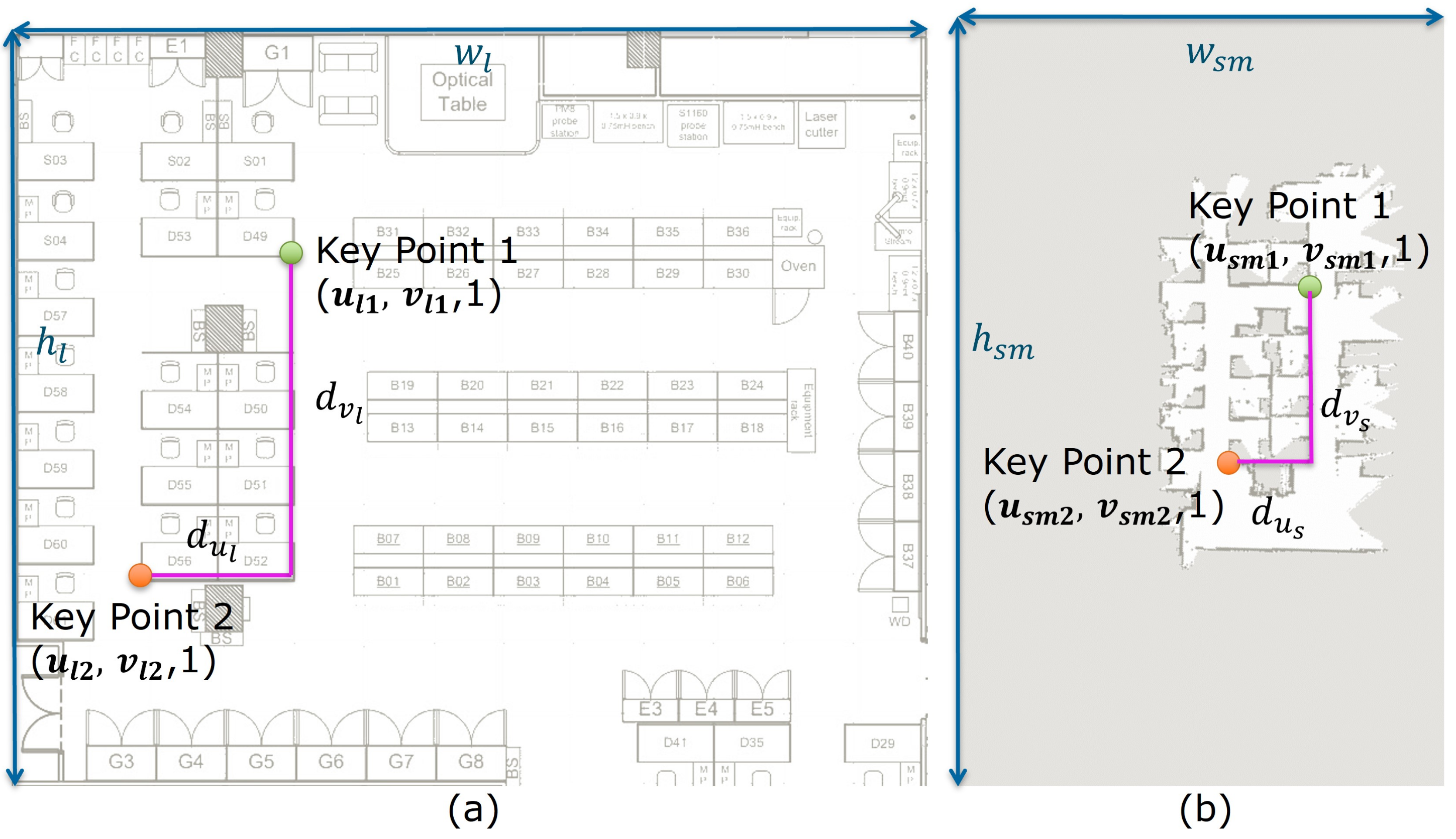
After we align the orientation of the two maps, the next step is to align their scales. As the resolution of the sensor map obtained from SLAM is more accurate than that of a manually drawn map, we propose to calibrate the scale of the layout map with the sensor map. Firstly, we determine the occupancy-coordinate representation of the layout map matrix given by , and , which indicate the pixels are occupied, unknown or free of obstacles, respectively. Then, we find the pixel distance between the two key points on the layout map, given by in the u-axis and in the v-axis, as shown in Figure 7a, where is the width and is the height of the layout map. Similarly, we obtain the pixel distance between the two key points on the sensor map, given by in the u-axis and in the v-axis, as shown in Figure 7b. It is noteworthy that, according to (10a), the pixel coordinates of the two key points on the sensor map have also been transformed after the rotation as
where (, ,1) and (, ,1) are the pixel coordinates of the key points on the sensor map after rotation.
Next, we modify the scale of the layout map, and the scaling matrix is given by
Then, we multiply matrix with the occupancy-coordinate representation matrices of the layout map as
where , and are the occupancy-coordinate layout map matrices after scaling.
Since the scaling factor may not be an integer, the obtained pixel coordinates in the layout map matrices , and may result in non-integers. Therefore, we firstly round all the values in , as given by
where is the floor function, , , is the width of matrix and denotes the natural number set. Similarly, we round the values in and .
In addition, if the scaling factor is smaller than 1, after multiplying the scaling matrix, there will be multiple columns in composed of the same pixel coordinates. Then, for each occupancy-coordinate matrix, we treat each column as a single entity and extract the unique columns with no repetitions. The extracted columns constitute three new matrices given by , and . Furthermore, one pair of pixel coordinates may occur in different occupancy-coordinate matrices, indicating different gray scale values in the layout map image. To keep the consistency of the gray scale values in the map image, we propose to use the eight-neighborhood averaging method to determine the gray scale value of a pixel that has multiple correspondences. For example, if pixel coordinates (, ,1) occur in both of the first two columns of matrix and , we check the eight neighborhood pixels (, ,1), where = 1, 0, −1, find the average of the gray scale values that these pixel coordinates refer to, and assign the average value to pixel (, ,1) given by . Then, coordinates (, ,1) are reallocated to the occupancy-coordinate matrix by comparing with the threshold and , and are removed from previous matrices and .
Moreover, if the scaling factor is larger than 1, there will exist unassigned pixels in the map image after scaling, which are regarded as holes. To maintain a consistent trend across the pixels, we propose to use a bilinear interpolation method to appropriately assign the gray scale values to these pixels by at least four well-assigned pixels. For example, the gray scale value of pixel (, , 1) is unassigned, but the gray scale values at the pixels (, ,1), (, ,1), (, ,1) and (, ,1) are known. We first perform the linear interpolation in the u-coordinates as
where , , and are the gray scale values of pixel (, ,1), (, ,1), (, ,1) and (, ,1), respectively. Then, we proceed by interpolating in the v-coordinates and substituting the results of and from (18) as
Using (19), each unassigned pixel can be determined by at least four pixels allocated with definite gray scale values. Thereby, after multiplying a scaling matrix, a complete map image can be obtained by a rounding operation, eliminating duplication, eight-neighborhood averaging and bilinear interpolation.
Furthermore, similarly to the calibration method for the map orientation described in Section 4.2, the calibration for scale is also scalable to the a perceived environment that contains multiple VLP landmarks, as long as we find the average of the scaling factor of every two key points on the map and substitute the average into (15).
5. Experimental Results
In this section, experiments are conducted to evaluate the performance of the proposed map calibration method. We will describe the experiment setup, evaluate map alignment performances and analyze the navigation results on the maps that are calibrated by the proposed method.
5.1. Experiment Setup
The experiment is performed in our lab (Integrated Circuit Design Center, 3/F, CYT Building, HKUST). Two maps with different levels of accuracy are prepared: one is a building blueprint with a high accuracy and the other is a floor map with a rough accuracy, as shown in Figure 8a,b. We set three VLP lights as landmarks at different locations in the perceived environment, as illustrated in Figure 8c. They are modulated with different IDs, which are encoded with different positioning information stored in the database. Figure 8d illustrates the TurtleBot3 Burger robot, the ROS standard platform robot we use for the VLP receiver and SLAM process. The robot is equipped with a Raspberry Pi 3 Model B, running Ubuntu 16.04 with ROS. Sensors are mounted on the robot for the SLAM process and VLP decoding. These include an IMU, odometer, 360° LiDAR and an industrial camera facing toward the ceiling. We use a laptop running Ubuntu 18.04 with ROS to remote control the robot and record the data from the robot in the mapping process. The experimental parameters and the camera options are summarized in Table 1.
5.2. Mapping Process and Alignment Results
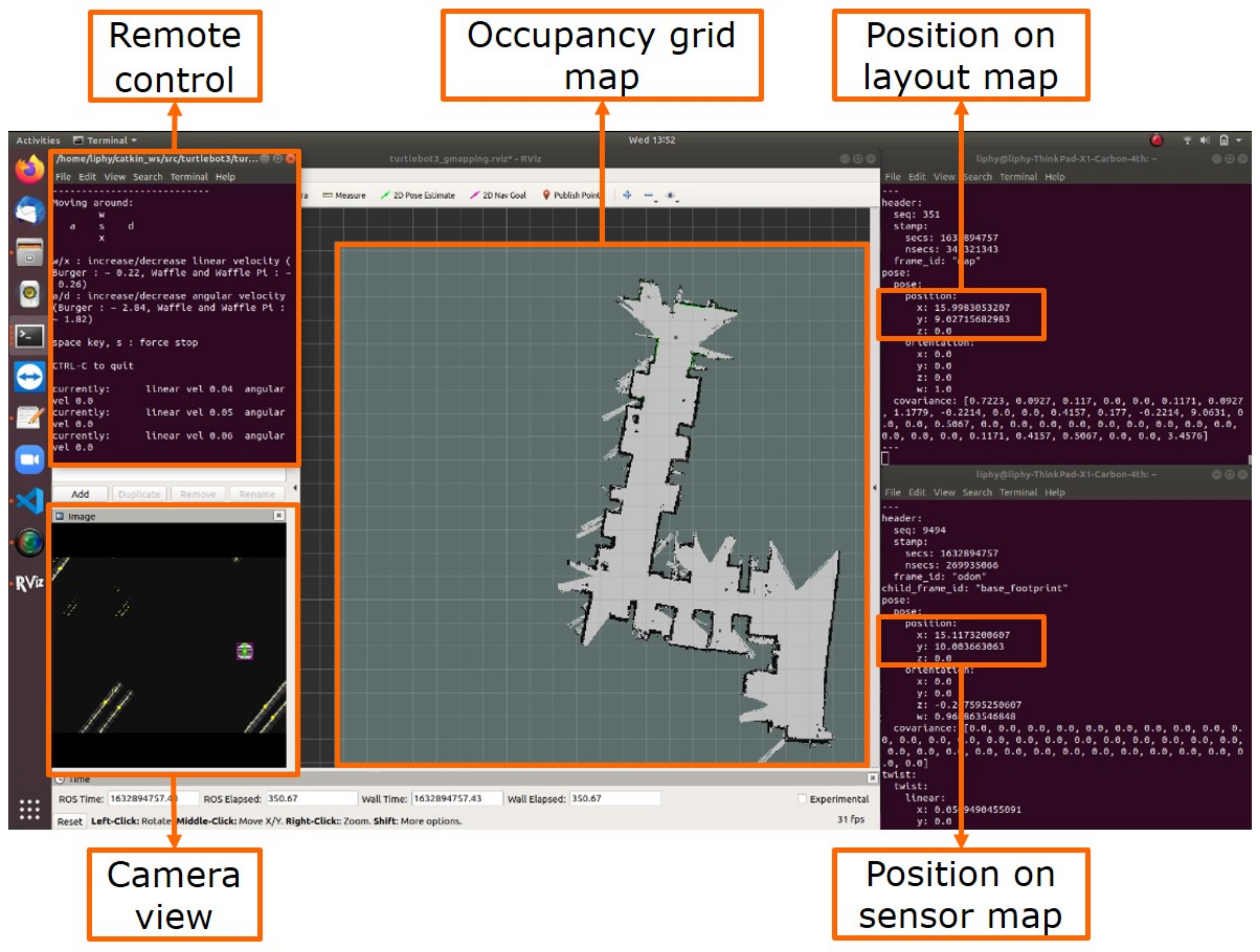
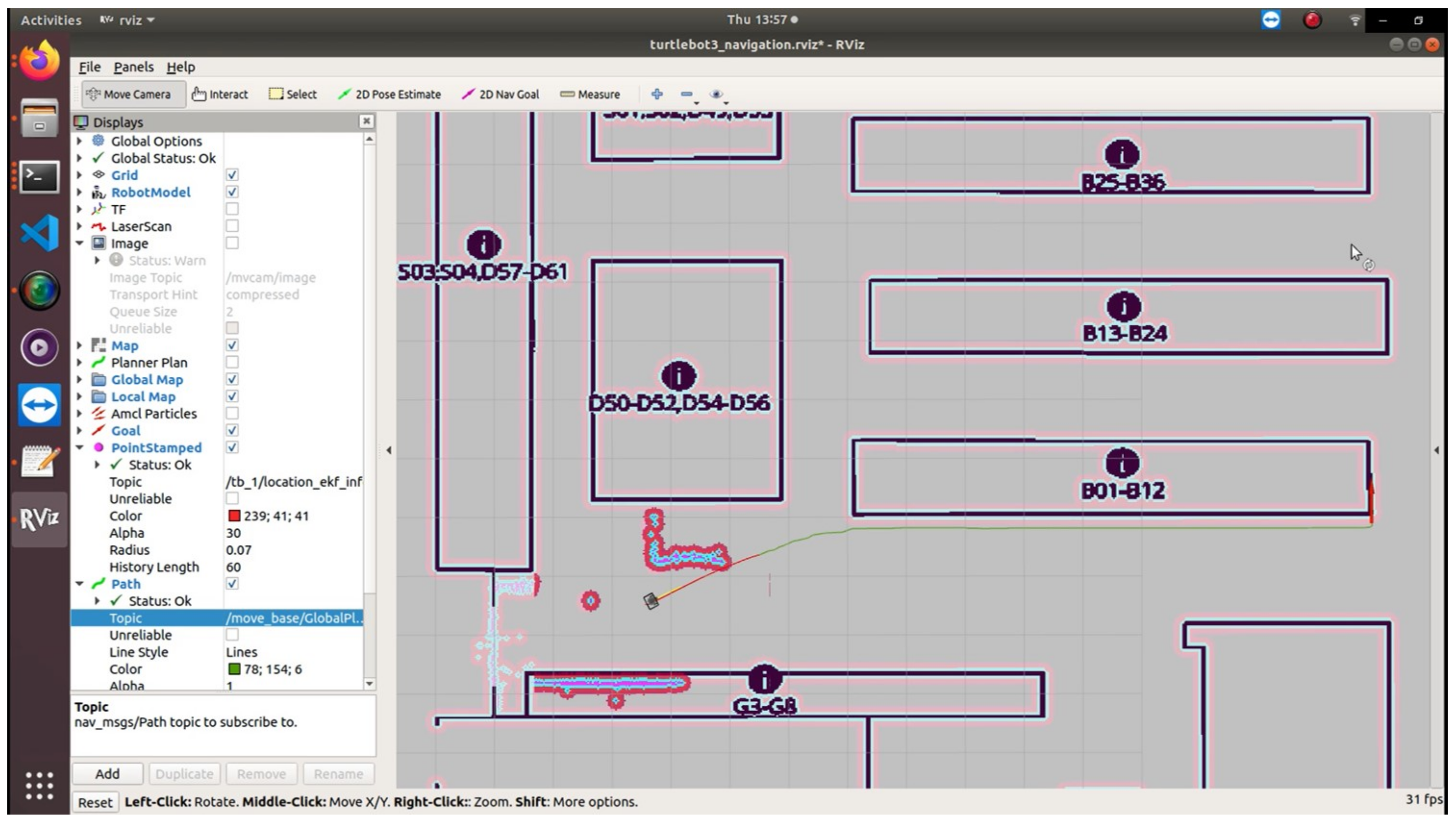
In the mapping experiment, we set the robot under VLP light No. 1 as the starting point and control it to move to VLP light No. 2 and then No. 3. At the same time, the robot performs SLAM using the Gmapping [44] package in ROS. Thus, the robot’s location on the SLAM map and position as estimated by the VLP system are recorded synchronously, and the SLAM map is visualized in RViz software on the laptop, as shown in Figure 9. After the robot has tracked all three VLP lights, the occupancy grid map is saved. Then, we perform the proposed map calibration method to calibrate the orientation and scale of the saved sensor map and the building blueprint. To intuitively evaluate the performance of the map calibration results, we align the two maps, specifically, translating the key points to the same pixels on the map. Then, we overlap the pixels which are occupied to compare the structures shown on different maps of the same experimental area.
By multiplying the scaling matrix as (15) and rounding the values, the pixel coordinates of the key points on the layout map after scaling can be computed as (, ) and (, ). Then, we translate the pixels on the sensor map so that the key points on the two maps are located at the same pixel coordinates. The translation matrix is given by
Multiplying the translation matrix in (20), the translated matrices are given by
Then, we find all the pixels on the layout map, whose coordinates are given in , and allocate these pixels with the gray scale values of the same pixels on the sensor map.
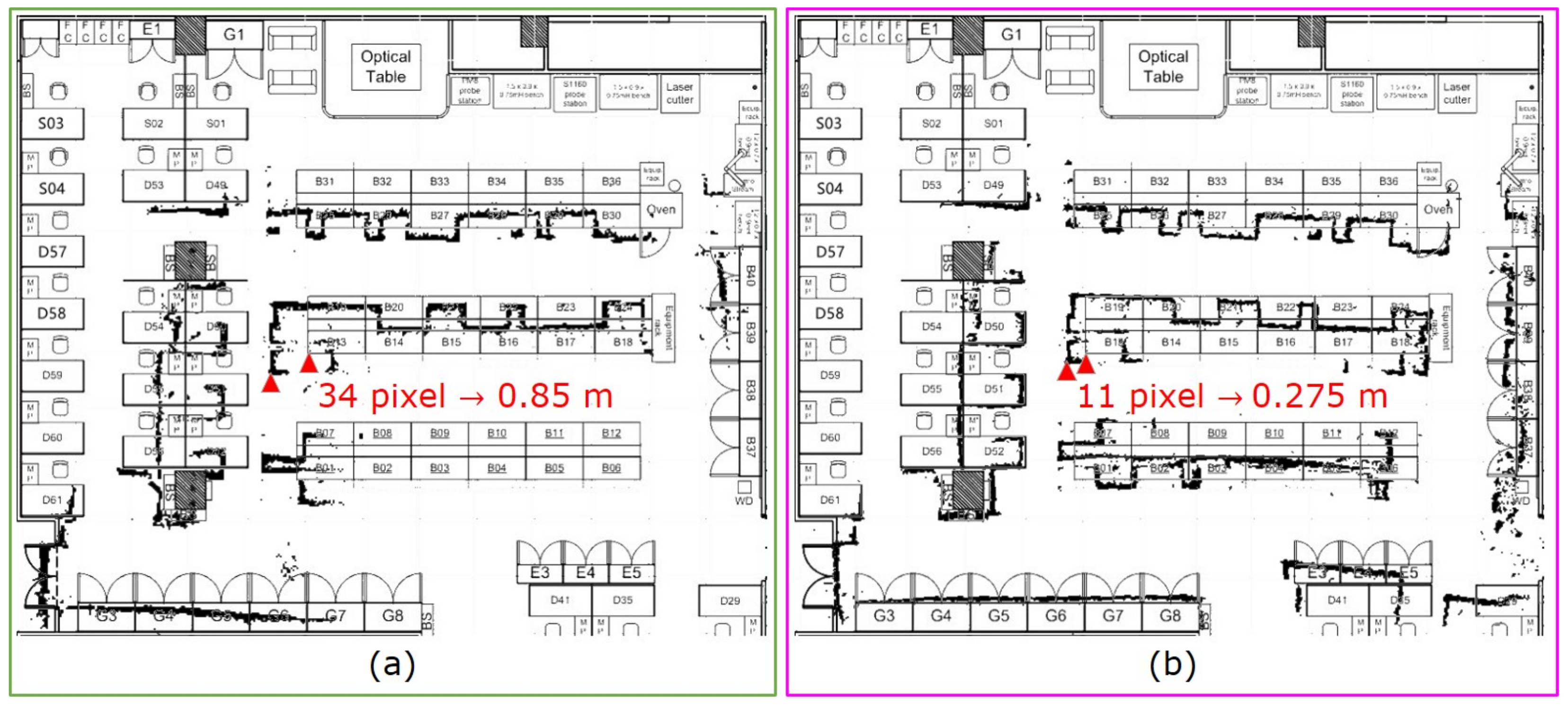
We first calibrate the building blueprint as shown in Figure 8a, with two key points given by VLP lights No.1 and No.3. The alignment result is shown in Figure 10a, and we check the pixel distance between the left bottom corners of cubicle B13 on the two maps given by 34 pixels. By multiplying the resolution of the map in terms of meters per pixel, the distance is 0.85 m in the world coordinate system. To improve the alignment performance, we further add one key point given by VLP light No.2 by determining the rotation angle and scaling factor with the average of every two key points. The alignment result based on three key points is illustrated in Figure 10b, and the distance between the left bottom corners of cubicle B13 is given by 11 pixels in the pixel coordinate system and 0.275 m in the world coordinate system. Therefore, increasing one key point in the mapping process will improve the map alignment performance. In the next section, to achieve better navigation performance, we use the layout maps calibrated with three key points.
5.3. Navigation on Calibrated Map
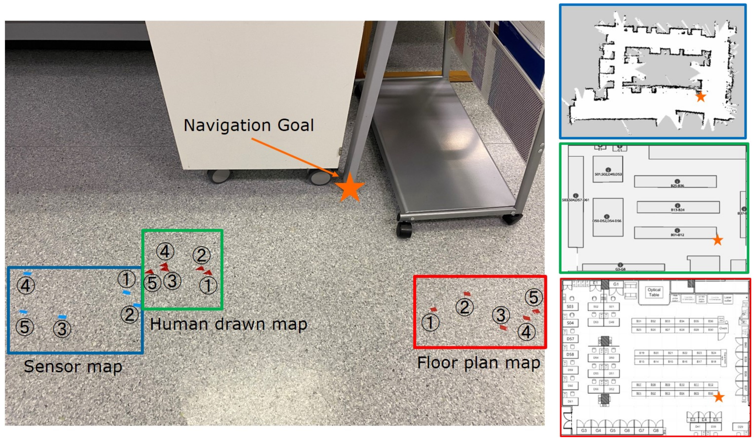
To further evaluate the performance of the proposed map calibration method, we use a navigation system based on an adaptive Monte Carlo localization (AMCL) [47] package, Dijkstra’s algorithm [48] package and dynamic window approach (DWA) [49] package in ROS to achieve autonomous navigation of the robot on the calibrated maps. We set the navigation goal of the robot to be next to cubicle B06, as shown in Figure 11. The distance between the starting point and the target point is 14.14 m. During the navigation, the position of the robot is determined by the AMCL method. The global plan is achieved by Dijkstra’s algorithm, and the local plan is designed by the DWA planner. As shown in Figure 12, the blue dots encapsulated in the outlines in pink are the obstacles detected by the LiDAR on the robot. The red line is the DWA local planner, and the green line, which connects to the navigation goal, represented by a red arrow, is the global plan based on Dijkstra’s algorithm. On each map, we repeat the navigation five times and the navigation results on the different maps are illustrated in Figure 11 and summarized in Table 2. The table lists the distance between the actual point reached in the real world and the target destination sent to the robot. Compared with the navigation results on the sensor map, those on the calibrated building blueprint and the calibrated floor map are much closer to the set destination. The average navigation accuracy is improved by 24.6 cm on the building blueprint and 22.6 cm on the floor map, respectively. Furthermore, with the proposed calibration method, the robot on the floor map, which has lower accuracy in scale and structure location than the building blueprint, can achieve a navigation performance nearly as good as that on the building blueprint, which verifies the effectiveness of the proposed map calibration method.
5.4. Navigation with Semantic Information
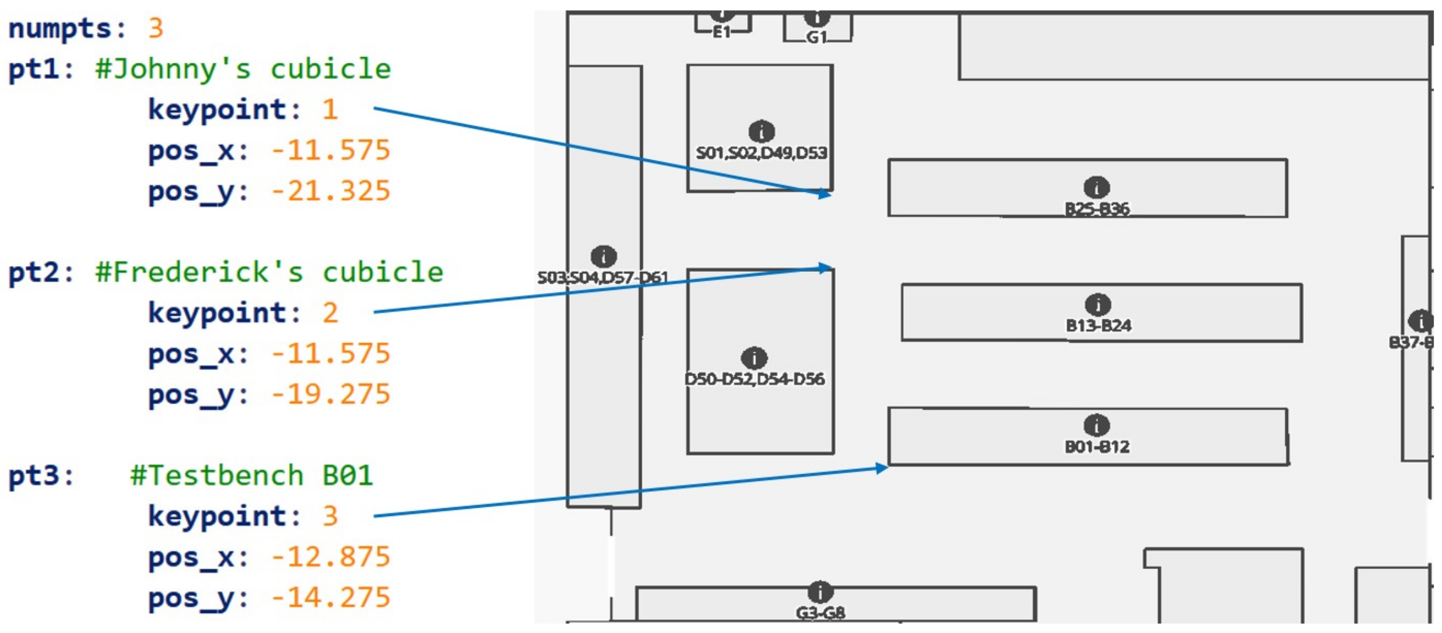
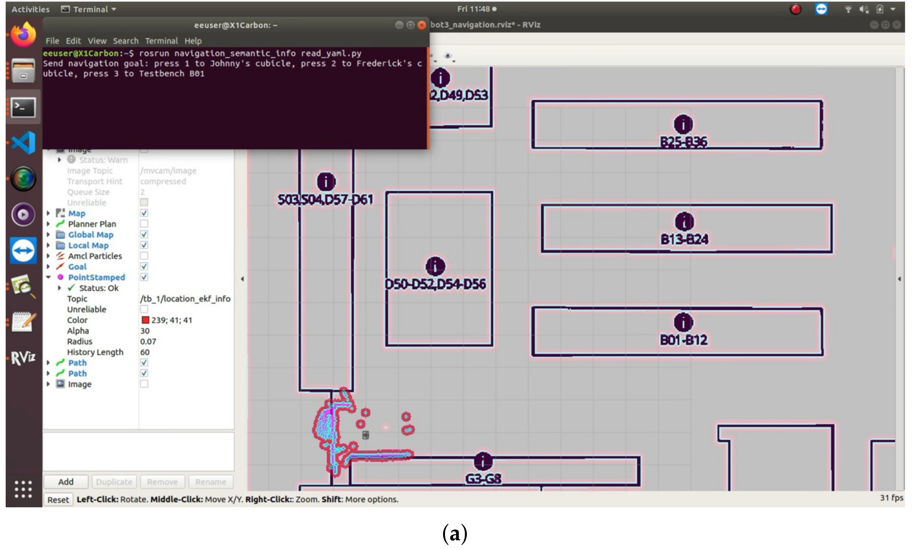
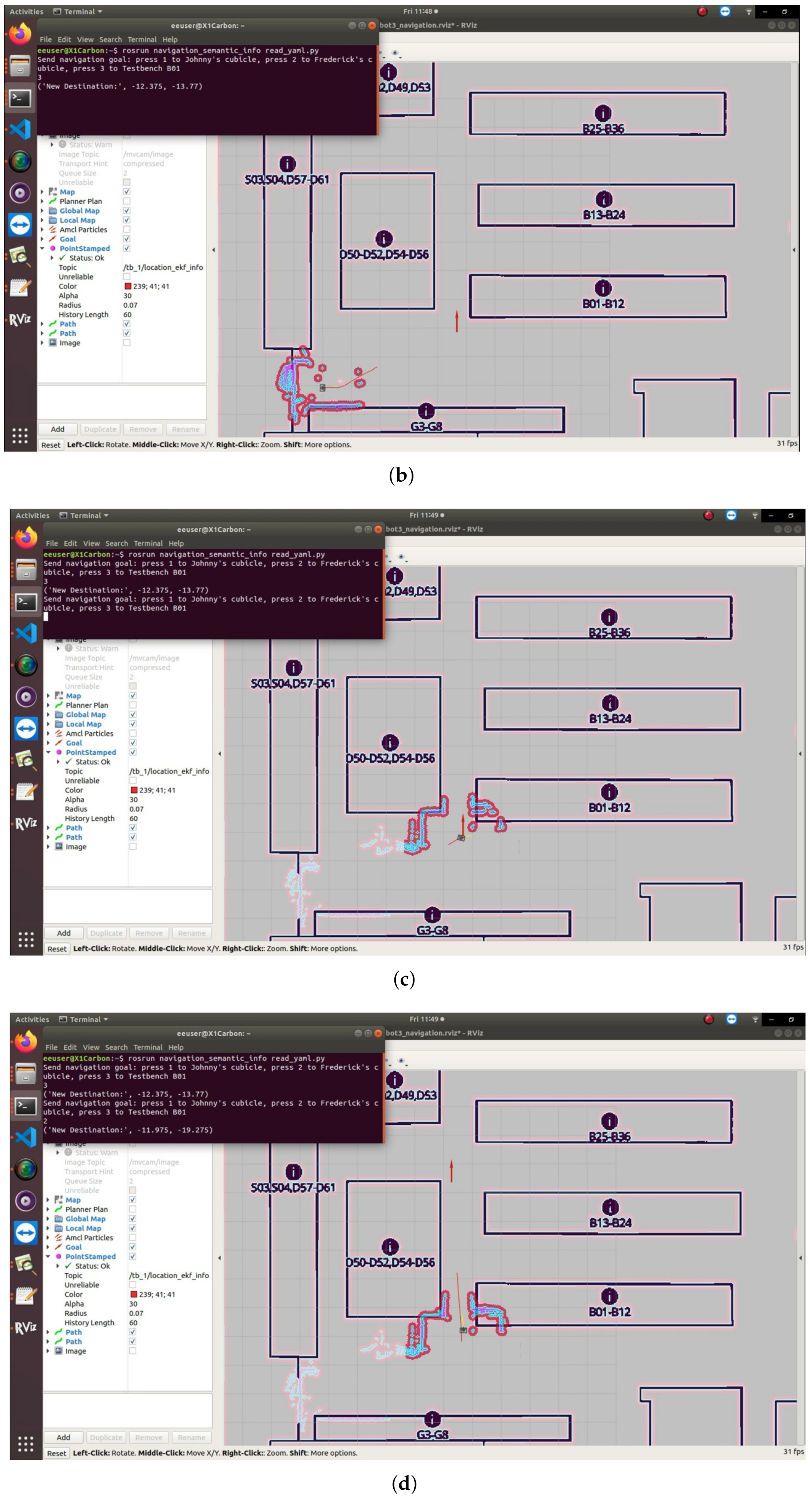
As we mentioned in Section 1, a layout map contains semantic information which is accessible to humans and allows them to send instructions to robots. After calibrating the layout map, we can not only send the navigation target to the robot by selecting one point on the map, but also navigate the robot with pre-compiled semantic information on the layout map. For the floor map illustrated in Figure 8b, we compile three positions with semantic information, as shown in Figure 13, where D49 refers to Johnny’s cubicle, D50 refers to Frederick’s cubicle and B01 refers to the last line of the test bench. Figure 14 illustrates the navigation experiment with semantic information. When the program starts, the semantic information of the map is shown in the terminal, as shown in Figure 14a. Then, we send a navigation goal by tapping the target identifier number of the semantic information, and a red arrow indicating the aimed point is marked on the floor map, as shown in Figure 14b. Figure 14c illustrates the condition that the robot has arrived at the target point and the semantic information is illustrated again in the terminal. We can repeat the navigation process by tapping another identifier number of the navigation goal, as shown in Figure 14d. Using this process, the semantic information on the floor map helps humans to set tasks for the robots in a more straightforward and user-friendly way compared with a sensor map, which has no semantic information.
6. Conclusions and Future Work
In this paper, we propose a VLP landmark and SLAM-assisted automatic map calibration method for robot navigation. VLP landmarks with different IDs are mounted in the environment to be perceived, and a layout map of the environment is prepared to be calibrated. By tracking the landmarks and conducting SLAM at the same time, the robot’s position as obtained from the VLP method and the position as obtained from SLAM are recorded synchronously with the time stamp. By aligning the recorded coordinates on the layout map and the sensor map saved from SLAM, the orientation and the scale of the layout map is calibrated. Experiments are performed to evaluate the proposed map calibration system in terms of the map alignment performance and navigation performance. We calibrate two layout maps: a building blueprint of high accuracy and a floor map of rough accuracy. The experiment results show that the robot can achieve a better navigation performance on the calibrated layout maps compared with that on the sensor map, and can achieve the navigation performance on the calibrated floor map almost the same as that on the calibrated building blueprint.
In this paper, VLP landmarks are used in map calibration for robot navigation. In the future work, a VLP landmark-aided SLAM system can be developed by inducing VLP landmark to SLAM system to correct the distortion of the occupancy grid map caused by the odometer, as the absolute positioning result from VLP lights can help increase localization accuracy. Furthermore, if we already have an accurate layout map, the gray scale values on the layout map can provide the prior information for LiDAR detection and correct the distortion caused by the odometer as well.
Author Contributions
All authors contributed to the study conception and design. Experiments and data analysis were performed by Y.W. and B.H. The first draft of the manuscript was written by Y.W. All authors have read and agreed to the published version of the manuscript.
Funding
This work was supported in part by the Foshan-HKUST Project, Government of Foshan municipality under the project FSUST20-SHCIRI06C and in part by the Hong Kong Research Grants Council under General Research Fund (GRF) project no. 16200419.
Institutional Review Board Statement
Not applicable.
Informed Consent Statement
Not applicable.
Data Availability Statement
Not applicable.
Conflicts of Interest
The authors declare no conflict of interest.
References
- Su, H.; Qi, W.; Schmirander, Y.; Ovur, S.E.; Cai, S.; Xiong, X. A human activity-aware shared control solution for medical human–robot interaction. Assem. Autom. 2022, 42, 388–394. [Google Scholar] [CrossRef]
- Qi, W.; Ovur, S.E.; Li, Z.; Marzullo, A.; Song, R. Multi-sensor guided hand gesture recognition for a teleoperated robot using a recurrent neural network. IEEE Robot. Autom. Lett. 2021, 6, 6039–6045. [Google Scholar] [CrossRef]
- Liu, C.; Tomizuka, M. Algorithmic safety measures for intelligent industrial co-robots. In Proceedings of the 2016 IEEE International Conference on Robotics and Automation (ICRA), Stockholm, Sweden, 16–21 May 2016; pp. 3095–3102. [Google Scholar]
- Peternel, L.; Kim, W.; Babič, J.; Ajoudani, A. Towards ergonomic control of human-robot co-manipulation and handover. In Proceedings of the 2017 IEEE-RAS 17th International Conference on Humanoid Robotics (Humanoids), Birmingham, UK, 15–17 November 2017; pp. 55–60. [Google Scholar]
- Zhuang, Y.; Hua, L.; Qi, L.; Yang, J.; Cao, P.; Cao, Y.; Wu, Y.; Thompson, J.; Haas, H. A survey of positioning systems using visible LED lights. IEEE Commun. Surv. Tutor. 2018, 20, 1963–1988. [Google Scholar] [CrossRef] [Green Version]
- Guan, W.; Huang, L.; Hussain, B.; Yue, C.P. Robust robotic localization using visible light positioning and inertial fusion. IEEE Sens. J. 2021, 22, 4882–4892. [Google Scholar] [CrossRef]
- Wang, Y.; Hussain, B.; Yue, C.P. Arbitrarily Tilted Receiver Camera Correction and Partially Blocked LED Image Compensation for Indoor Visible Light Positioning. IEEE Sens. J. 2021, 22, 4800–4807. [Google Scholar] [CrossRef]
- Gao, H.; Zhang, X.; Yuan, J.; Song, J.; Fang, Y. A novel global localization approach based on structural unit encoding and multiple hypothesis tracking. IEEE Trans. Instrum. Meas. 2019, 68, 4427–4442. [Google Scholar] [CrossRef]
- Huletski, A.; Kartashov, D.; Krinkin, K. VinySLAM: An indoor SLAM method for low-cost platforms based on the transferable belief model. In Proceedings of the 2017 IEEE/RSJ International Conference on Intelligent Robots and Systems (IROS), Vancouver, BC, Cannada, 24–28 September 2017; pp. 6770–6776. [Google Scholar]
- Cadena, C.; Carlone, L.; Carrillo, H.; Latif, Y.; Scaramuzza, D.; Neira, J.; Reid, I.; Leonard, J.J. Past, present, and future of simultaneous localization and mapping: Toward the robust-perception age. IEEE Trans. Robot. 2016, 32, 1309–1332. [Google Scholar] [CrossRef] [Green Version]
- Kshirsagar, J.; Shue, S.; Conrad, J.M. A Survey of Implementation of Multi-Robot Simultaneous Localization and Mapping. In Proceedings of the SoutheastCon 2018, St. Petersburg, FL, USA, 19–22 April 2018; pp. 1–7. [Google Scholar]
- Bresson, G.; Alsayed, Z.; Yu, L.; Glaser, S. Simultaneous localization and mapping: A survey of current trends in autonomous driving. IEEE Trans. Intell. Transp. Syst. 2017, 2, 194–220. [Google Scholar] [CrossRef] [Green Version]
- Tan, H.; Song, J. Design of An Intelligent Transfer Robot with Color Recognition. In Proceedings of the 2021 3rd International Conference on Applied Machine Learning (ICAML), Chengdu, China, 14–16 May 2021; pp. 287–291. [Google Scholar]
- Patil, A.; Bae, J.; Park, M. An Algorithm for Task Allocation and Planning for a Heterogeneous Multi-Robot System to Minimize the Last Task Completion Time. Sensors 2022, 22, 5637. [Google Scholar] [CrossRef]
- Guo, Y.; Yang, Y.; Liu, Y.; Li, Q.; Cao, F.; Feng, M.; Wu, H.; Li, W.; Kang, Y. Development Status and Multilevel Classification Strategy of Medical Robots. Electronics 2021, 10, 1278. [Google Scholar] [CrossRef]
- Khan, Z.H.; Siddique, A.; Lee, C.W. Robotics utilization for healthcare digitization in global COVID-19 management. Int. J. Environ. Res. Public Health 2020, 17, 3819. [Google Scholar] [CrossRef]
- Kostavelis, I.; Kargakos, A.; Skartados, E.; Peleka, G.; Giakoumis, D.; Sarantopoulos, I.; Agriomallos, I.; Doulgeri, Z.; Endo, S.; Stüber, H.; et al. Robotic Assistance in Medication Intake: A Complete Pipeline. Appl. Sci. 2022, 12, 1379. [Google Scholar] [CrossRef]
- Iqbal, J.; Xu, R.; Sun, S.; Li, C. Simulation of an autonomous mobile robot for LiDAR-based in-field phenotyping and navigation. Robotics 2020, 9, 46. [Google Scholar] [CrossRef]
- Santos, L.; Santos, F.; Mendes, J.; Costa, P.; Lima, J.; Reis, R.; Shinde, P. Path planning aware of robot’s center of mass for steep slope vineyards. Robotica 2020, 38, 684–698. [Google Scholar] [CrossRef]
- Al Khatib, E.I.; Jaradat, M.A.K.; Abdel-Hafez, M.F. Low-cost reduced navigation system for mobile robot in indoor/outdoor environments. IEEE Access 2020, 8, 25014–25026. [Google Scholar] [CrossRef]
- Lv, W.; Kang, Y.; Qin, J. Indoor localization for skid-steering mobile robot by fusing encoder, gyroscope, and magnetometer. IEEE Trans. Syst. Man Cybern. Syst. 2017, 49, 1241–1253. [Google Scholar] [CrossRef]
- Murata, Y.; Murakami, T. Estimation of Posture and Position Based on Geometric Calculation Using IMUs. In Proceedings of the IECON 2019-45th Annual Conference of the IEEE Industrial Electronics Society, Lisbon, Portugal, 14–17 October 2019; Volume 1, pp. 5388–5393. [Google Scholar]
- McGregor, A.; Dobie, G.; Pearson, N.R.; MacLeod, C.N.; Gachagan, A. Determining position and orientation of a 3-wheel robot on a pipe using an accelerometer. IEEE Sens. J. 2020, 20, 5061–5071. [Google Scholar] [CrossRef]
- Da Mota, F.A.; Rocha, M.X.; Rodrigues, J.J.; De Albuquerque, V.H.C.; De Alexandria, A.R. Localization and navigation for autonomous mobile robots using Petri nets in indoor environments. IEEE Access 2018, 6, 31665–31676. [Google Scholar] [CrossRef]
- Zhang, J.; Lyu, Y.; Patton, J.; Periaswamy, S.C.; Roppel, T. BFVP: A probabilistic UHF RFID tag localization algorithm using Bayesian filter and a variable power RFID model. IEEE Trans. Ind. Electron. 2018, 65, 8250–8259. [Google Scholar] [CrossRef]
- Su, D.; Kong, H.; Sukkarieh, S.; Huang, S. Necessary and Sufficient Conditions for Observability of SLAM-Based TDOA Sensor Array Calibration and Source Localization. IEEE Trans. Robot. 2021, 37, 1451–1468. [Google Scholar] [CrossRef]
- Naab, C.; Zheng, Z. Application of the unscented Kalman filter in position estimation a case study on a robot for precise positioning. Rob. Auton. Syst. 2022, 147, 103904. [Google Scholar] [CrossRef]
- Schouten, G.; Steckel, J. A biomimetic radar system for autonomous navigation. IEEE Trans. Robot. 2019, 35, 539–548. [Google Scholar] [CrossRef]
- Liu, X.; Xu, Q.; Mu, Y.; Yang, J.; Lin, L.; Yan, S. High-Precision Camera Localization in Scenes with Repetitive Patterns. ACM Trans. Intell. Syst. Technol. 2018, 9, 1–21. [Google Scholar] [CrossRef]
- Wang, Y.; Guan, W.; Hussain, B.; Yue, C.P. High Precision Indoor Robot Localization Using VLC Enabled Smart Lighting. In Proceedings of the Optical Fiber Communication Conference, San Francisco, CA, USA, 6–10 June 2021; p. M1B-8. [Google Scholar]
- Bonanni, T.M.; Della Corte, B.; Grisetti, G. 3-D map merging on pose graphs. IEEE Robot. Autom. Lett. 2017, 2, 1031–1038. [Google Scholar] [CrossRef]
- Jiang, Z.; Zhu, J.; Li, Y.; Wang, J.; Li, Z.; Lu, H. Simultaneous merging multiple grid maps using the robust motion averaging. J. Intell. Robot. Syst. 2019, 94, 655–668. [Google Scholar] [CrossRef] [Green Version]
- Guo, C.X.; Sartipi, K.; DuToit, R.C.; Georgiou, G.A.; Li, R.; O’Leary, J.; Nerurkar, E.D.; Hesch, J.A.; Roumeliotis, S.I. Resource-aware large-scale cooperative three-dimensional mapping using multiple mobile devices. IEEE Trans. Robot. 2018, 34, 1349–1369. [Google Scholar] [CrossRef]
- Hernández, C.A.V.; Ortiz, F.A.P. A real-time map merging strategy for robust collaborative reconstruction of unknown environments. Expert Syst. Appl. 2020, 145, 113109. [Google Scholar] [CrossRef]
- Amigoni, F.; Li, A.Q. Comparing methods for merging redundant line segments in maps. Robot. Autom. Syst. 2018, 99, 135–147. [Google Scholar] [CrossRef]
- Ramachandran, R.K.; Kakish, Z.; Berman, S. Information correlated Lévy walk exploration and distributed mapping using a swarm of robots. IEEE Trans. Robot. 2020, 36, 1422–1441. [Google Scholar] [CrossRef]
- Kakuma, D.; Tsuichihara, S.; Ricardez, G.A.G.; Takamatsu, J.; Ogasawara, T. Alignment of occupancy grid and floor maps using graph matching. In Proceedings of the 2017 IEEE 11th International Conference on Semantic Computing (ICSC), San Diego, CA, USA, 30 January–1 February 2017; pp. 57–60. [Google Scholar]
- Georgiou, C.; Anderson, S.; Dodd, T. Constructing informative bayesian map priors: A multi-objective optimisation approach applied to indoor occupancy grid mapping. Int. J. Rob. Res. 2017, 36, 274–291. [Google Scholar] [CrossRef]
- Shahbandi, S.G.; Magnusson, M.; Iagnemma, K. Nonlinear optimization of multimodal two-dimensional map alignment with application to prior knowledge transfer. IEEE Robot. Autom. Lett. 2018, 3, 2040–2047. [Google Scholar] [CrossRef] [Green Version]
- Hou, J.; Kuang, H.; Schwertfeger, S. Fast 2D map matching based on area graphs. In Proceedings of the 2019 IEEE International Conference on Robotics and Biomimetics (ROBIO), Dali, China, 6–8 December 2019; pp. 1723–1729. [Google Scholar]
- Qi, W.; Aliverti, A. A multimodal wearable system for continuous and real-time breathing pattern monitoring during daily activity. IEEE J. Biomed. Health Inform. 2019, 24, 2199–2207. [Google Scholar] [CrossRef]
- Elfes, A. Using occupancy grids for mobile robot perception and navigation. Computer 1989, 22, 46–57. [Google Scholar] [CrossRef]
- Reineking, T.; Clemens, J. Dimensions of uncertainty in evidential grid maps. In Proceedings of the International Conference on Spatial Cognition, Bremen, Germany, 15–19 September 2014; Springer: Berlin/Heidelberg, Germany, 2014; pp. 283–298. [Google Scholar]
- Grisetti, G.; Stachniss, C.; Burgard, W. Improved techniques for grid mapping with Rao-Blackwellized particle filters. IEEE Trans. Robot. 2007, 23, 34–46. [Google Scholar] [CrossRef] [Green Version]
- Zheng, Y.; Lin, Z. The augmented homogeneous coordinates matrix-based projective mismatch removal for partial-duplicate image search. IEEE Trans. Image Process. 2018, 28, 181–193. [Google Scholar] [CrossRef]
- Hussain, B.; Lau, C.; Yue, C.P. Li-Fi based secure programmable QR code (LiQR). In Proceedings of the JSAP-OSA Joint Symposia, Fukuoka, Japan, 18–21 September 2017; Optical Society of America: Washington, DC, USA, 2017; p. 6p_A409_6. [Google Scholar]
- Thrun, S.; Fox, D.; Burgard, W.; Dellaert, F. Robust Monte Carlo localization for mobile robots. Artif. Intell. 2001, 128, 99–141. [Google Scholar] [CrossRef] [Green Version]
- Dijkstra, E.W. A note on two problems in connexion with graphs. Numer. Math. 1959, 1, 269–271. [Google Scholar] [CrossRef] [Green Version]
- Fox, D.; Burgard, W.; Thrun, S. The dynamic window approach to collision avoidance. IEEE Robot. Autom. Mag. 1997, 4, 23–33. [Google Scholar] [CrossRef] [Green Version]
Figure 1.
Two kinds of maps: (a) a typical occupancy grid map; (b) a layout map.

Figure 2.
Occupancy-coordinate transformation for a gray scale map image.

Figure 3.
The proposed VLP landmarks and SLAM-assisted automatic map calibration for robotic navigation: (1) system setup; (2) mapping process; (3) calibration process.
Figure 3.
The proposed VLP landmarks and SLAM-assisted automatic map calibration for robotic navigation: (1) system setup; (2) mapping process; (3) calibration process.

Figure 4.
Mapping process with VLP landmarks and SLAM technology.

Figure 5.
Key points on the two maps: (a) layout map, (b) sensor map.

Figure 6.
Orientation calibration for the sensor map: (a) translate the rotation center; (b) rotate and crop; (c) fill in the corners.
Figure 6.
Orientation calibration for the sensor map: (a) translate the rotation center; (b) rotate and crop; (c) fill in the corners.

Figure 7.
Vertical and horizontal distances between the two key points: (a) on the layout map; (b) on the sensor map.
Figure 7.
Vertical and horizontal distances between the two key points: (a) on the layout map; (b) on the sensor map.

Figure 8.
Experimental setup: (a) a building blueprint; (b) a floor map; (c) three VLP landmarks; (d) a TurtleBot3 Burger robot.
Figure 8.
Experimental setup: (a) a building blueprint; (b) a floor map; (c) three VLP landmarks; (d) a TurtleBot3 Burger robot.

Figure 9.
Mapping process visualized in RViz.

Figure 10.
Map alignment result of the building blueprint and sensor map: (a) based on two key points; (b) based on three key points.
Figure 10.
Map alignment result of the building blueprint and sensor map: (a) based on two key points; (b) based on three key points.

Figure 11.
Navigation goal and navigation results on the sensor map, floor map and building blueprint.
Figure 11.
Navigation goal and navigation results on the sensor map, floor map and building blueprint.

Figure 12.
Navigation process with LiDAR detection results, DWA local plan and Dijkstra’s global plan.
Figure 12.
Navigation process with LiDAR detection results, DWA local plan and Dijkstra’s global plan.

Figure 13.
Compiled semantic information on the floor map.

Figure 14.
Navigation process with semantic information on the floor map: (a) send the indication of the semantic information at the starting point; (b) robot navigates to the target point; (c) robot has reached the target point and is waiting for the next navigation goal; (d) robot navigates to the second target point.


Table 1.
Experimental Parameters.
| LED Height | 2.7 m |
| LED Diameter | 0.175 m |
| LED Power | 18 w |
| Camera Resolution | 2048 × 1536 |
Table 2.
Navigation Results.
| Points | Sensor Map (cm) | Building Blueprint (cm) | Floor Map (cm) |
|---|---|---|---|
| ➀ | 65 | 45 | 49 |
| ➁ | 67 | 46 | 50 |
| ➂ | 83 | 57 | 59 |
| ➃ | 88 | 60 | 59 |
| ➄ | 90 | 62 | 63 |
| Average | 78.6 | 54 | 56 |
Publisher’s Note: MDPI stays neutral with regard to jurisdictional claims in published maps and institutional affiliations. |
© 2022 by the authors. Licensee MDPI, Basel, Switzerland. This article is an open access article distributed under the terms and conditions of the Creative Commons Attribution (CC BY) license (https://creativecommons.org/licenses/by/4.0/).
Share and Cite
MDPI and ACS Style
Wang, Y.; Hussain, B.; Yue, C.P. VLP Landmark and SLAM-Assisted Automatic Map Calibration for Robot Navigation with Semantic Information. Robotics 2022, 11, 84. https://doi.org/10.3390/robotics11040084
AMA Style
Wang Y, Hussain B, Yue CP. VLP Landmark and SLAM-Assisted Automatic Map Calibration for Robot Navigation with Semantic Information. Robotics. 2022; 11(4):84. https://doi.org/10.3390/robotics11040084
Chicago/Turabian StyleWang, Yiru, Babar Hussain, and Chik Patrick Yue. 2022. "VLP Landmark and SLAM-Assisted Automatic Map Calibration for Robot Navigation with Semantic Information" Robotics 11, no. 4: 84. https://doi.org/10.3390/robotics11040084
Note that from the first issue of 2016, this journal uses article numbers instead of page numbers. See further details here.