
An Automated Method for Artifical Intelligence Assisted Diagnosis of Active Aortitis Using Radiomic Analysis of FDG PET-CT Images
 , , ,
, , ,  , ,
, ,
Abstract
:1. Introduction
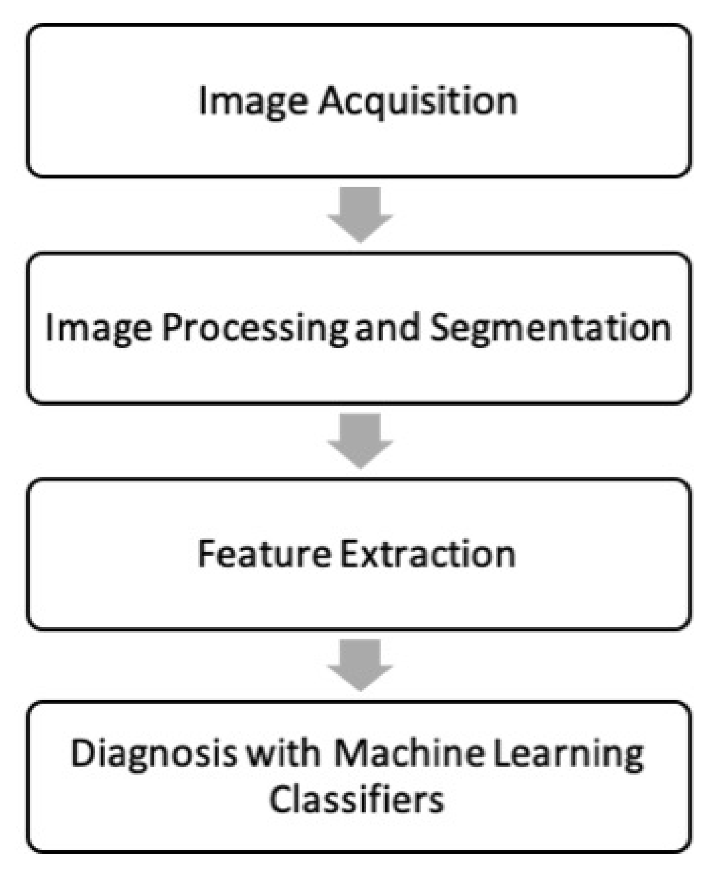
2. Materials and Methods
2.1. Image Acquisition
2.1.1. Patient Selection
Training and Testing Dataset
Validation Dataset
2.1.2. Imaging Protocol
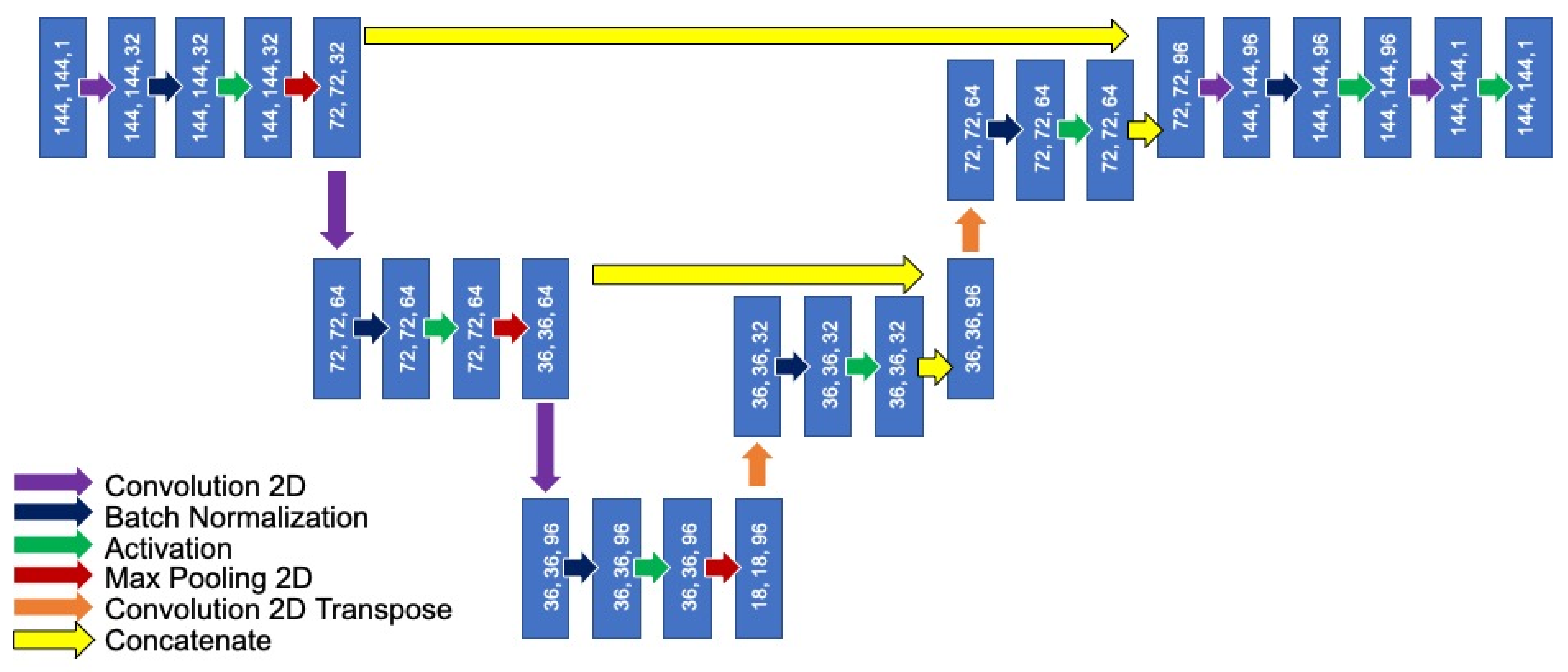
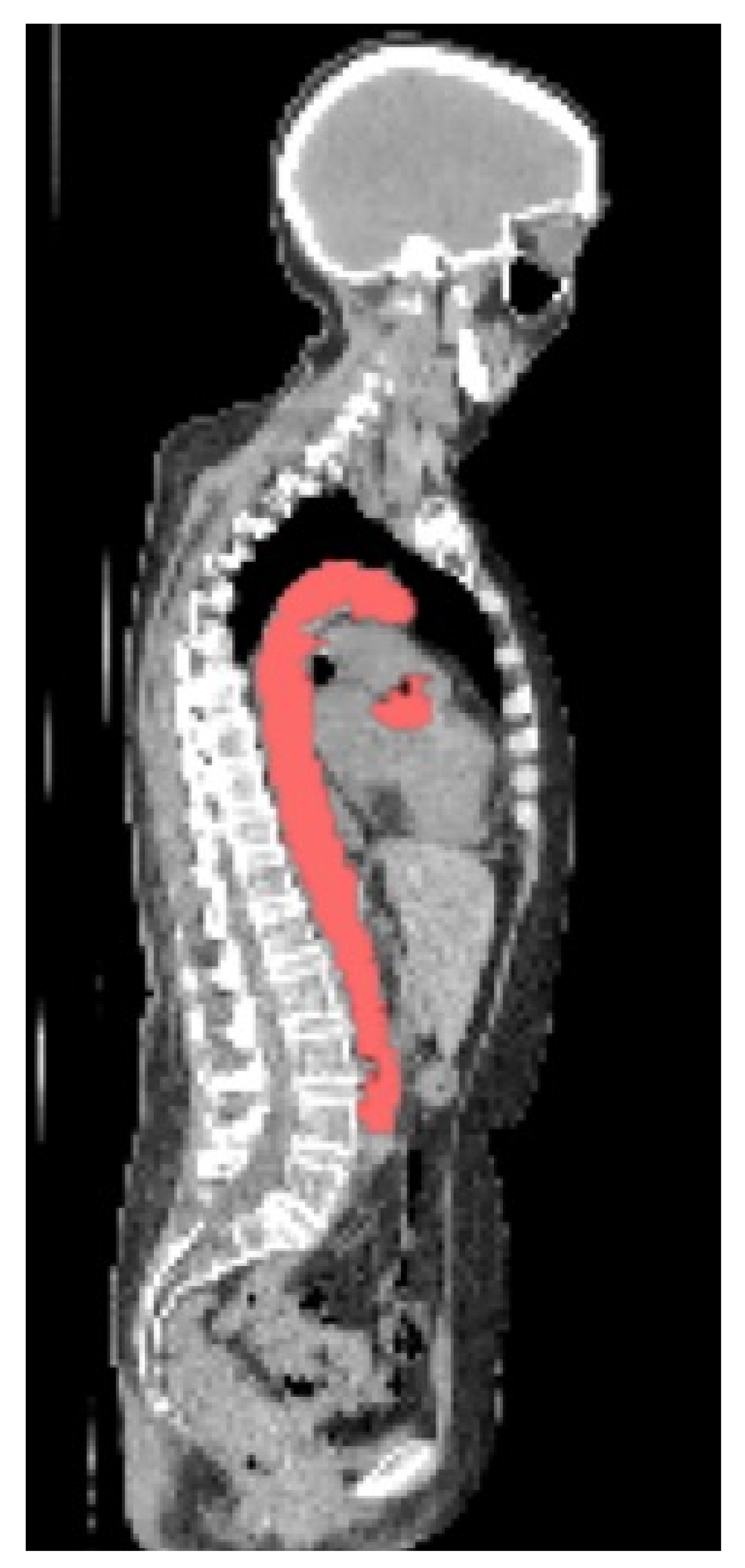
2.2. Image Processing and Segmentation
2.3. Feature Extraction
2.3.1. Qualitative Grading of Vessel Wall FDG Activity
2.3.2. Feature Extraction
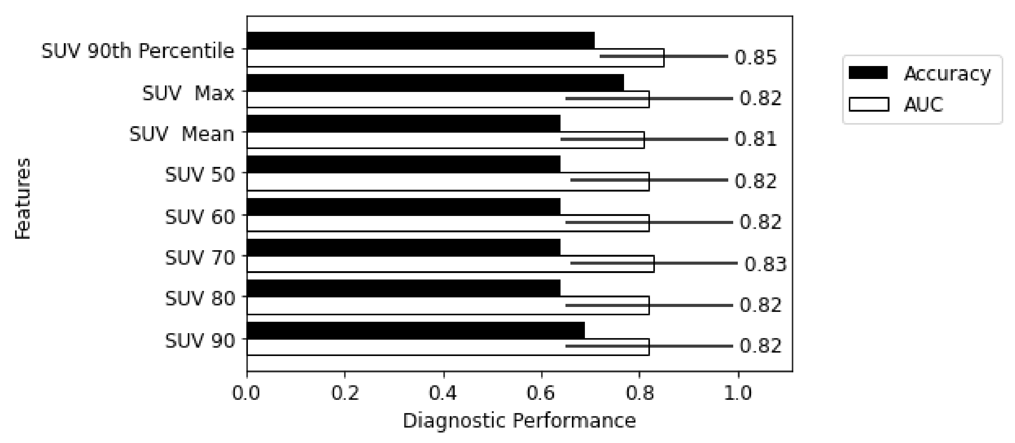
- SUV 90th Percentile—90% of the voxel’s SUV value fall below this number;
- SUV mean—the mean SUV value in the region of interest;
- SUV maximum—the maximum SUV value in the region of interest;
- SUV x (x = 50, 60, 70, 80, 90)—mean of the voxels that are equal or greater than x% of SUV maximum.
2.4. Diagnosis with Machine Learning Classifiers
2.4.1. Diagnostic Utility of Individual SUV Metrics and Radiomic Features
2.4.2. Forming Radiomic Fingerprints
2.4.3. Diagnostic Utility of Fingerprints
2.4.4. Statistical Analysis
2.5. The Influence of Variation in Method
2.5.1. Harmonization
2.5.2. Segmentation
2.5.3. Imaging Sources
3. Results
3.1. Image Acquisition—Patient Characteristics
3.2. Segmentation
3.3. Qualitative Grading of Vessel Wall FDG Activity
3.4. Diagnostic Utility of Individual SUV Metrics and Radiomic Features
3.5. Diagnostic Utility of Fingerprints
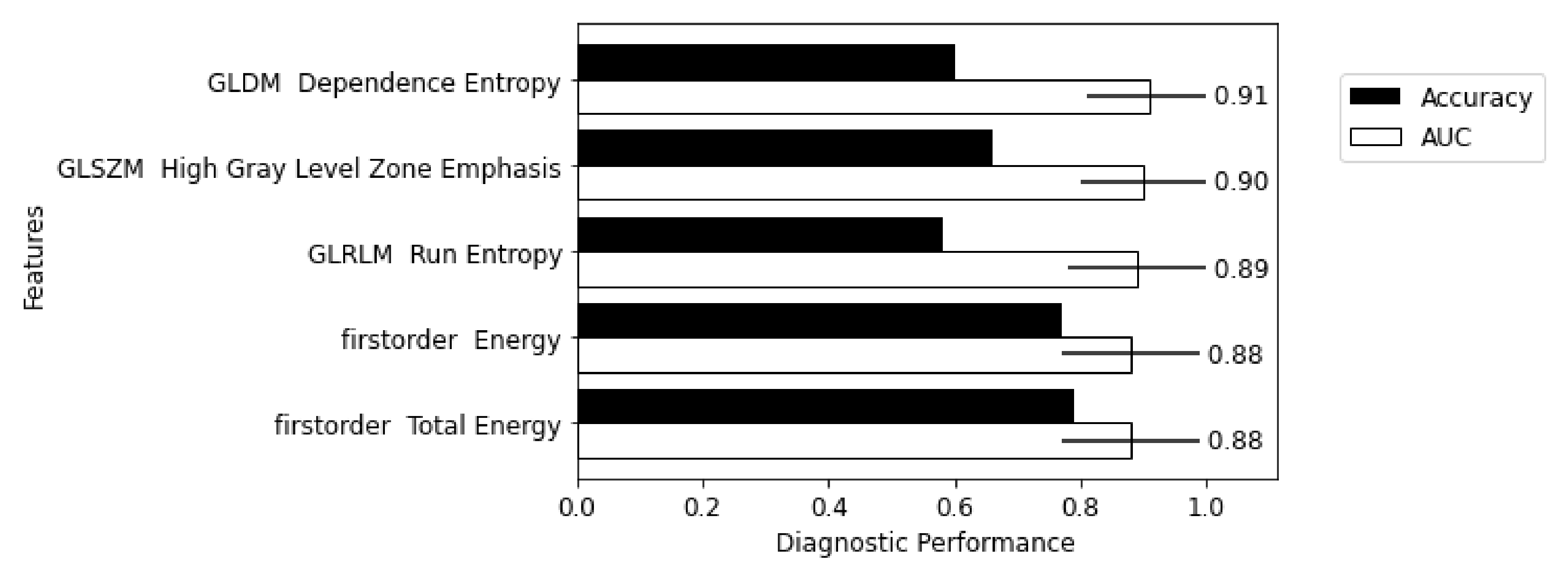
3.6. Comparison of Selected Features
3.7. Summary of Key Results
3.8. Influence of Variations in Method
4. Discussion
4.1. Segmentation Automation
4.2. Multi-Centre Transferability
4.3. Limitations
4.4. Harmonization and Standardization
5. Conclusions
Author Contributions
Funding
Institutional Review Board Statement
Informed Consent Statement
Data Availability Statement
Acknowledgments
Conflicts of Interest
Abbreviations
| SUV | Standardized Uptake Value |
| PCA | Principal Component Analysis |
| DSC | Dice Similarity Coefficient |
| AUC | Area Under the ROC Curve |
| ROC | Receiver Operating Characteristic |
| GCA | Giant Cell Arteritis |
| LVV | Large Vessel Vasculitis |
| FDG PET-CT | [18F]-Fluorodeoxyglucose Positron Emission Tomography—Computed |
| Tomography | |
| FDG | [18F]-Fluorodeoxyglucose |
| PET | Positron Emission Tomography |
| CT | Computed Tomography |
| GLDM | Gray-Level Dependence Matrix |
| GLCM | Gray-Level Co-Occurrence Matrix |
| GLRLM | Gray-Level Run Length Matrix |
| GLSZM | Gray-Level Size Zone Matrix |
| DLYD | Delayed Event Subtraction |
| TAK | Takayasu’s arteritis |
| CRP | C-Reactive Protein |
| ESR | Erythrocyte Sedimentation Rate |
| ML | Machine Learning |
| DL | Deep Learning |
| DICOM | Digital Imaging and Communications in Medicine |
| GPU | Graphics Processing Unit |
| PITA | PET Imaging of Giant Cell and Takayasu Arteritis |
| TARGET | Treatment According to Response in Giant Cell arTeritis |
| CNN | Convolutional Neural Network |
| EULAR | European Alliance of Associations for Rheumatology |
| EANM | European Association of Nuclear Medicine |
| SNMMI | Society of Nuclear Medicine and Molecular Imaging |
| ReLU | Rectified Linear Unit |
| AI | Artificial Intelligence |
| ROI | Region of Interest |
| IBSI | International Biomarker Standardisation Initiative |
| PACS | Picture Archiving and Communication |
| VPFX | Vue Point FX (3D time of flight) |
| SS-SIMUL | Single-scatter Simulation |
| BLOB-OS-TF | Spherically symmetric basis function ordered subset algorithm |
Appendix A. Imaging Protocol

| Scanner | Reconstruction | Scatter Correction | Randoms Correction | Matrix | Voxel Size |
|---|---|---|---|---|---|
| Gemini TF64 | BLOB-OS-TF | SS-SIMUL | DLYD | 144 | 4.00 × 4.00 × 4.00 |
| Discovery 710 | VPFX, QCFX, or VPHD | Model based | Singles | 192 | 3.65 × 3.65 × 3.27 |
| Discovery 690 | VPFX or VPFX | Model-based | Singles | 193 | 3.65 × 3.65 × 3.28 |
| Discovery MI DR | VPFX, QCFX, or VPHD | Model-based | SING | 256 | 2.73 × 2.73 × 3.27 |
| Discovery ST | OSEM | Convolution subtraction | DLYD | 128 | 4.69 × 4.69 × 3.27 |
| Discovery STE | OSEM | Convolution subtraction | SING | 128 | 5.47 × 5.47 × 3.27 |
| Biograph 6 True Point | OSEM2D 4i8s | Model-based | DLYD | 168 | 4.07 × 4.07 × 3.00 |
| Biograph 6 | OSEM2D 4i8s | Model-based | DLYD | 168 | 4.07 × 4.07 × 3.00 |
| Biograph 64 mCT | PSF + TOF 2i21s or OSEM3D 2i24s | Model-based | DLYD | 200 | 4.07 × 4.07 × 3.00 |
Appendix B. ML Parameters and Diagnostic Performance of Individual SUV metrics and Radiomic Features
| Feature | Params | ACC Training | AUC Training | AUC CI | ACC Test | AUC Test | AUC Test CI | ACC Val | AUC Val | AUC Val CI |
|---|---|---|---|---|---|---|---|---|---|---|
| original shape Elongation | (`C’, 3.8056144605552977), (`dual’, False), (`fit intercept’, True), (`intercept scaling’, 5), (`max iter’, 6310), (`penalty’, `l2’), (`random state’, 1), (`solver’, `liblinear’), (`tol’, 0.017923654340198922) | 0.500 | 0.585 | 0.455–0.716 | 0.500 | 0.617 | 0.239–0.994 | 0.500 | 0.614 | 0.497–0.732 |
| original firstorder 10 Percentile | (`C’, 2.8817940478533313), (`dual’, False), (`fit intercept’, True), (`intercept scaling’, 4), (`max iter’, 3403), (`penalty’, `l1’), (`random state’, 1), (`solver’, `liblinear’), (`tol’, 0.011518315256582621) | 0.676 | 0.825 | 0.554–1.000 | 0.558 | 0.700 | 0.387–1.000 | 0.637 | 0.784 | 0.690–0.879 |
| original firstorder 90 Percentile | (`C’, 1.774728175866115), (`dual’, False), (`fit intercept’, True), (`intercept scaling’, 5), (`max iter’, 7444), (`penalty’, `l1’), (`random state’, 1), (`solver’, `liblinear’), (`tol’, 0.08170692475524036) | 0.767 | 0.911 | 0.731–1.000 | 0.700 | 0.933 | 0.791–1.000 | 0.547 | 0.685 | 0.580–0.791 |
| original firstorder Energy | (`C’, 1.0), (`dual’, False), (`fit intercept’, True), (`intercept scaling’, 1), (`max iter’, 10,000), (`penalty’, `l1’), (`random state’, 1), (`solver’, `liblinear’), (`tol’, 0.02338512988384992) | 0.689 | 0.852 | 0.769–0.934 | 0.800 | 0.967 | 0.888–1.000 | 0.625 | 0.717 | 0.611–0.822 |
| original firstorder Entropy | (`C’, 3.898563938816272), (`dual’, False), (`fit intercept’, True), (`intercept scaling’, 5), (`max iter’, 1057), (`penalty’, `l2’), (`random state’, 1), (`solver’, `liblinear’), (`tol’, 0.09065383006063307) | 0.710 | 0.901 | 0.793–1.000 | 0.800 | 0.917 | 0.780–1.000 | 0.470 | 0.555 | 0.440–0.670 |
| original firstorder Interquartile Range | (`C’, 4.0), (`dual’, False), (`fit intercept’, True), (`intercept scaling’, 5), (`max iter’, 8442), (`penalty’, `l1’), (`random state’, 1), (`solver’, `liblinear’), (`tol’, 0.004402437057502587) | 0.712 | 0.834 | 0.771-0.896 | 0.658 | 0.850 | 0.652–1.000 | 0.448 | 0.531 | 0.415–0.647 |
| original firstorder Kurtosis | (`C’, 3.634835218565156), (`dual’, False), (`fit intercept’, True), (`intercept scaling’, 1), (`max iter’, 6758), (`penalty’, `l1’), (`random state’, 1), (`solver’, `liblinear’), (`tol’, 0.0013191637682750674) | 0.500 | 0.441 | 0.297–0.586 | 0.500 | 0.450 | 0.130–0.770 | 0.500 | 0.468 | 0.346–0.590 |
| original firstorder Maximum | (`C’, 3.5515515962056434), (`dual’, False), (`fit intercept’, True), (`intercept scaling’, 5), (`max iter’, 9296), (`penalty’, `l2’), (`random state’, 1), (`solver’, `liblinear’), (`tol’, 0.008690899693926512) | 0.606 | 0.764 | 0.456–1.000 | 0.800 | 0.967 | 0.888–1.000 | 0.537 | 0.508 | 0.384–0.632 |
| original firstorder Mean | (`C’, 3.9294940929254794), (`dual’, False), (`fit intercept’, True), (`intercept scaling’, 5), (`max iter’, 3769), (`penalty’, `l1’), (`random state’, 1), (`solver’, `liblinear’), (`tol’, 0.034137309056045194) | 0.767 | 0.890 | 0.668–1.000 | 0.800 | 0.883 | 0.647–1.000 | 0.598 | 0.724 | 0.620–0.828 |
| original firstorder MeanAbsoluteDeviation | (`C’, 4.0), (`dual’, False), (`fit intercept’, True), (`intercept scaling’, 1), (`max iter’, 10,000), (`penalty’, `l1’), (`random state’, 1), (`solver’, `liblinear’), (`tol’, 0.1) | 0.678 | 0.879 | 0.720–1.000 | 0.700 | 0.900 | 0.741–1.000 | 0.479 | 0.555 | 0.440–0.670 |
| original firstorder Median | (`C’, 3.9959470312560192), (`dual’, False), (`fit intercept’, True), (`intercept scaling’, 4), (`max iter’, 9514), (`penalty’, `l1’), (’`random state’, 1), (`solver’, `liblinear’), (`tol’, 0.003443979629449537) | 0.756 | 0.853 | 0.574–1.000 | 0.600 | 0.833 | 0.591–1.000 | 0.568 | 0.690 | 0.581–0.799 |
| original firstorder Minimum | (`C’, 3.676869725788), (`dual’, False), (`fit intercept’, True), (`intercept scaling’, 2), (`max iter’, 3060), (`penalty’, `l2’), (`random state’, 1), (`solver’, `liblinear’), (`tol’, 0.08958960709045656) | 0.500 | 0.432 | 0.147–0.717 | 0.500 | 0.417 | −0.025–0.858 | 0.500 | 0.743 | 0.635–0.851 |
| original firstorder Range | (`C’, 2.9625927896408317), (`dual’, False), (`fit intercept’, True), (`intercept scaling’, 5), (`max iter’, 5285), (`penalty’, `l1’), (`random state’, 1), (`solver’, `liblinear’), (`tol’, 0.04665607138780834) | 0.592 | 0.756 | 0.495–1.000 | 0.700 | 0.967 | 0.888–1.000 | 0.465 | 0.484 | 0.360–0.608 |
| original firstorder RobustMeanAbsoluteDeviation | (`C’, 4.0), (`dual’, False), (`fit intercept’, True), (`intercept scaling’, 2), (`max iter’, 6466), (`penalty’, `l1’), (`random state’, 1), (`solver’, `liblinear’), (`tol’, ) | 0.654 | 0.856 | 0.767–0.945 | 0.658 | 0.867 | 0.679–1.000 | 0.495 | 0.535 | 0.419–0.650 |
| original firstorder RootMeanSquared | (`C’, 3.9502570349836175), (`dual’, False), (`fit intercept’, True), (`intercept scaling’, 2), (`max iter’, 7402), (`penalty’, `l1’), (`random state’, 1), (`solver’, `liblinear’), (`tol’, 0.08258347919775297) | 0.767 | 0.900 | 0.710–1.000 | 0.600 | 0.883 | 0.647–1.000 | 0.585 | 0.718 | 0.614–0.822 |
| original firstorder Skewness | (`C’, 2.238056324193022), (`dual’, False), (`fit intercept’, True), (`intercept scaling’, 5), (`max iter’, 1545), (`penalty’, `l2’), (`random state’, 1), (`solver’, `liblinear’), (`tol’, 0.08427086764521606) | 0.489 | 0.568 | −0.004–1.000 | 0.500 | 0.850 | 0.613–1.000 | 0.500 | 0.613 | 0.495–0.731 |
| original firstorder Total Energy | (`C’, 1.292188045736975), (`dual’, False), (`fit intercept’, True), (`intercept scaling’, 1), (`max iter’, 9696), (`penalty’, `l1’), (`random state’, 1), (`solver’, `liblinear’), (`tol’, 0.00010802104590742912) | 0.689 | 0.852 | 0.769–0.934 | 0.800 | 0.967 | 0.888–1.000 | 0.662 | 0.717 | 0.611–0.822 |
| original firstorder Uniformity | (`C’, 3.39826558360898), (`dual’, False), (`fit intercept’, False), (`intercept scaling’, 5), (`max iter’, 7542), (`penalty’, `l2’), (`random state’, 1), (`solver’, `liblinear’), (`tol’, 0.07122003912935275) | 0.500 | 0.138 | 0.000–0.277 | 0.500 | 0.100 | −0.059–0.259 | 0.500 | 0.460 | 0.344–0.577 |
| original firstorder Variance | (`C’, 2.8454630117539024), (`dual’, False), (`fit intercept’, True), (`intercept scaling’, 2), (`max iter’, 5096), (`penalty’, `l1’), (`random state’, 1), (`solver’, `liblinear’), (`tol’, 0.007605136714617995) | 0.723 | 0.899 | 0.756–1.000 | 0.800 | 0.967 | 0.890–1.000 | 0.453 | 0.551 | 0.437–0.665 |
| original glcm Autocorrelation | (`C’, 4.0), (`dual’, False), (`fit intercept’, True), (`intercept scaling’, 5), (`max iter’, 10), (`penalty’, `l1’), (`random state’, 1), (`solver’, `liblinear’), (`tol’, ) | 0.798 | 0.894 | 0.786–1.000 | 0.700 | 0.950 | 0.839–1.000 | 0.469 | 0.604 | 0.493–0.716 |
| original glcm ClusterProminence | (`C’, 1.2014550932380232), (`dual’, False), (`fit intercept’, True), (`intercept scaling’, 5), (`max iter’, 1049), (`penalty’, `l1’), (`random state’, 1), (`solver’, `liblinear’), (`tol’, 0.02992266728475855) | 0.718 | 0.850 | 0.710-0.990 | 0.700 | 1.000 | nan–nan | 0.424 | 0.558 | 0.444–0.673 |
| original glcm ClusterShade | (`C’, 1.1562338815842363), (`dual’, False), (`fit intercept’, True), (`intercept scaling’, 4), (`max iter’, 10), (`penalty’, `l1’), (`random state’, 1), (`solver’, `liblinear’), (`tol’, 0.1) | 0.500 | 0.573 | 0.069-1.000 | 0.500 | 0.533 | 0.255–0.812 | 0.500 | 0.703 | 0.596–0.809 |
| original glcm ClusterTendency | (`C’, 3.3987720010803155), (`dual’, False), (`fit intercept’, True), (`intercept scaling’, 1), (`max iter’, 2281), (`penalty’, `l1’), (`random state’, 1), (`solver’, `liblinear’), (`tol’, 0.04646204360821551) | 0.743 | 0.894 | 0.753–1.000 | 0.800 | 0.933 | 0.813–1.000 | 0.451 | 0.579 | 0.465–0.692 |
| original glcm Contrast | (`C’, 2.794213383090132), (`dual’, False), (`fit intercept’, True), (`intercept scaling’, 4), (`max iter’, 7568), (`penalty’, `l2’), (`random state’, 1), (`solver’, `liblinear’), (`tol’, 0.09298732537139162) | 0.802 | 0.901 | 0.776–1.000 | 0.758 | 0.967 | 0.890–1.000 | 0.477 | 0.452 | 0.333–0.571 |
| original glcm Correlation | (`C’, 2.3265163816288474), (`dual’, False), (`fit intercept’, False), (`intercept scaling’, 3), (`max iter’, 7116), (`penalty’, `l2’), (`random state’, 1), (`solver’, `liblinear’), (`tol’, 0.0188936121493807) | 0.500 | 0.423 | 0.244–0.603 | 0.500 | 0.367 | 0.068–0.665 | 0.500 | 0.768 | 0.658–0.877 |
| original glcm Difference Average | (`C’, 3.765281617061703), (`dual’, False), (`fit intercept’, True), (`intercept scaling’, 5), (`max iter’, 3203), (`penalty’, `l2’), (`random state’, 1), (`solver’, `liblinear’), (`tol’, 0.04678697115468039) | 0.762 | 0.896 | 0.769–1.000 | 0.800 | 0.900 | 0.742–1.000 | 0.502 | 0.436 | 0.316–0.556 |
| original glcm Difference Entropy | (`C’, 2.5454905419682645), (`dual’, False), (`fit intercept’, True), (`intercept scaling’, 4), (`max iter’, 7232), (`penalty’, `l1’), (`random state’, 1), (`solver’, `liblinear’), (`tol’, 0.013588632723062564) | 0.748 | 0.896 | 0.769-1.000 | 0.800 | 0.933 | 0.814–1.000 | 0.518 | 0.436 | 0.316–0.555 |
| original glcm Difference Variance | (`C’, 1.0), (`dual’, False), (`fit intercept’, True), (`intercept scaling’, 4), (`max iter’, 10), (`penalty’, `l1’), (`random state’, 1), (`solver’, `liblinear’), (`tol’, 0.1) | 0.774 | 0.901 | 0.771-1.000 | 0.800 | 0.967 | 0.890–1.000 | 0.487 | 0.462 | 0.343–0.580 |
| original glcm Id | (`C’, 2.876700911377709), (`dual’, False), (`fit intercept’, True), (`intercept scaling’, 3), (`max iter’, 5860), (`penalty’, `l1’), (`random state’, 1), (`solver’, `liblinear’), (`tol’, 0.021468961778094153) | 0.628 | 0.862 | 0.741–0.982 | 0.600 | 0.900 | 0.742–1.000 | 0.475 | 0.401 | 0.282–0.521 |
| original glcm Idm | (`C’, 3.5521886140988324), (`dual’, False), (`fit intercept’, True), (`intercept scaling’, 1), (`max iter’, 10), (`penalty’, `l1’), (`random state’, 1), (`solver’, `liblinear’), (`tol’, ) | 0.639 | 0.862 | 0.741–0.982 | 0.600 | 0.900 | 0.742–1.000 | 0.475 | 0.394 | 0.275–0.513 |
| original glcm Idmn | (`C’, 2.5729756259638257), (`dual’, False), (`fit intercept’, False), (`intercept scaling’, 4), (`max iter’, 6648), (`penalty’, `l1’), (`random state’, 1), (`solver’, `liblinear’), (`tol’, 0.0722906499673705) | 0.500 | 0.369 | 0.187–0.551 | 0.500 | 0.500 | 0.222–0.778 | 0.500 | 0.561 | 0.437–0.685 |
| original glcm Idn | (`C’, 1.5612853647891844), (`dual’, False), (`fit intercept’, True), (`intercept scaling’, 4), (`max iter’, 8056), (`penalty’, `l2’), (`random state’, 1), (`solver’, `liblinear’), (`tol’, 0.031534182504912224) | 0.500 | 0.390 | 0.205–0.575 | 0.500 | 0.517 | 0.236–0.798 | 0.500 | 0.586 | 0.464–0.709 |
| original glcm Imc1 | (`C’, 3.9438796427354554), (`dual’, False), (`fit intercept’, False), (`intercept scaling’, 3), (`max iter’, 9320), (`penalty’, `l1’), (`random state’, 1), (`solver’, `liblinear’), (`tol’, 0.09874439787032405) | 0.500 | 0.440 | 0.182–0.698 | 0.500 | 0.333 | 0.067–0.600 | 0.500 | 0.796 | 0.693–0.900 |
| original glcm Imc2 | (`C’, 2.543363070723238), (`dual’, False), (`fit intercept’, True), (`intercept scaling’, 5), (`max iter’, 2274), (`penalty’, `l1’), (`random state’, 1), (`solver’, `liblinear’), (`tol’, 0.00834386841277177) | 0.500 | 0.500 | nan–nan | 0.500 | 0.517 | 0.208–0.825 | 0.500 | 0.783 | 0.684–0.882 |
| original glcm Inverse Variance | (`C’, 3.2073129630396777), (`dual’, False), (`fit intercept’, True), (`intercept scaling’, 4), (`max iter’, 6658), (`penalty’, `l1’), (`random state’, 1), (`solver’, `liblinear’), (`tol’, 0.0074434857032721225) | 0.628 | 0.862 | 0.741–0.982 | 0.700 | 0.900 | 0.742–1.000 | 0.490 | 0.398 | 0.278–0.518 |
| original glcm JointAverage | (`C’, 2.884522523620075), (`dual’, False), (`fit intercept’, True), (`intercept scaling’, 3), (`max iter’, 10), (`penalty’, `l2’), (`random state’, 1), (`solver’, `liblinear’), (`tol’, 0.018889093800706636) | 0.714 | 0.894 | 0.802–0.987 | 0.700 | 0.900 | 0.742–1.000 | 0.501 | 0.591 | 0.478–0.703 |
| original glcm JointEnergy | (`C’, 1.199944589432079), (`dual’, False), (`fit intercept’, True), (`intercept scaling’, 3), (`max iter’, 45), (`penalty’, `l2’), (`random state’, 1), (`solver’, `liblinear’), (`tol’, 0.09140428650296156) | 0.500 | 0.851 | 0.767–0.934 | 0.500 | 0.933 | 0.814–1.000 | 0.500 | 0.478 | 0.361–0.594 |
| original glcm JointAverage | (`C’, 2.884522523620075), (`dual’, False), (`fit intercept’, True), (`intercept scaling’, 3), (`max iter’, 10), (`penalty’, `l2’), (`random state’, 1), (`solver’, `liblinear’), (`tol’, 0.018889093800706636) | 0.714 | 0.894 | 0.802–0.987 | 0.700 | 0.900 | 0.742–1.000 | 0.501 | 0.591 | 0.478–0.703 |
| original glcm Joint Energy | (`C’, 1.199944589432079), (`dual’, False), (`fit intercept’, True), (`intercept scaling’, 3), (`max iter’, 45), (`penalty’, `l2’), (`random state’, 1), (`solver’, `liblinear’), (`tol’, 0.09140428650296156) | 0.500 | 0.851 | 0.767-0.934 | 0.500 | 0.933 | 0.814–1.000 | 0.500 | 0.478 | 0.361–0.594 |
| original glcm Joint Entropy | (`C’, 2.8485013507009964), (`dual’, False), (`fit intercept’, True), (`intercept scaling’, 3), (`max iter’, 1666), (`penalty’, `l1’), (`random state’, 1), (`solver’, `liblinear’), (`tol’, 0.0003388234219221265) | 0.710 | 0.883 | 0.758-1.000 | 0.800 | 0.933 | 0.814–1.000 | 0.462 | 0.500 | 0.383–0.616 |
| original glcm MCC | (`C’, 3.7544969295345636), (`dual’, False), (`fit intercept’, True), (`intercept scaling’, 4), (`max iter’, 7337), (`penalty’, `l1’), (`random state’, 1), (`solver’, `liblinear’), (`tol’, 0.02150123778633736) | 0.500 | 0.454 | 0.342–0.565 | 0.500 | 0.533 | 0.213–0.854 | 0.500 | 0.593 | 0.470–0.717 |
| original glcm Maximum Probability | (`C’, 3.749171778156825), (`dual’, False), (`fit intercept’, False), (`intercept scaling’, 4), (`max iter’, 9343), (`penalty’, `l2’), (`random state’, 1), (`solver’, `liblinear’), (`tol’, 0.039031034588965174) | 0.500 | 0.156 | 0.076–0.235 | 0.500 | 0.100 | −0.058–0.258 | 0.500 | 0.558 | 0.441–0.674 |
| original glcm Sum Average | (`C’, 1.2810898302218976), (`dual’, False), (`fit intercept’, True), (`intercept scaling’, 4), (`max iter’, 3097), (`penalty’, `l1’), (`random state’, 1), (`solver’, `liblinear’), (`tol’, 0.07161938424684904) | 0.714 | 0.894 | 0.802–0.987 | 0.700 | 0.900 | 0.742–1.000 | 0.501 | 0.591 | 0.478–0.703 |
| original glcm Sum Entropy | (`C’, 4.0), (`dual’, False), (`fit intercept’, True), (`intercept scaling’, 5), (`max iter’, 8498), (`penalty’, `l1’), (`random state’, 1), (`solver’, `liblinear’), (`tol’, ) | 0.705 | 0.901 | 0.793–1.000 | 0.800 | 0.900 | 0.741–1.000 | 0.452 | 0.586 | 0.473–0.699 |
| original glcm Sum Squares | (`C’, 1.305357350462431), (`dual’, False), (`fit intercept’, True), (`intercept scaling’, 1), (`max iter’, 339), (`penalty’, `l1’), (`random state’, 1), (`solver’, `liblinear’), (`tol’, 0.0006889623638318466) | 0.755 | 0.895 | 0.754–1.000 | 0.800 | 0.967 | 0.890–1.000 | 0.452 | 0.554 | 0.440–0.668 |
| original gldm Dependence Entropy | (`C’, 3.7717457451609153), (`dual’, False), (`fit intercept’, True), (`intercept scaling’, 4), (`max iter’, 14), (`penalty’, `l1’), (`random state’, 1), (`solver’, `liblinear’), (`tol’, 0.009597244103991846) | 0.539 | 0.807 | 0.605–1.000 | 0.500 | 0.917 | 0.743–1.000 | 0.500 | 0.812 | 0.729–0.896 |
| original gldm Dependence Non-Uniformity | (`C’, 4.0), (`dual’, False), (`fit intercept’, True), (`intercept scaling’, 5), (`max iter’, 10), (`penalty’, `l2’), (`random state’, 1), (`solver’, `liblinear’), (`tol’, ) | 0.598 | 0.696 | 0.359–1.000 | 0.800 | 0.933 | 0.814–1.000 | 0.468 | 0.502 | 0.381–0.623 |
| original gldm Dependence Non-Uniformity Normalized | (`C’, 3.9397386998320325), (`dual’, False), (`fit intercept’, True), (`intercept scaling’, 1), (`max iter’, 5358), (`penalty’, `l2’), (`random state’, 1), (`solver’, `liblinear’), (`tol’, 0.058125565483952035) | 0.500 | 0.805 | 0.647–0.963 | 0.500 | 0.883 | 0.718–1.000 | 0.500 | 0.370 | 0.253–0.486 |
| original gldm Dependence Variance | (`C’, 3.908072013043827), (`dual’, False), (`fit intercept’, True), (`intercept scaling’, 4), (`max iter’, 1551), (`penalty’, `l1’), (`random state’, 1), (`solver’, `liblinear’), (`tol’, 0.026849446139380312) | 0.639 | 0.795 | 0.620–0.970 | 0.658 | 0.850 | 0.660–1.000 | 0.443 | 0.303 | 0.191–0.415 |
| original gldm Gray Level Non-Uniformity | (`C’, 3.1826657805845513), (`dual’, False), (`fit intercept’, True), (`intercept scaling’, 5), (`max iter’, 9909), (`penalty’, `l2’), (`random state’, 1), (`solver’, `liblinear’), (`tol’, 0.0008888365484206898) | 0.676 | 0.779 | 0.447–1.000 | 0.558 | 0.600 | 0.288–0.912 | 0.474 | 0.468 | 0.344–0.593 |
| original gldm Gray Level Variance | (`C’, 1.8552309464866807), (`dual’, False), (`fit intercept’, True), (`intercept scaling’, 1), (`max iter’, 4836), (`penalty’, `l2’), (`random state’, 1), (`solver’, `liblinear’), (`tol’, 0.0019131772861938168) | 0.730 | 0.899 | 0.756–1.000 | 0.800 | 0.967 | 0.890–1.000 | 0.468 | 0.551 | 0.437–0.666 |
| original gldm High Gray Level Emphasis | (`C’, 4.0), (`dual’, False), (`fit intercept’, True), (`intercept scaling’, 5), (`max iter’, 10000), (`penalty’, `l1’), (`random state’, 1), (`solver’, `liblinear’), (`tol’, 0.04047765497803527) | 0.823 | 0.906 | 0.812–0.999 | 0.700 | 0.967 | 0.888–1.000 | 0.484 | 0.602 | 0.490–0.713 |
| original gldm Large Dependence Emphasis | (`C’, 1.0588224326821771), (`dual’, False), (`fit intercept’, True), (`intercept scaling’, 2), (`max iter’, 9519), (`penalty’, `l2’), (`random state’, 1), (`solver’, `liblinear’), (`tol’, 0.047865873089018005) | 0.673 | 0.828 | 0.648–1.000 | 0.700 | 0.883 | 0.718–1.000 | 0.459 | 0.351 | 0.234–0.468 |
| original gldm Large Dependence High Gray Level Emphasis | (`C’, 3.1168548949137724), (`dual’, False), (`fit intercept’, False), (`intercept scaling’, 2), (`max iter’, 1217), (`penalty’, `l2’), (`random state’, 1), (`solver’, `liblinear’), (`tol’, 0.0838087387972799) | 0.500 | 0.557 | 0.111–1.000 | 0.500 | 0.467 | 0.123–0.810 | 0.500 | 0.753 | 0.640–0.865 |
| original gldm LowGray LevelEmphasis | (`C’, 2.8291349845222524), (`dual’, False), (`fit intercept’, True), (`intercept scaling’, 5), (`max iter’, 7077), (`penalty’, `l1’), (`random state’, 1), (`solver’, `liblinear’), (`tol’, 0.03740604869362484) | 0.500 | 0.500 | nan–nan | 0.500 | 0.500 | nan–nan | 0.500 | 0.500 | nan–nan |
| original gldm SmallDependenceEmphasis | (`C’, 3.9838817245979876), (`dual’, False), (`fit intercept’, True), (`intercept scaling’, 5), (`max iter’, 1542), (`penalty’, `l1’), (`random state’, 1), (`solver’, `liblinear’), (`tol’, 0.0008766419147272496) | 0.710 | 0.867 | 0.699–1.000 | 0.800 | 0.900 | 0.742–1.000 | 0.534 | 0.407 | 0.287–0.527 |
| original gldm Small Dependence High Gray Level Emphasis | (`C’, 4.0), (`dual’, False), (`fit intercept’, True), (`intercept scaling’, 2), (`max iter’, 2813), (`penalty’, `l1’), (`random state’, 1), (`solver’, `liblinear’), (`tol’, 0.05195113774499899) | 0.773 | 0.929 | 0.832–1.000 | 0.800 | 0.983 | 0.937–1.000 | 0.491 | 0.525 | 0.409–0.641 |
| original gldm Small Dependence Low Gray Level Emphasis | (`C’, 2.030332175989515), (`dual’, False), (`fit intercept’, True), (`intercept scaling’, 5), (`max iter’, 5234), (`penalty’, `l2’), (`random state’, 1), (`solver’, `liblinear’), (`tol’, 0.006906386148325776) | 0.500 | 0.381 | −0.008–0.770 | 0.500 | 0.333 | 0.034–0.633 | 0.500 | 0.282 | 0.176–0.387 |
| original glrlm Gray Level Non-Uniformity | (`C’, 4.0), (`dual’, False), (`fit intercept’, True), (`intercept scaling’, 3), (`max iter’, 10), (`penalty’, `l1’), (`random state’, 1), (`solver’, `liblinear’), (`tol’, 0.1) | 0.662 | 0.751 | 0.421–1.000 | 0.558 | 0.550 | 0.211–0.889 | 0.467 | 0.486 | 0.361–0.612 |
| original glrlm Gray Level Non-Uniformity Normalized | (`C’, 3.8458368662008255), (`dual’, False), (`fit intercept’, False), (`intercept scaling’, 3), (`max iter’, 3365), (`penalty’, `l2’), (`random state’, 1), (`solver’, `liblinear’), (`tol’, 0.014454416417432375) | 0.500 | 0.133 | 0.011–0.255 | 0.500 | 0.117 | −0.050–0.283 | 0.500 | 0.457 | 0.341–0.573 |
| original glrlm Gray Level Variance | (`C’, 1.6722052556540499), (`dual’, False), (`fit intercept’, True), (`intercept scaling’, 5), (`max iter’, 10), (`penalty’, `l1’), (`random state’, 1), (`solver’, `liblinear’), (`tol’, 0.1) | 0.723 | 0.905 | 0.764–1.000 | 0.700 | 0.967 | 0.890–1.000 | 0.432 | 0.554 | 0.440–0.668 |
| original glrlm High Gray Level RunEmphasis | (`C’, 4.0), (`dual’, False), (`fit intercept’, True), (`intercept scaling’, 5), (`max iter’, 10000), (`penalty’, `l1’), (`random state’, 1), (`solver’, `liblinear’), (`tol’, 0.05118583169143218) | 0.812 | 0.906 | 0.812–0.999 | 0.700 | 0.967 | 0.888–1.000 | 0.476 | 0.606 | 0.494–0.717 |
| original glrlm Long Run Emphasis | (`C’, 3.833856019580739), (`dual’, False), (`fit intercept’, True), (`intercept scaling’, 3), (`max iter’, 1631), (`penalty’, `l1’), (`random state’, 1), (`solver’, `liblinear’), (`tol’, 0.03501141624853724) | 0.639 | 0.844 | 0.675–1.000 | 0.600 | 0.883 | 0.718-1.000 | 0.467 | 0.362 | 0.244–0.480 |
| original glrlm Long Run High Gray Level Emphasis | (`C’, 4.0), (`dual’, False), (`fit intercept’, True), (`intercept scaling’, 3), (`max iter’, 4806), (`penalty’, `l1’), (`random state’, 1), (`solver’, `liblinear’), (`tol’, 0.018730143457553885) | 0.753 | 0.884 | 0.740–1.000 | 0.700 | 0.967 | 0.890–1.000 | 0.500 | 0.654 | 0.545–0.762 |
| original glrlm LongRunLowGray LevelEmphasis | (`C’, 2.6289220027281743), (`dual’, False), (`fit intercept’, True), (`intercept scaling’, 1), (`max iter’, 7056), (`penalty’, `l2’), (`random state’, 1), (`solver’, `liblinear’), (`tol’, 0.09003136591880305) | 0.500 | 0.861 | 0.738–0.984 | 0.500 | 0.867 | 0.680–1.000 | 0.500 | 0.657 | 0.547–0.767 |
| original glrlm Low Gray Level Run Emphasis | (`C’, 2.2376337828274573), (`dual’, False), (`fit intercept’, False), (`intercept scaling’, 4), (`max iter’, 7747), (`penalty’, `l2’), (`random state’, 1), (`solver’, `liblinear’), (`tol’, 0.07030672418295693) | 0.500 | 0.157 | −0.012–0.325 | 0.500 | 0.133 | −0.054–0.320 | 0.500 | 0.310 | 0.204-0.417 |
| original glrlm RunEntropy | (`C’, 3.3114257300096157), (`dual’, False), (`fit intercept’, True), (`intercept scaling’, 5), (`max iter’, 121), (`penalty’, `l2’), (`random state’, 1), (`solver’, `liblinear’), (`tol’, 0.0194354228138649) | 0.690 | 0.889 | 0.748–1.000 | 0.700 | 0.917 | 0.780–1.000 | 0.464 | 0.606 | 0.493–0.718 |
| original glrlm Run Length Non-Uniformity | (`C’, 1.4366614662702664), (`dual’, False), (`fit intercept’, False), (`intercept scaling’, 1), (`max iter’, 2709), (`penalty’, `l2’), (`random state’, 1), (`solver’, `liblinear’), (`tol’, 0.03928484749498973) | 0.500 | 0.611 | 0.104–1.000 | 0.500 | 0.967 | 0.890–1.000 | 0.500 | 0.555 | 0.434–0.676 |
| original glrlm Run Length Non-Uniformity Normalized | (`C’, 2.6720853872765495), (`dual’, False), (`fit intercept’, False), (`intercept scaling’, 3), (`max iter’, 3774), (`penalty’, `l2’), (`random state’, 1), (`solver’, `liblinear’), (`tol’, 0.07427424237615005) | 0.500 | 0.839 | 0.684–0.993 | 0.500 | 0.900 | 0.742–1.000 | 0.500 | 0.378 | 0.259–0.496 |
| original glrlm RunPercentage | (`C’, 2.6023123244300974), (`dual’, False), (`fit intercept’, True), (`intercept scaling’, 2), (`max iter’, 291), (`penalty’, `l1’), (`random state’, 1), (`solver’, `liblinear’), (`tol’, 0.049781425459564835) | 0.500 | 0.839 | 0.684–0.993 | 0.500 | 0.883 | 0.718–1.000 | 0.500 | 0.370 | 0.251–0.488 |
| original glrlm RunVariance | (`C’, 3.61481821528191), (`dual’, False), (`fit intercept’, True), (`intercept scaling’, 1), (`max iter’, 10), (`penalty’, `l1’), (`random state’, 1), (`solver’, `liblinear’), (`tol’, ) | 0.564 | 0.834 | 0.651–1.000 | 0.600 | 0.867 | 0.689–1.000 | 0.467 | 0.347 | 0.231–0.464 |
| original glrlm ShortRunEmphasis | (`C’, 2.732198485448542), (`dual’, False), (`fit intercept’, True), (`intercept scaling’, 2), (`max iter’, 974), (`penalty’, `l2’), (`random state’, 1), (`solver’, `liblinear’), (`tol’, 0.01734471841788434) | 0.500 | 0.839 | 0.684–0.993 | 0.500 | 0.900 | 0.742–1.000 | 0.500 | 0.377 | 0.258–0.495 |
| original glrlm Short Run High Gray Level Emphasis | (`C’, 3.9351523410188607), (`dual’, False), (`fit intercept’, True), (`intercept scaling’, 3), (`max iter’, 2339), (`penalty’, `l1’), (`random state’, 1), (`solver’, `liblinear’), (`tol’, 0.06576459057456105) | 0.787 | 0.906 | 0.812-0.999 | 0.800 | 0.967 | 0.888-1.000 | 0.476 | 0.594 | 0.482-0.706 |
| original glrlm Short Run Low Gray Level Emphasis | (`C’, 3.4237606654811574), (`dual’, False), (`fit intercept’, True), (`intercept scaling’, 2), (`max iter’, 1707), (`penalty’, `l2’), (`random state’, 1), (`solver’, `liblinear’), (`tol’, 0.06073466346615761) | 0.500 | 0.833 | 0.660-1.000 | 0.500 | 0.867 | 0.680-1.000 | 0.500 | 0.695 | 0.590–0.801 |
| original glszm Gray Level Non-Uniformity | (`C’, 3.8458029875767066), (`dual’, False), (`fit intercept’, True), (`intercept scaling’, 1), (`max iter’, 2474), (`penalty’, `l2’), (`random state’, 1), (`solver’, `liblinear’), (`tol’, 0.04148253163117249) | 0.500 | 0.635 | 0.355–0.915 | 0.500 | 0.850 | 0.661–1.000 | 0.500 | 0.428 | 0.306–0.549 |
| original glszm Gray Level Non-Uniformity Normalized | (`C’, 3.600665976879018), (`dual’, False), (`fit intercept’, True), (`intercept scaling’, 3), (`max iter’, 1678), (`penalty’, `l2’), (`random state’, 1), (`solver’, `liblinear’), (`tol’, 0.05947499893500212) | 0.500 | 0.894 | 0.770–1.000 | 0.500 | 0.983 | 0.937–1.000 | 0.500 | 0.573 | 0.459–0.687 |
| original glszm Gray Level Variance | (`C’, 2.901196262126115), (`dual’, False), (`fit intercept’, True), (`intercept scaling’, 1), (`max iter’, 10), (`penalty’, `l1’), (`random state’, 1), (`solver’, `liblinear’), (`tol’, 0.03774426454693599) | 0.749 | 0.860 | 0.721–0.999 | 0.800 | 1.000 | nan–nan | 0.453 | 0.575 | 0.461–0.688 |
| original glszm High Gray Level Zone Emphasis | (`C’, 3.478204583582132), (`dual’, False), (`fit intercept’, True), (`intercept scaling’, 2), (`max iter’, 1616), (`penalty’, `l1’), (`random state’, 1), (`solver’, `liblinear’), (`tol’, 0.09703590654231291) | 0.762 | 0.905 | 0.829–0.981 | 0.800 | 0.983 | 0.937–1.000 | 0.453 | 0.601 | 0.489–0.712 |
| original glszm Large Area Emphasis | (`C’, 1.6046715254557193), (`dual’, False), (`fit intercept’, True), (`intercept scaling’, 5), (`max iter’, 6822), (`penalty’, `l1’), (`random state’, 1), (`solver’, `liblinear’), (`tol’, 0.07800900631220041) | 0.648 | 0.851 | 0.652–1.000 | 0.700 | 0.867 | 0.689–1.000 | 0.490 | 0.378 | 0.260–0.496 |
| original glszm Large Area High Gray Level Emphasis | (`C’, 1.8487035352590049), (`dual’, False), (`fit intercept’, True), (`intercept scaling’, 2), (`max iter’, 1179), (`penalty’, `l1’), (`random state’, 1), (`solver’, `liblinear’), (`tol’, 0.05701958294758005) | 0.553 | 0.812 | 0.550–1.000 | 0.700 | 0.850 | 0.653–1.000 | 0.483 | 0.357 | 0.236–0.478 |
| original glszm Large Area Low Gray Level Emphasis | (`C’, 2.3369045710562144), (`dual’, False), (`fit intercept’, True), (`intercept scaling’, 2), (`max iter’, 7065), (`penalty’, `l2’), (`random state’, 1), (`solver’, `liblinear’), (`tol’, 0.08366919609286493) | 0.673 | 0.853 | 0.674–1.000 | 0.558 | 0.867 | 0.690–1.000 | 0.467 | 0.425 | 0.307–0.543 |
| original glszm Low Gray Level Zone Emphasis | (`C’, 2.0825064626116987), (`dual’, False), (`fit intercept’, True), (`intercept scaling’, 5), (`max iter’, 469), (`penalty’, `l1’), (`random state’, 1), (`solver’, `liblinear’), (`tol’, 0.05187162786375553) | 0.500 | 0.500 | nan–nan | 0.500 | 0.500 | nan–nan | 0.500 | 0.500 | nan–nan |
| original glszm Size Zone Non-Uniformity | (`C’, 3.4968658660509293), (`dual’, False), (`fit intercept’, True), (`intercept scaling’, 5), (`max iter’, 5119), (`penalty’, `l1’), (`random state’, 1), (`solver’, `liblinear’), (`tol’, 0.09985912291392018) | 0.705 | 0.849 | 0.793–0.905 | 0.800 | 0.967 | 0.890–1.000 | 0.475 | 0.489 | 0.370–0.609 |
| original glszm Size Zone Non-Uniformity Normalized | (`C’, 4.0), (`dual’, False), (`fit intercept’, True), (`intercept scaling’, 3), (`max iter’, 1220), (`penalty’, `l1’), (`random state’, 1), (`solver’, `liblinear’), (`tol’, 0.0010447413452487947) | 0.653 | 0.907 | 0.773–1.000 | 0.700 | 0.967 | 0.888–1.000 | 0.496 | 0.429 | 0.309–0.549 |
| original glszm Small Area Emphasis | (`C’, 3.6221746139345705), (`dual’, False), (`fit intercept’, True), (`intercept scaling’, 3), (`max iter’, 813), (`penalty’, `l1’), (`random state’, 1), (`solver’, `liblinear’), (`tol’, 0.004130953766069213) | 0.614 | 0.896 | 0.738–1.000 | 0.600 | 0.967 | 0.888–1.000 | 0.520 | 0.427 | 0.308–0.547 |
| original glszm Small Area High Gray Level Emphasis | (`C’, 2.6240187371586012), (`dual’, False), (`fit intercept’, True), (`intercept scaling’, 2), (`max iter’, 3622), (`penalty’, `l1’), (`random state’, 1), (`solver’, `liblinear’), (`tol’, 0.08556868775028845) | 0.762 | 0.900 | 0.795–1.000 | 0.800 | 1.000 | nan–nan | 0.478 | 0.553 | 0.439–0.667 |
| original glszm Small Area Low Gray Level Emphasis | (`C’, 1.7064389360641852), (`dual’, False), (`fit intercept’, True), (`intercept scaling’, 1), (`max iter’, 9885), (`penalty’, `l2’), (`random state’, 1), (`solver’, `liblinear’), (`tol’, 0.07794842268900995) | 0.500 | 0.837 | 0.733–0.941 | 0.500 | 0.867 | 0.688–1.000 | 0.500 | 0.590 | 0.478–0.702 |
| original glszm Zone Entropy | (`C’, 2.8550691194553095), (`dual’, False), (`fit intercept’, True), (`intercept scaling’, 2), (`max iter’, 3433), (`penalty’, `l1’), (`random state’, 1), (`solver’, `liblinear’), (`tol’, 0.06520910207277585) | 0.500 | 0.708 | 0.456–0.960 | 0.500 | 0.883 | 0.678–1.000 | 0.500 | 0.772 | 0.680–0.864 |
| original glszm Zone Percentage | (`C’, 4.0), (`dual’, False), (`fit intercept’, True), (`intercept scaling’, 2), (`max iter’, 956), (`penalty’, `l1’), (`random state’, 1), (`solver’, `liblinear’), (`tol’, ) | 0.710 | 0.874 | 0.698-1.000 | 0.800 | 0.900 | 0.742–1.000 | 0.534 | 0.409 | 0.290–0.529 |
| original glszm Zone Variance | (`C’, 2.2299373803328835), (`dual’, False), (`fit intercept’, True), (`intercept scaling’, 3), (`max iter’, 8739), (`penalty’, `l2’), (`random state’, 1), (`solver’, `liblinear’), (`tol’, 0.05624148106047668) | 0.623 | 0.850 | 0.654–1.000 | 0.700 | 0.867 | 0.689–1.000 | 0.490 | 0.375 | 0.258–0.493 |
| original shape Flatness | (`C’, 3.26351153620514), (`dual’, False), (`fit intercept’, True), (`intercept scaling’, 2), (`max iter’, 4285), (`penalty’, `l1’), (`random state’, 1), (`solver’, `liblinear’), (`tol’, 0.07375765313681576) | 0.500 | 0.500 | nan–nan | 0.500 | 0.500 | nan–nan | 0.500 | 0.500 | nan–nan |
| original shape Least Axis Length | (`C’, 2.226917940773356), (`dual’, False), (`fit intercept’, False), (`intercept scaling’, 2), (`max iter’, 9542), (`penalty’, `l1’), (`random state’, 1), (`solver’, `liblinear’), (`tol’, 0.05189302090817439) | 0.500 | 0.587 | 0.222–0.952 | 0.500 | 0.800 | 0.566–1.000 | 0.500 | 0.650 | 0.529–0.772 |
| original shape Major Axis Length | (`C’, 1.1143625492476652), (`dual’, False), (`fit intercept’, True), (`intercept scaling’, 3), (`max iter’, 6549), (`penalty’, `l2’), (`random state’, 1), (`solver’, `liblinear’), (`tol’, 0.00031345515541475905) | 0.550 | 0.645 | 0.410–0.881 | 0.500 | 0.367 | 0.019–0.715 | 0.500 | 0.518 | 0.397–0.639 |
| original shape Maximum2D DiameterColumn | (`C’, 1.0021818324304934), (`dual’, False), (`fit intercept’, False), (`intercept scaling’, 2), (`max iter’, 8894), (`penalty’, `l2’), (`random state’, 1), (`solver’, `liblinear’), (`tol’, 0.0929830142217613) | 0.500 | 0.451 | 0.057–0.844 | 0.500 | 0.583 | 0.220–0.947 | 0.500 | 0.492 | 0.372–0.611 |
| original shape Maximum2D DiameterRow | (`C’, 3.3024304072681905), (`dual’, False), (`fit intercept’, False), (`intercept scaling’, 2), (`max iter’, 4036), (`penalty’, `l2’), (`random state’, 1), (`solver’, `liblinear’), (`tol’, 0.09059059637632817) | 0.500 | 0.415 | 0.083–0.748 | 0.500 | 0.650 | 0.331–0.969 | 0.500 | 0.491 | 0.370–0.612 |
| original shape Maximum2D DiameterSlice | (`C’, 1.5124941175869826), (`dual’, False), (`fit intercept’, False), (`intercept scaling’, 4), (`max iter’, 8130), (`penalty’, `l1’), (`random state’, 1), (`solver’, `liblinear’), (`tol’, 0.0765168304164115) | 0.500 | 0.497 | 0.287–0.706 | 0.500 | 0.833 | 0.632–1.000 | 0.500 | 0.691 | 0.581–0.802 |
| original shape Maximum3D Diameter | (`C’, 3.1109766854613072), (`dual’, False), (`fit intercept’, False), (`intercept scaling’, 3), (`max iter’, 6978), (`penalty’, `l2’), (`random state’, 1), (`solver’, `liblinear’), (`tol’, 0.017060855705831286) | 0.500 | 0.429 | 0.070–0.789 | 0.500 | 0.617 | 0.251–0.983 | 0.500 | 0.490 | 0.369–0.610 |
| original shape Mesh Volume | (`C’, 3.3281428672743534), (`dual’, False), (`fit intercept’, False), (`intercept scaling’, 3), (`max iter’, 7246), (`penalty’, `l2’), (`random state’, 1), (`solver’, `liblinear’), (`tol’, 0.06893000237976868) | 0.500 | 0.527 | 0.048–1.000 | 0.500 | 0.850 | 0.655–1.000 | 0.500 | 0.588 | 0.467–0.708 |
| original shape Minor Axis Length | (`C’, 1.5859938721531885), (`dual’, False), (`fit intercept’, False), (`intercept scaling’, 2), (`max iter’, 6160), (`penalty’, `l2’), (`random state’, 1), (`solver’, `liblinear’), (`tol’, 0.09283436723767415) | 0.500 | 0.447 | 0.166–0.727 | 0.500 | 0.900 | 0.742–1.000 | 0.500 | 0.716 | 0.609–0.822 |
| original shape Sphericity | (`C’, 2.003303146456421), (`dual’, False), (`fit intercept’, True), (`intercept scaling’, 3), (`max iter’, 7530), (`penalty’, `l1’), (`random state’, 1), (`solver’, `liblinear’), (`tol’, 0.07357167804542747) | 0.500 | 0.494 | 0.201-0.787 | 0.500 | 0.383 | 0.035-0.732 | 0.500 | 0.522 | 0.398–0.646 |
| original shape Surface Area | (`C’, 1.9839469572178487), (`dual’, False), (`fit intercept’, True), (`intercept scaling’, 4), (`max iter’, 2239), (`penalty’, `l2’), (`random state’, 1), (`solver’, `liblinear’), (`tol’, 0.0922515508141599) | 0.500 | 0.516 | 0.019–1.000 | 0.500 | 0.850 | 0.660–1.000 | 0.500 | 0.553 | 0.432–0.674 |
| original shape Surface Volume Ratio | (`C’, 3.499156350599231), (`dual’, False), (`fit intercept’, True), (`intercept scaling’, 4), (`max iter’, 6863), (`penalty’, `l1’), (`random state’, 1), (`solver’, `liblinear’), (`tol’, 0.08640779329555863) | 0.500 | 0.500 | nan–nan | 0.500 | 0.500 | nan–nan | 0.500 | 0.500 | nan–nan |
| original shape Voxel Volume | (`C’, 3.7936962680325133), (`dual’, False), (`fit intercept’, True), (`intercept scaling’, 2), (`max iter’, 4309), (`penalty’, `l2’), (`random state’, 1), (`solver’, `liblinear’), (`tol’, 0.051928537070625225) | 0.500 | 0.532 | 0.046–1.000 | 0.500 | 0.850 | 0.655–1.000 | 0.500 | 0.587 | 0.466–0.707 |
| SUV 50 | (`C’, 4.0), (`dual’, False), (`fit intercept’, True), (`intercept scaling’, 5), (`max iter’, 10,000), (`penalty’, `l1’), (`random state’, 1), (`solver’, `liblinear’), (`tol’, ) | 0.667 | 0.803 | 0.557–1.000 | 0.700 | 1.000 | nan–nan | 0.518 | 0.534 | 0.412–0.656 |
| SUV 60 | (`C’, 4.0), (`dual’, False), (`fit intercept’, True), (`intercept scaling’, 4), (`max iter’, 4189), (`penalty’, `l2’), (`random state’, 1), (`solver’, `liblinear’), (`tol’, ) | 0.581 | 0.763 | 0.403–1.000 | 0.700 | 1.000 | nan–nan | 0.525 | 0.518 | 0.393–0.642 |
| SUV 70 | (`C’, 3.159539333749517), (`dual’, False), (`fit intercept’, True), (`intercept scaling’, 4), (`max iter’, 2546), (`penalty’, `l2’), (`random state’, 1), (`solver’, `liblinear’), (`tol’, 0.04748372286529402) | 0.556 | 0.737 | 0.372–1.000 | 0.700 | 0.967 | 0.888–1.000 | 0.517 | 0.511 | 0.385–0.637 |
| SUV 80 | (`C’, 4.0), (`dual’, False), (`fit intercept’, True), (`intercept scaling’, 5), (`max iter’, 1110), (`penalty’, `l2’), (`random state’, 1), (`solver’, `liblinear’), (`tol’, 0.023117444595346284) | 0.581 | 0.730 | 0.398–1.000 | 0.800 | 0.950 | 0.839–1.000 | 0.522 | 0.495 | 0.369–0.622 |
| SUV 90 | (`C’, 3.1704526969890265), (`dual’, False), (`fit intercept’, True), (`intercept scaling’, 5), (`max iter’, 10), (`penalty’, `l2’), (`random state’, 1), (`solver’, `liblinear’), (`tol’, 0.027440275486626378) | 0.606 | 0.753 | 0.423–1.000 | 0.800 | 0.933 | 0.791–1.000 | 0.508 | 0.493 | 0.368–0.619 |
Appendix C. Diagnostic Performance of Fingerprint A in All Classifiers
| ML Type | ACC Training | ACC CI | AUC Training | AUC CI | ACC Test | AUC Test | AUC Test CI | ACC Val | AUC Val | AUC Val CI |
|---|---|---|---|---|---|---|---|---|---|---|
| rf | 0.738 | 0.141 | 0.900 | [0.789 1.] | 0.8 | 0.983 | [0.937 1.] | 0.748 | 0.923 | [0.835 1.] |
| lgr | 0.736 | 0.149 | 0.905 | [0.808 1.] | 0.8 | 0.966 | [0.890 1.] | 0.769 | 0.880 | [0.762 0.998] |
| dt | 0.850 | 0.023 | 0.850 | [0.798 0.902] | 0.858 | 0.858 | [0.646 1.] | 0.748 | 0.748 | [0.591 0.905] |
| gpc | 0.5 | 0 | 0.5 | [nan nan] | 0.5 | 0.5 | [nan nan] | 0.5 | 0.5 | [nan nan] |
| sgd | 0.525 | 0.043 | 0.525 | [0.427 0.622] | 0.5 | 0.5 | [nan nan] | 0.5 | 0.5 | [nan nan] |
| perc | 0.642 | 0.153 | 0.895 | [0.846 0.943] | 0.5 | 0.966 | [0.887 1.] | 0.5 | 0.880 | [0.766 0.994] |
| pasagr | 0.552 | 0.086 | 0.891 | [0.750 1.] | 0.7 | 0.95 | [0.854 1.] | 0.519 | 0.891 | [0.770 1.] |
| nnet | 0.602 | 0.132 | 0.613 | [0.276 0.951] | 0.716 | 0.7 | [0.435 0.964] | 0.831 | 0.824 | [0.680 0.967] |
| kneigh | 0.718 | 0.129 | 0.816 | [0.712 0.919] | 0.758 | 0.833 | [0.603 1.] | 0.806 | 0.840 | [0.699 0.981 |
Appendix D. Diagnostic Performance of Fingerprint B in All Classifiers
| ML Type | ACC_Training | ACC CI | AUC Training | AUC CI | ACC Test | AUC Test | AUC CI Test | ACC Val | AUC Val | AUC CI Val |
|---|---|---|---|---|---|---|---|---|---|---|
| rf | 0.8 | 0.056 | 0.768 | [0.51346925 1.] | 0.958 | 0.958 | [0.86887363 1.] | 0.81 | 0.893 | [0.78622024 1.] |
| lgr | 0.819 | 0.05 | 0.864 | [0.69097375 1.] | 0.875 | 0.967 | [0.89005795 1.] | 0.786 | 0.895 | [0.79316199 0.99669309] |
| svm | 0.722 | 0.088 | 0.769 | [0.59542127 0.94291207] | 0.6 | 0.833 | [0.63196618 1.] | 0.667 | 0.859 | [0.73004966 0.98734165] |
| dt | 0.5 | 0.125 | 0.73 | [0.40364462 1.] | 0.8 | 0.617 | [0.15542111 1.] | 0.853 | 0.857 | [0.72781114 0.98595698] |
| gpc | 0.686 | 0.089 | 0.836 | [0.70011143 0.97211079] | 0.7 | 0.9 | [0.74118659 1.] | 0.685 | 0.884 | [0.76955265 0.9985633 ] |
| sgd | 0.819 | 0.06 | 0.858 | [0.70163664 1.] | 0.875 | 0.967 | [0.89005795 1.] | 0.786 | 0.902 | [0.80403173 1.] |
| perc | 0.776 | 0.1 | 0.894 | [0.73675941 1.] | 0.717 | 0.883 | [0.70838888 1.] | 0.79 | 0.783 | [0.60065059 0.9645668 ] |
| pasagr | 0.736 | 0.115 | 0.881 | [0.72343443 1.] | 0.775 | 0.883 | [0.70825031 1.] | 0.788 | 0.862 | [0.74025575 0.98438193] |
| nnet | 0.661 | 0.128 | 0.809 | [0.59762327 1.] | 0.675 | 0.867 | [0.68965505 1.] | 0.81 | 0.902 | [0.80195173 1.] |
| kneigh | 0.668 | 0.094 | 0.735 | [0.5274969 0.9425031] | 0.6 | 0.6 | [0.26131101 0.93868899] | 0.768 | 0.88 | [0.76858261 0.99228696] |
References
- Gornik, H.L.; Creager, M.A. Aortitis. Circulation 2008, 117, 3039–3051. [Google Scholar] [CrossRef]
- Stone, J.R.; Bruneval, P.; Angelini, A.; Bartoloni, G.; Basso, C.; Batoroeva, L.; Buja, L.M.; Butany, J.; d’Amati, G.; Fallon, J.T.; et al. Consensus statement on surgical pathology of the aorta from the Society for Cardiovascular Pathology and the Association for European Cardiovascular Pathology: I. Inflammatory diseases. Cardiovasc. Pathol. 2015, 24, 267–278. [Google Scholar] [CrossRef]
- Pugh, D.; Grayson, P.; Basu, N.; Dhaun, N. Aortitis: Recent advances, current concepts and future possibilities. Heart 2021, 107, 1620–1629. [Google Scholar] [CrossRef]
- Monti, S.; Águeda, A.F.; Luqmani, R.A.; Buttgereit, F.; Cid, M.; Dejaco, C.; Mahr, A.; Ponte, C.; Salvarani, C.; Schmidt, W.; et al. Systematic literature review informing the 2018 update of the EULAR recommendation for the management of large vessel vasculitis: Focus on giant cell arteritis. RMD Open 2019, 5, e001003. [Google Scholar] [CrossRef]
- Parikh, M.; Miller, N.R.; Lee, A.G.; Savino, P.J.; Vacarezza, M.N.; Cornblath, W.; Eggenberger, E.; Antonio-Santos, A.; Golnik, K.; Kardon, R.; et al. Prevalence of a normal C-reactive protein with an elevated erythrocyte sedimentation rate in biopsy-proven giant cell arteritis. Ophthalmology 2006, 113, 1842–1845. [Google Scholar] [CrossRef]
- Monach, P.A. Biomarkers in vasculitis. Curr. Opin. Rheumatol. 2014, 26, 24. [Google Scholar] [CrossRef] [PubMed]
- Lee, S.W.; Kim, S.J.; Seo, Y.; Jeong, S.Y.; Ahn, B.C.; Lee, J. F-18 FDG PET for assessment of disease activity of large vessel vasculitis: A systematic review and meta-analysis. J. Nucl. Cardiol. 2019, 26, 59–67. [Google Scholar] [CrossRef] [PubMed]
- Pelletier-Galarneau, M.; Ruddy, T.D. PET/CT for diagnosis and management of large-vessel vasculitis. Curr. Cardiol. Rep. 2019, 21, 34. [Google Scholar] [CrossRef] [PubMed]
- Veeranna, V.; Fisher, A.; Nagpal, P.; Ghosh, N.; Fisher, E.; Steigner, M.; Creager, M.A.; Dorbala, S.; Di Carli, M.F. Utility of multimodality imaging in diagnosis and follow-up of aortitis. J. Nucl. Cardiol. 2016, 23, 590–595. [Google Scholar] [CrossRef]
- Dejaco, C.; Ramiro, S.; Duftner, C.; Besson, F.L.; Bley, T.A.; Blockmans, D.; Brouwer, E.; Cimmino, M.A.; Clark, E.; Dasgupta, B.; et al. EULAR recommendations for the use of imaging in large vessel vasculitis in clinical practice. Ann. Rheum. Dis. 2018, 77, 636–643. [Google Scholar] [CrossRef]
- Slart, R.H.; Writing group, Reviewer group, Members of EANM Cardiovascular, Members of EANM Infection & Inflammation, Members of Committees, SNMMI Cardiovascular, Members of Council, PET Interest Group, Members of ASNC & EANM Committee Coordinator. FDG-PET/CT (A) imaging in large vessel vasculitis and polymyalgia rheumatica: Joint procedural recommendation of the EANM, SNMMI, and the PET Interest Group (PIG), and endorsed by the ASNC. Eur. J. Nucl. Med. Mol. Imaging 2018, 45, 1250–1269. [Google Scholar] [CrossRef]
- Slart, R.H.; Glaudemans, A.W.; Gheysens, O.; Lubberink, M.; Kero, T.; Dweck, M.R.; Habib, G.; Gaemperli, O.; Saraste, A.; Gimelli, A.; et al. Procedural recommendations of cardiac PET/CT imaging: Standardization in inflammatory-, infective-, infiltrative-, and innervation (4Is)-related cardiovascular diseases: A joint collaboration of the EACVI and the EANM. Eur. J. Nucl. Med. Mol. Imaging 2020, 48, 1–24. [Google Scholar] [CrossRef]
- Mackie, S.L.; Dejaco, C.; Appenzeller, S.; Camellino, D.; Duftner, C.; Gonzalez-Chiappe, S.; Mahr, A.; Mukhtyar, C.; Reynolds, G.; De Souza, A.W.S.; et al. British Society for Rheumatology guideline on diagnosis and treatment of giant cell arteritis. Rheumatology 2020, 59, e1–e23. [Google Scholar] [CrossRef] [PubMed]
- Versari, A.; Pipitone, N.; Casali, M.; Jamar, F.; Pazzola, G. Use of imaging techniques in large vessel vasculitis and related conditions. Q. J. Nucl. Med. Mol. Imaging: Off. Publ. Ital. Assoc. Nucl. Med. Int. Assoc. Radiopharmacol. Sect. Soc. 2018, 62, 34–39. [Google Scholar] [CrossRef]
- Grayson, P.C.; Alehashemi, S.; Bagheri, A.A.; Civelek, A.C.; Cupps, T.R.; Kaplan, M.J.; Malayeri, A.A.; Merkel, P.A.; Novakovich, E.; Bluemke, D.A.; et al. Positron emission tomography as an imaging biomarker in a prospective, longitudinal cohort of patients with large vessel vasculitis. Arthritis Rheumatol. 2018, 70, 439. [Google Scholar] [CrossRef]
- Van Praagh, G.D.; Nienhuis, P.H.; de Jong, D.M.; Reijrink, M.; van der Geest, K.S.M.; Brouwer, E.; Glaudemans, A.W.J.M.; Sinha, B.; Willemsen, A.T.M.; Slart, R.H.J.A. Toward Reliable Uptake Metrics in Large Vessel Vasculitis Studies. Diagnostics 2021, 11, 1986. [Google Scholar] [CrossRef]
- Dellavedova, L.; Carletto, M.; Faggioli, P.; Sciascera, A.; Del Sole, A.; Mazzone, A.; Maffioli, L. The prognostic value of baseline 18 F-FDG PET/CT in steroid-naïve large-vessel vasculitis: Introduction of volume-based parameters. Eur. J. Nucl. Med. Mol. Imaging 2016, 43, 340–348. [Google Scholar] [CrossRef]
- Motwani, M. Hiding beyond plain sight: Textural analysis of positron emission tomography to identify high-risk plaques in carotid atherosclerosis. J. Nucl. Cardiol. 2019, 28, 1872–1874. [Google Scholar] [CrossRef] [PubMed]
- Hatt, M.; Le Rest, C.C.; Antonorsi, N.; Tixier, F.; Tankyevych, O.; Jaouen, V.; Lucia, F.; Bourbonne, V.; Schick, U.; Badic, B.; et al. Radiomics in PET/CT: Current status and future AI-based evolutions. In Seminars in Nuclear Medicine; Elsevier: Amsterdam, The Netherlands, 2021; Volume 51, pp. 126–133. [Google Scholar]
- Duff, L.; Scarsbrook, A.F.; Mackie, S.L.; Frood, R.; Bailey, M.; Morgan, A.W.; Tsoumpas, C. A methodological framework for AI-assisted diagnosis of active aortitis using Radiomic analysis of FDG PET–CT Images: Initial analysis. J. Nucl. Cardiol. 2022, 29, 3315–3331. [Google Scholar] [CrossRef] [PubMed]
- Ronneberger, O.; Fischer, P.; Brox, T. U-net: Convolutional networks for biomedical image segmentation. In Medical Image Computing and Computer-Assisted Intervention—MICCAI 2015; Springer: Cham, Switzerland, 2015; pp. 234–241. [Google Scholar]
- Van Timmeren, J.E.; Cester, D.; Tanadini-Lang, S.; Alkadhi, H.; Baessler, B. Radiomics in medical imaging—“How-to” guide and critical reflection. Insights Imaging 2020, 11, 1–16. [Google Scholar] [CrossRef] [PubMed]
- Papadimitroulas, P.; Brocki, L.; Chung, N.C.; Marchadour, W.; Vermet, F.; Gaubert, L.; Eleftheriadis, V.; Plachouris, D.; Visvikis, D.; Kagadis, G.C.; et al. Artificial intelligence: Deep learning in oncological radiomics and challenges of interpretability and data harmonization. Phys. Med. 2021, 83, 108–121. [Google Scholar] [CrossRef]
- Lovinfosse, P.; Visvikis, D.; Hustinx, R.; Hatt, M. FDG PET radiomics: A review of the methodological aspects. Clin. Transl. Imaging 2018, 6, 379–391. [Google Scholar] [CrossRef]
- Ferreira, M.; Lovinfosse, P.; Hermesse, J.; Decuypere, M.; Rousseau, C.; Lucia, F.; Schick, U.; Reinhold, C.; Robin, P.; Hatt, M.; et al. Comparison of radiomic pre-processing steps in the reproducible prediction of disease free survival across multi-scanners/centers. under review. 2021. [Google Scholar]
- Collins, G.S.; Reitsma, J.B.; Altman, D.G.; Moons, K.G. Transparent reporting of a multivariable prediction model for individual prognosis or diagnosis (TRIPOD): The TRIPOD statement. J. Br. Surg. 2015, 102, 148–158. [Google Scholar] [CrossRef]
- LIDA. Target. Online Resource. Available online: https://lida.leeds.ac.uk/target-2/ (accessed on 1 November 2022).
- Brown, P.; Zhong, J.; Frood, R.; Currie, S.; Gilbert, A.; Appelt, A.; Sebag-Montefiore, D.; Scarsbrook, A. Prediction of outcome in anal squamous cell carcinoma using radiomic feature analysis of pre-treatment FDG PET-CT. Eur. J. Nucl. Med. Mol. Imaging 2019, 46, 2790–2799. [Google Scholar] [CrossRef] [PubMed]
- Boellaard, R.; Delgado-Bolton, R.; Oyen, W.J.; Giammarile, F.; Tatsch, K.; Eschner, W.; Verzijlbergen, F.J.; Barrington, S.F.; Pike, L.C.; Weber, W.A.; et al. FDG PET/CT: EANM procedure guidelines for tumour imaging: Version 2.0. Eur. J. Nucl. Med. Mol. Imaging 2015, 42, 328–354. [Google Scholar] [CrossRef]
- Kikinis, R.; Pieper, S.D.; Vosburgh, K.G. 3D Slicer: A platform for subject-specific image analysis, visualization, and clinical support. In Intraoperative Imaging and Image-Guided Therapy; Springer: New York, NY, USA, 2014; pp. 277–289. [Google Scholar]
- Fedorov, A.; Beichel, R.; Kalpathy-Cramer, J.; Finet, J.; Fillion-Robin, J.C.; Pujol, S.; Bauer, C.; Jennings, D.; Fennessy, F.; Sonka, M.; et al. 3D Slicer as an image computing platform for the Quantitative Imaging Network. Magn. Reson. Imaging 2012, 30, 1323–1341. [Google Scholar] [CrossRef]
- Dice, L.R. Measures of the amount of ecologic association between species. Ecology 1945, 26, 297–302. [Google Scholar] [CrossRef]
- Dashora, H.R.; Rosenblum, J.S.; Quinn, K.A.; Alessi, H.; Novakovich, E.; Saboury, B.; Ahlman, M.A.; Grayson, P. Comparing semi-quantitative and qualitative methods of vascular FDG-PET activity measurement in large-vessel vasculitis. J. Nucl. Med. 2021, 63, 280–286. [Google Scholar] [CrossRef] [PubMed]
- Zwanenburg, A.; Vallières, M.; Abdalah, M.A.; Aerts, H.J.; Andrearczyk, V.; Apte, A.; Ashrafinia, S.; Bakas, S.; Beukinga, R.J.; Boellaard, R.; et al. The image biomarker standardization initiative: Standardized quantitative radiomics for high-throughput image-based phenotyping. Radiology 2020, 295, 328. [Google Scholar] [CrossRef] [PubMed]
- Van Griethuysen, J.J.; Fedorov, A.; Parmar, C.; Hosny, A.; Aucoin, N.; Narayan, V.; Beets-Tan, R.G.; Fillion-Robin, J.C.; Pieper, S.; Aerts, H.J. Computational radiomics system to decode the radiographic phenotype. Cancer Res. 2017, 77, e104–e107. [Google Scholar] [CrossRef] [Green Version]
- Xing, H.; Hao, Z.; Zhu, W.; Sun, D.; Ding, J.; Zhang, H.; Liu, Y.; Huo, L. Preoperative prediction of pathological grade in pancreatic ductal adenocarcinoma based on 18F-FDG PET/CT radiomics. EJNMMI Res. 2021, 11, 19. [Google Scholar] [CrossRef]
- Visvikis, D.; Le Rest, C.C.; Jaouen, V.; Hatt, M. Artificial intelligence, machine (deep) learning and radio (geno) mics: Definitions and nuclear medicine imaging applications. Eur. J. Nucl. Med. Mol. Imaging 2019, 46, 2630–2637. [Google Scholar] [CrossRef] [PubMed]
- Langs, G.; Röhrich, S.; Hofmanninger, J.; Prayer, F.; Pan, J.; Herold, C.; Prosch, H. Machine learning: From radiomics to discovery and routine. Der Radiol. 2018, 58, 1–6. [Google Scholar] [CrossRef] [PubMed]
- Nappi, C.; Cuocolo, A. The machine learning approach: Artificial intelligence is coming to support critical clinical thinking. J. Nucl. Cardiol. 2020, 27, 156–158. [Google Scholar] [CrossRef] [PubMed]
- Shrestha, S.; Sengupta, P.P. Machine learning for nuclear cardiology: The way forward. J. Nucl. Cardiol. 2019, 26, 1755–1758. [Google Scholar] [CrossRef]
- DeLong, E.R.; DeLong, D.M.; Clarke-Pearson, D.L. Comparing the areas under two or more correlated receiver operating characteristic curves: A nonparametric approach. Biometrics 1988, 44, 837–845. [Google Scholar] [CrossRef] [PubMed]
- Johnson, W.E.; Li, C.; Rabinovic, A. Adjusting batch effects in microarray expression data using empirical Bayes methods. Biostatistics 2007, 8, 118–127. [Google Scholar] [CrossRef]
- Fortin, J.P.; Cullen, N.; Sheline, Y.I.; Taylor, W.D.; Aselcioglu, I.; Cook, P.A.; Adams, P.; Cooper, C.; Fava, M.; McGrath, P.J.; et al. Harmonization of cortical thickness measurements across scanners and sites. Neuroimage 2018, 167, 104–120. [Google Scholar] [CrossRef]
- Orlhac, F.; Boughdad, S.; Philippe, C.; Stalla-Bourdillon, H.; Nioche, C.; Champion, L.; Soussan, M.; Frouin, F.; Frouin, V.; Buvat, I. A postreconstruction harmonization method for multicenter radiomic studies in PET. J. Nucl. Med. 2018, 59, 1321–1328. [Google Scholar] [CrossRef]
- Hatt, M.; Le Rest, C.C.; Tixier, F.; Badic, B.; Schick, U.; Visvikis, D. Radiomics: Data are also images. J. Nucl. Med. 2019, 60, 38S–44S. [Google Scholar] [CrossRef] [PubMed] [Green Version]
- Fuchs, M.; Briel, M.; Daikeler, T.; Walker, U.A.; Rasch, H.; Berg, S.; Ng, Q.K.; Raatz, H.; Jayne, D.; Kötter, I.; et al. The impact of 18 F-FDG PET on the management of patients with suspected large vessel vasculitis. Eur. J. Nucl. Med. Mol. Imaging 2012, 39, 344–353. [Google Scholar] [CrossRef]
- Sun, X.; Xu, W. Fast implementation of DeLong’s algorithm for comparing the areas under correlated receiver operating characteristic curves. IEEE Signal Process. Lett. 2014, 21, 1389–1393. [Google Scholar] [CrossRef]
- Larue, R.T.; Defraene, G.; De Ruysscher, D.; Lambin, P.; Van Elmpt, W. Quantitative radiomics studies for tissue characterization: A review of technology and methodological procedures. Br. J. Radiol. 2017, 90, 20160665. [Google Scholar] [CrossRef] [PubMed]
- Sollini, M.; Antunovic, L.; Chiti, A.; Kirienko, M. Towards clinical application of image mining: A systematic review on artificial intelligence and radiomics. Eur. J. Nucl. Med. Mol. Imaging 2019, 46, 2656–2672. [Google Scholar] [CrossRef]
- Piri, R.; Edenbrandt, L.; Larsson, M.; Enqvist, O.; Nøddeskou-Fink, A.H.; Gerke, O.; Høilund-Carlsen, P.F. Aortic wall segmentation in 18F-sodium fluoride PET/CT scans: Head-to-head comparison of artificial intelligence-based versus manual segmentation. J. Nucl. Cardiol. 2022, 29, 2001–2010. [Google Scholar] [CrossRef]
- Zerizer, I.; Tan, K.; Khan, S.; Barwick, T.; Marzola, M.C.; Rubello, D.; Al-Nahhas, A. Role of FDG-PET and PET/CT in the diagnosis and management of vasculitis. Eur. J. Radiol. 2010, 73, 504–509. [Google Scholar] [CrossRef]
- Soussan, M.; Nicolas, P.; Schramm, C.; Katsahian, S.; Pop, G.; Fain, O.; Mekinian, A. Management of large-vessel vasculitis with FDG-PET: A systematic literature review and meta-analysis. Medicine 2015, 94, e622. [Google Scholar] [CrossRef]
- Tatsumi, M.; Cohade, C.; Nakamoto, Y.; Wahl, R.L. Fluorodeoxyglucose uptake in the aortic wall at PET/CT: Possible finding for active atherosclerosis. Radiology 2003, 229, 831–837. [Google Scholar] [CrossRef]
- Espitia, O.; Schanus, J.; Agard, C.; Kraeber-Bodéré, F.; Hersant, J.; Serfaty, J.M.; Jamet, B. Specific features to differentiate Giant cell arteritis aortitis from aortic atheroma using FDG-PET/CT. Sci. Rep. 2021, 11, 17389. [Google Scholar] [CrossRef]
- Nielsen, B.D.; Gormsen, L.C.; Hansen, I.T.; Keller, K.K.; Therkildsen, P.; Hauge, E.M. Three days of high-dose glucocorticoid treatment attenuates large-vessel 18F-FDG uptake in large-vessel giant cell arteritis but with a limited impact on diagnostic accuracy. Eur. J. Nucl. Med. Mol. Imaging 2018, 45, 1119–1128. [Google Scholar] [CrossRef]
- Stellingwerff, M.D.; Brouwer, E.; Lensen, K.J.D.; Rutgers, A.; Arends, S.; Van Der Geest, K.S.; Glaudemans, A.W.; Slart, R.H. Different scoring methods of FDG PET/CT in giant cell arteritis: Need for standardization. Medicine 2015, 94, e1542. [Google Scholar] [CrossRef]
- Van der Geest, K.; Treglia, G.; Glaudemans, A.; Brouwer, E.; Sandovici, M.; Jamar, F.; Gheysens, O.; Slart, R. Diagnostic value of [18F] FDG-PET/CT for treatment monitoring in large vessel vasculitis: A systematic review and meta-analysis. Eur. J. Nucl. Med. Mol. Imaging 2021, 48, 3886–3902. [Google Scholar] [CrossRef] [PubMed]
- Ford, R.A.; Price, W.; Nicholson, I. Privacy and accountability in black-box medicine. Mich. Telecommun. Technol. Law Rev. 2016, 23, 1. [Google Scholar]
- Ibrahim, A.; Primakov, S.; Barufaldi, B.; Acciavatti, R.J.; Granzier, R.W.; Hustinx, R.; Mottaghy, F.M.; Woodruff, H.C.; Wildberger, J.E.; Lambin, P.; et al. The effects of in-plane spatial resolution on CT-based radiomic features’ stability with and without ComBat harmonization. Cancers 2021, 13, 1848. [Google Scholar] [CrossRef] [PubMed]
- Orlhac, F.; Buvat, I. Comment on Ibrahim et al. The Effects of In-Plane Spatial Resolution on CT-Based Radiomic Features’ Stability with and without ComBat Harmonization. Cancers 2021, 13, 1848. Cancers 2021, 13, 3037. [Google Scholar] [CrossRef] [PubMed]
- Orlhac, F.; Eertink, J.J.; Cottereau, A.S.; Zijlstra, J.M.; Thieblemont, C.; Meignan, M.A.; Boellaard, R.; Buvat, I. A guide to ComBat harmonization of imaging biomarkers in multicenter studies. J. Nucl. Med. 2021, 63, 172–179. [Google Scholar] [CrossRef]
- Bettinelli, A.; Marturano, F.; Avanzo, M.; Loi, E.; Menghi, E.; Mezzenga, E.; Pirrone, G.; Sarnelli, A.; Strigari, L.; Strolin, S.; et al. A Novel Benchmarking Approach to Assess the Agreement among Radiomic Tools. Radiology 2022, 303, 211604. [Google Scholar] [CrossRef]


| Scanner | Training | Test | Validation | Harmonization Batch | |||
|---|---|---|---|---|---|---|---|
| Aortitis | Control | Aortitis | Control | Aortitis | Control | ||
| Discovery 710 | 14 | 7 | 4 | 4 | 3 | 3 | 1 |
| Gemini TF64 | 14 | 11 | 3 | 0 | 0 | 0 | 2 |
| Discovery 690 | 15 | 3 | 5 | 1 | 9 | 2 | 3 |
| Biograph 6 and Biograph 6 True Point | 0 | 0 | 0 | 0 | 5 | 2 | 4 |
| Biograph 64 mCT | 0 | 0 | 0 | 0 | 1 | 2 | 5 |
| Discovery MI DR | 0 | 0 | 0 | 0 | 6 | 3 | 6 |
| Discovery ST and STE | 0 | 0 | 0 | 0 | 0 | 2 | 7 |
| Training | Test | Validation | ||||
|---|---|---|---|---|---|---|
| Aortitis | Controls | Aortitis | Controls | Aortitis | Controls | |
| Number of Participants | 43 | 21 | 12 | 5 | 19 | 14 |
| Age at time of scan, years -median (range) | 67 (23–85) | 67 (41–84) | 70 (58–76) | 60.5 (49–70) | 67 (55–85) | 68 (50–79) |
| Sex (male/female) | 11/32 | 11/10 | 4/8 | 2/3 | 4/15 | 5/9 |
| LVV type | 40 GCA 3 TAK | n/a | 12 GCA | n/a | 17 GCA 2 TAK | n/a |
| Prednisolone dose at time of scan, mg -median (range) | 0 (0–40) | 0 (0–30) | 0 (0–40) | 0 (0–60) | 0 (0–40) | 3.5 (0–40) |
| CRP (mg/L) -median (range) | 41 (5–165), not done (n = 8) | n/a | 39 (11–149), not done (n = 3) | n/a | 36 (10–112), not known (n = 15) | n/a |
| ESR (mm/Hr) -median (range) | 71 (3–143), not done (n = 29) | n/a | 37 (n = 1), not done (n = 11) | n/a | 90 (12–120), not known (n = 15) | n/a |
| Blood Glucose (mmol/L) -median (range) | 5.5 (4.2–9.9), not known (n = 11) | 5.9 (4.6–12), not known (n = 13) | 5.8 (5–7.3), not known (n = 3) | 5.9 (5.1–7.4), not known (n = 2) | 5.8 (4.4–7.5), not known (n = 7) | 6.65 (5.4–9.5), not known (n = 2) |
| Grade | Training | Test | Validation | |||
|---|---|---|---|---|---|---|
| Aortitis | Control | Aortitis | Control | Aortitis | Control | |
| 0 | 0 | 21 | 0 | 5 | 0 | 11 |
| 1 | 1 | 0 | 0 | 0 | 0 | 3 |
| 2 | 2 | 0 | 0 | 0 | 2 | 0 |
| 3 | 40 | 0 | 12 | 0 | 17 | 0 |
| Ground Truth | Grade 3 n = 43 | Grade 0 n = 21 | Grade 3 n = 12 | Grade 0 n = 5 | Grade 3 n = 19 | Grade 0 n = 14 |
| Top Ten Features Selected in: | |
|---|---|
| Fingerprint A | Fingerprint C |
| GLDM Small Dependence High Gray Level Emphasis | GLRLM Long Run Low Gray Level Emphasis |
| GLSZM Size Zone Non-Uniformity Normalized | GLSZM High Gray Level Zone Emphasis |
| GLRLM Gray Level Variance | GLDM Dependence Entropy |
| GLDM Large Dependence Low Gray Level Emphasis | GLDM Small Dependence High Gray Level Emphasis |
| GLRLM Long Run Emphasis | GLCM Autocorrelation |
| GLSZM Gray Level Variance | GLRLM Short Run Emphasis e |
| First Order Total Energy | GLDM Dependence Non-Uniformity Normalized |
| GLSZM Large Area Emphasis | First Order Entropy |
| GLSZM Size Zone Non-Uniformity | GLDM Gray Level Variance |
| First Order 10-Percentile | GLDM Large Dependence Emphasis |
| Qualitative Assessment | Literature AUC 0.81–0.98 [11] | |||||
|---|---|---|---|---|---|---|
| Training Accuracy | Training AUC (95% CI) | Testing Accuracy | Testing AUC (95% CI) | Validation Accuracy | Valdiation AUC (95% CI) | |
| SUV Feature -SUV 90th Percentile | 0.77 | 0.91 (0.73–1.00) | 0.7 | 0.93 (0.79–1.00) | 0.71 | 0.85 (0.72–0.99) |
| Radiomic Feature -GLDM Dependence Entropy | 0.55 | 0.80 (0.61–1.00) | 0.7 | 0.92 (0.74–1.00) | 0.60 | 0.91 (0.82–1.00) |
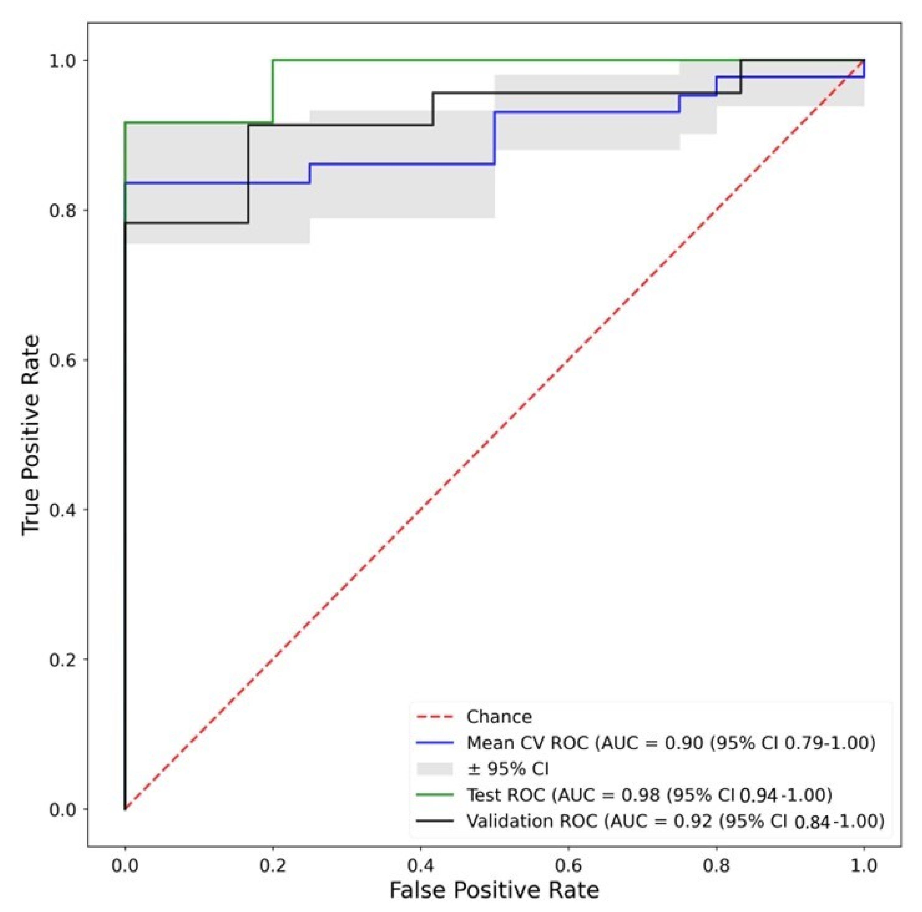
| Fingerprint A -Random Forest | 0.74 | 0.90 (0.79–1.00) | 0.8 | 0.98 (0.94–1.00) | 0.75 | 0.92 (0.84–1.00) |
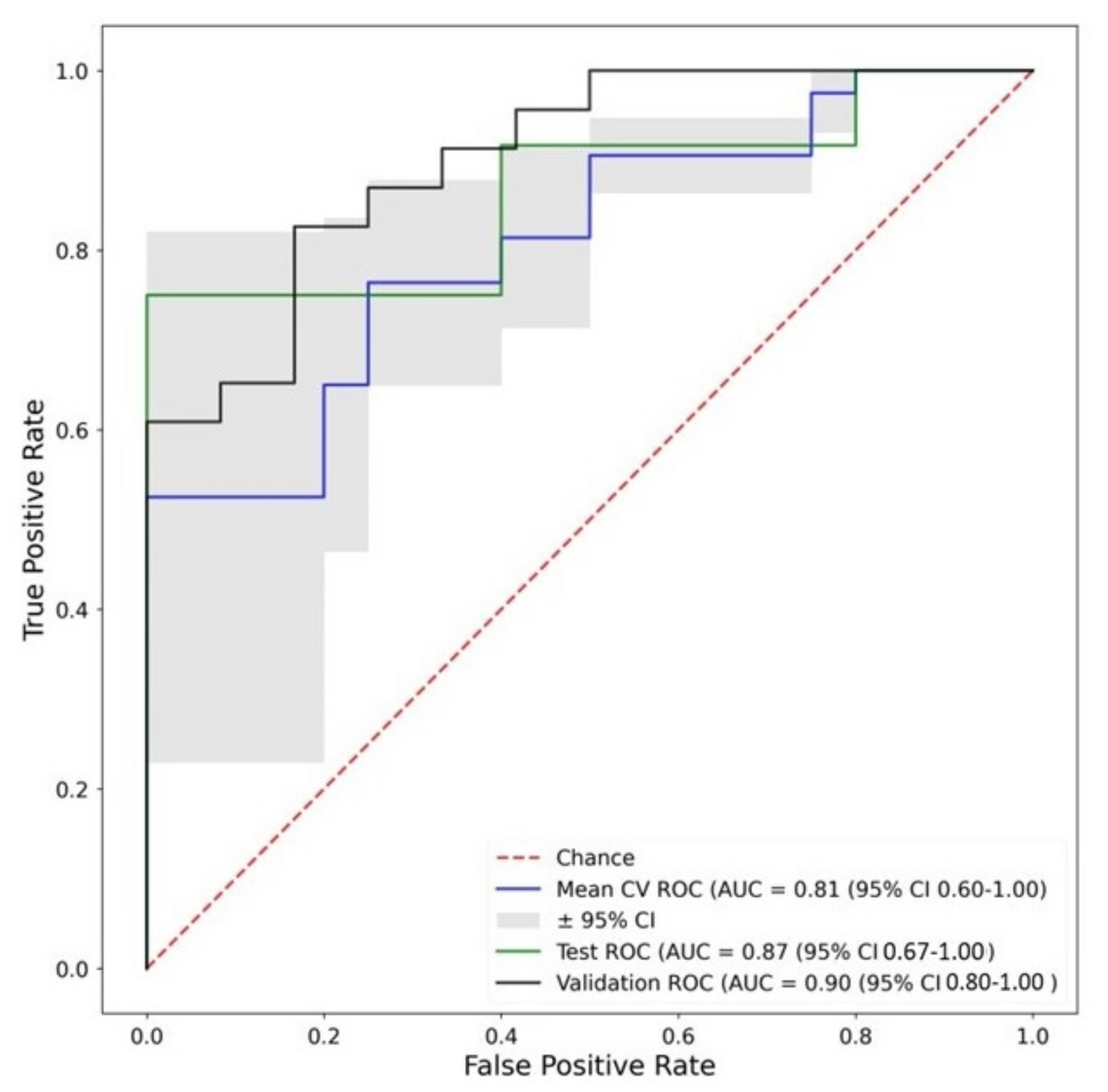
| Fingerprint B -Neural Net | 0.66 | 0.81 (0.60–1.00) | 0.68 | 0.87 (0.67–1.00) | 0.81 | 0.90 (0.80–1.00) |
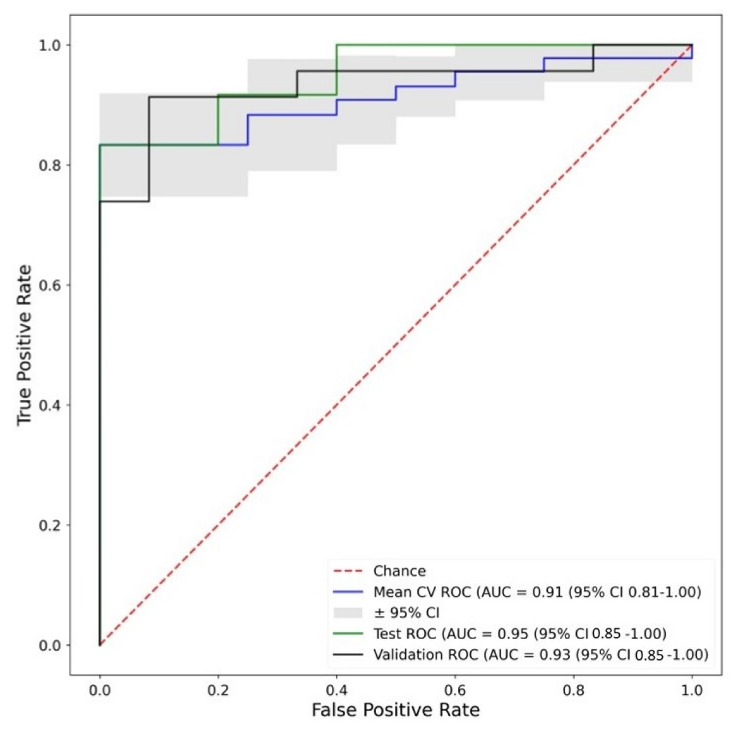
| Fingerprint C -Random Forest | 0.79 | 0.91 (0.81–1.00) | 0.8 | 0.95 (0.85–1.00) | 0.73 | 0.93 (0.85–1.00) |
| Qualitative Assessment | Literature AUC 0.81–0.98 [11] | |||||
|---|---|---|---|---|---|---|
| Training Accuracy | Training AUC (95% CI) | Testing Accuracy | Testing AUC (95% CI) | Validation Accuracy | Valdiation AUC (95% CI) | |
| SUV Feature -SUV 90th Percentile | 0.69 | 0.86 (0.66–1.00) | 0.7 | 0.93 (0.79–1.00) | 0.67 | 0.83 (0.68–0.99) |
| Radiomic Feature—GLDM Small Dependence High Gray Level Emphasis | 0.66 | 0.85 (0.73–0.97) | 0.8 | 0.98 (0.94–1.00) | 0.77 | 0.82 (0.67–0.96) |
| Fingerprint A—Logistic Regression | 0.76 | 0.86 (0.69–1.00) | 0.72 | 0.90 (0.75–1.00) | 0.79 | 0.93 (0.86–1.00) |
| Fingerprint B—Neural Net | 0.64 | 0.74 (0.57–0.91) | 0.72 | 0.90 (0.75–1.00) | 0.77 | 0.90 (0.80–1.00) |
| Fingerprint C—Random Forest | 0.81 | 0.88 (0.72–1.00) | 0.62 | 0.88 (0.71–1.00) | 0.7 | 0.89 (0.79–1.00) |
| Manual Segmentation Training AUC Mean (95% CI) | Automated Segmentation Training AUC Mean (95% CI) | |
|---|---|---|
| SUV Feature—SUV 90th Percentile | 0.85 (0.77–0.93) | 0.86 (0.81–0.91 ) |
| Radiomic Feature—GLSZM High Gray Level Zone Emphasis/GLCM Difference Variance | 0.91 (0.84–0.98 ) | 0.89 (0.87–0.91 ) |
| Fingerprint A—Random Forest | 0.91 (0.80–1.0 ) | 0.85 (0.81–0.89 ) |
| Fingerprint B—Random Forest/Support Vector Machine | 0.88 (0.81–0.95 ) | 0.91 (0.84–0.98 ) |
| Fingerprint C—Random Forest | 0.86 (0.78–0.94 ) | 0.81 (0.74–0.89 ) |
| Non-Harmonized | Harmonized | |||
|---|---|---|---|---|
| Validation Accuracy | Validation AUC (95% CI) | Validation Accuracy | Validation AUC (95% CI) | |
| SUV Feature—SUV Mean | 0.6 | 0.72 (0.62–0.83) | 0.59 | 0.72 (0.61–0.82) |
| Radiomic Feature—First Order Energy/GLDM Dependence Entropy | 0.63 | 0.72 (0.61–0.82) | 0.58 | 0.83 (0.75–0.91) |
| Fingerprint A—Random Forest/K Nearest Neighbours | 0.71 | 0.80 (0.71–0.89) | 0.69 | 0.72 (0.61–0.82) |
| Fingerprint B—Perceptron | 0.7 | 0.72 (0.61–0.82) | 0.7 | 0.70 (0.59–0.81) |
| Fingerprint C—Random Forest | 0.48 | 0.61 (0.50–0.72) | 0.6 | 0.68 (0.57–0.78) |
Disclaimer/Publisher’s Note: The statements, opinions and data contained in all publications are solely those of the individual author(s) and contributor(s) and not of MDPI and/or the editor(s). MDPI and/or the editor(s) disclaim responsibility for any injury to people or property resulting from any ideas, methods, instructions or products referred to in the content. |
© 2023 by the authors. Licensee MDPI, Basel, Switzerland. This article is an open access article distributed under the terms and conditions of the Creative Commons Attribution (CC BY) license (https://creativecommons.org/licenses/by/4.0/).
Share and Cite
Duff, L.M.; Scarsbrook, A.F.; Ravikumar, N.; Frood, R.; van Praagh, G.D.; Mackie, S.L.; Bailey, M.A.; Tarkin, J.M.; Mason, J.C.; van der Geest, K.S.M.; et al. An Automated Method for Artifical Intelligence Assisted Diagnosis of Active Aortitis Using Radiomic Analysis of FDG PET-CT Images. Biomolecules 2023, 13, 343. https://doi.org/10.3390/biom13020343
Duff LM, Scarsbrook AF, Ravikumar N, Frood R, van Praagh GD, Mackie SL, Bailey MA, Tarkin JM, Mason JC, van der Geest KSM, et al. An Automated Method for Artifical Intelligence Assisted Diagnosis of Active Aortitis Using Radiomic Analysis of FDG PET-CT Images. Biomolecules. 2023; 13(2):343. https://doi.org/10.3390/biom13020343
Chicago/Turabian StyleDuff, Lisa M., Andrew F. Scarsbrook, Nishant Ravikumar, Russell Frood, Gijs D. van Praagh, Sarah L. Mackie, Marc A. Bailey, Jason M. Tarkin, Justin C. Mason, Kornelis S. M. van der Geest, and et al. 2023. "An Automated Method for Artifical Intelligence Assisted Diagnosis of Active Aortitis Using Radiomic Analysis of FDG PET-CT Images" Biomolecules 13, no. 2: 343. https://doi.org/10.3390/biom13020343