
Attosecond Time Delay Trends across the Isoelectronic Noble Gas Sequence
Department of Physics, The Ohio State University, Columbus, OH 43210, USA
*
Author to whom correspondence should be addressed.
Atoms 2023, 11(5), 84; https://doi.org/10.3390/atoms11050084
Submission received: 28 February 2023
/
Revised: 10 May 2023
/
Accepted: 12 May 2023
/
Published: 15 May 2023
(This article belongs to the Special Issue Photon and Particle Impact Spectroscopy and Dynamics of Atoms, Molecules, and Clusters)
Abstract
:The analysis and measurement of Wigner time delays can provide detailed information about the electronic environment within and around atomic and molecular systems, with one the key differences being the lack of a long-range potential after a halogen ion undergoes photoionization. In this work, we use relativistic random-phase approximation to calculate the average Wigner delay from the highest occupied subshells of the atomic pairings (2p, 2s in Fluorine, Neon), (3p, 3s in Chlorine, Argon), (4p, 4s, 3d, in Bromine, Krypton), and (5p, 5s, 4d in Iodine, Xenon). The qualitative behaviors of the Wigner delays between the isoelectronic pairings were found to be similar in nature, with the only large differences occurring at photoelectron energies less than and around Cooper minima. Interestingly, the relative shift in Wigner time delays between negatively charged halogens and noble gases decreases as atomic mass increases. All atomic pairings show large differences at low energies, with noble gas atoms showing large positive Wigner delays, while negatively charged halogen ions show negative delays. The implications for photoionization studies in halide-containing molecules is also discussed.
1. Introduction
The recent advancement of attosecond extreme ultraviolet infrared (XUV-IR) laser metrology over the past decade [1,2,3,4,5,6] has enabled access for observing ultrafast phenomena across a variety of atomic and molecular systems at the natural time scale of their electronic motion. One common experimental technique utilizes an XUV-IR pump–probe process [7,8], where an electron is first ionized through the absorption of an XUV photon and subsequently streaked by the few-cycle IR laser field, which imprints itself on the photoelectron’s final energy and momentum. By varying the time delay between the XUV and IR pulses, it is possible to measure the photoionization time delay relative to a reference. Another common technique is reconstruction of attosecond beating by interference of two-photon transitions (RABBITT) [9,10], where the target is first ionized by an XUV attosecond pulse train of high-order harmonics, and the photoelectron can then either absorb or emit a secondary IR photon in the continuum. By adjusting the delay between the IR laser field and the high-order harmonics, it is possible to extract the time delay for a particular transition.
These techniques have been used to measure photoionization delays in atoms [11,12,13,14,15], molecules [16,17,18,19,20], and solid-state systems [21,22,23], thereby providing new information about their electronic structure. The total time delay , also known as the streaking delay, given by a pump-probe experiment is frequently separated into two components, . This convention of separating the total delay into two separate terms is also followed in traditional RABBITT experiments, with the only difference being that is replaced by the continuum–continuum delay [10].The first contribution is the Wigner time delay [24,25] , which describes the group delay of the ionized photoelectron due to the absorption of an XUV photon and depends on the nature of the target. The second component is the Coulomb-laser coupling time delay [26] , as it describes the delay caused by the coupling between the IR field in the continuum and the long-range potential of the remaining ion. Unlike the Wigner time delay, which requires an accurate description of the target potential, the Coulomb-laser coupling delay can be computed with an analytical formula [26,27,28] and does not rely on the precise nature of the target species. It does, however, depend on the photoelectron’s kinetic energy, the energy of the photons from the laser, and the charge of the residual ion. For example, the photoionization of a neutral atom will create a positively charged ion of and, therefore, will be finite, but if a negatively charged halogen undergoes photoionization, the remaining ion will have a neutral charge and will vanish. This implies that it is possible to directly measure the Wigner delay of negatively charged halogen ions.
The process of removing an electron from a neutral atom is called photoionization, while the removal of an electron from a negatively charged ion is called photodetachment. Many theoretical and experimental studies have been conducted to accurately describe and predict various aspects of the photoionization process in noble gas atoms (with some of the key features being photoemission angle dependence [29,30,31,32], autoionization resonances [33], the 4d giant dipole resonance in Xenon [34], photorecombination [35], and relativistic effects [36,37,38]) but only recently has work been conducted on Wigner time delays in negatively charged species [39,40,41,42,43,44,45].
This understanding of the time delays of negatively charged halogens is important for two key reasons. First, the halides are isoelectronic to the well-studied systems of , respectively, and, hence, they allow for an interesting comparison of two systems where the initial electronic configurations are identical and yet the binding energies significantly differ. Second, it has been shown that in the case of iodine-containing molecules, such as methyl iodide [46], the 4d orbitals of iodide are non-bonding and reasonably agree with the predicted cross-section data of an isolated iodine atom [47,48]. Therefore, comparisons between the Wigner delays in halogen ions and noble gases should help to inform future molecular photoionization studies while also helping to confirm the driving mechanisms behind Wigner time delay phenomena.
In this paper, we utilize the relativistic random-phase approximation (RRPA) formalism of Johnson and Lin [49] to calculate the average phases and average Wigner time delays of the highest occupied s, p, and d shells of the noble gas series and their halide counterparts. The theoretical details of RRPA are given in Section 2, along with a description of the methodology used to calculate the average Wigner time delays, the results of which are illustrated in Section 3, with the time delays of each halide–noble gas pairing being plotted with respect to photoelectron kinetic energy. Section 3 also includes a discussion regarding the similar qualitative behavior in the known regions of the Cooper minimum, while also acknowledging the sharp contrast in time delays at photoelectron energies below for the highest occupied p and s orbitals. The first part of Section 3 briefly describes the methodology used to calculate the Dirac–Hartree–Fock orbitals and their associated binding energies, along with specific details regarding the number of photoionization channels used for the RRPA calculations of each atom. Section 4 provides a summary of the results and a brief discussion regarding applications for future molecular ionization studies.
2. Theoretical Overview of the Relativistic Random-Phase Approximation (RRPA)
The same theoretical formalism was applied to negative halogen ions and neutral noble gas atoms in order to calculate the photoionization dipole transition matrix amplitudes and phases for an initial bound state. This overview follows the same outline as the previous RRPA photoionization studies of Kheifets and Deshmukh [50] and the original multi-channel paper of Johnson and Lin [49]. Atomic units ( are used throughout, unless stated otherwise.
For a time-dependent perturbation of the form , the probability amplitude for a transition from the ground state to an excited state , stimulated by said perturbation, is given by
For an electromagnetic interaction described in the Coulomb gauge, it is possible to rewrite the transition amplitude as a function of the vector potential , where the perturbations are described by, with .
Therefore, a photon of frequency (or equivalently of wavevector ) and polarization can be described by the vector potential in the Coulomb gauge as , which can then be expanded in terms of its multipole components, . Note that an upper index of corresponds to the electric and magnetic multipoles, respectively. In the single active electron approximation, the transition amplitude describe by Equation (2) can be reduced even further to
where and are the angular momentum quantum numbers describing the incoming photon. It is common to label the initial bound state of the electron by the quantum numbers and the final continuum state by the numbers . The spin of the electron is given by the spinor , where . Any final state can be uniquely described by the index , where is the total angular momentum of the outgoing electron in the continuum. The final state can also be written as a partial wave expansion, which is given explicitly in Equation (40) of [49]. Inserting this expansion into Equation (3) results in
The ionized photoelectron’s energy and momentum are represented by and , respectively, while is described in terms of Clebsch–Gordan coefficients and spherical harmonics.
The six-term bracket to the right of the in Equation (4) corresponds to the Wigner 3-j symbol, and represents the reduced matrix element describing the transition from the initial state to the final state multiplied by the phase shift of the continuum photoelectron wave .
One should note that the electric (or magnetic) multipole operator in the reduced matrix element is the only component that changes in Equation (4) for different values of , as the entire matrix element can be deconstructed as
where is a radial integral listed in [49] and is simply the parity factor responsible for imposing the necessary selection rules for a given transition.
Despite its use for describing single-electron transitions, Equation (4) is also valid for any closed-shell atomic species, as the only change required in Equations (4) and (6) is that the single-electron reduced matrix element is modified slightly to include multi-electron RRPA effects in both the initial and final states. An explanation of this modification is given in Appendix A.
In this work, we restrict ourselves to electric dipole transitions with linearly polarized light oriented along the axis . From these restrictions, Equation (4) simplifies to
Here, we have followed the convention of ref. [51] by defining separate transition amplitudes for the spin-up and spin-down cases and by omitting the scaling factor of . By choosing the linear polarization of the incoming photon to be purely along , it is possible to take advantage of the axial symmetry of the system. Therefore, we will introduce the shorthand , where corresponds to a photoelectron emission parallel to the direction of the initial photon.
It useful to observe how Equation (10) directly reduces in the simple case of electric dipole transitions for the and states. The expressions for the and transition amplitudes can be found in ref. [50].
The reduced matrix elements can be evaluated numerically for both its real and imaginary components, as doing so allows for the phase and Wigner time delay to be calculated using the standard formulation of
For a given subshell , the angle-dependent time delay can be calculated as a weighted average over all possible transition amplitudes and spin states.
For the purposes of this work, we will only consider the case of , as it is commonly the most dominant direction of photoelectron emission. As with Equation (10), it is informative to see how Equation (14) simplifies into the simple weighted average of the spin-up and spin-down Wigner delays for the case of an state.
This process of averaging Wigner delays was performed for every subshell listed in Table 1 below. By taking the average Wigner delays and and weighting them by their respective differential cross-sections, the total average time delay was also calculated. An analogous process was also used to compute and for every halogen and noble gas.
It should be noted that the accuracy of this averaging process depends not only on the values of the Wigner delays, but also with regard to the accuracy of the transition amplitudes themselves. Because the photoionization cross-section can be computed from the transition amplitudes , it is possible to estimate the accuracy of the RRPA calculations by simply comparing the predicted cross-sections with those of experimental measurements. Reference [38] lists the predicted RRPA cross-sections for all of the noble gases being studied in this work, and found there to be a good agreement with experimental values. This result implies that the calculated RRPA transition amplitudes given by Equation (10) should also be quite accurate.
3. Results and Discussion
In this section, we present the calculated binding energies and average Wigner delays for each of the highest subshells of the halide ions and noble gas atoms. It should be noted that RRPA often produces autoionization resonances in the time delay spectra for any given noble gas. However, they are not the focus of this paper and, therefore, have been filtered out to prevent the obfuscation of more general time delay features. The locations of autoionization resonances in noble gases are well documented [38], but they generally occur at photon energies close to the binding energies of orbital subshells. In Argon, for example, the autoionization resonances produced by RRPA occur around photon energies of , which corresponds to the ionization threshold of the subshell.
3.1. Dirac–Hartree–Fock (DHF) Orbital Subshell Ionization Calculations
RRPA requires the use of Dirac–Hartree–Fock orbitals in order to account for ab initio relativistic effects and to obtain accurate subshell ionization potential energies. It is important to note that DHF calculations are typically the most accurate for the highest occupied shells regardless of the atom being studied; however, they can reasonably predict the binding energy of lower-lying subshells as atomic mass increases. Table 1 confirms this trend, as the predicted value of the 4d orbitals in xenon are within ~ of experimental measurements. The binding energies of halide ions are not well known, yet it is possible to approximate their highest experimental binding energies with electron affinity measurements. The electron affinity values were found to closely match the calculated DHF energies, with the approximation being increasingly valid for the higher-mass ions of bromide and iodide. These trends and absolute energies were also found to agree with the calculated values of Saha et al. [38,41] and Lindroth and Dahlstrom [39]. The congruence between our calculated DHF binding energy for and the energy reported in [39], which utilized a non-relativistic HF theory with exchange, is of particular interest as it implies that despite not being necessary, relativistic effects do not negatively impact Wigner time delay calculations for lighter-mass atomic systems.

Table 1 also lists the number of coupled photoionization channels used for the subsequent calculations of the reduced matrix elements. For Neon and Fluorine, all nine possible channels () were coupled. Argon and Chlorine used 14 channels () and omitted the channels. Krypton and Bromine used 20 channels () and omitted the channels. Finally, Xenon and Iodine used 33 channels () and omitted the core channels. The omitted channels could be ignored due to the fact that they are significantly farther away in energy from the other channels and do not have substantial impact at the photon energies of this study.
3.2. Individual Photoionization Channel Phases and Wigner Time Delays of Neon and
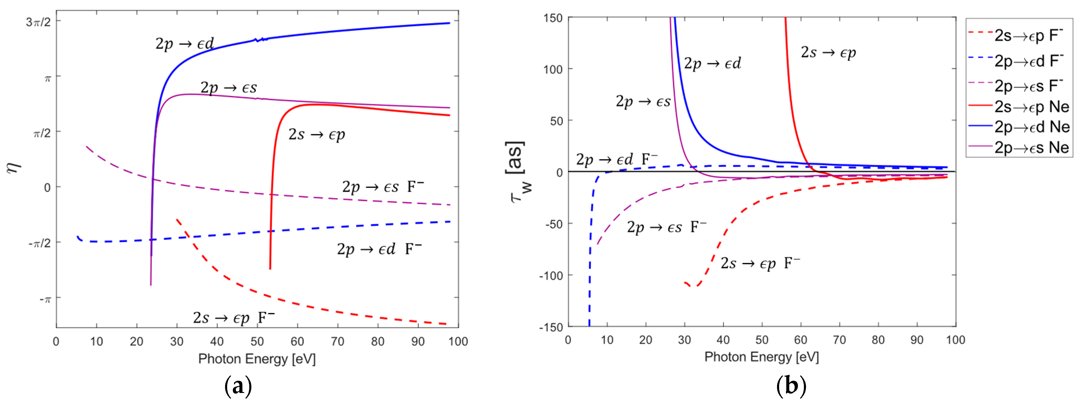
While a previous study compared the Wigner delays of individual ionization channels in Argon and Chlorine [41], to the best of our knowledge, no similar study has been performed for the lighter pair of Neon and Fluorine. The phase of each channel was calculated directly by computing the argument of the reduced matrix element associated with each channel (i.e., via Equations (6) and (13)). By simply taking the energy derivative of the phase, the Wigner time delays could also be determined, as seen in Figure 1. Due to their low atomic mass and relatively small number of electrons, relativistic effects do not play a crucial role in time delays in Neon and Fluorine. This is reflected in the behavior of both the phase and Wigner time delays for any given channel, since the and values of a particular transition have a negligible impact (e.g., the and both produce the same and Wigner delay). This fact also holds true for the and channels in both Chlorine and Argon [41], but begins to break down for the lower-lying and channels. While not the primary focus of this work, the study of time delays in individual channels is often useful for analyzing the results of the average orbital delays, since it is possible to determine where a given channel dominates in a particular energy region and instructive to see how the average delay results from Wigner delays of individual transitions. For the sake of brevity, the individual channel phases and time delays for are omitted.
By comparing Figure 1b and Figure 2b, it is apparent that the average delay in Ne is dominated by the channels across all photon energies, whereas the average delay in primarily corresponds to transitions at higher energies and channels below photon energies near . This agrees with the fact that for typical photoionization in noble gases, the photoionization channels are known to dominate regardless of energy, with the only exception being Cooper minima. However, in photodetachment, the channels dominate near the threshold and the channels only begin to dominate once photon energy increases [41,45]. A cursory comparison of the time delays between Neon and Fluorine shows a strong agreement for photon energies greater than for any given transition. The same can also be said of transitions at photon energies above . There is, however, a sharp contrast between the time delays at lower energies.
3.3. Comparison of Average Wigner Delays for Halogen Ions and Noble Gases
We observe in Figure 2a,b that Neon exhibits the familiar time delay behavior of having a large positive delay near the threshold energies of the and subshells, which slowly vanishes as photon energy increases. Fluorine, by contrast, exhibits a strong negative delay on the order of near the threshold. This difference can be explained by comparing the differences in the calculated phases for both Fluorine and Neon illustrated in Figure 1a, as each of Neon’s ionization channels displays a dramatic increase near their respective threshold energies, while Fluorine’s and channels tend to decrease more gradually over a longer energy range. For noble gas atoms, the Wigner time delay of any given orbital will trend towards positive infinity at energies near the threshold due to the drastic increase in the Coulomb phase, which is known to dominate [40,41], and the individual channels of Ne confirm this trend. The Coulomb phase for negatively charged atoms is essentially nonexistent due to the lack of a long-range Coulomb potential and, therefore, the Wigner delays corresponding to photodetachment do not possess the same behavior of trending towards infinity at low energies. In the case of photodetachment, however, it is still possible for a short-range potential to play a role at energies extremely close to the threshold. For example, in Figure 1a, the phase of the ionization channels in Fluorine rapidly decreases in an energy region of near threshold and then slowly increases with photon energy. This also explains the sharp increase in the average Wigner delays in Fluorine at low photoelectron energies below and small positive delay times in the higher photoelectron energy region.
Just as with the individual channel analysis in Fluorine and Neon, we find that the average and Wigner delays also diverge at lower photoelectron energies and converge towards zero in the large photoelectron kinetic energy limit. The physical picture underlying this vanishing time delay is quite clear, as a photoelectron with high kinetic energy will spend less time near the perturbative effects of the remaining ion and instead behave more similarly to a free electron wave. Conversely, at low kinetic energies, the photoelectron will spend more time near the remaining ion and be more susceptible to collective electron effects. We also observe the same general feature of diverging Wigner delays between the and states in Chlorine and Argon at low energy (see Figure 2c,d), with the only difference being the introduction of Cooper minima. A Cooper minimum occurs when the transition matrix element changes sign and undergoes a phase shift of . Typically, this happens when the initial state radial wavefunction contains at least one node and overlaps with the continuum wavefunctions. This is the process responsible for the well-known Cooper minima illustrated for Argon and Chlorine in Figure 2d. However, a different mechanism is responsible for the observed minimum in the average Wigner delay of Argon and Chlorine. Instead of being the result of a radial node in the initial wavefunction, the behavior of the Cooper minimum in the 3s channel is caused by a shift in the phases of the channels, which occurs due to the result of significant interchannel coupling with the ionization channels [38,56,57]. Without the effect of interchannel coupling, this minimum does not appear in the ionization channels, which is why the minimum can be deemed an “induced Cooper minimum” as it is still the result of a shift but its origin differs from that of the Cooper minimum. However, the location of this induced Cooper minimum in Chlorine appears to be shifted higher than the induced Cooper minimum in Argon. A similar shift occurs for the Cooper minimum [58] in the spectra, with Chlorine again displaying a higher shift of . Because Figure 2 plots both time delays with respect to the kinetic energy of the ionized electron, any difference in the location of the two Cooper minima must be the result of properties not related to the threshold energies of the atomic systems. If the shift was solely caused by a difference in binding energies, the two Wigner delay spectra would overlap.
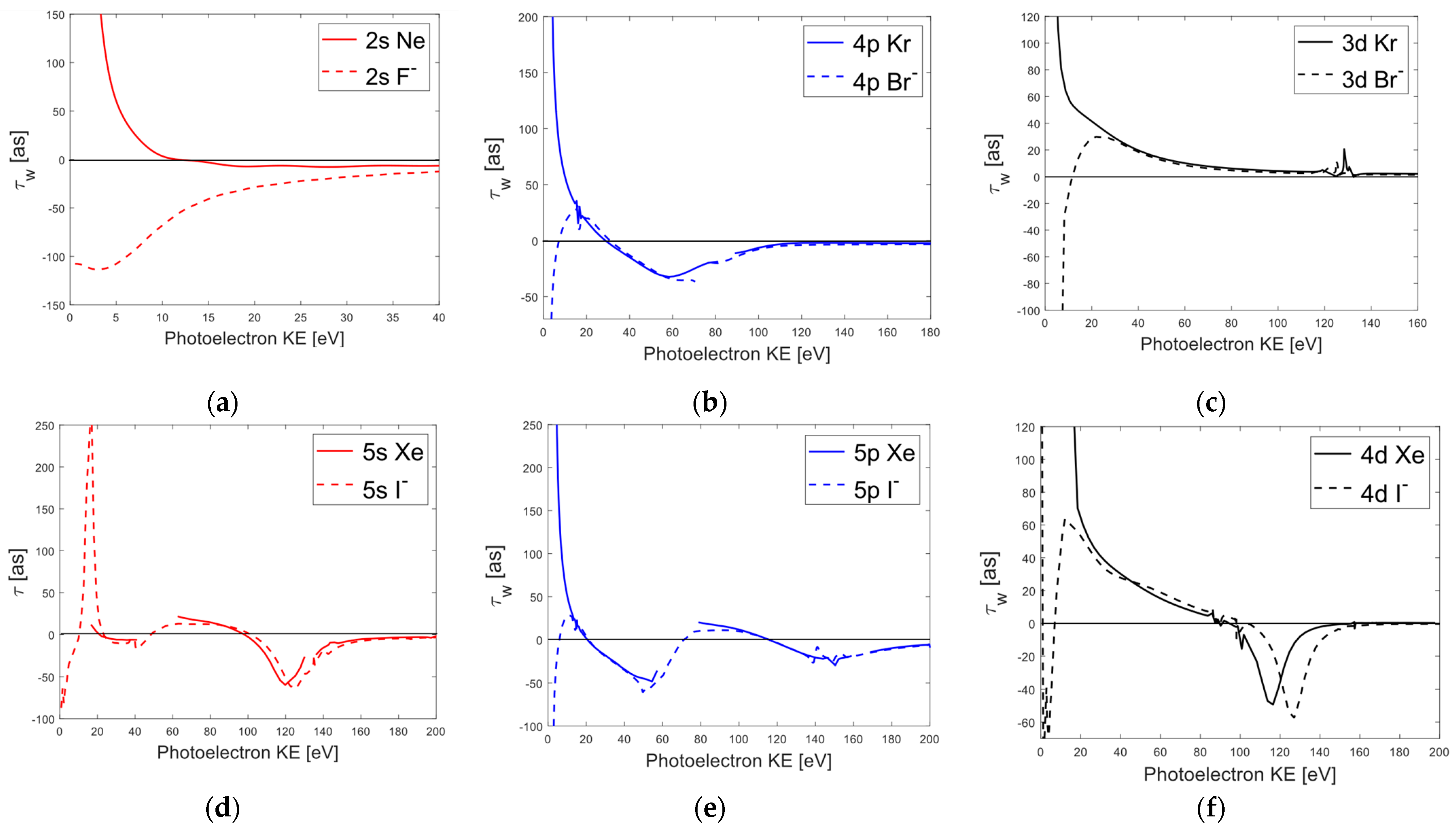
For the higher-mass systems of Bromine, Krypton, Iodine, and Xenon illustrated in Figure 3, the average Wigner time delays for each orbital were also found to diverge at low photoelectron energies, as and both display large negative time delays (again on the order of ) in the low energy region. This appears to indicate a universal time delay trend between negative charged halogens and noble gas atoms at photoelectron energies below . While it is possible to explain the negative delay times as the result of a negative energy derivative of the phase, a physical explanation is less obvious. If one interprets a positive delay time as the retardation of the photoelectron wave with respect to a free electron wave of the same kinetic energy, then a negative Wigner delay can be interpreted as an acceleration in the outgoing electron wave packet. In the case of the induced Cooper minimum in the average 3s state for Argon at low energy, the “dip” in the delay time can be thought to be the result of induced oscillations in the outer subshells that screen the electrons [57]. This only can occur for systems where the states are strongly coupled, which explains the absence of a similar feature in the time delay spectra of Neon due to its and interchannel coupling being much weaker.
The Cooper minima in the average Wigner delay for Xenon have also been explained to be the result of interchannel couplings, with the first Cooper minimum near being the result of couplings with the and states and the second minimum at being the result of couplings with the and states [59,60]. In the case of , we also find the same Cooper minima at energies approximately equal to those of Xenon. A similar equivalence was observed between the average Wigner delays of Iodine and Xenon, as well as for the delays in and . However, the minimum in the time delay spectra for was found to lie higher than for non.
Comparing the relative shifts between Cooper minima for the average Wigner delays of each halogen and noble gas pairing, we find a qualitative trend where the difference decreases as atomic mass increases. The origin of this trend is still not entirely clear, although it could be related to the relative difference in the electronegativities and polarizabilities of the halogen and noble gas atoms, as relative shifts have been observed in the photodetachment cross-sections for different isotopes of Chlorine [61]. A previous theoretical study [62] also reported shifts in the respective and cross-sections for and and other high-Z isoelectronic species that were positively charged (i.e., , ) and concluded that interchannel coupling and initial-state correlation effects can impact the location of Cooper minima, although they do not directly account for the difference in binding energies between and . Despite not focusing on the relative shift in photoionization cross-sections, our work regarding the Wigner delays between and seems to agree with the conclusions of [62], since the location and appearance of an “induced Cooper minimum” in Figure 2c was found to be the result of significant coupling to the ionization channels in Argon. However, more work must be carried out to determine the origin for the relative shift in the Cooper minima between isoelectronic systems.
4. Conclusions
In this work, we performed RRPA Wigner time delay calculations for the halogen ion and noble gas pairings of . The individual photoionization channels were then averaged to obtain the average delay times for the highest occupied states. The Wigner delays were plotted with respect to photoelectron energy in order to account for energy shifts due to differences in binding energies. For photoelectron energies below , negatively charged halogen ions exhibit large negative Wigner delays that sharply increase. This qualitative difference is due to the absence of a large Coulomb phase, which is known to dominate the Wigner delay behavior of noble gases at low energies. Overall, the qualitative time delay behaviors of halogens and noble gases were found to be similar, with each pairing displaying the same general features and Cooper minima. The location of the Cooper minimum in was found to be shifted higher than . A similar shift of was noticed in the Wigner delays between . As atomic mass increased, this relative shift between Cooper minima was found to decrease, except in the case of the Cooper minima of , which displayed an shift above that of . The physical process underlying this relative shift is still not clear, indicating the need for more detailed analysis of negatively charged ions and noble gas atoms in the regions of Cooper minima. Molecular photoionization studies are becoming of greater interest to the attosecond community, with Iodine-containing molecules having already been favored due to iodine’s orbitals. Our findings indicate that the average Wigner delays of are the most similar to the average d orbital Wigner delays of their noble gas counterparts Kr and Xe. This implies that Bromine and Iodine are the best halogens for studying time delay phenomena in molecular systems.
Author Contributions
A.S.L. and B.G. conceptualized the study. B.G. performed the calculations and prepared the original draft. All authors have read and agreed to the published version of the manuscript.
Funding
This work was supported by the U.S. Department of Energy, Office of Basic Energy Sciences, Atomic, Molecular and Optical Sciences Program under Award No. DE-SC0022093.
Institutional Review Board Statement
Not applicable.
Informed Consent Statement
Not applicable.
Data Availability Statement
Simulation data can be provided upon reasonable request.
Acknowledgments
We thank Subhasish Saha for valuable discussions.
Conflicts of Interest
The authors declare no conflict of interest.
Appendix A. Determining
From Equation (3) in Section 2, it was possible to write the transition amplitude in terms of a single-electron reduced matrix element, , describing the transition between an initial state,, and final state, . In order to generalize this to the multi-electron case, one must start with Equation (2) and essentially repeat the same process that was carried out with the single-electron case (i.e., perform a multipole expansion of for both the positive frequency perturbations and negative frequency perturbation terms ).
It was the partial wave expansion given by Equation (40) in Johnson and Lin’s original paper [49] that, when substituted into Equation (3), resulted in the single-electron transition amplitude described by Equation (4). By following the same process of describing the final continuum state as a partial wave expansion, Equation (A1) leads to a generalized formula for the multi-electronic transition amplitude, which is identical to Equation (4) in Section 2, with the only necessary modification occurring to so that it now includes the multi-electron reduced matrix element.
where the reduced matrix element is now described by
Therefore, instead of considering only the transition between one set of waves and as was the case before with Equations (4) and (6), we are now summing all of the possible transitions between the remaining waves and under the condition that the waves vanish in the asymptotic limit . The reduced matrix elements are identical to the single-electron matrix elements in every way except in terms of the radial integral , which is given as Equation (46) in [49].
References
- Hentschel, M.; Kienberger, R.; Spielmann, C.; Reider, G.A.; Milosevic, N.; Brabec, T.; Corkum, P.; Heinzmann, U.; Drescher, M.; Krausz, F. Attosecond Metrology. Nature 2001, 414, 509–513. [Google Scholar] [CrossRef] [PubMed]
- Krausz, F. From Femtochemistry to Attophysics. Phys. World 2001, 14, 41. [Google Scholar] [CrossRef]
- Drescher, M.; Hentschel, M.; Kienberger, R.; Tempea, G.; Spielmann, C.; Reider, G.A.; Corkum, P.B.; Krausz, F. X-Ray Pulses Approaching the Attosecond Frontier. Science 2001, 291, 1923–1927. [Google Scholar] [CrossRef] [PubMed]
- Varjú, K.; Johnsson, P.; Mauritsson, J.; L’Huillier, A.; López-Martens, R. Physics of Attosecond Pulses Produced via High Harmonic Generation. Am. J. Phys. 2009, 77, 389–395. [Google Scholar] [CrossRef]
- Orfanos, I.; Makos, I.; Liontos, I.; Skantzakis, E.; Förg, B.; Charalambidis, D.; Tzallas, P. Attosecond Pulse Metrology. APL Photonics 2019, 4, 080901. [Google Scholar] [CrossRef]
- Frank, F.; Arrell, C.; Witting, T.; Okell, W.A.; McKenna, J.; Robinson, J.S.; Haworth, C.A.; Austin, D.; Teng, H.; Walmsley, I.A.; et al. Invited Review Article: Technology for Attosecond Science. Rev. Sci. Instrum. 2012, 83, 071101. [Google Scholar] [CrossRef]
- Itatani, J.; Quéré, F.; Yudin, G.L.; Ivanov, M.Y.; Krausz, F.; Corkum, P.B. Attosecond Streak Camera. Phys. Rev. Lett. 2002, 88, 173903. [Google Scholar] [CrossRef]
- Zaïr, A.; Mével, E.; Cormier, E.; Constant, E. Ultrastable Collinear Delay Control Setup for Attosecond IR-XUV Pump–Probe Experiment. J. Opt. Soc. Am. B JOSAB 2018, 35, A110–A115. [Google Scholar] [CrossRef]
- Klünder, K.; Dahlström, J.M.; Gisselbrecht, M.; Fordell, T.; Swoboda, M.; Guénot, D.; Johnsson, P.; Caillat, J.; Mauritsson, J.; Maquet, A.; et al. Probing Single-Photon Ionization on the Attosecond Time Scale. Phys. Rev. Lett. 2011, 106, 143002. [Google Scholar] [CrossRef]
- Vos, J.; Cattaneo, L.; Patchkovskii, S.; Zimmermann, T.; Cirelli, C.; Lucchini, M.; Kheifets, A.; Landsman, A.S.; Keller, U. Orientation-Dependent Stereo Wigner Time Delay and Electron Localization in a Small Molecule. Science 2018, 360, 1326–1330. [Google Scholar] [CrossRef]
- Kheifets, A.S. Wigner Time Delay in Atomic Photoionization. J. Phys. B At. Mol. Opt. Phys. 2023, 56, 022001. [Google Scholar] [CrossRef]
- Schultze, M.; Fieß, M.; Karpowicz, N.; Gagnon, J.; Korbman, M.; Hofstetter, M.; Neppl, S.; Cavalieri, A.L.; Komninos, Y.; Mercouris, T.; et al. Delay in Photoemission. Science 2010, 328, 1658–1662. [Google Scholar] [CrossRef]
- Palatchi, C.; Dahlström, J.M.; Kheifets, A.S.; Ivanov, I.A.; Canaday, D.M.; Agostini, P.; DiMauro, L.F. Atomic Delay in Helium, Neon, Argon and Krypton*. J. Phys. B At. Mol. Opt. Phys. 2014, 47, 245003. [Google Scholar] [CrossRef]
- Guénot, D.; Klünder, K.; Arnold, C.L.; Kroon, D.; Dahlström, J.M.; Miranda, M.; Fordell, T.; Gisselbrecht, M.; Johnsson, P.; Mauritsson, J.; et al. Photoemission-Time-Delay Measurements and Calculations Close to the 3s-Ionization-Cross-Section Minimum in Ar. Phys. Rev. A 2012, 85, 053424. [Google Scholar] [CrossRef]
- Kheifets, A.S.; Ivanov, I.A. Delay in Atomic Photoionization. Phys. Rev. Lett. 2010, 105, 233002. [Google Scholar] [CrossRef]
- Huppert, M.; Jordan, I.; Baykusheva, D.; von Conta, A.; Wörner, H.J. Attosecond Delays in Molecular Photoionization. Phys. Rev. Lett. 2016, 117, 093001. [Google Scholar] [CrossRef]
- Caillat, J.; Maquet, A.; Haessler, S.; Fabre, B.; Ruchon, T.; Salières, P.; Mairesse, Y.; Taïeb, R. Attosecond Resolved Electron Release in Two-Color Near-Threshold Photoionization of N2. Phys. Rev. Lett. 2011, 106, 093002. [Google Scholar] [CrossRef]
- Serov, V.V.; Kheifets, A.S. Time Delay in XUV/IR Photoionization of H2O. J. Chem. Phys. 2017, 147, 204303. [Google Scholar] [CrossRef]
- Baykusheva, D.; Wörner, H.J. Theory of Attosecond Delays in Molecular Photoionization. J. Chem. Phys. 2017, 146, 124306. [Google Scholar] [CrossRef]
- Haessler, S.; Fabre, B.; Higuet, J.; Caillat, J.; Ruchon, T.; Breger, P.; Carré, B.; Constant, E.; Maquet, A.; Mével, E.; et al. Phase-Resolved Attosecond near-Threshold Photoionization of Molecular Nitrogen. Phys. Rev. A 2009, 80, 011404. [Google Scholar] [CrossRef]
- Zhang, C.-H.; Thumm, U. Streaking and Wigner Time Delays in Photoemission from Atoms and Surfaces. Phys. Rev. A 2011, 84, 033401. [Google Scholar] [CrossRef]
- Borrego-Varillas, R.; Lucchini, M.; Nisoli, M. Attosecond Spectroscopy for the Investigation of Ultrafast Dynamics in Atomic, Molecular and Solid-State Physics. Rep. Prog. Phys. 2022, 85, 066401. [Google Scholar] [CrossRef] [PubMed]
- Tao, Z.; Chen, C.; Szilvási, T.; Keller, M.; Mavrikakis, M.; Kapteyn, H.; Murnane, M. Direct Time-Domain Observation of Attosecond Final-State Lifetimes in Photoemission from Solids. Science 2016, 353, 62–67. [Google Scholar] [CrossRef] [PubMed]
- Wigner, E.P. Lower Limit for the Energy Derivative of the Scattering Phase Shift. Phys. Rev. 1955, 98, 145–147. [Google Scholar] [CrossRef]
- Smith, F.T. Lifetime Matrix in Collision Theory. Phys. Rev. 1960, 118, 349–356. [Google Scholar] [CrossRef]
- Dahlström, J.M.; Guénot, D.; Klünder, K.; Gisselbrecht, M.; Mauritsson, J.; L’Huillier, A.; Maquet, A.; Taïeb, R. Theory of Attosecond Delays in Laser-Assisted Photoionization. Chem. Phys. 2013, 414, 53–64. [Google Scholar] [CrossRef]
- Dahlström, J.M.; Carette, T.; Lindroth, E. Diagrammatic Approach to Attosecond Delays in Photoionization. Phys. Rev. A 2012, 86, 061402. [Google Scholar] [CrossRef]
- Pazourek, R.; Nagele, S.; Burgdörfer, J. Time-Resolved Photoemission on the Attosecond Scale: Opportunities and Challenges. Faraday Discuss. 2013, 163, 353–376. [Google Scholar] [CrossRef]
- Wätzel, J.; Moskalenko, A.S.; Pavlyukh, Y.; Berakdar, J. Angular Resolved Time Delay in Photoemission. J. Phys. B At. Mol. Opt. Phys. 2014, 48, 025602. [Google Scholar] [CrossRef]
- Heuser, S.; Galán, Á.J.; Cirelli, C.; Marante, C.; Sabbar, M.; Boge, R.; Lucchini, M.; Gallmann, L.; Ivanov, I.; Kheifets, A.S.; et al. Angular Dependence of Photoemission Time Delay in Helium. Phys. Rev. A 2016, 94, 063409. [Google Scholar] [CrossRef]
- Cirelli, C.; Marante, C.; Heuser, S.; Petersson, C.L.M.; Galán, Á.J.; Argenti, L.; Zhong, S.; Busto, D.; Isinger, M.; Nandi, S.; et al. Anisotropic Photoemission Time Delays Close to a Fano Resonance. Nat. Commun. 2018, 9, 955. [Google Scholar] [CrossRef]
- Ivanov, I.A.; Kheifets, A.S. Angle-Dependent Time Delay in Two-Color XUV+IR Photoemission of He and Ne. Phys. Rev. A 2017, 96, 013408. [Google Scholar] [CrossRef]
- George, J.; Pradhan, G.B.; Rundhe, M.; Jose, J.; Aravind, G.; Deshmukh, P.C. Autoionization Resonances in the Argon Iso-Electronic Sequence. Can. J. Phys. 2012, 90, 547–555. [Google Scholar] [CrossRef]
- Magrakvelidze, M.; Madjet, M.E.-A.; Chakraborty, H.S. Attosecond Delay of Xenon 4d Photoionization at the Giant Resonance and Cooper Minimum. Phys. Rev. A 2016, 94, 013429. [Google Scholar] [CrossRef]
- Magrakvelidze, M.; Madjet, M.E.-A.; Dixit, G.; Ivanov, M.; Chakraborty, H.S. Attosecond Time Delay in Valence Photoionization and Photorecombination of Argon: A Time-Dependent Local-Density-Approximation Study. Phys. Rev. A 2015, 91, 063415. [Google Scholar] [CrossRef]
- Jordan, I.; Huppert, M.; Pabst, S.; Kheifets, A.S.; Baykusheva, D.; Wörner, H.J. Spin-Orbit Delays in Photoemission. Phys. Rev. A 2017, 95, 013404. [Google Scholar] [CrossRef]
- Keating, D.A.; Manson, S.T.; Dolmatov, V.K.; Mandal, A.; Deshmukh, P.C.; Naseem, F.; Kheifets, A.S. Intershell-Correlation-Induced Time Delay in Atomic Photoionization. Phys. Rev. A 2018, 98, 013420. [Google Scholar] [CrossRef]
- Saha, S.; Mandal, A.; Jose, J.; Varma, H.R.; Deshmukh, P.C.; Kheifets, A.S.; Dolmatov, V.K.; Manson, S.T. Relativistic Effects in Photoionization Time Delay near the Cooper Minimum of Noble-Gas Atoms. Phys. Rev. A 2014, 90, 053406. [Google Scholar] [CrossRef]
- Lindroth, E.; Dahlström, J.M. Attosecond Delays in Laser-Assisted Photodetachment from Closed-Shell Negative Ions. Phys. Rev. A 2017, 96, 013420. [Google Scholar] [CrossRef]
- Pi, L.-W.; Landsman, A.S. Attosecond Time Delay in Photoionization of Noble-Gas and Halogen Atoms. Appl. Sci. 2018, 8, 322. [Google Scholar] [CrossRef]
- Saha, S.; Jose, J.; Deshmukh, P.C.; Aravind, G.; Dolmatov, V.K.; Kheifets, A.S.; Manson, S.T. Wigner Time Delay in Photodetachment. Phys. Rev. A 2019, 99, 043407. [Google Scholar] [CrossRef]
- Saha, S.; Deshmukh, P.C.; Kheifets, A.S.; Manson, S.T. Dominance of Correlation and Relativistic Effects on Photodetachment Time Delay Well above Threshold. Phys. Rev. A 2019, 99, 063413. [Google Scholar] [CrossRef]
- Banerjee, S.; Deshmukh, P.C.; Kheifets, A.S.; Manson, S.T. Effects of Spin-Orbit-Interaction-Activated Interchannel Coupling on Photoemission Time Delay. Phys. Rev. A 2020, 101, 043411. [Google Scholar] [CrossRef]
- Saha, S.; Jose, J.; Deshmukh, P.C.; Kheifets, A.S.; Dolmatov, V.K.; Manson, S.T. Effects of Relativistic Interactions in Photodetachment Time Delay of Br−. J. Phys. Conf. Ser. 2020, 1412, 092013. [Google Scholar] [CrossRef]
- Banerjee, S.; Aarthi, G.; Saha, S.; Aravind, G.; Deshmukh, P.C. Time Delay in Negative Ion Photodetachment. Phys. Scr. 2021, 96, 114005. [Google Scholar] [CrossRef]
- Lindle, D.W.; Kobrin, P.H.; Truesdale, C.M.; Ferrett, T.A.; Heimann, P.A.; Kerkhoff, H.G.; Becker, U.; Shirley, D.A. Inner-Shell Photoemission from the Iodine Atom in CH3I. Phys. Rev. A 1984, 30, 239–244. [Google Scholar] [CrossRef]
- Magrakvelidze, M.; Chakraborty, H. Attosecond Time Delays in the Valence Photoionization of Xenon and Iodine at Energies Degenerate with Core Emissions. J. Phys. Conf. Ser. 2017, 875, 022015. [Google Scholar] [CrossRef]
- Biswas, S.; Förg, B.; Ortmann, L.; Schötz, J.; Schweinberger, W.; Zimmermann, T.; Pi, L.; Baykusheva, D.; Masood, H.A.; Liontos, I.; et al. Probing Molecular Environment through Photoemission Delays. Nat. Phys. 2020, 16, 778–783. [Google Scholar] [CrossRef]
- Johnson, W.R.; Lin, C.D. Multichannel Relativistic Random-Phase Approximation for the Photoionization of Atoms. Phys. Rev. A 1979, 20, 964–977. [Google Scholar] [CrossRef]
- Kheifets, A.; Mandal, A.; Deshmukh, P.C.; Dolmatov, V.K.; Keating, D.A.; Manson, S.T. Relativistic Calculations of Angle-Dependent Photoemission Time Delay. Phys. Rev. A 2016, 94, 013423. [Google Scholar] [CrossRef]
- Mandal, A.; Deshmukh, P.C.; Kheifets, A.S.; Dolmatov, V.K.; Manson, S.T. Angle-Resolved Wigner Time Delay in Atomic Photoionization: The 4d Subshell of Free and Confined Xe. Phys. Rev. A 2017, 96, 053407. [Google Scholar] [CrossRef]
- Kramida, A.; Ralchenko, Y.; Reader, J.; NIST ASD Team. NIST Atomic Spectra Database (Version 5.10), National Institute of Standards and Technology: Gaithersburg, MD, USA, 2022. Available online: https://physics.nist.gov/asd(accessed on 22 February 2023).
- NIST: Atomic Spectra Database—Energy Levels Form. Available online: https://physics.nist.gov/PhysRefData/ASD/levels_form.html (accessed on 22 February 2023).
- CCCBDB Electron Affinities. Available online: https://cccbdb.nist.gov/elecaff1x.asp (accessed on 22 February 2023).
- King, G.C.; Tronc, M.; Read, F.H.; Bradford, R.C. An Investigation of the Structure near the L2,3 Edges of Argon, the M4,5 Edges of Krypton and the N4,5 Edges of Xenon, Using Electron Impact with High Resolution. J. Phys. B At. Mol. Phys. 1977, 10, 2479. [Google Scholar] [CrossRef]
- Amusia, M.Y.; Ivanov, V.K.; Cherepkov, N.A.; Chernysheva, L.V. Interference Effects in Photoionization of Noble Gas Atoms Outer S-Subshells. Phys. Lett. A 1972, 40, 361–362. [Google Scholar] [CrossRef]
- Hammerland, D.; Zhang, P.; Bray, A.; Perry, C.F.; Kuehn, S.; Jojart, P.; Seres, I.; Zuba, V.; Varallyay, Z.; Osvay, K.; et al. Effect of Electron Correlations on Attosecond Photoionization Delays in the Vicinity of the Cooper Minima of Argon. arXiv 2019. Available online: https://arxiv.org/pdf/1907.01219 (accessed on 27 February 2023).
- Fano, U.; Cooper, J.W. Spectral Distribution of Atomic Oscillator Strengths. Rev. Mod. Phys. 1968, 40, 441–507. [Google Scholar] [CrossRef]
- Ganesan, A.; Banerjee, S.; Deshmukh, P.C.; Manson, S.T. Photoionization of Xe 5s: Angular Distribution and Wigner Time Delay in the Vicinity of the Second Cooper Minimum. J. Phys. B At. Mol. Opt. Phys. 2020, 53, 225206. [Google Scholar] [CrossRef]
- Aarthi, G.; Jose, J.; Deshmukh, S.; Radojevic, V.; Deshmukh, P.C.; Manson, S.T. Photoionization Study of Xe 5s: Ionization Cross Sections and Photoelectron Angular Distributions. J. Phys. B At. Mol. Opt. Phys. 2014, 47, 025004. [Google Scholar] [CrossRef]
- Berzinsh, U.; Gustafsson, M.; Hanstorp, D.; Klinkmüller, A.; Ljungblad, U.; Mårtensson-Pendrill, A.-M. Isotope Shift in the Electron Affinity of Chlorine. Phys. Rev. A 1995, 51, 231–238. [Google Scholar] [CrossRef]
- Jose, J.; Pradhan, G.B.; Radojević, V.; Manson, S.T.; Deshmukh, P.C. Electron Correlation Effects near the Photoionization Threshold: The Ar Isoelectronic Sequence. J. Phys. B At. Mol. Opt. Phys. 2011, 44, 195008. [Google Scholar] [CrossRef]
Figure 1.
Individual 2s and 2p channel phases (a) and Wigner time delays (b) for Neon and Fluorine. The individual labels are a descriptive shorthand to describe the identical behavior of multiple ionization channels. For instance, the label relates to the two ionization channels , while the label corresponds to the following three channels: . The behavior of is equivalent to the behavior of the channels. In the case of Ne, a small autoionization resonance was removed near 48 eV for the and channels.

Figure 2.
All four subfigures plot the average Wigner time delay with respect to the kinetic energy of the ionized electron. The first row compares the average Wigner time delays of Neon and Fluoride for the (a) and the (b) orbitals. The bottom row compares the average Wigner delays for Argon and Chloride with regard to their (c) and (d) orbitals. The resonant peaks in the Argon delay spectra between correspond to autoionization resonances that were not entirely removed. The average 3p Wigner delay for displays a deep minimum of −900 as near 6 eV. This minimum matches that of [41] although it is not shown due to the scale of the figure. The average and Wigner delays of and , respectively, originally displayed oscillations at photoelectron energies below 15 eV. These oscillations were determined to be caused by small variations in the average phase data and were subsequently removed by taking a best fit of the phase data and then computing the energy derivative of that best fit.

Figure 3.
Average Wigner time delays with respect to the kinetic energy of the ionized electron for Krypton and Bromide (a–c). Average Wigner time delays for the states of Xenon and Iodide (d–f). The autoionization resonances in and were removed at the approximate photon energies of . For and autoionization resonances were removed near .

Disclaimer/Publisher’s Note: The statements, opinions and data contained in all publications are solely those of the individual author(s) and contributor(s) and not of MDPI and/or the editor(s). MDPI and/or the editor(s) disclaim responsibility for any injury to people or property resulting from any ideas, methods, instructions or products referred to in the content. |
© 2023 by the authors. Licensee MDPI, Basel, Switzerland. This article is an open access article distributed under the terms and conditions of the Creative Commons Attribution (CC BY) license (https://creativecommons.org/licenses/by/4.0/).
Share and Cite
MDPI and ACS Style
Grafstrom, B.; Landsman, A.S. Attosecond Time Delay Trends across the Isoelectronic Noble Gas Sequence. Atoms 2023, 11, 84. https://doi.org/10.3390/atoms11050084
AMA Style
Grafstrom B, Landsman AS. Attosecond Time Delay Trends across the Isoelectronic Noble Gas Sequence. Atoms. 2023; 11(5):84. https://doi.org/10.3390/atoms11050084
Chicago/Turabian StyleGrafstrom, Brock, and Alexandra S. Landsman. 2023. "Attosecond Time Delay Trends across the Isoelectronic Noble Gas Sequence" Atoms 11, no. 5: 84. https://doi.org/10.3390/atoms11050084
Note that from the first issue of 2016, this journal uses article numbers instead of page numbers. See further details here.