
Characterization of a Continuous Beam Cold Atom Ramsey Interferometer

1
Department of Physics, U.S. Naval Academy, Annapolis, MD 21402, USA
2
Department of Physics, Naval Postgraduate School, Monterey, CA 93943, USA
*
Author to whom correspondence should be addressed.
Atoms 2023, 11(3), 51; https://doi.org/10.3390/atoms11030051
Submission received: 17 December 2022
/
Revised: 13 February 2023
/
Accepted: 19 February 2023
/
Published: 5 March 2023
(This article belongs to the Special Issue Advances in and Prospects for Matter Wave Interferometry)
Abstract
:The use of atom interferometers in inertial systems holds the promise of improvement of several orders of magnitude in sensitivity over sensors using current technology such as micro-electro-mechanical (MEMS) devices or ring laser gyroscopes (RLGs). This paper describes the construction and characterization of an atomic interferometry system for eventual use in a dual-atom-beam accelerometer/gyroscope sensor. In contrast with current state-of-the-art atomic sensors which use pulsed cold atom sources and pulsed laser beams, the investigated apparatus relies purely on continuous atomic and laser beams. These differences can result in a sensor with reduced complexity, a smaller physical footprint, and reduced power consumption. However, these differences also introduce challenges resulting from laser and atomic beam divergences and from velocity averaging due to both longitudinal and transverse velocity spreads. In this work, we characterize our rubidium-based atom beam system and show that Ramsey-style interference can still be observed. The implications for future research are also outlined and discussed.
1. Introduction
Atom interferometers were first demonstrated in 1991 with four near-simultaneous publications and follow-up articles [1,2,3,4,5]. Of these four demonstrations, three were performed using fast thermal beams of atoms [1,2,3] and one was performed using a pulsed, cold atom source [4,5]. Since then, a large number of groups have demonstrated atom interferometers of various types and several review articles have been written about atom interferometers, e.g., [6,7,8,9,10,11,12,13,14]. A large number of interferometers use a configuration whereby cold atoms are captured in a three-dimensional (3D) magneto-optical trap (MOT), launched in a controlled manner, and subjected to calibrated pulses of light; others use fast continuous beams of atoms subjected to light pulses [15,16,17]. There are, however, only a few reports of atom interferometers using continuous beams of atoms, moving at less-than-room-temperature thermal speeds, interacting with continuous beams of light for the atom optics [18,19].
It is well known that light pulse atom interferometer sensors are sensitive to both acceleration and rotation of the sensor platform [16,20]. The phase shift caused by acceleration and by rotation are given by
where k is the laser effective k-vector, a is the acceleration, T is the time between laser pulses (for pulsed systems; for continuous systems, this is the time it takes the atom to travel from one laser beam to the next), m is the mass of the atom, ℏ is the reduced Planck’s constant, is the rotation vector and is the area vector. In the absence of extraneous other phase shifts, the total phase shift in the interferometer then depends on the sum of the two phase shifts. Thus, for a single beam atom interferometer on a platform that is undergoing both linear acceleration and rotation at the same time, it is impossible to distinguish the contributions to the total phase with a single measurement. However, the contribution that arises from rotation changes sign when the direction of the atoms is reversed, but the contribution from the acceleration phase shift does not. Thus, a dual-beam atom interferometer with two atom sources opposing each other and a common interferometry region can unambiguously measure both the contributions from the acceleration phase shift and the rotation phase shift. The sum of the outputs of the two interferometers will depend solely on acceleration, while the difference in the two outputs will depend purely on rotation. Pulsed versions of these types of sensors are explained in greater detail in [16,20].
The use of pulsed atomic and optical sources does have advantages over continuous sources. The atom sources are typically bright (in the order of 1 billion atoms per shot). The length of time the atoms are exposed to the optical fields is very precisely determined by the optical pulse length and is under the control of the experimentalist. The divergence of the atoms as they travel through the interferometer is determined by the temperature of the atoms and is again largely under the control of the experimentalist. On the other hand, due to the velocity spread of the atoms in continuous beam interferometers, the pulse time as seen by the atoms is not uniform, and the divergence of the atoms from a two-dimensional (2D) MOT can be large. Despite these drawbacks, continuous sources have several practical advantages especially from the perspective of fieldable devices. Using atoms that emerge from a relatively “simple” 2D-MOT avoids the complexity of building a 3D-MOT. Pulsed atom sources require precise timing to launch atoms, apply Raman pulses, and measure the results as the atoms pass a detection region, and the detection laser must be pulsed on at the correct time. Typically, pulsing light beams on and off is achieved by passing the light through an acousto-optic modulator and pulsing the driving radio frequency on and off. Ultimately, a system that depends on loading a 3D-MOT is more complicated, requires complex timing, and is a pulsed system which can lead to dead time issues in an eventual sensor. Therefore, it is of importance to explore atom sources for atom interferometry that employ continuous cold atom sources and continuous optical fields, with overall reduced complexity, and physical footprint as the primary design considerations. Additionally, minor power savings can be realized by using fewer modulators.
Continuous cold-beam sources for the purpose of atom interferometry have been explored before [18,19]. However, in studies such as the one reported on in [18] the so-called low-velocity intensity source (LVIS) method was used to generate a beam of continuous cold atoms [21]. A standard 3D magneto-optical trap (MOT) is made, but one of the mirrors that creates a retro-reflecting beam and the quarter-wave plate in front of it for the MOT has a hole in it. Thus, the retro-reflected beam has a dark spot in it and the atoms only feel a force from the incident beam and not from the retro-reflected beam. The atoms are therefore propelled towards the retro-reflecting mirror. The hole in the mirror also serves to create an exit aperture for the atoms. A major drawback of this approach is that there is resonant light from the cooling beam along the direction of the travel of the atoms, which needs to be switched off during the entire atom interferometry sequence to avoid the deleterious effects of spontaneous emission. Alternatively, a more complicated version of the LVIS technique with dark spots along two directions can be created such that the atoms emerge in between the two cooling beams and no resonant light travels in the direction of the atoms. However, in addition to being more complicated, this configuration is more sensitive to cooling laser beam intensity imbalance and has lower atom flux [21] than a continuous beam derived from a two-dimensional MOT [22].
Additionally, more similarly constructed continuous cold-beam apparatuses have also been studied [23,24]. These experiments used atom beams produced by 3D-cooled 2D+ MOT sources, rather than a 2D-cooled 2D-MOT source. Both configurations produce atom beams with similar flux, temperature, and longitudinal speed. While the former design introduces less divergence (see Section 2.2.3), it comes with more complexity than a 2D-cooled source.
In this paper, we describe such an apparatus and demonstrate both Raman and Ramsey spectroscopy, which represent the first steps towards a full inertial sensor. A full inertial sensor requires optical coherence among the Raman beam and a continuous atom beam/continuous Raman laser field atom interferometer must have sufficiently narrow velocity spread such that the interference pattern is not washed out due to velocity averaging. While we do not yet report on the working of a full inertial sensor, we report here an apparatus that utilizes a 2D-MOT as the atom source and we use the apparatus to study effects that need to be well understood before we can demonstrate a full inertial sensor. In Section 2, we provide details of the construction of the apparatus and characterization of the atom beam starting with characterization of the 2D-MOT in Section 2.1, and then describe the measurements of the longitudinal velocity and atomic beam divergence (transverse velocity spread). We describe design considerations and measurements associated with the detection beam in Section 4 and the Raman beams in Section 5. Finally, we present representative Raman and Ramsey spectra in Section 6.1 before concluding in Section 7.
2. Beam Construction and Characterization
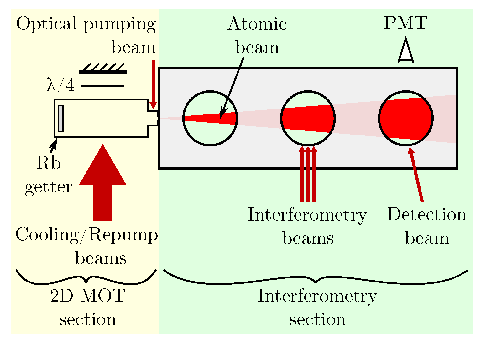
The beam apparatus consists of a rubidium-based 2D-MOT [22,25,26] connected to a science chamber machined from a rectangular prism (see Figure 1). The chamber, a stainless steel cell, 21.5 cm long, 7 cm tall, and 7 cm wide, is held at ultrahigh vacuum pressures (typically, 1–2 Torr) by an ion pump (not depicted in Figure 1) connected to the chamber approximately 26 cm away (as measured from center of atomic beam to center of the pump). The chamber also consists of eleven 2.75" ConFlatTM flange viewports, 3 to a side, except on the bottom. The 2D-MOT chamber is differentially pumped through a channel approximately m in diameter and 1 mm long.
2.1. 2D-MOT
The optics for the 2D-MOT chamber follow the standard design of counter-propagating circularly polarized light fields with the appropriate magnetic field generated by four permanent magnets. Light from the cooling and repump lasers are delivered to a cage assembly that houses 1 inch optics. As a result, the laser fields are circular and have a diameter of roughly inches. The diameter of the laser field matches the height of the 2D-MOT chamber (depicted in the left side of Figure 1) but is small with respect to its length. As a result, about one-third of the chamber is not exposed to the cooling beam. This choice was made on the basis of convenience in the optical design (i.e., no cylindrical lenses are required) and has the expected impact of a lower atom flux and slower atoms than an MOT with better optical overlap between the cell windows and the laser beam profile. Future designs will utilize better spatial overlap with the 2D-MOT chamber.
Cooling laser light is delivered to the cage assembly via single-mode polarization maintaining fiber. A combination of half-wave plate and polarizing beam splitter separates the light into a beam that eventually enters the chamber vertically and a second that enters the chamber horizontally. Light in the vertical direction is circularly polarized by a quarter-wave plate, sent into the chamber, and retro-reflected back into the chamber after passing through a second quarter-wave plate. The beam that enters the chamber horizontally is first combined with light that is delivered from the repump laser also via a single-mode polarization-maintaining fiber. The combined beams are then circularly polarized, sent into the chamber, and retro-reflected after passing through a second quarter-wave plate.
Located between the aperture of the 2D-MOT chamber and the science chamber is a clear glass-to-metal seal where the optical pump light enters the apparatus. While the glass allows us to insert a laser field for optical pumping (see Section 3), the surface flatness and uniformity were far too poor to allow for any kind of transverse cooling (i.e., using laser fields to better collimate the atoms emerging from the 2D-MOT). The cooling and repump beams were kept as close to the aperture as possible to allow the atoms to interact with the cooling beams for as long a time as possible before entering the science chamber.
The design of our atom source resulted in a beam of atoms with fairly high divergence traveling along the central axis of the science chamber (or interferometry section), as depicted in Figure 1. The specifics and consequences of this design have been discussed in detail in our previous work [27,28] and in the next section, we only briefly discuss the salient points.
2.2. Atomic Beam
2.2.1. Atom Signal Measurements
In order to characterize the atom flux as a function of cooling and repump laser power, a third laser, hereafter referred to as the “detection” laser, was directed into the science chamber. Of note, measuring the absolute atom flux was not necessary for our experiments; we used detection laser fluorescence as a proxy as it was simpler to measure and still allowed for meaningful characterization. As discussed in Section 2.2.3, the atom beam has a fairly large divergence. The divergence in both directions transverse to the direction of the atomic motion and the resulting uncertainty in the collection optics efficiency, coupled with optical pumping along the detection beam, make the absolute measurement of the atomic flux challenging and since absolute flux is not necessary for our experiments, we did not measure the absolute flux.
The relative atomic flux was measured as a function of the cooling and repump powers. Since the results mimic very closely the number of atoms captured in a 3D-MOT as the physics of the processes are every similar, we report these results in Appendix A. We checked the stability of the fluorescence signal by scanning the detection laser over the atomic resonance repeatedly once every 10 s for a 24-h period and plotting the Allan deviation of the measured atomic flux. Admittedly, this method is sensitive to factors not related to the atomic beam, such as detection laser intensity and electronic gain stability. Nevertheless, we found our system demonstrated approximately 15 min of stability before the signal started to drift, as measured by the Allan deviation. Further work will improve on the system stability.
2.2.2. Atom Beam Longitudinal Velocity
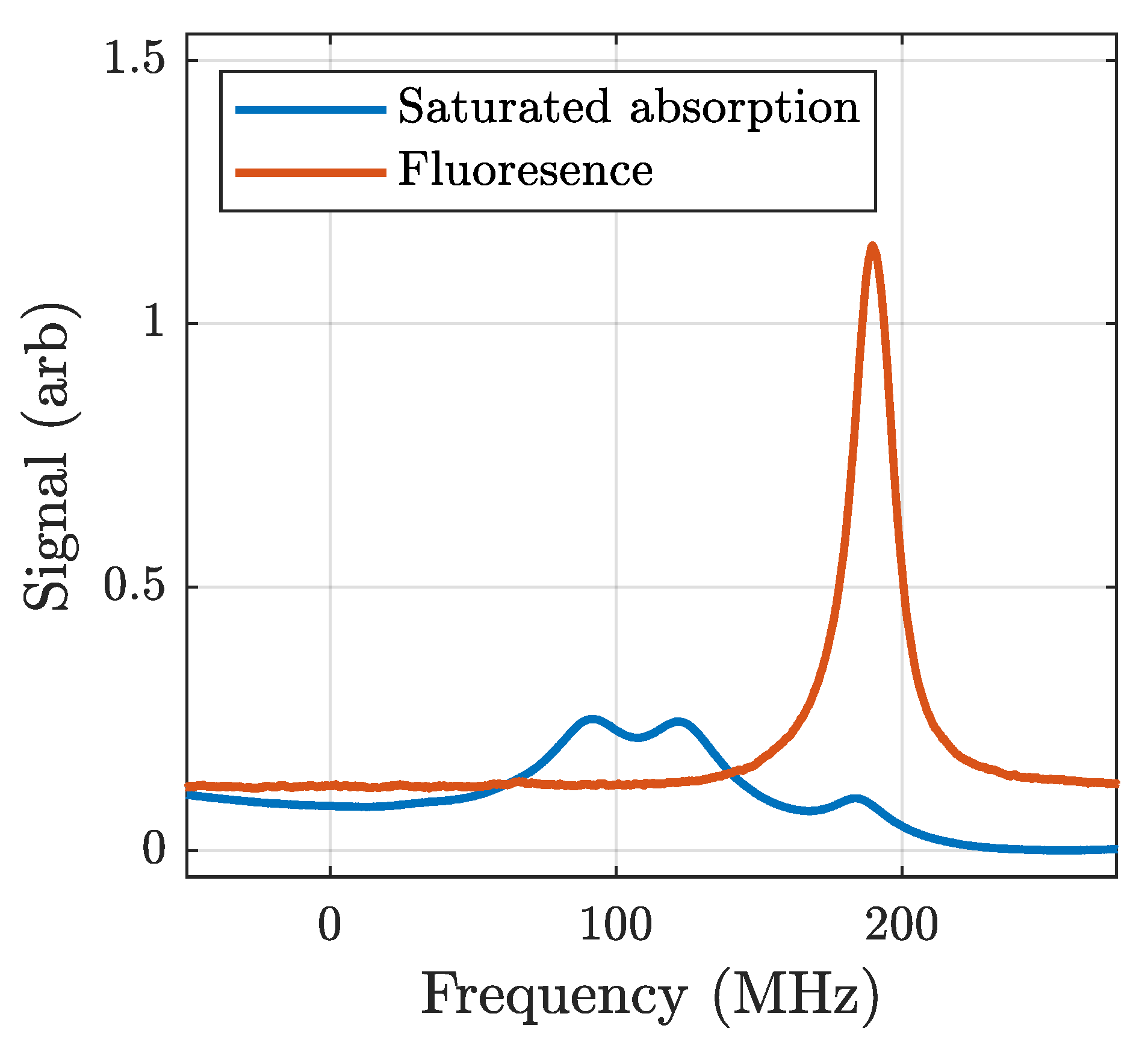
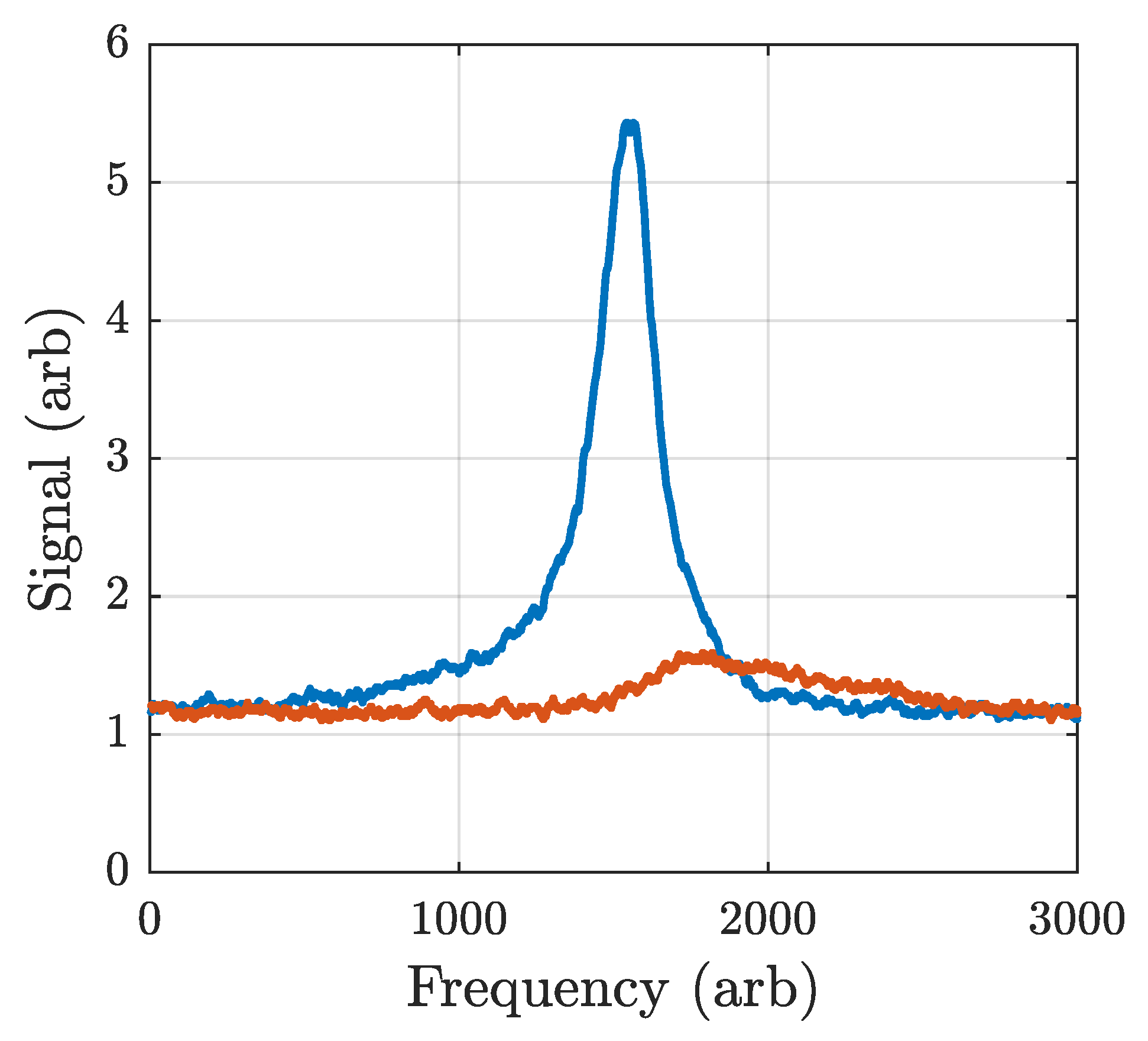
The atomic beam fluorescence measurements described in Section 2.2.1 were performed with a detection laser that was nominally orthogonal to the atom beam. It was oriented this way to avoid any Doppler shift or broadening of the spectrum of fluorescent light by velocity components of the atomic motion along the laser beam direction. However, we can intentionally orient the detection laser longitudinally and anti-parallel to the atomic motion to detect a Doppler-modified fluorescence spectrum and extract a velocity profile. The frequency of the peak is not exactly coincident with the -to- transition but rather Doppler-shifted proportionally to the speed of the atoms. The peak is not only Doppler-shifted, but the spectral width is also slightly broadened because the beam is not monoenergetic and instead contains a continuum of velocity classes. Since the vacuum chamber was designed to have two atomic sources, one at each end of the science chamber, there were two pinholes (apertures) conveniently placed that we used as alignment holes. We aligned a scanning detection laser through these holes and collected the fluorescence induced by the laser. We compared the data to a saturated absorption trace taken simultaneously, which enabled us to properly define the “zero” frequency shift. We measured the frequency difference between the fluorescence peak and the transition in the saturated absorption spectrum. The two traces are shown in Figure 2 and the frequency shift is highlighted. If we assume the shift is dominated by atoms in , the most probable velocity group, then this shift corresponds to m/s. Systematic effects in the frequency calibration dominated errors in this measurement, and accuracy was limited to a velocity range corresponding to a Doppler shift on the order of the natural linewidth of the transition ; , where is the wavelength of the transition. Frequency-dependent optical pumping along the detection beam path (which overlapped the atomic beam path for this measurement) could likewise cause changes in lineshape and additional systematic errors. Given that our expected errors are comparable to our measured value, we also explored an alternative, time-of-flight-based technique to obtain a more accurate value.
We found that the optical pumping scheme (described in detail in Section 3) could be used as a “switch” for the atom beam. The optical pumping beam was derived from the cooling laser and double-passed through an acousto-optic modulator (AOM), without blocking the zero-order component as is usually done. The zeroth-order beam had no frequency shift relative to the cooling beam and the first-order beam had a frequency shift that was twice the frequency driving the AOM. Both beams were sent to the optical pumping port of the interferometer. When the signal to the AOM driver was off, the optical pumping beam was nearly resonant with the transition, which is quasi-closed. This transition can scatter thousands of photons before the atom is optically pumped into the dark state. Since momentum is conserved, the atom beam is deflected by the optical pumping beam and does not pass through the aperture. The radio frequency driving the AOM was chosen such that when signal was on, the twice-frequency shifted light was on resonance with the transition, which on average requires only a couple of photons to optically pump into the dark state. Importantly, this optical pumping still occurs even in the presence of non-negligible zeroth-order light that is still resonant with the transition. In that case, a beam of atoms optically pumped into the proper state () propagates down the vacuum chamber. This feature lends itself well to another velocity profile measurement of the atom beam (to compare with the measurements described in the preceding paragraph). By rapidly switching between the two configurations, we can create a pulsed beam of atoms and can use time-of-flight methods to measure the velocity of the atoms.
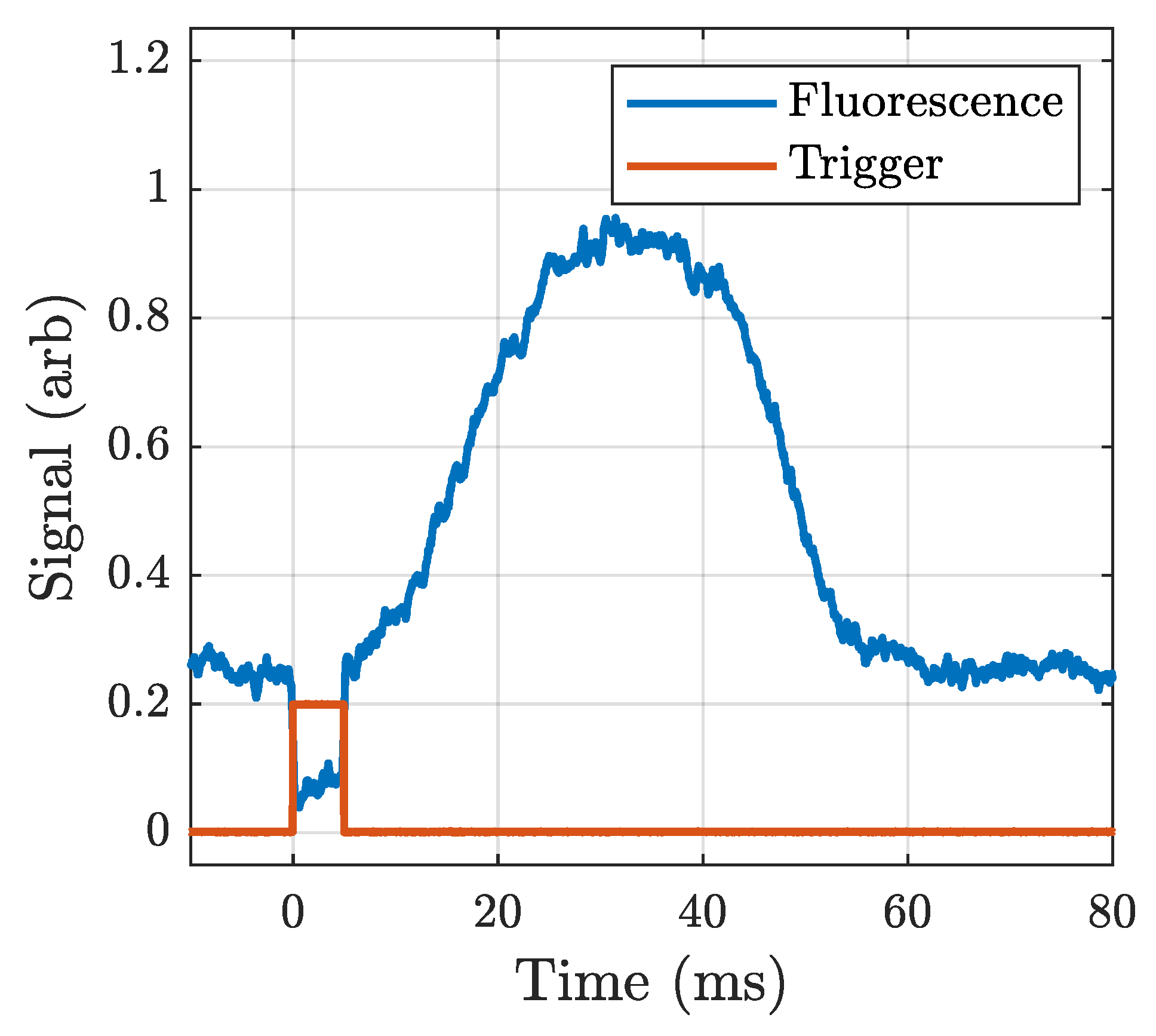
Our time-of-flight method started with a detection laser locked precisely on the transition. The AOM driving frequency was initially configured so that the optical pumping light was on-resonance with the transition and therefore, the atomic beam is deflected and the atoms were blocked by the aperture. We introduced a brief step function that produced a pulse of atoms making it through the aperture in the dark state which were subsequently repumped into the bright state for detection. Figure 3 depicts the result. The atomic beam was pulsed on at time ms for 5 ms. We see depicted a baseline of no signal increasing to a peak before falling away again. This signal represents a packet of atoms propagating down the vacuum chamber. The width of the peak is a consequence of the velocity spread of the atoms and the center of the peak gives the most probable velocity of the atoms. The known distance divided by the measured time resulted in an extracted velocity of m/s, consistent with our earlier measurement of ∼4 m/s, given the large errors associated with that measurement.
2.2.3. Atom Beam Divergence
The atom beam divergence measurement is discussed in detail in [27,28] so we briefly summarize the procedure here. In order to measure the atomic beam divergence, we imaged fluorescence from the vacuum windows at two points, measured the fluorescence profile, and extracted the divergence from those measurements. The detection beam was locked on-resonance and directed into the vacuum center from above at the first window (see Figure 1). The laser beam was circular and had a diameter of about 1 mm. The fluorescence from the atoms at the intersection of the atomic beam and laser beam was imaged onto a camera and recorded using an imaging system with a pre-calibrated magnification factor. This process was repeated with the detection laser beam moved to the second window, which was at a center-to-center distance of 7.4 cm. We numerically fit the intensity of the fluorescence images to a Gaussian function and extracted from each measurement a value. We find an atom beam (half-angle) divergence of 56 mrad. This value is consistent with a preliminary measurement we made using the same approach but between two points within one window. Unfortunately, due to geometrical constraints, we could not apply any focusing techniques to the atoms as they exited the 2D-MOT chamber into the science chamber. The large divergence negatively impacted our results in two ways.
Firstly, as the atoms were traveling at an angle with respect to any laser beams entering the chamber, the length of time the atoms spent in the laser beam is not uniform for all atoms. The “pulse” of light experienced by the atoms was a function of the angle at which the atoms were emitted from the aperture and their velocity. Secondly, the length of time the atoms spent in the dark is similarly a function of emission angle and velocity.
In addition to the divergence of our atomic beam, our optical beams also had divergence. Both divergences ultimately led to a loss of contrast in measurements were primarily due to velocity averaging; we confirmed this in detail with modeling [27,28]. Minimizing atom beam divergence is less critical than minimizing the laser beam divergence, but is also less easily done.
One additional effect not considered in this experiment, but one that will be relevant for future experiments, is the divergence along the direction of the Raman beams, which were orthogonal to the detection and atomic beams. In the experiments reported in this paper, we used co-propagating Raman beams, which are Doppler-insensitive (meaning they are on two-photon resonance regardless of the velocity of the atoms). For experiments that involve counter-propagating Raman beams that are Doppler-sensitive, large divergence will mean that only certain classes of atoms with the right transverse velocity will be on-resonance.
3. Optical Pumping as a Switch
In Section 2.2.2, we discussed the fact that using the to transition to optically pump atoms into the state caused the atoms in the atomic beam to be deflected. We performed a series of experiments to confirm the deflection of the atom beam and to confirm the effectiveness of as an optical pumping pathway.
A typical experiment to measure the number of atoms in the detection region uses a laser (the “detection laser”), which scans over the transition. As the detection laser is strong (in the Rabi sense), optical pumping usually occurs quickly and only the transition is detected. As a result, the fluorescence from the atoms has a single Lorentzian profile. Introduction of the optical pump beam which is designed to pump all the atoms into the state can lead to a drop in the signal, ideally to zero if the drop is due to true and complete optical pumping. Unfortunately, a drop in signal can also be caused by a complete loss of atoms (from atom beam deflection, for example) rather than complete optical pumping.
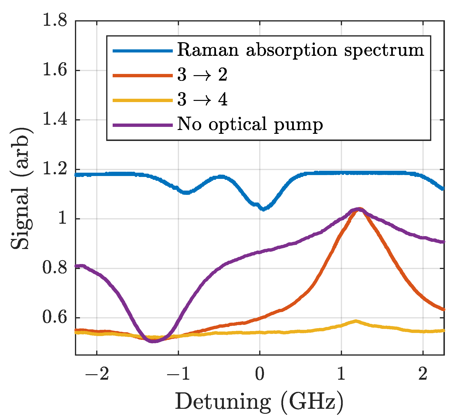
To unambiguously differentiate between good optical pumping and no atom beam, we performed the following experiment, the results of which are depicted in Figure 4. We locked the detection laser on the transition frequency and monitored the fluorescence from the detection region as we scanned the frequency of a single laser beam from an additional auxiliary laser that intersected the atomic beam upstream from the detection region. For convenience, we used the red-shifted beam from our Raman laser setup as this auxiliary laser.
Excited atoms can decay into different ground states as a result of selection rules; the ratio of these paths is the branching ratio. It is calculated by summing dipole matrix elements for the transitions between the various magnetic sublevels [29,30]. For the purposes of this discussion, the units of these numbers may be considered arbitrary, and their utility comes from summing all of the elements for a given hyperfine transition (i.e., to F). We looked at decay from and into and .
From Figure 4, first consider the fluorescence trace with no optical pump (“No Optical Pump”, solid purple trace) relative to the absorption trace. Since there was no pumping, the atoms were in some combination of the and states as they entered the science chamber (numerical modeling indicates they are mostly in the state). As the atoms traveled down the chamber, they were first illuminated by the auxiliary laser as it scanned through the manifold, which optically pumped the atoms into the state, and then illuminated by the locked detection laser. Since the atoms were optically pumped by the auxiliary laser, they were not excited by the detection laser, resulting in the dip in the left side of the “No Optical Pump” trace. Atoms that were illuminated by the auxiliary laser as it scanned through the manifold were optically pumped into state and were excited by the detection laser, resulting in the peak on the right side of the “No Optical Pump” trace. (Note that the positions of these resonances are shifted by GHz relative to the manifold in the absorption trace for the reason described above.)
Next, we consider the traces with optical pumping on, starting with the yellow “” trace. We expected this light to displace the atom beam such that it is mostly deflected and therefore no atoms reach the detection laser, and that is exactly what we saw. Finally, with the pump on, all of the atoms were in as they entered the vacuum chamber. Atoms that were illuminated by the Raman laser as it scanned through resonance were put back into state and were excited by the detection laser, as seen by the peak on the right side of the “” trace. Atoms illuminated by any other frequency of light did not make it into the state. With this method, effective optical pumping will result in a baseline at the intensity of the “No Optical Pump” dip and a peak height at the intensity of the “No Optical Pump” peak, which is precisely what we measured here.
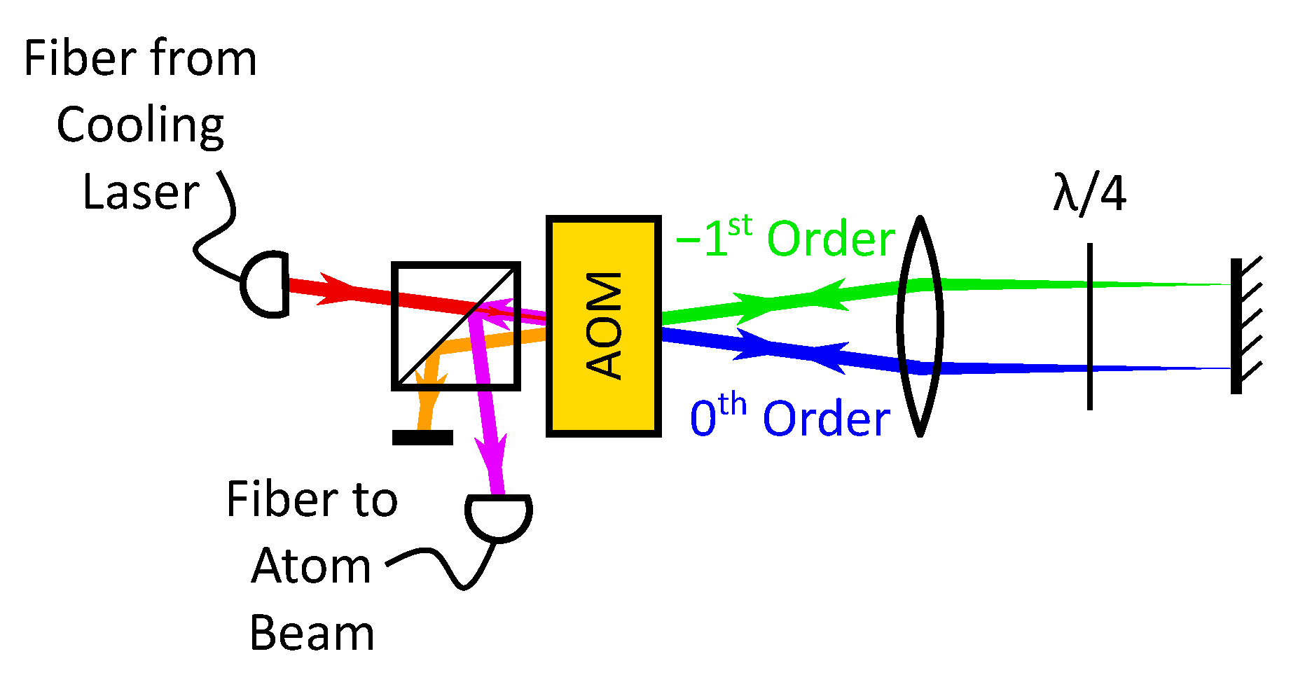
The optical setup used to create the light for optical pumping and atom beam switching was a variation of a standard double-pass AOM setup, and it is depicted in Figure 5. We started with light from our cooling laser, which was tuned ∼6 below the transition. On a first pass through the AOM, there were two primary output beams; the first was the -order beam that has picked up a negative frequency shift (equal to the AOM drive frequency ) and an angular deviation, and the second was the 0-order beam with no frequency or angular shift from the input. As with a normal double-pass setup, we arranged a lens at its focal length from the AOM to align these beams parallel to each other, allowing us to retroreflect both in a way that was insensitive to the angle/drive frequency. The retroreflection was also performed at one focal length from the lens, in the so-called cat’s eye configuration, which resulted in a collimated beam for a second pass through the AOM.
Similar to a normal double-pass AOM setup, this geometry naturally resulted in the retroreflected -order beam being at the correct angle to be frequency-shifted again in the same direction (in our case, negative), during the second pass. This beam also had an angular shift back onto the original input beam path (counter-propagating), and was shifted by relative to the input beam. To eliminate the spatial overlap with the input, a waveplate was used in the retroreflection arm, along with a polarizing beamsplitter cube on the input side of the AOM, to divert this output beam to be used in the experiment. As with the first pass, there was a portion of light that was unshifted during the second pass. This light was frequency-shifted by relative to the input beam due to the first pass, and was not spatially overlapped with the input. This unwanted beam was easily blocked and eliminated with an iris.
Unlike a normal double-pass AOM setup, we did not block the first-pass 0-order beam from making a second pass through the AOM. Instead, we retroreflected this beam as well, which was also naturally at the correct angle for a frequency shift from the AOM (of opposite sign, in this case, positive). This beam also created two outputs upon going through the AOM a second time. One of these picked up a frequency shift, this time in the opposite direction (for a total shift of relative to the input beam), and was spatially overlapped with our unwanted, blocked beam from the first-pass order. The other picked up no frequency or angular shift from either pass, it was at the input frequency, and it was spatially overlapped with our output beam of interest (as well as the input beam up until the beamsplitter). This beam was also present—and contained all of the output power—when the AOM was switched off.
The result of this arrangement was that we had two spatial modes being output from the second pass when the AOM was on. One of these contained two frequencies of light we did not have a use for, and this was blocked. The other was coupled into a single PM fiber and directed into the optical pumping region of the experiment. This single spatial mode contained both light that was near the transition frequency, and light that was frequency shifted by relative to this. The drive frequency was chosen such that this frequency was on resonance with the transition for efficient optical pumping. Since the optical pumping for this transition was significantly faster than for the transition, the atoms were pumped to the dark state by the “correct” light before the “incorrect” light had a chance to give the atoms a momentum kick, so we were left with a beam of atoms in the ground state. When the AOM was off, all of the light was output at the transition frequency, and driving this closed transition resulted in a significant momentum kick to the atoms, which caused the atomic beam to miss the aperture, effectively turning it off.
4. Detection Apparatus
4.1. Detection Laser Shaping
In this section, we briefly describe some additional considerations for designing the beam shaping optics for the detection beam. In the upcoming sections, we specifically concentrate on the longitudinal and transverse dimensions of the laser beam and the laser beam’s incident angle.
4.1.1. Longitudinal Width
Here, we describe the procedure we used to determine the proper longitudinal spatial extent of the detection laser field. In principle, the task of collecting fluorescence from an exciting laser beam is straightforward: illuminate the atoms with an on-resonance laser field, collect the fluorescence with a lens, and focus the light onto a photo-multiplier tube or other sensitive optical detector. By knowing the detection geometry and hence the geometric collection efficiency and fundamental atomic parameters such as the spontaneous decay rate, one can, in principle, extract the number of atoms in the excitation region. This procedure has worked well in other atomic beam experiments, e.g., [15,31,32,33]. In those and similar experiments, the atomic beam was well-collimated and hence, the interaction region was fairly small (∼1 mm), so that a paraxial approximation for the light collection would be suitable. Additionally, the longitudinal velocity was sufficiently high that most of the atoms did not have time to be optically pumped into the dark state (especially since the combination of an applied magnetic field and a circularly polarized detection field leads to a closed transition). For our experiment, the open nature of the transition coupled with the low velocity of the atoms means that optical pumping needs to be taken into account.
The ground states in Rb have total angular momentum and , and the excited states of the D2 transition have total angular momentum , which results in 36 magnetically sensitive energy levels, as shown in [29]. We developed a simple rate equation model that accounts for the population in all 36 levels, allowing for differing coupling strengths [29] and different polarization states for a laser field tuned close to the transition. Using this model, we explored the length of time it takes for atoms to optically pump into the dark state, and we found that in all cases under strong pumping, the atomic population decays exponentially from the to ground state with a 1/e time that is dependent on the laser intensity. For our value of the available laser power, the 1/e time was about 10,000 times the excited state lifetime for the Rubidium D2 line. The atoms will “go dark” after traveling for a time of ∼270 s, which corresponds to a distance of ∼1.6 mm based on the mean velocity of the atoms (see Section 2.2.2) of 6 m/s. We performed a rough check of these calculations by introducing a rectangular slit into the detection laser to produce a beam that is about 2 mm in the transverse direction and variable in the atomic beam longitudinal direction. As atoms get optically pumped, they turn dark and so a longer beam in the longitudinal direction will only produce more background scattering and no more atomic scattering. By scanning the frequency of the detection beam and monitoring both the signal-above-background as well as the absolute background signal and varying the slit width, we found the optimal longitudinal width of the detection beam to be about 2 mm. Subsequent designs for the detection laser included beam shaping optics that resulted in a beam with longitudinal extent of approximately 2 mm.
4.1.2. Transverse Width
As mentioned, our atomic beam has a broad transverse velocity distribution. Due to the Doppler-free aspect of our current laser beam configuration, this transverse velocity contributes little in the measurements we performed apart from transit broadening and non-uniform time the atoms spend in the light fields in our Raman and Ramset experiments. Therefore, it is advantageous to have a detection beam that is large enough to excite all the atoms in the atomic beam yet no larger, to avoid introducing unnecessary scattered light from the windows, vacuum system, etc. By optimizing the signal-over-background as we did in the preceding section, but this time varying the width in the transverse direction, we found the optimal width in the transverse direction to be ∼2.6 cm.
While this configuration maximized the signal-over-background for the Doppler-free configuration, it will not be optimal for the future Doppler-sensitive experiments that we have planned. When switching to the Doppler-sensitive configuration, we can restrict the size of the detection laser beam so that we only detect the atoms within a given (smaller) divergence angle. This reduction will have the effect of reducing the Doppler width of the Raman resonance in the Doppler-sensitive configuration, at the expense of signal-above-background. Reduction of the height of the Raman beam in the orthogonal direction will also have a similar effect. The expected Doppler broadening for atoms with a mean velocity of 6 m/s and a half-angle divergence of 56 mrad in the Doppler-sensitive configuration is about 430 kHz, which needs to be compared to the expected Raman linewidth in our system. For an atom traveling with a velocity of 6 m/s and assuming a 1 mm diameter beam for the Raman fields, beam, then roughly speaking, the 1/transit time frequency is 6 kHz. Thus, we would expect a Raman spectral width of about 430 kHz if all the atoms participated in the Raman process.
4.1.3. Incident Angle
When the system parameters—namely, cooling laser power and detuning, repump power and detuning, and rubidium dispenser current—were optimized for the maximum flux, we found that the collected fluorescence from a scanning detection laser (nominally at right angles to the axis of the atomic beam) consisted of a large, narrow peak as well as a smaller, broader peak. The broader peak remained when the cooling or repump laser was blocked. Traces for the fluorescence with and without the cooling laser on are shown in Figure 6. We interpreted this broader peak to be “hot” (thermal) atoms escaping through the pinhole. The width of the broad peak was not consistent with a room-temperature Doppler profile, likely caused by velocity selection due to the geometry of the design. In order to avoid collecting fluorescence from hot atoms, we relied on the relatively low velocity of the cooled atoms. We sent the detection laser beam into the chamber at as steep an angle as the ∼1.5” clear aperture window would allow (∼). This caused the peak of the Doppler-broadened line to shift relative to the uncooled peak enough to spectrally resolve the line-shapes. Furthermore, as outlined below in Section 4.2, we dithered the detection laser frequency on the side of resonance for a lock-in detection technique. When we did so, we always set the central laser frequency to the low side of the resonances, further eliminating contamination of the signal from the unwanted fluorescence from the hot atoms.
4.2. Lock-In Detection
Since all the laser beams used in this experiment are on continuously, a lot of stray scattered light reaches the detector. As a result, the fluorescence from the atoms in the state can be small relative to the background signal caused by this scattered light. In this section, we describe our method for using a lock-in amplifier to reduce the background signal while amplifying the signal. Since the parameters we are scanning for experiments (optical pumping or Raman frequencies) are not the same as the dithered parameter (detection laser frequency), this technique directly recovers the signal of interest and not the derivative-like signals that result from other lock-in techniques. Below, we describe this method to measure the Raman spectrum from the atoms. The same method is used for measuring Ramsey interference as well.
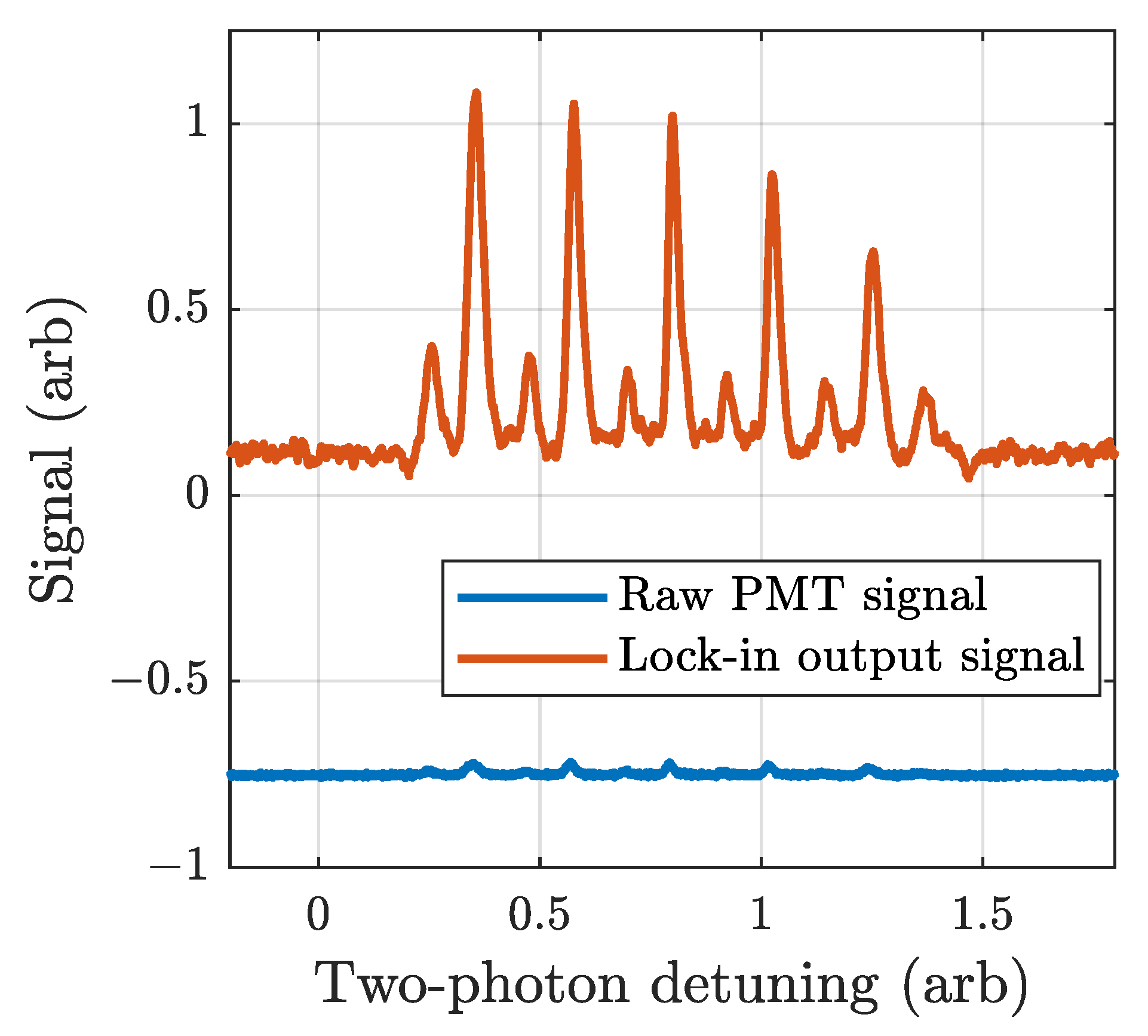
The lower blue trace in Figure 7 shows the result of a Raman spectrum measurement, as measured directly with the PMT. The measurement consisted of atoms emerging from the 2D-MOT source and being optically pumped into the ground state. The atoms passed through a single spatial mode of a laser field that consists of two frequencies nominally separated by the ground state splitting. The intensity of the laser fields and the spatial width of the laser fields were chosen to maximize the Raman peak of the clock transition. The atoms then traveled to the detection beam. The detection beam was shaped as described in Section 4.1. For normal operation of a lock-in amplifier, one might “chop” the detection laser (i.e., cycle the amplitude) and lock-in detect on the chopping frequency. However, as the scattering is partly caused by the detection laser itself, the detection laser scattering would also be amplified by the lock-in amplifier. Another normal mode of operation for the lock-in amplifier is to dither the frequency of the detection laser and lock-in detect on the dither frequency to create a line shape that is a derivative of a Lorentzian. We indeed dithered the detection laser frequency, but since this is not the parameter we are scanning in the experiment (which in this case is the two-photon detuning of the Raman fields), it resulted in a direct copy of the Raman signal (amplified and without the background) rather than a derivative. The detection laser was nominally locked to the low-frequency side of the peak of the transition. By frequency-modulating the detection laser, the fluorescence was amplitude-modulated but the background light was not amplitude-modulated (to first order). This enabled us to run the lock-in amplifier with an amplitude-modulated signal. Of course, there was additional (strong) background light from the Raman laser that reached the PMT as well. This light was not affected by the dithering of the frequency of the lock-in amplifier and so it was also filtered by the lock-in amplifier. Figure 7 (the upper red trace) shows the result of a measurement of the Raman signal under the same conditions as those for the blue trace, but using the lock-in amplifier.
However, one drawback of using the lock-in amplifier in this manner is that the bandwidth of the entire measurement system decreases substantially. As is well known, the linewidth of a Raman transition is inversely proportional to the time the atoms are exposed to the Raman field. In our case, this time is effectively set by the transit time of the atoms through the Raman laser beam. We used a laser beam spatial width of approximately 2 mm and the most probable velocity of our atoms was measured to be m/s. Therefore, the transit time was 300 s (corresponding to a linewidth of 3 kHz). To avoid measurement broadening, the sweep rate of the Raman laser needs to be kept below 3 kHz/s. The full Raman spectrum consists of 11 peaks [34,35] whose entire frequency span depends on the applied magnetic field strength. Taking the component of the Earth’s magnetic field along the direction of propagation of the Raman field to be of the order of ∼0.1 Gauss (controllable by coils in our system) and noting that the transitions in Rb have a first-order Zeeman shift of 1 MHz/Gauss, the full Raman spectrum spans MHz. Thus, the total scan time cannot be faster than s. To obtain a decent lock-in amplifier signal, one needs to integrate for at least 100 cycles of the modulation frequency (and 1000 is better). Making a trade-off between data collection time and minimizing measurement broadening, our typical sweeps time of the Raman laser across the entire Raman spectrum lasted 10 s, although we used faster scan times for scans with lower amplitude.
5. Raman Laser
5.1. Construction
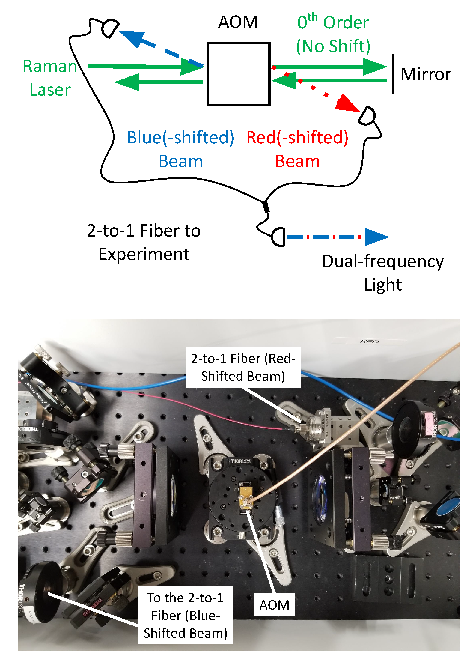
Both of our frequency-shifted Raman beams were derived from the same laser source (a distributed feedback laser or DFB). The overall frequency stability requirement is not as stringent as that of the other lasers. The cooling, repump, and detection lasers need to be stabilized to much less than a natural linewidth, which in rubidium is MHz. On the other hand, the Raman laser is typically detuned by several hundred MHz, so drifts in the order of 1 MHz are insignificant to the first order in our experiments. This alleviated the need for a saturated absorption setup and allowed for a simpler single-pass absorption cell setup to be used to monitor and tune the laser. The optics scheme for the light that goes to the experiment is depicted in Figure 8 (top) and a photo of the setup is shown in Figure 8 (bottom). The beam was oriented in a double single-pass configuration through an AOM (in this case a Brimrose GPF-1500-780 driven by an Analog Devices AD9914 3.5 GSPS direct digital synthesizer (DSS) and RF amplifier). A single pass produces a beam (1st order) that exits at an angle with a frequency shift equal to the RF drive frequency, carrying ∼20% of the incident light. The unshifted beam carries the remaining 80% of the power. By retroreflecting this 0th-order beam one can produce an additional 1st order beam traveling in the opposite direction, with a frequency shift of the same magnitude but opposite sign as the first-pass 1st-order beam. When the angle of the AOM and the incident laser are optimized for efficient generation of the first-pass 1st, the angle of the AOM is automatically phase-matched to a produce the second 1st-order beam. The result of this double single-pass configuration produced two spatially distinct laser beams (whose polarization can be independently adjusted with waveplates as needed) and whose frequency difference is set by twice the RF frequency driving the AOM with a frequency stability of about 10 Hz (limited by our reference source). These two beams were then combined via a two-to-one PM fiber into a single physical beam of laser light. The two beams of light emerging from the fiber nominally had linear polarization.
5.2. Masks
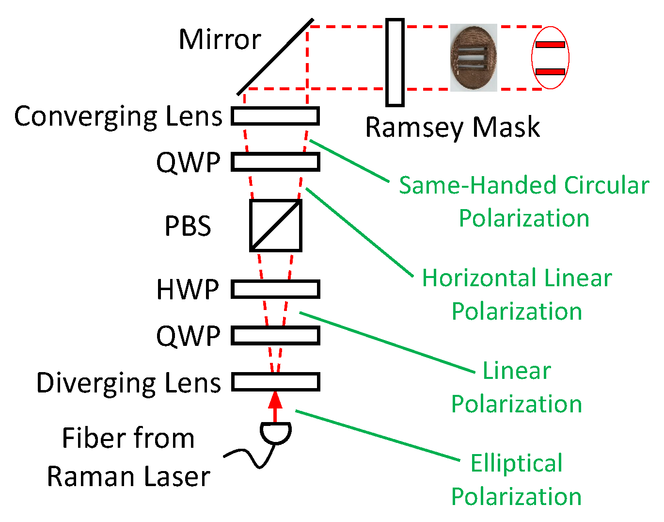
To create the individual beams necessary for interference experiments, we utilized a mask to create nominally identical physical beams from a single large Raman beam. Figure 9 depicts the optics used in this method. A combination of diverging and converging lenses was used to create a single, large, collimated beam. Ideally, they would be placed in a collimated beam rather than a diverging one; however, the placement was necessary due to physical limitations of the optics breadboard. The first QWP is a “fixer” used to turn the elliptically polarized light emanating from the (imperfect) PM fiber into completely linearly polarized light; the second quarter waveplate was used to ensure the same handedness of circular polarization. The half waveplate and PBS are used as a controllable power attenuator. Figure 9 depicts a spin echo mask as an example, but we have a variety of 3D-printed masks with one, two, and three slits for Raman, Ramsey, and spin echo spectra, respectively.
However, the mask method does have some characteristics which are not desirable. Since the mask size is comparable to the size of the laser beam’s Airy disc, the relative intensity of beams near the edges is dependent on precise placement of the mask with regards to the center of the disc. Similarly, the intensity of the beams is dependent on the slit spacing of the mask (the greater the separation of the beams, the weaker their intensity). These disadvantages do not come into play for the central, single-slit Raman configuration, but they are a factor for Ramsey interference and will be for spin echo interference. Finally, there is the fundamental presence of optical diffraction as the light passes through the slits. We projected the beam across the lab to look for diffraction effects in the far field. Diffraction was strongly present when the slits were ∼1 mm wide, but not noticeable when the slits were 2 mm wide (which became our normal operating slit width).
One final drawback of the mask method is that it caused power to be “thrown away”. The power coming out of the fiber is spread out over a large surface area, resulting in low intensity, forcing us to include a tapered amplifier (another Thorlabs TPA780P20 Tapered Amplifier mounted on a Thorlabs LDC2500B Tapered Amplifier Controller) when using the mask method. For typical operating power levels, we found the performance to be adequate, with the extra power (and signal) gained being worth the addition of unwanted on-resonant amplified stimulated emission (ASE). In addition to providing increased power, the inclusion of the amplifier also allows for easy adjustment of the power level, which is useful for characterization.
5.3. Optimization of the Raman Beams
5.3.1. Elimination of the AC Stark Shift
We were able to characterize the experimental apparatus and measure a multitude of relevant parameters. We began by minimizing the AC Stark shift. The AC Stark shift is proportional to (where is the zero-detuning single-photon Rabi frequency of the i- transition) and inversely proportional to the single-photon detuning. (For large detuning, the average single-photon detuning of the two Raman fields can replace the individual single-photon detuning in the expression for the AC Stark shift.) We arbitrarily chose a value for the single-photon detuning that was close to resonance yet not so close that the coherent Raman process was masked by incoherent scattering. We measured the clock transition frequency at multiple total beam powers for a given power ratio of the blue- and red-shifted beams. If it shifted for different total powers, different combinations of filters were placed in front of the red and blue Raman beams to produce a different power ratio. The process was iterated until no frequency shift was measured. This iterative process resulted in a red-to-blue beam power ratio of 2.3:1.
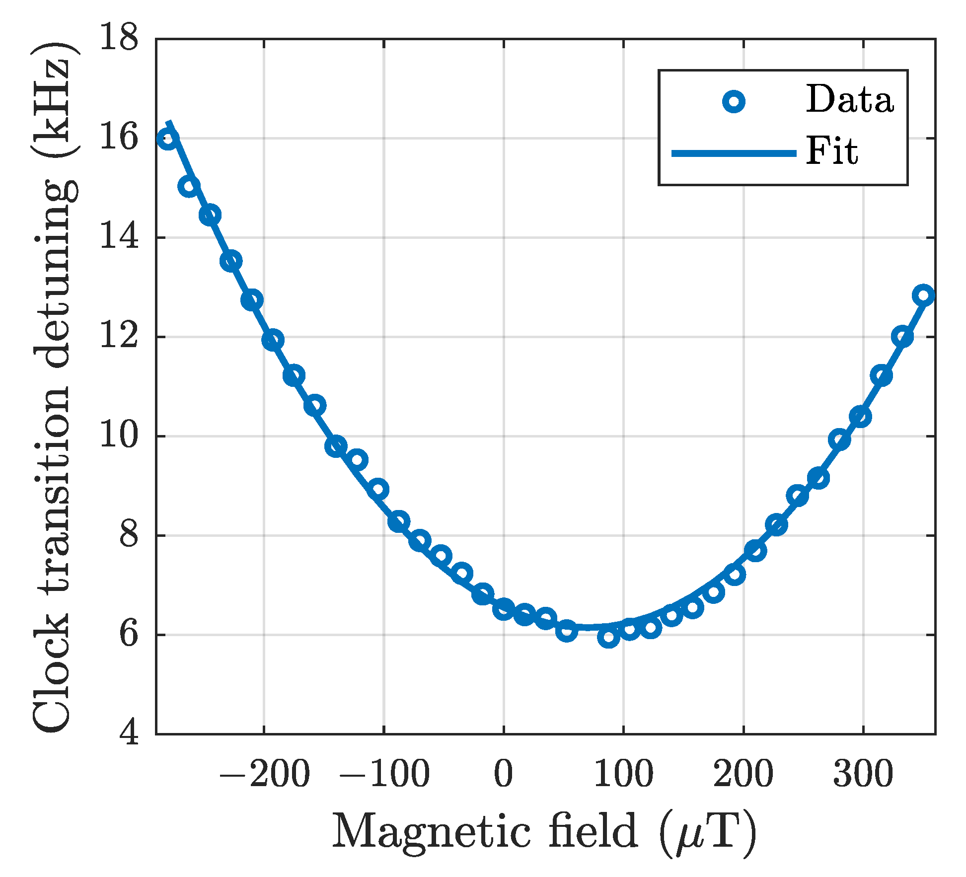
5.3.2. Magnetic Field Measurement
We used the Raman transition to measure and manage the magnetic field in the vacuum chamber with electromagnetic coils [34,35] which were included for two reasons. The first is to spectrally isolate the clock transition. A magnetic field (with the appropriate strength) applied along the direction of propagation of the Raman laser beam(s) frequency shifts the other 10 Raman transitions farther away from the central clock transition [35]. The second reason is to minimize second-order Zeeman effects. Figure 10 depicts the clock transition peak position as a function of the applied magnetic field (in the direction of the Raman beams).
5.3.3. Setting the Condition
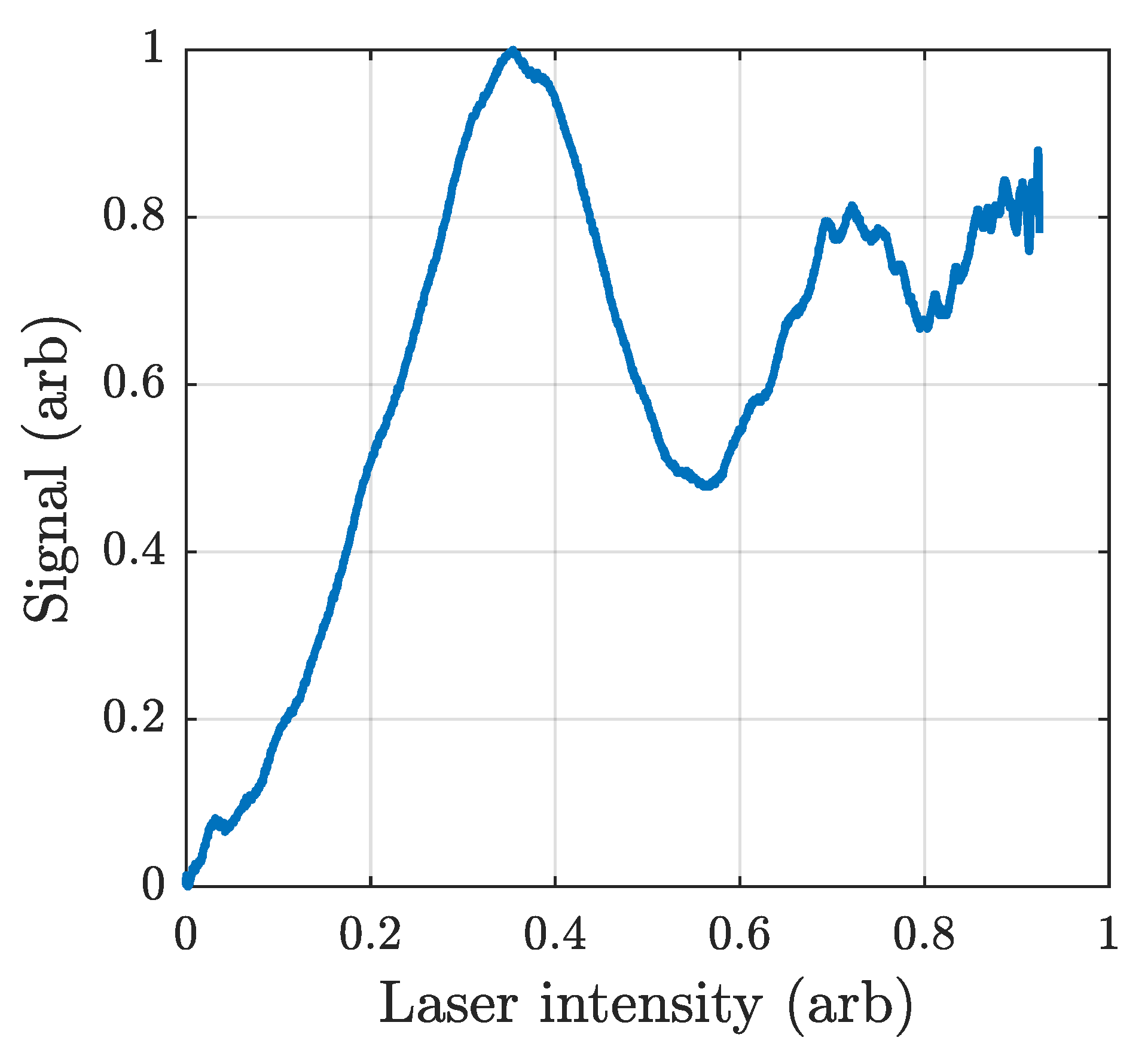
We evaluated the signal above background as a function of total Raman beam power by adjusting the current in the tapered amplifier. We expect the signal to increase up to a point before falling off again—this maximum is the -pulse condition. We set the magnetic field to a value that spectrally resolved the clock transition. We then scanned the Raman laser frequency over the clock transition frequency and recorded the amplitude of the resultant scan for a range of total Raman powers. This method has the advantage of not needing additional equipment, but the disadvantage of being both discrete in laser power and time-consuming. We performed a similar measurement in which we kept the two-photon Raman frequency fixed and scanned the Raman laser power. We added a low-frequency AOM, passed the Raman fields through it, then sent the 1st-order beam to the vacuum chamber. The scan of the optical power was not linear but this was accounted for by “picking off” a portion of the laser beam and monitoring the power with a photo-detector. The results of these measurements are plotted in Figure 11, they are similar to the modeling discussed in [36], and they show Rabi oscillations as the laser power increases above the -pulse condition. The dephasing is likely caused by three effects. As the power increases, so do any residual AC Stark shifts, although we minimized the shifts as much as possible. The changing AC Start shift will appear as an increased detuning for the higher power, causing a drop in the oscillation amplitude. Secondly, the effects of incoherent scattering caused by the fact that the Raman fields are not “infinitely” single-photon detuned increase with increasing power. Finally, the atomic beam is not mono-energetic: the atoms have differing speeds which translates to differing times in the atomic beam and thus, the measurement is an average over all possible velocity classes/transit times.
6. Representative Data
In this section, we present some representative data collected from our apparatus. The main goal of these experiments was to produce Raman spectra with as large a signal-to-noise ratio as possible and demonstrate that we could also observe Ramsey interference despite velocity and transit time averaging.
6.1. Doppler-Free Raman Spectroscopy
Having optimized the parameters of our system, we turn to the presentation of typical data. The magnetic field coil was turned off so that the magnetic field around the atoms would be carbitrarily oriented with respect to the propagation direction of the Raman fields. This results in an 11 peaked spectrum [34,35]. Such a spectrum was depicted earlier in Figure 7. We used a red-to-blue power ratio of 2.3 to eliminate power-dependent AC Stark shifts (empirically determined), with the polarizations of the red and blue constituent beams matched (parallel linear). A downstream quarter-wave plate changes the linear polarization to same-handed circular polarization.
Total beam power was low (typically less than 5 mW as measured prior to the atom beam) due to sequential losses in the optics setup. Additional power will not appreciably help the signal in the Doppler-free configuration as we are already operating in the -condition. However, due to the fairly wide transverse velocity of the atomic beam, additional power may be required when the apparatus is placed in the Doppler-sensitive configuration. By carefully selecting the output parameters of our RF source, we were able to measure all 11 Raman peaks in the arbitrary magnetic field present in our lab. A combination of the magnetic sublevels of each manifold combined with selection rules results in 11 magnetically sensitive “paths”. We added magnetic coils as well, which allowed us to drive only the six even or five odd peaks as desired by adjusting the current through the coils (and thus, the direction of the magnetic field; this technique is described in detail in [35]. We have typically adjusted the current such that the even peaks are prominent as these contain the zero (or clock transition) peak, which we will use for Ramsey interference. A typical trace of a clock transition measurement is depicted in Figure 12.
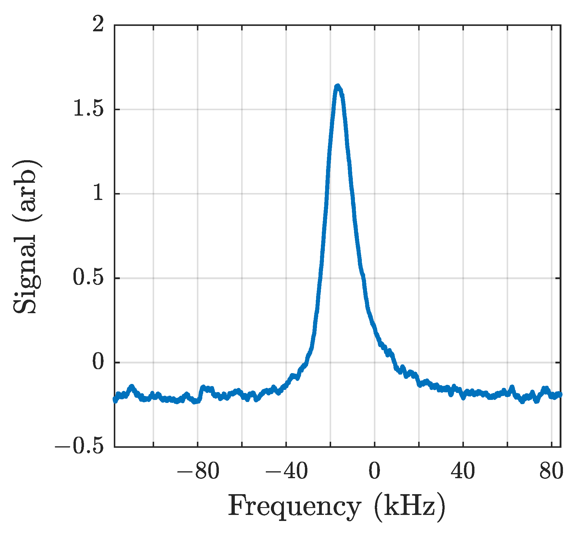
6.2. Doppler-Free Ramsey Spectroscopy
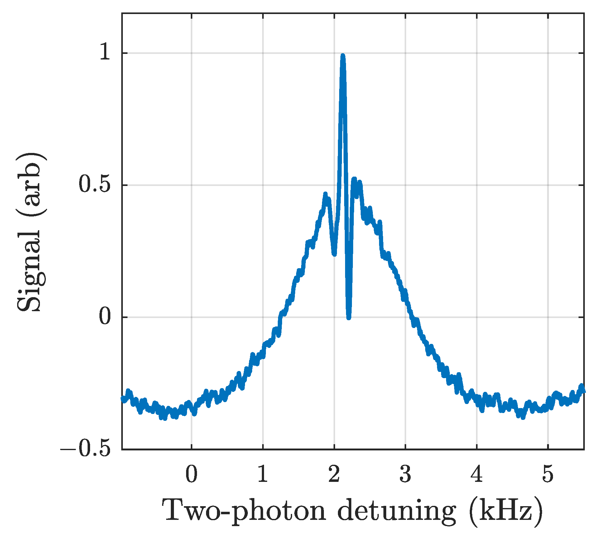
As shown in [37,38], Ramsey interference is a result of a pulse sequence. This is a useful intermediate step (en route to a full interferometer) as it represents the simplest form of atomic interference we can generate in the experiment. More importantly, it was crucial in that it demanded that all of our Raman settings were correct. We can only see it if the physical beams have acceptable coherence, geometry, and are truly providing the atoms with -pulses (up to Doppler averaging). Figure 13 shows a representative trace of an optimized Doppler-free Ramsey interference pattern and is one of the main results of this paper—the demonstration of Doppler-free Ramsey spectroscopy from atoms emitted from a continuously operating 2D-MOT with continuous Raman fields. Of note is the asymmetry in the fringes. This effect is present in all of our measurements of Ramsey interference. We suspect the asymmetry is a consequence of velocity averaging in the presence of AC Stark shifts, but we have not been able to confirm this as of yet via theory or experiment. This will be the subject of future work in the lab.
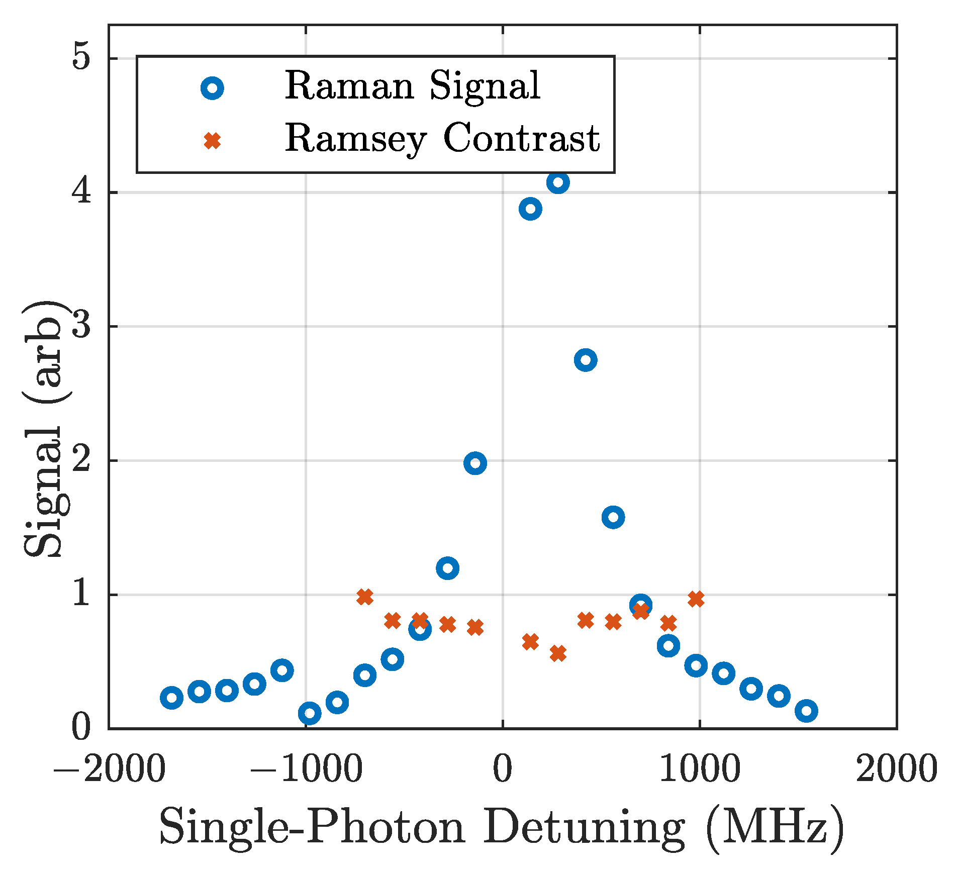
The demonstration of Ramsey interference in our system provided us with more opportunities to optimize and characterize the experiment. Figure 14 shows the strength of the Raman signal (blue dots and orange fit) and the coherence as measured by contrast in a Ramsey experiment (purple dots) as a function of single-photon detuning. Unlike the Raman signal that we expect to simply fall off with increasing detuning, as shown in the orange trace, the Ramsey signal is subject to competing factors.
In order to characterize the Raman and Ramsey signals, we define two quantities: the signal-above-background (SAB), which is defined exactly as it sounds, and we can define contrast (C) as
where is the first local minimum to the right of the central fringe. The SAB should increase with decreasing detuning (as with Raman spectra). Consider the case of a pulse that is less than a pulse; the closer you are to resonance, the closer you are to the -pulse condition (with a larger signal). Contrast should remain constant for all frequencies until one comes too close to resonance, at which point spontaneous emission cannot be ignored. Figure 14 shows the Raman spectra amplitude (in arbitrary units) and contrast overlaid on top of each other to illustrate the trade-off between signal and contrast (maximizing signal without appreciably sacrificing contrast). Of note is that there is a small range of frequencies for which we could not take data because the effects of spontaneous emission overwhelmed the detection apparatus.
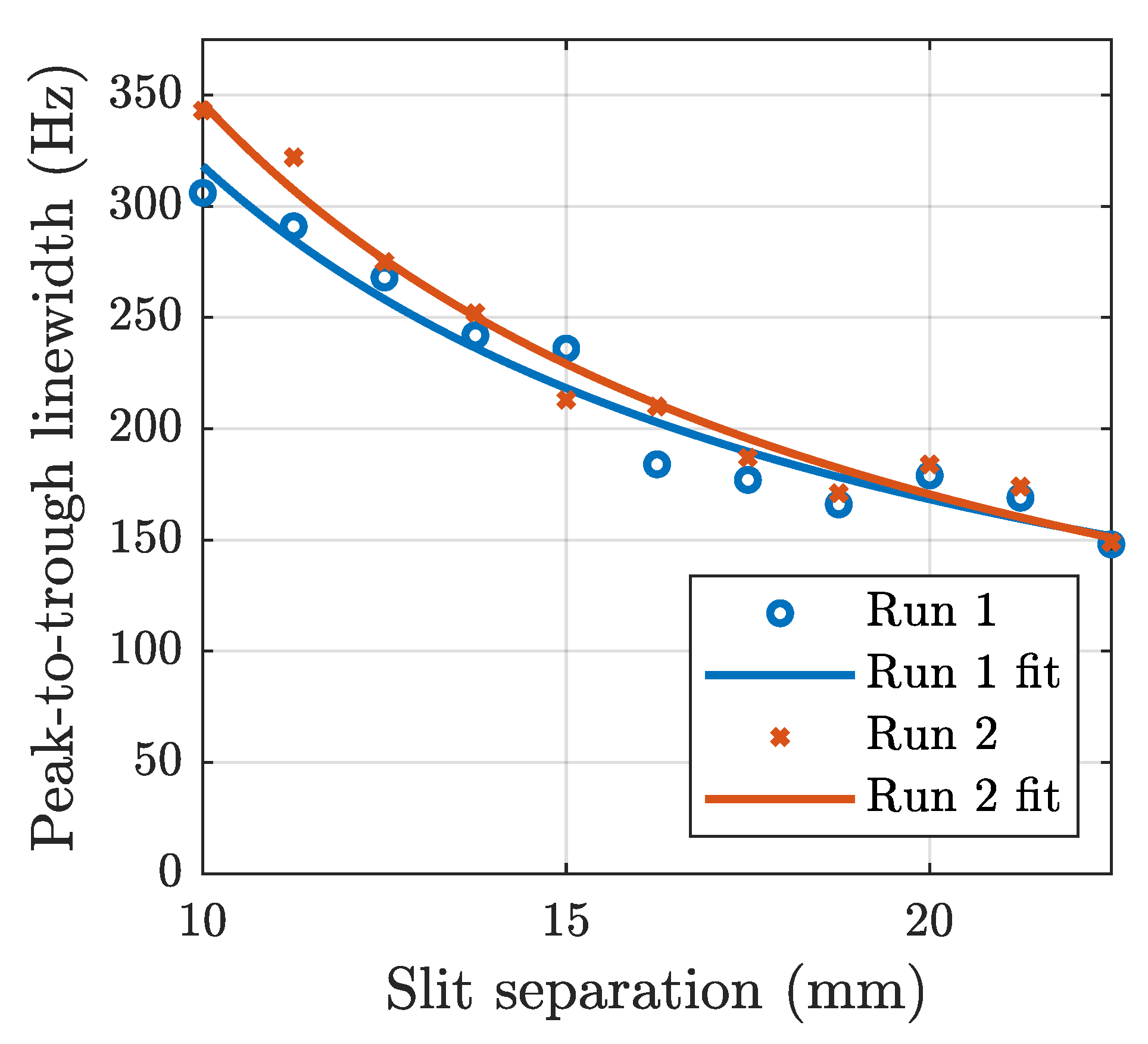
Figure 15 is a measurement of the fringe linewidth as a function of physical beam separation. Linewidth here is defined as the frequency difference between the center of the central fringe and the first trough to its right (higher frequency). Note that while the contrast did depend on the power balance between the two Raman beams making up the Ramsey interferometer, it remained constant with a constant power ratio between the two different frequency components. Furthermore, the trough location does not depend on power, so increasing the slit separation (with slits moving farther out in the Airy disk) does not affect the experiment. We expect it to vary inversely with beam separation [36]; all of our measurements are in qualitative agreement with this expectation.
7. Conclusions
In this paper, we have presented the details of our apparatus that was built to study interference in continuous beam atom interferometers with low average atom velocity. We characterized the atomic source, focusing on measurement of both the longitudinal and transverse velocities. The former was measured using a pulsed atomic source and the latter with imaging of the fluorescence from the atomic beam. We described our lock-in detection method to eliminate contamination of the desired signal by the strong background. We described our method for generation of the Raman fields and our methods for using them to optimize parameters in our setup such as power ratio to eliminate the AC Stark shift, magnetic field settings, single-photon detuning, and total power level. Finally, we presented some representative Raman and Ramsey spectra and optimized the operating parameters for Ramsey spectroscopy. Our results show that, despite the residual longitudinal velocity spread and the fairly high transverse velocity spread, a robust interference signal is observable. All the work described in this paper was performed in the Doppler-free configuration. Future work will involve either reflecting the Raman beam back itself or bringing in the Raman beams from opposite directions to be in the Doppler-sensitive configuration. This will be the starting point for future work.
Author Contributions
Conceptualization, F.A.N.; methodology, M.P.M., J.G.L. and F.A.N.; software, J.G.L.; validation, M.P.M., J.G.L. and F.A.N.; formal analysis, M.P.M., J.G.L. and F.A.N.; investigation, M.P.M., J.G.L. and F.A.N.; resources, F.A.N.; data curation, F.A.N.; writing—original draft preparation, M.P.M. and F.A.N.; writing—review and editing, M.P.M., J.G.L. and F.A.N.; visualization, M.P.M. and J.G.L.; supervision, F.A.N.; project administration, F.A.N.; funding acquisition, F.A.N. All authors have read and agreed to the published version of the manuscript.
Funding
This research was funded by the Office of the Secretary of Defense (OSD) grant number [N0017318WX00123] and the Integrated Warfare Systems (IWS) Office grant number [N0002420WX10409].
Acknowledgments
FAN wishes to thank George Welch for numerous fruitful discussions and assistance in the laboratory.
Conflicts of Interest
The authors declare no conflict of interest. The funders had no role in the design of the study; in the collection, analyses, or interpretation of data; in the writing of the manuscript, or in the decision to publish the results.
Appendix A
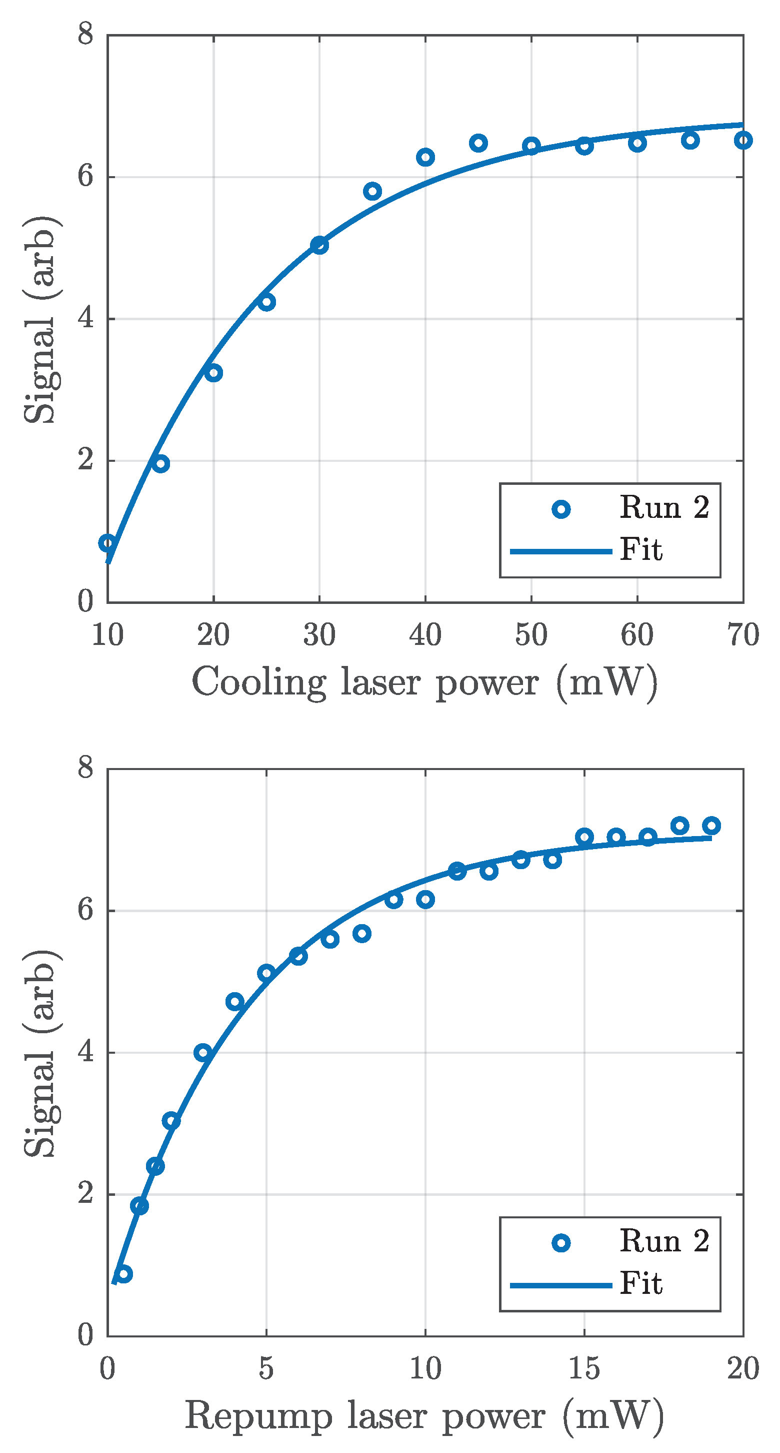
For these experiments, the detection laser was simply a circular beam of approximately 2 mm diameter that was sent into the chamber along a vertical direction through one of the top viewports. Due to the shape and size of the laser beam, only the atoms with small transverse velocity in the horizontal direction were detected, although atoms with larger transverse velocity in the vertical direction were detected. Subsequent experiments utilized a shaped detection beam (see Section 4.1). The detection laser power was held fixed at about 5 mW—a power level that roughly optimized the signal from the fluorescing atoms above the background caused by light scattering off the windows—and the frequency was scanned around the cooling transition at about 10 Hz. Light from the fluorescing atoms was collected with a collection lens and directed towards a photomultiplier tube, whose signal was amplified and filtered. The peak signal above background, which we used as a measure of atom flux, was recorded as a function of the total power from the cooling laser entering the MOT chamber.
Figure A1 (top) depicts the results of such a measurement. As is typical for atom traps, we see that the atom flux increased with increasing cooling beam power before saturating. Also displayed in the figure is a fit to a charging exponential function. Based on these data, we chose to operate the cooling laser at about 50 mW. At this level, the MOT was operating near the asymptotic limit, so that the system was fairly insensitive to power fluctuations of the cooling beam while not wasting power needlessly. A similar experiment was conducted to optimize the repump power and the results are depicted in Figure A1 (bottom). We chose to operate the repump laser at around 10 mW.
Figure A1.
(Top) Atomic beam fluorescence vs. cooling laser power along with a fit to an exponential function; these data were used to determine the optimal cooling laser power. (Bottom) Atomic beam fluorescence vs. repump laser power along with a fit to an exponential function; these data were used to determine the optimal repump laser power.

References
- Keith, D.W.; Ekstrom, C.R.; Turchette, Q.A.; Pritchard, D.E. An interferometer for atoms. Phys. Rev. Lett. 1991, 66, 2693–2696. [Google Scholar] [CrossRef]
- Carnal, O.; Mlynek, J. Young’s double-slit experiment with atoms: A simple atom interferometer. Phys. Rev. Lett. 1991, 66, 2689–2692. [Google Scholar] [CrossRef]
- Riehle, F.; Kisters, T.; Witte, A.; Helmcke, J.; Bordé, C.J. Optical Ramsey spectroscopy in a rotating frame: Sagnac effect in a matter-wave interferometer. Phys. Rev. Lett. 1991, 67, 177–180. [Google Scholar] [CrossRef]
- Kasevich, M.; Chu, S. Atomic interferometry using stimulated Raman transitions. Phys. Rev. Lett. 1991, 67, 181–184. [Google Scholar] [CrossRef]
- Kasevich, M.; Chu, S. Measurement of the gravitational acceleration of an atom with a light-pulse atom interferometer. Appl. Phys. B Photophys. Laser Chem. 1992, 54, 321–332. [Google Scholar] [CrossRef]
- Baudon, J.; Mathevet, R.; Robert, J. Atomic interferometry. J. Phys. B-At. Mol. Opt. Phys. 1999, 32, R173–R195. [Google Scholar] [CrossRef]
- Cronin, A.D.; Schmiedmayer, J.; Pritchard, D.E. Optics and interferometry with atoms and molecules. Rev. Mod. Phys. 2009, 81, 1051–1129. [Google Scholar] [CrossRef]
- Lepoutre, S.; Jelassi, H.; Trenec, G.; Buechner, M.; Vigue, J. Atom interferometry as a detector of rotation and gravitational waves: Comparison of various diffraction processes. Gen. Relativ. Gravit. 2011, 43, 2011–2025. [Google Scholar] [CrossRef] [Green Version]
- Barrett, B.; Geiger, R.; Dutta, I.; Meunier, M.; Canuel, B.; Gauguet, A.; Bouyer, P.; Landragin, A. The Sagnac effect: 20 years of development in matter-wave interferometry. C. R. Phys. 2014, 15, 875–883. [Google Scholar] [CrossRef] [Green Version]
- Geiger, R.; Landragin, A.; Merlet, S.; Pereira Dos Santos, F. High-accuracy inertial measurements with cold-atom sensors. AVS Quantum Sci. 2020, 2, 024702. [Google Scholar] [CrossRef]
- Barrett, B.; Bertoldi, A.; Bouyer, P. Inertial quantum sensors using light and matter. Phys. Scr. 2016, 91, 053006. [Google Scholar] [CrossRef]
- Bongs, K.; Holynski, M.; Vovrosh, J.; Bouyer, P.; Condon, G.; Rasel, E.; Schubert, C.; Schleich, W.P.; Roura, A. Taking atom interferometric quantum sensors from the laboratory to real-world applications. Nat. Rev. Phys. 2019, 1, 731–739. [Google Scholar] [CrossRef] [Green Version]
- Fang, B.; Dutta, I.; Gillot, P.; Savoie, D.; Lautier, J.; Cheng, B.; Garrido Alzar, C.L.; Geiger, R.; Merlet, S.; Pereira Dos Santos, F.; et al. Metrology with Atom Interferometry: Inertial Sensors from Laboratory to Field Applications. J. Phys. Conf. Ser. 2016, 723, 012049. [Google Scholar] [CrossRef] [Green Version]
- Narducci, F.A.; Black, A.T.; Burke, J.H. Advances toward fieldable atom interferometers. Adv. Phys. X 2022, 7, 1946426. [Google Scholar] [CrossRef]
- Gustavson, T.L.; Bouyer, P.; Kasevich, M.A. Precision Rotation Measurements with an Atom Interferometer Gyroscope. Phys. Rev. Lett. 1997, 78, 2046–2049. [Google Scholar] [CrossRef] [Green Version]
- Gustavson, T.; Landragin, A.; Kasevich, M. Rotation sensing with a dual atom-interferometer Sagnac gyroscope. Class. Quantum Gravity 2000, 17, 2385–2398. [Google Scholar] [CrossRef] [Green Version]
- McGuirk, J.M.; Foster, G.T.; Fixler, J.B.; Snadden, M.J.; Kasevich, M.A. Sensitive absolute-gravity gradiometry using atom interferometry. Phys. Rev. A 2002, 65, 033608. [Google Scholar] [CrossRef] [Green Version]
- Xue, H.; Feng, Y.; Chen, S.; Wang, X.; Yan, X.; Jiang, Z.; Zhou, Z. A continuous cold atomic beam interferometer. J. Appl. Phys. 2015, 117, 094901. [Google Scholar] [CrossRef] [Green Version]
- Xie, W.; Wang, Q.; He, X.; Fang, S.; Yuan, Z.; Qi, X.; Chen, X. A cold cesium beam source based on a two-dimensional magneto-optical trap. AIP Adv. 2022, 12, 075124. [Google Scholar] [CrossRef]
- Müller, T.; Gilowski, M.; Zaiser, M.; Berg, P.; Schubert, C.; Wendrich, T.; Ertmer, W.; Rasel, E.M. A compact dual atom interferometer gyroscope based on laser-cooled rubidium. Eur. Phys. J. D 2009, 53, 273–281. [Google Scholar] [CrossRef]
- Lu, Z.T.; Corwin, K.L.; Renn, M.J.; Anderson, M.H.; Cornell, E.A.; Wieman, C.E. Low-Velocity Intense Source of Atoms from a Magneto-optical Trap. Phys. Rev. Lett. 1996, 77, 3331–3334. [Google Scholar] [CrossRef] [PubMed]
- Schoser, J.; Batär, A.; Löw, R.; Schweikhard, V.; Grabowski, A.; Ovchinnikov, Y.B.; Pfau, T. Intense source of cold Rb atoms from a pure two-dimensional magneto-optical trap. Phys. Rev. A 2002, 66, 023410. [Google Scholar] [CrossRef]
- Kwolek, J.; Black, A. Continuous Sub-Doppler-Cooled Atomic Beam Interferometer for Inertial Sensing. Phys. Rev. Appl. 2022, 17, 024061. [Google Scholar] [CrossRef]
- Meng, Z.X.; Yan, P.Q.; Wang, S.Z.; Li, X.J.; Feng, Y.Y. Closed-Loop Dual-Atom-Interferometer Inertial Sensor with Continuous Cold Atomic Beams. arXiv 2022. [Google Scholar] [CrossRef]
- Riis, E.; Weiss, D.S.; Moler, K.A.; Chu, S. Atom funnel for the production of a slow, high-density atomic beam. Phys. Rev. Lett. 1990, 64, 1658–1661. [Google Scholar] [CrossRef]
- Kellogg, J.R.; Schlippert, D.; Kohel, J.M.; Thompson, R.J.; Aveline, D.C.; Yu, N. A compact high-efficiency cold atom beam source. Appl. Phys. B 2012, 109, 61–64. [Google Scholar] [CrossRef] [Green Version]
- Manicchia, M.P.; Lee, J.; Welch, G.R.; Mimih, J.; Narducci, F.A. Construction and characterization of a continuous atom beam interferometer. J. Mod. Opt. 2020, 67, 69–79. [Google Scholar] [CrossRef]
- Manicchia, M. Construction and Characterization of a Dual Atomic Beam Accelerometer/Gyroscope. Ph.D. Thesis, Naval Postgraduate School, Monterey, CA, USA, 2020. [Google Scholar]
- Steck, D. Rubidium 85 D Line Data. Revision 2.2.3. Available online: http://steck.us/alkalidata (accessed on 9 July 2021).
- Inc., Wolfram Research. Clebsch-Gordan Calculator-Wolfram|Alpha; Inc., Wolfram Research: Champaign, IL, USA, 2021. [Google Scholar]
- Kimble, H.J.; Dagenais, M.; Mandel, L. Photon Antibunching in Resonance Fluorescence. Phys. Rev. Lett. 1977, 39, 691–695. [Google Scholar] [CrossRef] [Green Version]
- Dagenais, M.; Mandel, L. Investigation of two-time correlations in photon emissions from a single atom. Phys. Rev. A 1978, 18, 2217–2228. [Google Scholar] [CrossRef]
- Narducci, F.A. Photon Correlation Effects in Single and Multi-Atom Systems. Ph.D. Thesis, University of Rochester, Department of Physics and Astronomy,, Rochester, NY, USA, 1996. [Google Scholar]
- DeSavage, S.; Gordon, K.; Clifton, E.; Davis, J.; Narducci, F. Raman resonances in arbitrary magnetic fields. J. Mod. Opt. 2011, 58, 2028–2035. [Google Scholar] [CrossRef]
- DeSavage, S.; Davis, J.; Narducci, F. Controlling Raman resonances with magnetic fields. J. Mod. Opt. 2013, 60, 95–102. [Google Scholar] [CrossRef]
- Meldrum, A.; Manicchia, M.; Davis, J.P.; Narducci, F.A. Raman spectroscopy using a continuous beam from a 2D MOT. In Proceedings of the Steep Dispersion Engineering and Opto-Atomic Precision Metrology XI, San Francisco, CA, USA, 2 February 2018; SPIE: Bellingham, CA, USA, 2018; Volume 10548, pp. 114–124. [Google Scholar] [CrossRef]
- Ramsey, N.F. A Molecular Beam Resonance Method with Separated Oscillating Fields. Phys. Rev. 1950, 78, 695–699. [Google Scholar] [CrossRef]
- Ramsey, N.F. Molecular Beams; Oxford University Press: Oxford, UK; New York, NY, USA, 1990. [Google Scholar]
Figure 1.
A schematic representation of our experimental setup. In the left (yellow) 2D-MOT section, a rubidium getter is used as an atomic source. Standard 2D-MOT cooling and repump beams with the correct circular polarization states are directed into the chamber and retroreflected through a quarter-waveplate. Another similar cooling beam (not depicted) travels vertically, into and out of the page. Prior to the 2D-MOT beam entering the interferometry section to the right (green) through a small aperture, an optical pumping beam is applied to optically pump the atoms to the dark state (or to shutter the atomic beam). The result is a diverging beam of cooled atoms traveling along the central axis of the science chamber, through the interferometry region from left to right. In this interferometry section, we have three areas of optical access where we apply the interferometry beams and implement our detection setup.

Figure 2.
Frequency difference between fluorescence from atoms in the atomic beam and a simultaneous saturated absorption spectrum. The difference suggested a most probable atomic beam velocity of ∼4.4 m/s.
Figure 2.
Frequency difference between fluorescence from atoms in the atomic beam and a simultaneous saturated absorption spectrum. The difference suggested a most probable atomic beam velocity of ∼4.4 m/s.

Figure 3.
Time-of-flight detection signal of optically pumped atoms. The amplitude peak corresponds to the most probable speed of 6.4 m/s.
Figure 3.
Time-of-flight detection signal of optically pumped atoms. The amplitude peak corresponds to the most probable speed of 6.4 m/s.

Figure 4.
Measurement of the atomic beam fluorescence versus auxiliary laser frequency with no optical pumping (solid purple trace), optical pumping on the transition (dashed yellow trace), and optical pumping on the transition (dotted and dashed orange trace). The single-pass absorption signal from the scanning auxiliary laser (dotted blue trace) is included as a frequency reference (and here one can see the 1.5 GHz frequency shift due to our selection of the red-shifted Raman beam as the auxiliary laser). Of note, not only is more difficult to produce with our equipment than , but it also provides less efficient optical pumping.

Figure 5.
The optical setup used to create the light for optical pumping and atom beam switching. Input light, at frequency , from the cooling laser (red) passed through an AOM being driven at , producing 0-order (blue) and -order (green) output beams. These were retroreflected in a double-pass cat’s eye setup, without the usual iris blocking the 0-order beam. The result was that the output mode we wished to use (magenta) contained two frequency components—one from light that was shifted down in frequency on both passes (at frequency ), and the other from light that was not shifted during either pass (at frequency ). The unwanted second-pass output also contained two frequencies that were not of use to our experiment (at frequency and ), which we blocked with an iris. A waveplate in the retroreflection arm, along with a polarizing beamplitting cube on the input side of the AOM, was used to spatially separate the input beam from the output beam of interest.

Figure 6.
Detected fluorescence with cooling lasers for the 2D-MOT on (blue trace) and off (red trace).
Figure 6.
Detected fluorescence with cooling lasers for the 2D-MOT on (blue trace) and off (red trace).

Figure 7.
Raw Raman spectrum (blue) and output from the lock-in amplifier (red).

Figure 8.
(Top) Depiction of the optics scheme used to create the two frequency-shifted Raman beams from a single laser. When the light from the Raman laser passes through the AOM, the 1st-order beam (red dotted arrow) is red-shifted by 1517.866 MHz. After retroreflection of the unshifted 0th-order beam, the 1st-order beam from the second pass (blue dashed arrow) is blue-shifted by 1517.866 MHz. These two beams are then combined via a 2-to-1 PM fiber and taken to the experiment (dashed and dotted beam at bottom of the diagram). (Bottom) Photo of the optics scheme used to create the two frequency-shifted Raman beams from a single laser.

Figure 9.
Depiction of the optics used to create the separate physical Raman beams from the single Raman laser. The beam size is manipulated so that a mask may be used to make the beams; as an example, this depiction shows a three-beam mask used for spin-echo interference. The polarization produced depends upon whether the configuration is Doppler-sensitive or not (this depiction shows same-handed circular polarization for a Doppler-free, co-propagating scheme).

Figure 10.
Experimentally measured clock transition frequency as a function of applied magnetic field longitudinal to the Raman beam propagation direction.
Figure 10.
Experimentally measured clock transition frequency as a function of applied magnetic field longitudinal to the Raman beam propagation direction.

Figure 11.
A typical measurement of Rabi oscillations as a function of laser intensity. The x-axis is scaled to the maximum power attainable and the y-axis is scaled to the maximum fluorescent intensity.
Figure 11.
A typical measurement of Rabi oscillations as a function of laser intensity. The x-axis is scaled to the maximum power attainable and the y-axis is scaled to the maximum fluorescent intensity.

Figure 12.
Experimentally measured clock transition in the Doppler-free configuration. The peak is not centered about 0 detuning because of the presence of a small second-order Zeeman shift.
Figure 12.
Experimentally measured clock transition in the Doppler-free configuration. The peak is not centered about 0 detuning because of the presence of a small second-order Zeeman shift.

Figure 13.
Experimentally measured Doppler-free Ramsey interference pattern.

Figure 14.
Experimentally measured Raman signal above background data points (blue circles) and Ramsey contrast (red crosses) as a function of detuning.
Figure 14.
Experimentally measured Raman signal above background data points (blue circles) and Ramsey contrast (red crosses) as a function of detuning.

Figure 15.
Experimentally measured Ramsey fringe linewidth (frequency difference between the central peak and the adjacent trough) as a function of physical beam spacing for two typical runs. The data points are fit to , where A = 2995 Hz * mm, d is the slit spacing, and c = 18.6 Hz for run 1, with A = 3516 Hz * mm and c = −5.30 Hz for run 2.

Disclaimer/Publisher’s Note: The statements, opinions and data contained in all publications are solely those of the individual author(s) and contributor(s) and not of MDPI and/or the editor(s). MDPI and/or the editor(s) disclaim responsibility for any injury to people or property resulting from any ideas, methods, instructions or products referred to in the content. |
© 2023 by the authors. Licensee MDPI, Basel, Switzerland. This article is an open access article distributed under the terms and conditions of the Creative Commons Attribution (CC BY) license (https://creativecommons.org/licenses/by/4.0/).
Share and Cite
MDPI and ACS Style
Manicchia, M.P.; Lee, J.G.; Narducci, F.A. Characterization of a Continuous Beam Cold Atom Ramsey Interferometer. Atoms 2023, 11, 51. https://doi.org/10.3390/atoms11030051
AMA Style
Manicchia MP, Lee JG, Narducci FA. Characterization of a Continuous Beam Cold Atom Ramsey Interferometer. Atoms. 2023; 11(3):51. https://doi.org/10.3390/atoms11030051
Chicago/Turabian StyleManicchia, Michael P., Jeffrey G. Lee, and Frank A. Narducci. 2023. "Characterization of a Continuous Beam Cold Atom Ramsey Interferometer" Atoms 11, no. 3: 51. https://doi.org/10.3390/atoms11030051
Note that from the first issue of 2016, this journal uses article numbers instead of page numbers. See further details here.