
EUV Beam–Foil Spectra of Germanium and a Blind-Spot Problem in Spectroscopy


Ruhr-Universität Bochum, Fakultät für Physik und Astronomie, AIRUB, 44780 Bochum, Germany
Atoms 2023, 11(3), 45; https://doi.org/10.3390/atoms11030045
Submission received: 2 February 2023
/
Revised: 26 February 2023
/
Accepted: 28 February 2023
/
Published: 2 March 2023
(This article belongs to the Special Issue Editorial Board Members’ Collection Series: Atomic Collision and Atomic Spectroscopy)
Abstract
:Beam–foil extreme-ultraviolet survey spectra of Ge () are presented. The data have been garnered at the performance limit of the heavy-ion accelerator available, with a correspondingly limited statistical and calibrational reliability. However, the Ge spectra have been recorded at various delays after excitation, and this technique points to a possible blind spot in some other spectroscopic techniques, and thus in the literature coverage. A similarly patchy coverage can be noted in various atomic structure computations. The experimental and theoretical gaps seem to be correlated.
1. Introduction
One of the most comprehensive compilations of extreme ultraviolet (EUV) wavelength data of multiply charged ions of many elements is the online database ASD maintained and curated by the US National Institute of Standards and Technology (NIST) [1,2].
Other examples are the combination of experimental data and computations by Fawcett [3], the compilation by Kelly [4], and the CHIANTI project [5,6,7]. CHIANTI addresses mostly solar EUV spectra and therefore is largely limited to elements of high solar abundance, that is, to mostly even-Z elements up to Ni (). The other databases mentioned have no such special interest background, but they still reflect the historic funding situation, which, for example, for a while targeted elements up to Ni (“including the iron group”). Spectral data on heavier elements consequently are much scarcer.
After a first wave of fusion-motivated spectral studies and data compilations in the 1970s, a second wave (in the second half of the 1980s) included Mo () as a heat-resilient element and component of stainless steel vacuum vessels. Consequently, a number of measurements at tokamaks and laser-produced plasmas was funded that addressed elements up to Mo, for example those by Kaufman, Rowan and Sugar [8,9,10,11,12] of the National Bureau of Standards (NBS), the precursor of the aforementioned NIST, and experiments undertaken at various laser-produced plasma sources, including, for example, those by Litzén, Ekberg and Jupén from Lund university [13,14,15,16]. The data look rich, and the analyses comprehensive, but incidentally there appears to be a blind spot that possibly relates to, both, the light sources used and the computational resources employed for atomic structure calculations. This gap in the coverage has shown first in the attempt to analyse so-called delayed beam–foil spectra of Si-like ions of iron group elements. The lowest level in the second-but-lowest configuration, 3s3p, is a S level, but neither the level nor the expected two intercombination decay branches to 3s3p P were to be found in the spectral tables available at the time, neither from observation nor from computation. Incidentally, the corresponding spectral lines in the first few members of the isoelectronic sequence were already known, and they had been essential in recognising that Jupiter’s moon Io has volcanoes that spew sulfur and thus feed a plasma torus along its orbit [17]. Were the lines not seen in heavier elements, because the pointer by computational prediction was insufficiently accurate, or were the lines and levels largely disregarded by theory, because the reported spectra did not show them. According to the Ritz principle, in a variational calculation the lowest level of a given parity can be determined with the highest accuracy, but the 3s3p S level was not even mentioned in several studies.
Theory eventually explained the particular computational difficulties encountered with this level [18]. In the Si-like ions, the challenge lies in the mixing of not just of two near-by levels of different multiplicity (as is usually the case in two-electron ions), but of three (3s3pS, P and D), as well as in pronounced cancellation effects in the decay of one of the mixing partners. A similar level, 2s2pS, is found in C-like ions (see [19] and references therein). For lack of time resolution, the absolute decay rate of the quintet level is usually not measured. However, the branch fractions show a significant variation along the isoelectronic sequence, which reflects the complex level mixing in such an atomic system—and this effect can be observed without time resolution. Not long after, beam–foil spectroscopic measurements succeeded in demonstrating the line patterns of such intercombination transition arrays [20] and identified some of the lines of interest in spectra of the solar corona [21,22,23,24]. The beam–foil work yielded level lifetimes and thus transition rates in several elements. The analysis revealed a considerable scatter of the predictions for the iron group elements, in particular for the low-Z members of the isoelectronic sequence [25]. At low Z, the level lifetimes are too long for measurements using beam–foil techniques. In that range, an atomic lifetime measurement on P, using an ion trap [26], and the result of one computation [27] eventually agreed with each other.
The question arises why some groups of data may have eluded observation as well as theoretical treatment. Since 3s–3p transitions have been discussed in the above papers, the emphasis of the present discussion is on 3p–3d transitions in ions with a more than half-filled 3p shell in the ground state, that is, on P- through Ar-like ions. I am using the occasion of “Six decades of beam-foil spectroscopy” [28,29,30,31,32,33,34] to discuss this experimental technique more generally, recalling its strong points as well as its problems and limitations. The present report describes EUV spectra obtained by the beam–foil technique on ions of Ge. For various reasons (largely discussed in [35,36,37]) the new spectra do not (yet) add to the available line identifications in the literature. Nevertheless the data are clear enough to support the hypothesis of a ‘blind spot’ that some spectroscopic techniques and theoretical treatments may have suffered from. This is illustrated by means of the unique properties of time-resolved EUV spectroscopy using the beam–foil technique.
2. Experiment
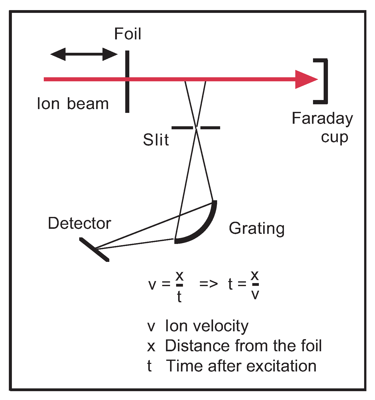
A schematic of the measurement arrangement is shown in Figure 1. A practically mono-energetic and mono-isotopic fast ion beam from a heavy-ion accelerator is directed through a thin (usually) carbon foil in which the ions acquire a new charge state distribution, lose a small fraction of their energy, but continue on a trajectory and with a velocity not much different from before (a case well approximated by ions colliding with an electron gas; collisions with the more massive atomic cores are much less numerous). Excitation of the ions happens inside the dense foil material within a travel time of a few femtoseconds; a spatial observation zone of the ion beam at a distance from the foil corresponds to a detection at a time after excitation as well as in a time interval that can be chosen on the scale from dozens of picoseconds to many nanoseconds.
Beam–foil spectroscopy offers time-resolved observations that can be used to obtain prompt and delayed spectra or decay curves of individual levels. In various ways, the beam–foil light source can be considered a didactical tool. A single element (isotope) contributes, a range of charge states can be predetermined, observations feature inherent time resolution so that decay curves of given spectral features (at a known wavelength setting) or spectra at a given time after excitation can be recorded, with the production at high electron density (in the foil) separated spatially from the observation in high vacuum. Drawbacks are Doppler shifts and the associated problem of an accurate wavelength calibration.
The spectra shown in this study have been obtained at the Bochum Dynamitron tandem accelerator laboratory (DTL), where a 4 MV tandem accelerator equipped with a sputter ion source [38,39] was available. In such a tandem accelerator, negative ions enter at ground potential and are accelerated toward a high voltage terminal. With a terminal voltage U at about 4 MV, singly charged ions attain a kinetic energy of E 4 MeV. In the terminal, the ions pass through a dilute gas target and lose typically several electrons; the maximum of the charge state distribution lies between charge states and . The positively charged ions are accelerated further by using the same voltage drop again, but now from positive high potential to ground. For these two charge state fractions, the total kinetic energy (E then reaches either 16 or 20 MeV. The desired combination of ion beam energy and charge state is selected by separating the various ion beam fractions in a magnetic field; only the selected ion beam is guided to the experiment, where it is sent through a thin carbon foil of areal density 10 μg/cm2. A grazing-incidence spectrometer (McPherson Model 247) equipped with an m grating of groove density 600 ℓ/mm disperses the EUV radiation emitted by the excited ions. A channeltron serves as the detector behind the exit slit of the scanning instrument.
At the ion beam energy of 20 MeV in the above example, the charge state distribution after passage through the exciter foil has a maximum near (the charge state distributions refer to the investigations by Shima et al. [40]). This would correspond to the K-like spectrum of Ge, Ge XIV. However, while this spectrum (in the EUV) has not yet been studied by beam–foil spectroscopy, the extension of the Bochum group’s preceding work on ions of the iron group elements (see [36,37]) called for higher charge states which required higher ion beam energies, which in turn required higher charge states than from the gas stripper in the accelerator high voltage terminal. Actually, the highest charge state for which an ion beam fraction was large enough to yield a practically useful detector signal (after charge-state modification and excitation of the fast ions in the passage through the foil) behind the exit slit of the spectrometer was , with an ion beam energy of 36 MeV. At this energy, the Shima tables [40] indicate a maximum charge state after ion–foil interaction of (Cl-like), with charge state fractions that might suffice for an observable signal for (Si-like) to (Ca-like). (The earlier measurements on Zn () (see [36]) had been limited to ion beam energies of 22 MeV and 28 MeV, respectively, because the ion source output for Zn had been so much lower that the charge state fraction from the accelerator had been the highest one useable.) For 36 MeV Ge ions the beam current (particle current) amounted to about 0.03 μA, which was barely sufficient for recording meaningful data.
3. Data
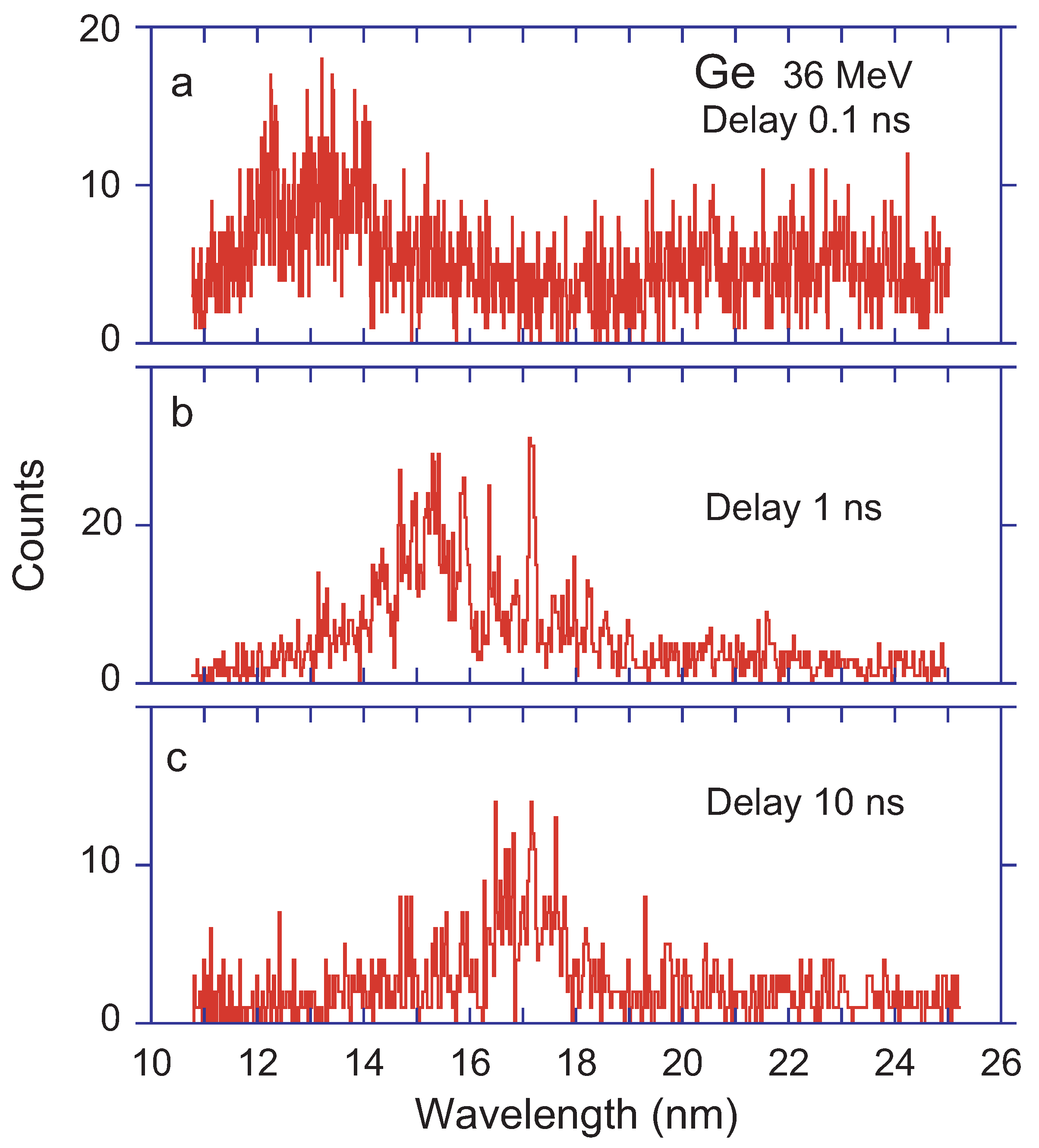
The Ge ion beam at Bochum had a velocity of about 1 cm/ns (roughly 3% of the speed of light). Measurements were taken close to the foil (but positioning the foil just outside the field-of-view of the spectrometer, in order to suppress the quasi-continuum of emission by the multitude of core-excited ions), at 1 cm and at 10 cm downstream of the foil, that is, of almost prompt emission and after delays of 1 ns and 10 ns. Each of the spectra (see Figure 2) shows a fair number of line-like spectral structures the positions of which reflect energy level differences in the atomic emitters, and these, of course, do not vary with time. However, the line intensities depend on the level lifetimes, and those line intensities seem to fall in groups that result in clumps of a common behaviour. For different delays after excitation, the line clumps appear at different wavelengths.
For the ions encountered here, the dominant transitions are expected to be 3p–3d transitions at the shorter (up to = 19 nm) and 3s–3p transitions at the longer wavelengths (beyond = 19 nm, that is, mostly outside of the present data range), giving rise (among others) to resonance and intercombination lines. The spectrometer field-of-view covers more than a decay length (level lifetime × ion velocity) for resonance transitions, but only a fraction of a decay length for typical intercombination decays. Thus, the signal is accordingly weaker for the latter (by an order of magnitude or more), even if the initial upper-level population may have been equal. Further corrections arise from the spectrometer slit width and for the signal normalisation to the ion beam charge collected on the Faraday cup. For example, the signal ratio of the line profile at wavelength 17.2 nm (Figure 2b,c) suggests a decrease of the signal by about a factor of about three, corresponding to an upper-level lifetime on the order of 10 ns. Consequently, this line is not expected to contribute much more to Figure 2a than to Figure 2b. However, the spectrum in Figure 2a was recorded with a much shorter accumulation time per channel and much narrower slits. Thus, an amplitude of about two counts per channel may be assumed for this line in the prompt spectrum, which would fit to a blend with a multitude of equally weak other decays in the spectrum of Figure 2a.
Spectrum analysis is interested in the identities of (all) the individual lines, with accurate wavelengths and, if possible, decay curves and relative line intensities from observations at different ion beam energies so that (possibly) via atomic structure calculations and spectrum modelling the spectrum number and transition can be determined. The given accelerator power was barely sufficient to produce the ion beam for the spectra in Figure 2. The option to pursue further experiments with systematic variations was not available, nor the resources available for establishing an accurate wavelength calibration by carefully orchestrated reference measurements with several other elements. The rough estimate of a 0.5% wavelength accuracy is not much better than most of the theoretical attempts discussed below. However, the graphical presentation of the survey spectra in Figure 2 is good enough for orientation. A wavelength table with only moderately accurate wavelengths might even be misleading until a proper reference wavelength can be established, and for this reason none is given here. The general properties of the Ge spectra in Figure 2 are similar to the corresponding spectra of Ti and heavier iron group elements recorded since the 1980s at the Bochum accelerator laboratory. Most physics projects using this apparatus aimed at details in very limited wavelength ranges, and the general interpretation of the overall spectrum needed to mature. In this sense, the presentation and discussion of the three Ge spectra in Figure 2 actually is a “first”.
Soon after the presently reported Ge measurements had been performed, the experimental apparatus had to be dismantled for good (that is, for other priorities in the institution). Why then report on such an evidently incomplete study of limited precision at all? There is some “meta-information" in the data that to me is of sufficient interest to discuss, and that aspect is what makes this report a ‘Viewpoint’ instead of an ‘Article’ that would have to concentrate on hard data. This “meta-information" emerges from the discussion below, from the spectral bumps in the time-resolved spectra above, and from the ranges of literature data and of most earlier atomic structure computations.
4. Literature Data and Atomic Structure Computations
With the aim of eventually identifying the lines in the spectra of Figure 2, it seems obvious that one should find out what is known already, and if not outright known, what is available from predictive atomic structure computations. Of course, computing resources have become much more achievable than they were in “the early days” (half a century ago), and more complete and more accurate computations can be performed today. There is a time component in what has emerged as my ’blind spot’ hypothesis, in several senses, and the reader is asked to suffer a bit of historic development description on the way to the present situation.
4.1. Literature Data
A search of the NIST ASD online database [2] for spectral lines of Ge ions of the expected charge states in the wavelength ranges of interest for interpreting the data in Figure 2 came up empty. This was surprising to me, since there are numerous reports on experimental EUV spectra that include Ge [8,9,10,11,12,13,14,15,16]. Maybe the wavelengths reported by NIST colleagues did not make the cut in the compilation process for the NIST database? Maybe the experiments happened not to cover the wavelength interval of this beam–foil work interest? Why were there some publications on term values, but no listings of the corresponding EUV wavelengths? Another compilation, by Raymond Kelly [4], had collected wavelength data irrespective of source which had been filtered by the merit of the original authors’ accuracy estimates (see Table 1). It shows that more than 30 years ago there were known Ge ion transitions in the wavelength range of present interest, often in charge states higher than reached in this experiment, and some of lesser accuracy. Actually, all of the respective data on Ge ions in medium-high charge states in [4] had been added in the decade (roughly the 1980s) since the publication of the original Kelly & Palumbo tables [41]. Considering only the charge states that are likely contributing to the present Ge spectra, it looks as if most of the (rather few) known lines coincide with the shorter-wavelength bump in Figure 2a, and none with the bump in Figure 2c. There are so many lines in the beam–foil spectra, and so few reported from the laser-produced plasma studies in the same spectral range that have used instruments with a roughly similar resolving power! At least it emerges that experimenters at other light sources have looked at the same wavelength range, but they did not see/classify many lines. The problem must lie somewhere else.
4.2. The Bumps in the Time-Resolved Ge Spectrum
The unique feature of the beam–foil data in Figure 2 is their time resolution. The structure of the bumps in the spectra changes with the time after excitation. The bump at 12–14 nm in the (almost) prompt spectrum (Figure 2a) corresponds to the wavelength range of 3p–3d resonance transitions in P- to K-like Ge ions [4]; the observation time window covers most of the short-lived level decays (level lifetimes < 0.1 ns). The bump in Figure 2b (at 14–19 nm) features a group of lines near 15 nm that is brightest under these conditions and likely originates from decays with an upper level lifetime on the order of 1 ns. A prominent line near 17.2 nm persists to the spectrum recorded at a delay of 10 ns (Figure 2c) and thus likely represents a level with a lifetime on that order of magnitude, with further lines of an even longer upper-level lifetime nearby. Apparently the three spectra represent three samples of decays with different upper-level lifetimes, which implies differences in the decay process and thus groups of levels with common peculiarities in the underlying atomic structure.
If the decays of the lines in the three bumps were of the same type, they might show a different lifetime range because of the variation in transition energy. However, that difference is on the order of 20%, and for the typical = 0 intra-shell transitions the lifetime difference would be of the same order, whereas the apparent lifetime spread in the data amounts to about two orders of magnitude, as is typical for transitions with spin change vs. transitions without. Moreover, since about a century Hund’s rule tells us that in a given electron configuration the term with the highest multiplicity lies lowest, a phenomenon recognised to result from the exchange interaction that, for example, in the He atom raises singlet levels above the correspondingly lowered triplet levels. It therefore seems likely that the shorter-wavelength lines in the Ge sample spectrum are from resonance transitions (with spin conservation), and the longer-wavelength and long-lifetime lines are from spin-changing (intercombination) transitions. Indeed, the lines listed in Table 1 that are quoted from the Kelly tables [4] are almost all from transitions without spin-change. A few spectral lines predicted by theory (see discussion below) suggest that certain intercombination transitions fall into the wavelength range of the longer-wavelength bump. Apparently the statistically mediocre beam–foil data of the present sample, because of their inherent time resolution, are nevertheless sufficient to point out that earlier measurements and theory have neglected a class of transitions that is essential for establishing the relative positions of the various term systems.
This effect has been seen before in beam–foil spectroscopy (especially clearly at the very same experimental set-up with its high ion beam current accelerator, see [20,21,22,23]). The fact that beam–foil spectroscopy sees a specific set of transitions differently from the observations at, for example, a laser-produced plasma is worth a more systematic discussion. Another point worth discussing is why certain intercombination decays have not been reported from various atomic structure computations.
5. Intercombination Transitions in Experiment and Theory
In the 19th century, the spectrum of (neutral) He seemed to indicate two separate term systems (of singlet and triplet levels, respectively), ascribed to orthohelium and parhelium, without an apparent crosslink. This interpretation led to the concept of Russell-Saunders or -coupling. Half a century ago, some German textbooks on atomic physics still presented He as a model case of spin conservation and barely hinted at the violations of the pure case. At the same time, intercombination transitions (with a spin change) had long been observed and correctly classified, and the He atom structure had been explained in detail by quantum mechanics since the 1920s. Apparently, basic knowledge and its textbook representation had become disconnected. With increasingly hot plasmas in fusion-test experiments, higher charge states were studied in which the steep iso-electronic increase of the transition rates of spin-changing transitions and of -forbidden transitions helped to render such lines visible and even useful for plasma diagnostics [42,43].
When our beam–foil group in the 1970s and early 1980s began to record spectra of Si, P and S (other groups did that at the same time, as we found out later), the literature information on intercombination transitions was still sparse, although in our spectra the intercombination line 3sS–3s3p P of Mg-like ions appeared brightly. For example, in the Kelly & Palumbo tables of 1978 [41] a wavelength of this line in Fe XV was obtained by Kelly’s own calculations. By 1984 an accurate wavelength value had been established by experiment (see [43]). At about the same time, Curtis & Ramanujam presented isoelectronic wavelength predictions for intercombination and -forbidden transitions in Mg-like ions [44], which largely relied on scaling relations to interpolate the few known values.
When there is little information in the wavelength tables, and only a few results are available from calculations of unproven predictive power, an experimenter is challenged in where to search, or how to label the many lines in a spectrum. Similarly, a theorist with limited computing power cannot be expected to meaningfully predict everything, and sensible approaches might choose the strongest signal lines (usually resonance lines of single- or few-electron ions) or a limited number of levels that the given computer can handle. For example, early attempts on atomic structure computations used few configurations or an averaging electron core plus a few orbitals of valence electrons (as in the Hartree-Fock with statistical exchange program package), or addressed only levels that connect to the ground term by transitions. The latter option (see [45]) included spin change, but excluded a few levels of very high spin. One may not miss the left-out levels, until for unforeseen reasons they suddenly become possibly interesting (see examples in [46]), nor in the next literature source checked—because many projects have the same limits on resources.
Data analysis nowadays is almost routinely aided by atomic structure computations following various approaches, as has been discussed recently by Jönsson et al. [47]. The computations yield results of various levels of accuracy. Some computations that are of limited accuracy can be adjusted to experimental data and then serve for reliable interpolations [48]. The reliability of atomic structure computations is highest (on the order of 10) for systems with a single electron in the valence shell and usually progressively poorer with more electrons in an open shell (say, 1% for inter-shell ground state transitions). Transitions between excited levels are predicted (and rarely stated) with accordingly larger uncertainties. This situation has been discussed in more detail and with numerous references elsewhere (for example, in [35,36,37]). Here I am pointing out just a few examples in Al- through Ar-like ions of Ge and nearby elements.
5.1. Quartet Levels in Al-like Ions
The 1993 table of Ge ion levels compiled by Sugar and Musgrove did not list the Ge XX 3s3p quartet levels nor all of the 3s3p3d quartet levels (for example, none of the 3s3p3d F levels) [49]. If atomic structure theory had been advanced enough to yield reliable predictions, the intercombination line multiplet Fe XIV 3s3p P–3s3p P should have been identified by that time in the solar corona EUV spectra analysed by Behring et al. and by Sandlin et al. [50,51], the latter of whom list tentative assignments of the structurally related Fe XXIII 2s2p P–2s2p P transitions. As soon as beam–foil spectroscopy identified a number of lines by their relative prominence in delayed spectra with the Fe XIV 3s3p P–3s3p P intercombination transitions, it became straightforward to combine the theoretical estimates with the not very precise wavelengths from beam–foil work and with accurately determined wavelengths of unidentified lines in the EUV spectrum of the solar corona and to thus establish the positions of the 3s3p P key levels of the quartet term system in Fe XIV as well as in other spectra of iron group elements [22].
Later beam–foil work and lifetime measurements on Al-like ions at a heavy-ion storage ring tracked other long-lived levels such as 3s3p3d F[52,53,54]. Again, the high-J levels had been left out from various theoretical predictions. Dedicated work shows how much more can be learned from a more complete computation [55]. That computation reaches up to (Ge), the element of the data in Figure 2. Incidentally, the theoretical work yields a term difference of two quartet levels that corresponds to a wavelength of 17.207 nm close to prominent lines that appear in the delayed spectra (Figure 2c). However, the terms involved in this prediction differ by 2 units of angular momentum, which suggests a low transition rate of the line even if the upper level was excited. Anyway, at the given ion beam energy, the spectrum Ge XX is not expected to contribute significantly.
5.2. Quintet Level Intercombination Decays in Si-like Ions
Si-like ions feature a 3s3p ground configuration with triplet and singlet levels (connected by -forbidden transitions) and consequently many singlet and triplet transitions that connect the ground configuration with higher configurations (3s3p, 3s3p3d, etc.) in which the multiplicity does not change. Apparently it was largely overlooked that the lowest excited odd-parity level belongs to the quintet term system. The 1993 table of Ge ion levels compiled by Sugar and Musgrove did not list any Ge XIX quintet level (nor the 3s3p3d F levels) [49]. The story of finding the 3s3pS level and its intercombination decays is similar to that of the above example for the Al-like ions [20,22]. The lines were detected in delayed beam–foil spectra that thus helped to identify much more accurately measured structures in solar corona spectra, while some otherwise remarkably accurate theoretical studies (such as [56]) did not even mention them. Table 2 lists the quintet decays (which lie outside of the range of the present beam–foil spectra) in order to show the variation and progress of wavelength prediction from early attempts [57] via interpolations of experimental data [15] to present-day results [58]. The (typical) offset between computed results [56] and measured data made it possible to deduce a corrected prediction for the rather long-lived Fe XIII 3s3p3d F level and to thus identify its decay in delayed beam–foil spectra as well as in solar corona spectra [23].
The computational treatment of Si-like ions has taken significant steps forward since then (see [58,62,63,64], some of which include results for Ge), while the interplay of experiment and computation goes on. Not quite settled, for example, is the position of the Fe XIII 3s3p3d F level which by an decay feeds the J = 3 level of the same term and thereby a cascade to long-living levels of the ground configuration (which matters in lifetime measurements of the latter by heavy-ion storage ring experiments). The decay is still hunted in solar corona spectra [65,66]. Table 2 lists a few sample lines (of several iso-electronic sequences) that have been predicted with wavelengths in the hump of the delayed spectrum of Figure 2.
5.3. High-L Terms, High-J Levels and Quartet-Sextet Intercombination Transitions in P-like Ions
The 3p levels in the ground configuration of P-like ions resemble the 2p levels in the ground configuration of N-like ions; there is a S ground level accompanied by four P and D levels. However, the n = 3 shell also accommodates 3d levels, and thus the level structure in the valence shell of P-like ions is much richer than that of the shell of N-like ions. In 1993, Sugar and Musgrove listed only a fraction of the many Ge XVIII 3d levels [49].
Fritzsche and coworkers have addressed this plenitude computationally in three papers. The first of these [67] presented results on levels, transition rates and level lifetimes for the 3s3p and 3s3p3d configurations in P-like ions of iron-group elements (Z = 22–32). The many results look impressive, but they leave aside the many levels for which parity forbids decays, but permits higher-order decays. Moreover, levels of the sextet term system are not even mentioned. The second paper of the set [68] tends to the -forbidden transitions within the ground configuration, but only for the lightest elements of the iso-electronic sequence, that is for low charge states that are most likely seen in astrophysical spectra. For the low-Z ions already computed, the transition rate predictions obtained by various approaches scatter by 20% and more, and no experimental determination is yet in sight. Within another decade, the rates of the same transitions would be measured in P-like ions of iron group elements, that is in much higher charge states, at a heavy-ion storage ring [52,53] as well as at other ion traps. Here, too, the available theoretical results from various sources scatter considerably. The third paper of the Fritzsche set [69] specifically turned to P-like Cu, because with this element beam–foil work at Bochum had produced good signal EUV spectra. This computation included the sextet levels missed before, and likely candidates of their intercombination decays were spotted in the delayed-spectrum beam–foil data. The computation also included , and decays between the many other (low-lying) n = 3 levels, with a wide range of level lifetimes, and thus yielded much material for future lifetime studies (direct measurements and cascade analyses) on trapped heavy ions. There are 3d high-L doublet levels that can decay only by -forbidden transitions within the 3d configuration. However, the accuracy of the computation is not yet sufficient to try out sensitive spectroscopic searches for these individual transitions at a heavy-ion storage ring, but the small decay constant may already show up as a cascade to the decay curve of a low-lying level. In such a measurement the spectroscopic sensitivity is in a way shifted to a later step of the decay chain. A more recent computation of P-like ions by Wang et al. [70] includes the high-L terms and their decays as well, but it does not reach up to Ge XIX. From those tabulations one can see that there are many levels with lifetimes in the 0.1-ns range and a few (3s3p3d F, F; 3s3p3d D) in the few-ns range, as well as several J = 9/2 levels with lifetimes in the millisecond range.
5.4. Quintet Levels in S-like Ions
With the 3p shell more than half filled, there is some similarity to the Si-like ions, but the fine structure level sequence is inverted. Four displaced 3s3pP levels make up the lowest terms of odd parity here, but a quintet term, 3s3p3d D, lies not much higher. The intercombination decays of the fine structure levels of this term to the 3s3pP levels of the ground term have been detected in delayed beam–foil spectra of iron-group elements [71]. However, the transition array consists of several lines in groups with a small internal spacing, and therefore the lines are partly blended with each other and require a higher spectral resolution than afforded so far. It should be noted that long-lived cascades from 3s3p3d levels are predicted to replenish 3s3pP levels of the ground term, and decay curves of the latter recorded at a heavy-ion storage ring do show such cascade tails [52,53].
In 1993, Sugar and Musgrove listed a number of Ge XVII 3d levels, but none of them in the quintet term system [49], and various terms remained incomplete. There is a relativistic computation of S-like ions [59] that is about a quarter of a century old, when the technique of such computations was still somewhat exploratory. Of three recent comprehensive calculations of S-like ions [60,72,73] only one set [60] includes Ge XVII. For the elements near Fe, the results of the Multireference Møller-Plesset computations [60] and the Multiconfiguration Dirac-Hartree-Fock computations [72] are almost coincident with each other and with experiment and can be considered equally accurate. The results for the ground configuration and for a few singlet and triplet levels of Ge XVII obtained by Ishikawa & Vilkas [60] match experimental data to better than half a percent. Assuming a similar accuracy for the present data, the predicted wavelengths of 17.455/18.829/18.513 nm for the 3s3pP - 3s3p3d D transitions would point to candidate lines 17.6/18.6/18.9 nm in the present spectra. (Based on the similarity of the iso-electronic spectra, the strong, probably multi-line, feature at 17.2 nm has so far seemed a likely candidate for this multiplet - only systematic research can solve the problem.) This clearly is a set of computed results of high interest for comparison of the predicted quintet levels with experimental spectra that are somewhat better resolved and calibrated than those in Figure 2. In contrast, the results of the earlier computations by Chou et al. [59] differ by some 2% from the predictions for Ge XVII made by Ishikawa & Vilkas [60], with a wavelength scatter either way. Examples are given in Table 2. However, there are more components to this transition array, and the line intensity pattern (not given) would depend on the level populations which, because of different level lifetimes, change with the time after excitation.
5.5. Quartet Levels in Cl-like Ions
The two ground state decays of the 3s3pS level provide an interesting tool for monitoring the quantitative merit of atomic structure computations [35] via the line ratio and the total decay rate (the inverse of the level lifetime). These are short-lived levels.
Beam–foil observations of longer-lived ions of Mn through Zn [71] are compatible with lifetime predictions that reach into dozens of nanoseconds for iron-group elements [74]. However, this publication does not cover Ge, and it anyway lists only transition rates to the ground configuration for levels beyond the ground configuration and is thus grossly incomplete for spectral modelling that takes time resolution into account. Nevertheless, the level scheme presented in that paper does include high-J levels, and it thus shows the range of what needs to be explored in an open 3d shell. By interpolation, the computations by Huang et al. [74] point at a wavelength of 14–15 nm in the Ge spectrum in Figure 2b. Figure 16b of [37] shows an Fe beam–foil spectrum recorded at an ion beam energy suitable for producing Cl-like spectra, and it hints at the multitude of candidate lines in such a data set.
In 1993, Sugar and Musgrove listed only five of the Ge XVI 3d levels, all of them in the doublet term system [49]. Some oscillator strengths (respectively the transition rates) have been computed for many Cl-like ions, but usually the interest has been on the aforementioned resonance transitions 3s3p – 3s3p only (see [61,75]), and only the latter publication has included Ge XVI. The much more comprehensive treatment by Wang et al. [76] includes the many 3d levels that are of interest here as well (for example, 3s3p3d D and F, with multi-ns level lifetimes and wavelengths in the range of the delayed spectra in Figure 2). The beam–foil observations [71] show a prominent line feature in the delayed spectra of elements from Mn through Zn. For lack of reliable computations the major contributors to that feature have been assumed to be intercombination lines in S-like ions, and maybe Cl-like ions at a somewhat lower abundance as well. Now that the ab initio computations by Wang et al. [74] cover the range from Cr () to Zn () with an uncertainty of the wavelength prediction presumably better than 1%, it is practically certain that the intercombination transitions in Cl-like ions contribute to the same spectral feature. The data in [71] have been recorded over an extended period, before the possible cross-correlations became apparent, the analysis of which might have benefitted from a more systematic approach. The charge state distributions underlying the individual spectra were optimised for higher charge states than the Cl-like ions; in all these beam–foil measurements the S-like ion charge state fraction is expected to be larger than the Cl-like charge state fraction by a factor of two to three, depending on the ion beam energy. Such neighbouring charge states are difficult to distinguish by their excitation functions in experiments that use spark discharges or LPP. Beam–foil spectroscopy can achieve a differentiation by a variation of the ion beam energy, while electron beam ion traps can fully suppress the higher charge state and thus exploit the narrowband electron beam energy in comparison to the ionisation potential of the lower charge state ions. For a recent example of such work in the same wavelength range and involving ions of the same isoelectronic sequences (but of Fe), see [77].
In particular the Ge XVI 3s3pP - 3s3p3d D transition seems a good candidate for contributions to the line at 17.2 nm. An extrapolation of the computations by Wang et al. suggests level lifetimes for other levels of this term in the range of many milliseconds; this longevity renders the decays invisible here.
5.6. Triplet Level Intercombination Decays in Ar-like Ions
The Ar isoelectronic sequence is of considerable astrophysical interest for a number of lines [78,79] and provides another illustrative example in the present context. There are three resonance (ground state) transitions, corresponding to the decays of the 3s3p3d P, D, and P levels to the 3pS ground level. In Fe IX, the three levels have predicted lifetimes [80] of about 4 ps, 4 ns, and 70 ns, respectively. The first two of these lines have been seen in the Bochum beam–foil spectra [35], but not the third. The levels are of similar statistical weight, and thus the level populations after ion–foil interaction are expected to be not very different. The wavelengths are in the range 17 to 25 nm, without a massive change in detection efficiency at the Bochum set-up. A significant factor may be the level lifetime; the lifetime of the P level is more than a factor of ten longer than that of the D level and thus the decay curve stretches out by a similar factor. This implies a correspondingly lower signal rate of the detector, so that the signal disappears in the detector noise. A spectral line may thus seem invisible by virtue of a long upper-level lifetime. This is a key point in my present ’viewpoint’. The same line has been observed in the solar corona [81,82], where time resolution does not play a role, and in electron beam ion traps, also under quasi-steady state conditions [83]. Incidentally, in Ge XV, Sugar and Musgrove in 1993 [49] did not list that third one of the 3d J = 1 levels, 3s3p3d P, either nor various -forbidden transitions in the 3d shell.
6. Discussion
Much of the content of the various NIST data compilations (the online database ASD and various offline publications in the Journal of Physical and Chemical Reference Data) originates from spectroscopy of laser-produced plasmas (LPP), which have greatly expanded the range of elements and charge states previously accessed by various types of spark discharges. In these measurements, the laser is not used for selective excitation, but only as a supply of energy that can be well focused into a small volume and delivered in a fraction of a nanosecond, cumulating in a high peak power per unit area. High ion charge states are reached via the high collision rates and high electron energies in a dense, hot plasma thus produced on or near to a solid surface.
Nowadays LPPs are employed as EUV light sources for the production of large integrated-circuit chips with very narrow physical features; the spectra of highly charged Sn ions have been selected by industry to provide a bright light source at a wavelength of 13.5 nm. A fair number of studies have tried to find out which lines in the spectrum might be worth enhancing and how to do that. If this was a simple task, one might expect spectra dominated by a few resonance lines, but that is not the case. The VUV light source employs laser light to ignite micro-droplets of molten tin into bright plasmas. Since the analysis of time-integrated spectra turned out problematic, it has been attempted to simulate the spectra from atomic structure computations. Apparently the regular (singly excited) spectra would not do, but the inclusion of doubly, triply, or even quadruply excited states significantly improved the agreement of the model spectra with observations [84,85]. Actually, this is a development towards the beam–foil interaction scenario with its solid-state density electron gas and thus multiple excitation. However, in beam–foil excitation, the ions leave the excitation zone and travel on in a high vacuum (very low electron density), practically free of further perturbation. In the LPP, in contrast, the ions mostly remain in the plasma plume with its high electron density, which rapidly cools down and where the ions can recombine with the ubiquitous electrons or by charge exchange with lower-charge atoms and ions. Hence it may happen that ions in long-lived states may be collisionally quenched, and thus the signal from long-lived levels be reduced in comparison to that from short-lived levels. Moreover, LPP emission is so bright that spectroscopy can operate with very narrow spectrometer slits (in contrast to much of beam–foil spectroscopy). The hot plasma is expanding by necessity; on simple geometrical grounds the probability of observing a short-lived level decay within the field of view is higher than that of a long-lived one, in which case the emitter might well travel out of the zone of best detection before the decay takes place.
Collisional-radiative modelling ought to be trained to simulate time-resolved spectra. Four decades ago I have extracted levels and transition rates from the output of the Cowan code and its descendants, modelling decay schemes for decay curve analysis, and modelling the variation of line ratios in transition arrays with time after excitation. This handiwork was suitable for, say, up to one hundred levels and their major branches. Present-day atomic structure computations can comprise thousands of levels and their decay branches, which calls for a more automated way of simulating spectra. However, programs such as the Flexible Atomic Code FAC [86] yield emissivities, which belong to a steady-state situation of persistent excitation as experienced in the solar corona or in a tokamak plasma, where the discharge runs practically steadily in comparison to most atomic lifetimes, at a moderate electron density (in a tokamak typically on the order of 10 cm). The same holds for electron beam ion traps with a typical electron density on the order of 10 cm, or the solar corona (with electron densities on the order of 10 cm). At such low electron densities there is usually sufficient time for any ion to de-excite radiatively, before the next collisional excitation happens. Thus, most of the ions will be in their ground state, and the spectrum consequently is dominated by transitions to the ground level, in drastic contrast to beam–foil data which are rich in the emission from multiply and highly excited levels [87].
The beam–foil spectra in Figure 2 demonstrate that early emission after excitation may occur at wavelengths significantly different from late emission, which is seen on average at longer wavelengths. In observations without time resolution, the difference of the emission pattern should not matter. In beam–foil spectroscopy (which is intrinsically time-resolved) the detection sensitivity is much lower for the long drawn-out decays, and their signal hardly recognisable in Figure 2a. When the emission zone of the “blindingly bright" prompt decays is moved out of the detection zone, the delayed emission—although weaker—is no longer eluding the observer. Evidently the dynamic range of the detectors is a matter of concern.
How does all this matter for the present problem? An add-on to the present way of spectrum simulation, introducing time-resolution features, would be helpful. The user ought to be able to obtain a simulated spectrum (for a given electron density) and follow-ons for delayed observation (at a different, usually much lower or even negligible electron density), specifying the begin and the duration of the observation time window. Such a program would obviously be useful in beam–foil spectroscopy (which, alas, is rarely pursued any longer). There is a second application, however. When simulating spectra, one often reduces the data sample size by cutting out lines smaller than, say, a few percent of the prominent ones. While this procedure is sensible for making readable plots of spectra, it might inadvertently remove the decays of long-lived levels from further consideration. Hence such a suppression of weak lines should be applied only after the time evolution of the emission spectrum, when, for example, intercombination lines have gained in relative intensity.
For a long time, literature data on the wavelength interval of the delayed emission were scarce. On the technical side, the bright prompt emission of an LPP may have outshone the signal of other transitions. Secondly, the delayed emission of an LPP may have been somewhat suppressed by the shifting charge state distribution in the cooling, expanding plasma. Thirdly, if experimenters do not report line emission from long-lived levels, the mis-perception may arise that there is no such contribution that might merit theoretical treatment. If there is no theoretical model, an experimenter might not care to look. That combination of technical problems and an intellectual oversight or convenience is what I see as a ‘blind spot’. It is good to see that various more recent atomic structure computations have overcome that earlier deficit. Now it is the time to obtain more complete data from experiment.
LPPs are an obvious choice of a spectroscopic light source, but the additional information will have to be extracted from the seemingly bland part of the spectra off the bright sections. Maybe some of the old photo plates are still in storage and can be retrieved for the purpose of an extended analysis? Beam–foil spectroscopy could contribute substantial data, but suitable high-current ion accelerators are rare. Definitely the use of scanning monochromators is too inefficient and has to be replaced by multichannel detection cameras. Tokamak spectra are often dominated by quasi-continua from the superposition of very many lines; this renders them probably unsuitable for searches for the decays of long-lived level emission.
Now that atomic structure computations have improved in accuracy and no longer shy away from high-J levels and the associated intercombination transitions, experiment is challenged to find means how to suppress the overwhelming flash of prompt emission from a plasma discharge so that the signal-to-background ratio for key transitions of somewhat lower transition rate, the decays of longer-lived levels, can be observed and evaluated. Conceptually, a shutter would help that opens the light path to the detector only about a few nanoseconds after the peak of a discharge, similar to the delayed observation in beam–foil spectroscopy that moves the bright section of a decay curve out of view. However, a nanosecond shutter action seems elusive.
In the heyday of high-power LPP spectroscopy, various phenomena and geometrical arrangements were studied in order to reach for higher charge states (see, for example, [88]). For example, material ablation was recognised to cause cratering on the target surface. Rotating target wheels were introduced to present a fresh surface for subsequent laser shots. For the present concerns about the blinding peak prompt emission, maybe it would be beneficial to produce the LPP at the bottom of a crater and to observe only the emerging plasma stream from the side. Such sideways observation—without the benefit of the crater rim shadow—has already been adopted among other measures in order to minimise Doppler broadening. Quite conceivably, in the sequence of such optimisations there may have been a path that could have led to a better signal of the decays from longer-lived levels, diverging from the actually chosen path of searching for maximum overall signal and quality. After decades of striving for a higher power density in order to reach higher in ionisation stage, this seems somewhat counter-intuitive. However, the bigger blast leaves the most debris, and in various atomic experiment settings the more judicious, more selective techniques have complemented or even won out over the earlier pulsed-high power approaches.
Foregoing nanosecond time resolution and multiple excitation, an alternate tool for obtaining wavelength reference data for delayed spectra is the electron beam ion trap (EBIT) [89]. High spectral resolution (very little Doppler broadening, no notable Doppler shift) is available. In various ways, an electron beam ion source and foil-excited ion beams yield complementary data. The electron beam in electron beam ion traps can be switched on and off (or modulated in energy) on a millisecond (and slower, or a bit faster) scale, so that some time resolved spectroscopy can be performed and even atomic lifetimes be measured. In the EUV range of the present data, microcalorimeters can provide energy-dispersed spectra with a multi-millisecond timing of each photon detected, but of a resolving power that is insufficient for the study of multi-electron open shell ions. Instead, position-sensitive detectors upgraded with signal timing (such as microchannelplates, introduced in some beam–foil spectroscopy experiments decades ago), might—in combination with flat-field spectrographs—become an option of choice for studying the long-lifetime levels of high total angular momentum J in electron beam ion traps.
7. Conclusions
The spectra in Figure 2 demonstrate the unique merit of nanosecond time resolution in beam–foil spectroscopy. Apparently, some aspects of time evolution may be worth studying in LPP spectroscopy as well, to be supported or even guided by spectrum simulation that takes such evolution over time of the emission pattern into account. For millisecond atomic lifetimes, electron beam ion traps offer pathways for technical development.
Funding
This research received no external funding.
Data Availability Statement
The data are available from the author.
Acknowledgments
Decades ago, Christer Jupén (Lund) first recognised the intercombination decays of S- and Cl-like ions in the Bochum beam–foil data, and he ran the Cowan code to substantiate their role. P. Jönsson, J. Ekman and K. Wang kindly provided computational results on ions of various isoelectronic sequences in cases where the print versions of their papers only show results for Fe.
Conflicts of Interest
The author declares no conflict of interest.
References
- Ralchenko, Y.; Kramida, A. Development of NIST atomic data bases and online tools. Atoms 2020, 8, 56. [Google Scholar] [CrossRef]
- Kramida, A.; Ralchenko, Y.; Reader, J.; NIST ASD Team. NIST Atomic Spectra Database (Version 5.7.1), [Online]; National Institute of Standards and Technology: Gaithersburg, MD, USA, 2019. Available online: https://physics.nist.gov/asd (accessed on 6 December 2022).
- Fawcett, B.C. Wavelengths and classifications of emission lines due to 2s22pn-2s2pn+1 and 2s2pn-2pn+1 transitions, Z≤28. At. Data Nucl. Data Tab. 1975, 16, 135–164. [Google Scholar] [CrossRef]
- Kelly, R.L. Atomic and ionic spectrum lines below 2000 Angstroms: Hydrogen through krypton. J. Phys. Chem. Ref. Data 1987, 17 (Suppl. S1), 1–1678. [Google Scholar]
- Dere, K.P.; Landi, E.; Mason, H.E.; Monsignori Fossi, B.C.; Young, P.R. CHIANTI—An atomic database for emission lines. Astrophys. J. 1997, 125, 149–173. [Google Scholar] [CrossRef] [Green Version]
- Del Zanna, G.; Dere, K.P.; Young, P.R.; Landi, E.; Mason, H.E. CHIANTI—An atomic database for emission lines. Version 8. Astron. Astrophys. 2015, 582, 56. [Google Scholar] [CrossRef]
- Del Zanna, G.; Young, P.R. Atomic data for plasma spectroscopy: The CHIANTI database, improvements and challenges. Atoms 2020, 8, 46. [Google Scholar] [CrossRef]
- Sugar, J.; Kaufman, V.; Rowan, W.L. Resonance transitions in the Mg I and Ar I isoelectronic sequences from Cu to Mo. J. Opt. Soc. Am. B 1987, 4, 1927–1930. [Google Scholar] [CrossRef]
- Kaufman, V.; Sugar, J.; Rowan, W.L. Chlorinelike spectra of copper through molybdenum. J. Opt. Soc. Am. B 1989, 6, 1444–1446. [Google Scholar] [CrossRef]
- Sugar, J.; Kaufman, V.; Rowan, W.L. Spectra of the Si I isoelectronic sequence from Cu XVI to Mo XXIX. J. Opt. Soc. Am. B 1990, 7, 152–158. [Google Scholar] [CrossRef]
- Kaufman, V.; Sugar, J.; Rowan, W.L. Sulfurlike spectra of copper through molybdenum. J. Opt. Soc. Am. B 1990, 7, 1169–1175. [Google Scholar] [CrossRef]
- Sugar, J.; Kaufman, V.; Rowan, W.L. Spectra of the P I isoelectronic sequence from Co XIII to Mo XXVIII. J. Opt. Soc. Am. B 1991, 8, 22–26. [Google Scholar] [CrossRef]
- Litzén, U.; Redfors, A. Revised and extended analysis of transitions and energy levels in the n = 3 complex of Mg-like Ca IX–Ge XXI. Phys. Scr. 1987, 36, 895–903. [Google Scholar] [CrossRef]
- Ekberg, J.O.; Redfors, A.; Brown, C.M.; Feldman, U.; Seely, J.F. Transitions and energy levels in Al-like Ge XX, Se XXII, Sr XXVI, Y XXVII and Zr XXVIII. Phys. Scr. 1991, 44, 539–547. [Google Scholar] [CrossRef]
- Jupén, C.; Martinson, I.; Denne, B. New classifications in Si-like Kr XXIII and Mo XXIX. Phys. Scr. 1991, 44, 562–566. [Google Scholar] [CrossRef]
- Ekberg, J.O.; Jupén, C.; Brown, C.M.; Feldman, U.; Seely, J.F. Classification of resonance transitions in Ge XIX, Se XXI, Sr XXV, Y XXVI and Zr XXVII. Phys. Scr. 1992, 46, 120–126. [Google Scholar] [CrossRef]
- Moos, H.W.; Durrance, S.T.; Skinner, T.E.; Feldman, P.D.; Bertaux, J.-L.; Festou, M.C. IUE spectrum of the Io torus: Identification of the 5S2→3P2,1 transitions of S III. Astrophys. J. 1983, 275, L19–L23. [Google Scholar] [CrossRef]
- Ellis, D.G.; Martinson, I. The 3s3p3 5So level in the silicon isoelectronic sequence. Phys. Scr. 1984, 30, 255–259. [Google Scholar] [CrossRef]
- Haris, K.; Kramida, A. Radiative rates of transitions from the 2s2p3 S level of neutral carbon. J. Phys. Comm. 2017, 1, 035013. [Google Scholar] [CrossRef] [Green Version]
- Träbert, E. Wavelength and lifetime data on intercombination transitions in the Si I isoelectronic sequence: Ni14+ and Cu15+. Z. Phys. D-Atoms Mol. Clusters 1986, 2, 213–222. [Google Scholar] [CrossRef]
- Träbert, E.; Hutton, R.; Martinson, I. Identification of intercombination transitions in Fe XIV and Fe XIII in the spectra of foil-excited ions and solar flares. Mon. Not. R. astron. Soc. 1987, 227, 27p–31p. [Google Scholar] [CrossRef] [Green Version]
- Träbert, E.; Heckmann, P.H.; Hutton, R.; Martinson, I. Intercombination lines in delayed beam-foil spectra. J. Opt. Soc. Am. B 1988, 5, 2173–2182. [Google Scholar] [CrossRef]
- Träbert, E. Solar EUV line identifications from delayed beam-foil spectra. Mon. Not. R. Astron. Soc. 1998, 297, 399–404. [Google Scholar] [CrossRef] [Green Version]
- Träbert, E.; Jupén, C.; Fritzsche, S. EUV line identifications and lifetime measurements in highly-charged ions of the iron group. Phys. Scr. T 1999, 80, 463–465. [Google Scholar] [CrossRef]
- Träbert, E. Intercombination transitions: Lifetime measurements by beam-foil spectroscopy and other techniques confronted with theoretical trends. Phys. Scr. 1993, 48, 699–713. [Google Scholar] [CrossRef]
- Calamai, A.G.; Han, X.; Parkinson, W.H. Radiative lifetime of the 3s3p3 (S) metastable level of P+. Phys. Rev. 1992, 45, 2716–2722. [Google Scholar] [CrossRef]
- Hibbert, A. Radiative lifetime of the 3s3p3 S state of P II. J. Phys. B At. Mol. Opt. Phys. 1993, 26, L91–L95. [Google Scholar] [CrossRef]
- Kay, L. A van de Graaff beam as a source of atomic emission spectra. Phys. Lett. 1963, 5, 36–37. [Google Scholar] [CrossRef]
- Bashkin, S.; Meinel, A.B. Laboratory excitation of the emission spectrum of a nova. Astrophys. J. 1964, 139, 413–416. [Google Scholar] [CrossRef]
- Bashkin, S. Optical spectroscopy with van de Graaff accelerators. Nucl. Instrum. Meth. 1964, 28, 88–96. [Google Scholar] [CrossRef]
- Kay, L. On the origins of beam-foil spectroscopy—I. Nucl. Instrum. Meth. Phys. Res. B 1985, 9, 544–545. [Google Scholar] [CrossRef]
- On the origins of beam-foil spectroscopy—II. Nucl. Instrum. Meth. Phys. Res. B 1985, 9, 546–548. [CrossRef]
- Träbert, E. Radiative-lifetime measurements on highly-charged ions. In Accelerator-Based Atomic Physics Techniques and Applications; Shafroth, S.M., Austin, J.C., Eds.; American Institute of Physics: Washington, DC, USA, 1997; pp. 567–607. [Google Scholar]
- Träbert, E. Beam-foil spectroscopy – Quo vadis? Phys. Scr. 2008, 78, 038103. [Google Scholar] [CrossRef]
- Träbert, E. Experimental checks on calculations for Cl-, S- and P-like ions of the iron group elements. J. Phys. B At. Mol. Opt. Phys. 1996, 29, L217–L224. [Google Scholar] [CrossRef]
- Träbert, E. EUV Beam-Foil Spectra of Scandium, Vanadium, Chromium, Manganese, Cobalt, and Zinc. Atoms 2021, 9, 23. [Google Scholar] [CrossRef]
- Träbert, E. EUV Beam-Foil Spectra of Titanium, Iron, Nickel, and Copper. Atoms 2021, 9, 45. [Google Scholar] [CrossRef]
- Middleton, R. A Negative-Ion Cookbook; Department of Physics, University of Pennsylvania: Philadelphia, PA, USA, 1990. [Google Scholar]
- Brand, K. Performance of the reflected beam sputter source. Rev. de Phys. Appl. 1977, 12, 1453–1457. [Google Scholar] [CrossRef]
- Shima, K.; Kuno, N.; Yamanouchi, M.; Tawara, H. Equilibrium charge fractions of ions of Z = 4–92 emerging from a carbon foil. At. Data Nucl. Data Tab. 1992, 51, 173–241. [Google Scholar] [CrossRef]
- Kelly, R.L.; Palumbo, L.J. Atomic and Ionic Emission Lines below 2000 Å, Hydrogen through Krypton; NRL: Washington, DC, USA, 1978. [Google Scholar]
- Edlén, B. Forbidden lines in hot plasmas. Phys. Scr. T 1984, 8, 5–9. [Google Scholar] [CrossRef]
- Peacock, N.J.; Stamp, M.F.; Silver, J.D. Highly ionized atoms in fusion research plasmas. Phys. Scr. T 1984, 8, 10–20. [Google Scholar] [CrossRef]
- Curtis, L.J.; Ramanujam, R.S. Isoelectronic wavelength predictions for magnetic-dipole, electric-quadrupole, and intercombination transitions in the Mg sequence. J. Opt. Soc. Am. 1983, 73, 979–984. [Google Scholar] [CrossRef]
- Cheng, K.T.; Kim, Y.-K.; Desclaux, J.P. Electric dipole, quadrupole, and magnetic dipole transition probabilities of ions isoelectronic to the first-row atoms, Li through F. At. Data Nucl. Data Tables 1979, 24, 111–189. [Google Scholar] [CrossRef]
- Träbert, E. The allure of high total angular momentum levels in multiply-excited ions. Atoms 2019, 7, 103. [Google Scholar] [CrossRef] [Green Version]
- Jönsson, P.; Gaigalas, G.; Rynkun, P.; Radžiūtė, L.; Ekman, J.; Gustafsson, S.; Hartman, H.; Wang, K.; Godefroid, M.; Froese Fischer, C.; et al. Multiconfiguration Dirac-Hartree-Fock calculations with spectroscopic accuracy: Applications to astrophysics. Atoms 2017, 5, 16. [Google Scholar] [CrossRef]
- Kramida, A. Cowan code: 50 years of growing impact on atomic physics. Atoms 2019, 7, 64. [Google Scholar] [CrossRef] [Green Version]
- Sugar, J.; Musgrove, A. Energy levels of Germanium, Ge I through Ge XXXII. J. Phys. Chem. Ref. Data 1993, 22, 1213–1278. [Google Scholar] [CrossRef] [Green Version]
- Behring, W.E.; Cohen, L.; Feldman, U.; Doschek, G.A. The solar spectrum: Wavelengths and identifications from 160 Å– 770 Å. Astrophys. J. 1976, 203, 521–527. [Google Scholar] [CrossRef]
- Sandlin, G.D.; Brueckner, G.E.; Scherrer, V.E.; Tousey, R. High-temperature flare lines in the solar spectrum 171 Å– 630 Å. Astrophys. J. 1976, 205, L47–L50. [Google Scholar] [CrossRef]
- Träbert, E.; Hoffmann, J.; Krantz, C.; Wolf, A.; Ishikawa, Y.; Santana, J.A. Atomic lifetime measurements on forbidden transitions of Al-, Si-, P- and S-like ions at a heavy-ion storage ring. J. Phys. B At. Mol. Opt. Phys. 2009, 42, 025002. [Google Scholar] [CrossRef]
- Träbert, E.; Grieser, M.; Krantz, C.; Repnow, R.; Wolf, A.; Diaz, F.J.; Ishikawa, Y.; Santana, J.A. Isoelectronic trends of the E1-forbidden decay rates of Al-, Si-, P-, and S-like ions of Cl, Ti, Mn, Cu, and Ge. J. Phys. B At. Mol. Opt. Phys. 2012, 45, 215003. [Google Scholar] [CrossRef]
- Träbert, E.; Wagner, C.; Heckmann, P.H.; Möller, G.; Brage, T. A beam-foil study of the 3s3p3d 4F levels in the Al-like ions of Ti, Fe and Ni. Phys. Scr. 1993, 48, 593–597. [Google Scholar] [CrossRef]
- Santana, J.A.; Ishikawa, Y.; Träbert, E. Relativistic multireference Møller-Plesset perturbation theory results on levels and transition rates in Al-like ions of iron group elements. Phys. Scr. 2009, 79, 065301. [Google Scholar] [CrossRef]
- Biémont, E. Energy-level scheme and oscillator strengths for the 3s-3p and 3p-3d transitions in silicon sequence for elements vanadium through nickel. Phys. Scr. 1986, 33, 324–335. [Google Scholar] [CrossRef]
- Huang, K.-N. Energy-level scheme and transition probabilities of Si-like ions. At. Data Nucl. Data Tables 1985, 32, 503–566. [Google Scholar] [CrossRef]
- Jönsson, P.; Radžiūtė, L.; Gaigalas, G.; Godefroid, M.; Marques, J.P.; Brage, T.; Froese Fischer, C.; Grant, I. Accurate multiconfiguration calculations of energy levels, lifetimes, and transition rates for the silicon isoelectronic sequence Ti IX – Ge XIX, Sr XXV, Zr XXVII, Mo XXIX. Astron. Astrophys. 2016, 585, A26. [Google Scholar] [CrossRef] [Green Version]
- Chou, H.-S.; Chang, J.-Y.; Chang, Y.-H.; Huang, K.-N. Energy-level scheme and transition probabilities of S-like ions. At. Data Nucl. Data Tables 1996, 62, 77–145. [Google Scholar] [CrossRef]
- Ishikawa, Y.; Vilkas, M.J. Relativistic many-body calculations of excited-state energies and transition wavelengths for six-valence-electron sulfurlike ions. Phys. Rev. A 2008, 78, 042501. [Google Scholar] [CrossRef]
- Biémont, E.; Träbert, E. Transition rates of the resonance line doublet in the Cl I sequence, Ar II–Ge XVI. J. Phys. B At. Mol. Opt. Phys. 2000, 33, 2939–2946. [Google Scholar] [CrossRef]
- Ishikawa, Y.; Vilkas, M.J. Relativistic multireference Møller-Plesset perturbation theory calculations on the term energy and lifetime of the S state in siliconlike ions with Z = 28–79. Phys. Scr. 2002, 65, 219–226. [Google Scholar] [CrossRef]
- Vilkas, M.J.; Ishikawa, Y. Relativistic multireference many-body perturbation theory calculations for siliconlike argon, iron and krypton ions. J. Phys. B At. Mol. Opt. Phys. 2003, 36, 4641–4650. [Google Scholar] [CrossRef]
- Vilkas, M.J.; Ishikawa, Y. High-accuracy calculations of term energies and lifetimes of silicon-like ions with nuclear charges Z = 24–30. J. Phys. B At. Mol. Opt. Phys. 2004, 37, 1803–1816. [Google Scholar] [CrossRef]
- Träbert, E.; Ishikawa, Y.; Santana, J.A.; Del Zanna, G. The 3s23p3d 3Fo term in the Si-like spectrum of Fe (Fe XIII). Can. J. Phys. 2011, 89, 403–412. [Google Scholar] [CrossRef]
- Del Zanna, G. Benchmarking atomic data for astrophysics: Fe XIII EUV lines. Astron. Astrophys. 2011, 533, A12. [Google Scholar] [CrossRef] [Green Version]
- Fritzsche, S.; Froese Fischer, C.; Fricke, B. Calculated level energies, transition probabilities, and lifetimes for phosphorus-like ions of the iron group in the 3s3p4 and 3s23p23d configurations. At. Data Nucl. Data Tables 1998, 68, 149–179. [Google Scholar] [CrossRef] [Green Version]
- Fritzsche, S.; Fricke, B.; Geschke, D.; Heitmann, A.; Sienkiewicz, J.E. Forbidden transitions in the ground-state configuration of low-Z phosphorus-like ions. Astrophys. J. 1999, 518, 994–1001. [Google Scholar] [CrossRef] [Green Version]
- Träbert, E.; Fritzsche, S.; Jupén, C. Sextet levels in the phosphorus-like ion Cu14+. Eur. Phys. J. D 1998, 3, 13–20. [Google Scholar]
- Wang, K.; Jönsson, P.; Gaigalas, G.; Radžiūtė, L.; Rynkun, P.; Del Zanna, G.; Chen, C.Y. Energy levels, lifetimes, and transition rates for P-like ions from Cr X to Zn XVI from large-scale relativistic multiconfiguration calculations. Astrophys. J. Suppl. Ser. 2018, 235, 27. [Google Scholar] [CrossRef] [Green Version]
- Träbert, E.; Brandt, M.; Doerfert, J.; Granzow, J.; Heckmann, P.H.; Meurisch, J.; Martinson, I.; Hutton, R.; Myrnäs, R. Beam-foil measurements on intercombination transitions in Cl-like ions of elements Mn through Zn. Phys. Scr. 1993, 48, 580–585. [Google Scholar] [CrossRef]
- Wang, K.; Song, C.X.; Jönsson, P.; Del Zanna, G.; Schiffmann, S.; Godefroid, M.; Gaigalas, G.; Zhao, X.H.; Si, R.; Chen, C.Y.; et al. Benchmarking atomic data from large-scale multiconfiguration Dirac-Hartree-Fock calculations for astrophysics: S-like Ions from Cr IX to Cu XIV. Astrophys. J. Suppl. Ser. 2018, 239, 30. [Google Scholar] [CrossRef]
- Aggarwal, K.M. Energy levels and radiative rates for transitions in S-like Sc VI, V VIII, Cr IX, and Mn X. At. Data Nucl. Data Tab. 2020, 131, 101284. [Google Scholar] [CrossRef]
- Huang, K.-N.; Kim, Y.-K.; Cheng, K.T.; Desclaux, J.P. Energy-level scheme and transition probabilities of Cl-like ions. At. Data Nucl. Data Tables 1983, 28, 355–377. [Google Scholar] [CrossRef]
- Berrington, K.A.; Pelan, J.C.; Waldock, J.A. Oscillator strength for 3s23p5–3s3p6 in Cl-like ions. J. Phys. B At. Mol. Opt. Phys. 2001, 34, L419. [Google Scholar]
- Wang, K.; Jönsson, P.; Del Zanna, G.; Godefroid, M.; Chen, Z.B.; Chen, C.Y.; Yan, J. Large-scale multiconfiguration Dirac-Hartree-Fock calculations for astrophysics: Cl-like Ions from Cr VIII to Zn XIV. Astrophys. J. Suppl. Ser. 2020, 246, 1. [Google Scholar] [CrossRef] [Green Version]
- Beiersdorfer, P.; Lepson, J.K.; Brown, G.V.; Hell, N.; Träbert, E.; Hahn, M.; Savon, D.W. High-resolution laboratory measurements and identification of Fe IX Lines near 171 Å. Atoms 2022, 10, 148. [Google Scholar] [CrossRef]
- Wagner, W.J.; House, L.L. Hartree-Fock calculations of coronal forbidden lines in the argon I isoelectronic sequence. Astrophys. J. 1969, 155, 677–686. [Google Scholar] [CrossRef]
- Wagner, W.J.; House, L.L. Empirically corrected calculations of coronal visible lines from the 3p53d configuration. Astrophys. J. 1971, 166, 683–698. [Google Scholar] [CrossRef]
- Del Zanna, G.; Storey, P.J.; Badnell, N.R.; Mason, H.E. Atomic data for astrophysics: Fe IX. Astron. Astrophys. 2014, 565, A77. [Google Scholar] [CrossRef] [Green Version]
- Jordan, C. Identifications of emission lines in the EUV solar spectrum. Space Sci. Rev. 1972, 13, 595–605. [Google Scholar] [CrossRef]
- Svensson, L.Å.; Ekberg, J.O.; Edlén, B. The identification of Fe IX and Ni XI in the solar corona. Sol. Phys. 1974, 34, 173–179. [Google Scholar] [CrossRef]
- Träbert, E.; Beiersdorfer, P.; Brown, G.V.; Hell, N.; Lepson, J.K.; Fairchild, A.J.; Hahn, M.; . Savin, D.W. Laboratory search for Fe IX solar diagnostic lines using an electron beam ion trap. Atoms 2022, 10, 115. [Google Scholar] [CrossRef]
- Torretti, F.; Sheil, J.; Schupp, R.; Basko, M.M.; Bayraktar, M.; Meijer, R.A.; Witte, S.; Ubachs, W.; Hoekstra, R.; Versolato, O.O.; et al. Prominent radiative contributions from multiply-excited states in laser-produced tin plasma for nanolithography. Nat. Commun. 2020, 11, 2334. [Google Scholar] [CrossRef]
- Versolato, O.O.; Sheil, J.; Witte, S.; Ubachs, W.; Hoekstra, R. Microdroplet-tin plasma sources of EUV radiation driven by solid-state-lasers. J. Opt. 2022, 24, 054014. [Google Scholar] [CrossRef]
- Gu, M.F. The flexible atomic code. Can. J. Phys. 2008, 86, 675–689. [Google Scholar] [CrossRef]
- Träbert, E.; Beiersdorfer, P.; Pinnington, E.H.; Utter, S.B.; Vilkas, M.J.; Ishikawa, Y. Experiment and theory in interplay on high-Z few-electron ion spectra from foil-excited ion beams and electron beam ion traps. J. Phys. Conf. Ser. 2007, 58, 93–96. [Google Scholar] [CrossRef] [Green Version]
- Ekberg, J.O.; Feldman, U.; Seely, J.F.; Brown, C.M. Transitions and energy levels in Mg-like Ge XXI–Zr XXIX observed in laser-produced linear plasmas. Phys. Scr. 1989, 40, 643–651. [Google Scholar] [CrossRef]
- Beiersdorfer, P. Spectroscopy with trapped highly charged ions. Phys. Scr. T 2008, 134, 014010. [Google Scholar] [CrossRef]
Figure 1.
Schematic of the experimental arrangement of beam–foil spectroscopy. In the present measurements, the width of the spectrometer field-of-view at the position of the ion beam corresponds to a time window of about 90 ps width. The foil was displaced (along the ion beam trajectory) by up to 10 cm, corresponding to a time-of-flight of the ions of up to 10 ns after excitation.

Figure 2.
Beam–foil spectra of Ge at an ion beam energy of 36 MeV. (a) Observation close to the foil, line width (FWHM) 0.045 nm; (b) observation 10 mm downstream of the foil (delay 1 ns), line width (FWHM) 0.11 nm; (c) observation 100 mm downstream of the foil (delay 10 ns), line width (FWHM) 0.15 nm.


Table 1.
Representative transitions in Na- through K-like ions of Ge as available in the Kelly tables of 1987 [4].
Table 1.
Representative transitions in Na- through K-like ions of Ge as available in the Kelly tables of 1987 [4].
| Spectrum | Sequence | Transition | Wavelength (nm) |
|---|---|---|---|
| Ge XIV | K | 3s3p3d D - 3s3p3d D | 11.296 |
| Ge XIV | K | 3s3p3d D - 3s3p3d D | 11.393 |
| Ge XV | Ar | 3s3p S - 3s3p3d P | 11.725 |
| Ge XVI | Cl | 3s3p P - 3s3p3d D | 12.09 |
| Ge XVI | Cl | 3s3p P - 3s3p3d D | 12.18 |
| Ge XIV | K | 3s3p3d D - 3s3p3d F | 12.282 |
| Ge XVII | S | 3s3p P - 3s3p3d D | 12.50 |
| Ge XVII | S | 3s3p D - 3s3p3d F | 12.64 |
| Ge XVIII | P | 3s3p D - 3s3p3d F | 13.13 |
| Ge XVIII | P | 3s3p S - 3s3p3d P | 13.67 |
| Ge XIX | Si | 3s3p P- 3s3p3d D | 14.304 |
| Ge XX | Al | 3s3p P - 3s3d D | 14.661 |
| Ge XX | Al | 3s3p P - 3s3d D | 15.755 |
| Ge XXI | Mg | 3s3p P - 3s3d D | 15.914 |
| Ge XXI | Mg | 3s3p P - 3s3d D | 16.890 |
| Ge XXI | Mg | 3s3p P - 3s3d D | 17.478 |
| Ge XX | Al | 3s3p P - 3s3p P | 18.438 |
| Ge XXII | Na | 3p P - 3d D | 19.0614 |
| Ge XXI | Mg | 3s S - 3s3p P | 19.657 |
| Ge XXII | Na | 3s S - 3p P | 22.6505 |
| Ge XXII | Na | 3s 2S - 3p P | 26.152 |
| Ge XXI | Mg | 3s S - 3s3p P | 29.34 |
Table 2.
Sample transitions in Si- through Cl-like ions of Ge predicted by theory.
| Spectrum | Sequence | Transition | Wavelength (nm) | References |
|---|---|---|---|---|
| Ge XIX | Si | 3s3p P - 3s3p S | 16.186 | [58] |
| Ge XIX | Si | 3s3p P - 3s3p3d F | 16.840 | [58] |
| Ge XIX | Si | 3s3p P - 3s3p S | 17.129 | [58] |
| Ge XVII | S | 3s3p P - 3s3p3d D | 17.190 | [59] |
| 17.455 | [60] | |||
| Ge XIX | Si | 3s3p D - 3s3p3d F | 17.516 | [58] |
| Ge XIX | Si | 3s3p P - 3s3p S | 17.718 | [58] |
| Ge XVII | S | 3s3p P - 3s3p3d D | 18.983 | [59] |
| 18.513 | [60] | |||
| Ge XVII | S | 3s3p P - 3s3p3d D | 18.525 | [59] |
| 18.829 | [60] | |||
| Ge XVI | Cl | 3s3p P - 3s3p S | 22.430 | [61] |
| Ge XVI | Cl | 3s3p P - 3s3p S | 25.133 | [61] |
| Ge XIX | Si | 3s3p P - 3s3p S | 33.017 | [57] |
| 31.720 | [15] | |||
| 31.746 | [58,62] | |||
| Ge XIX | Si | 3s3p P - 3s3p S | 34.229 | [57] |
| 33.797 | [15] | |||
| 33.805 | [62] | |||
| 33.829 | [58] |
Disclaimer/Publisher’s Note: The statements, opinions and data contained in all publications are solely those of the individual author(s) and contributor(s) and not of MDPI and/or the editor(s). MDPI and/or the editor(s) disclaim responsibility for any injury to people or property resulting from any ideas, methods, instructions or products referred to in the content. |
© 2023 by the author. Licensee MDPI, Basel, Switzerland. This article is an open access article distributed under the terms and conditions of the Creative Commons Attribution (CC BY) license (https://creativecommons.org/licenses/by/4.0/).
Share and Cite
MDPI and ACS Style
Träbert, E. EUV Beam–Foil Spectra of Germanium and a Blind-Spot Problem in Spectroscopy. Atoms 2023, 11, 45. https://doi.org/10.3390/atoms11030045
AMA Style
Träbert E. EUV Beam–Foil Spectra of Germanium and a Blind-Spot Problem in Spectroscopy. Atoms. 2023; 11(3):45. https://doi.org/10.3390/atoms11030045
Chicago/Turabian StyleTräbert, Elmar. 2023. "EUV Beam–Foil Spectra of Germanium and a Blind-Spot Problem in Spectroscopy" Atoms 11, no. 3: 45. https://doi.org/10.3390/atoms11030045
Note that from the first issue of 2016, this journal uses article numbers instead of page numbers. See further details here.