Article

Quantum Electrodynamics of Dicke States: Resonant One-Photon Exchange Energy and Entangled Decay Rate

by
Ulrich D. Jentschura
1,2,* and
Chandra M. Adhikari
3
1
Department of Physics and LAMOR, Missouri University of Science and Technology, Rolla, MO 65409, USA
2
Hungarian Academy Institute for Nuclear Physics (ATOMKI), H-4001 Debrecen, Hungary
3
Department of Chemistry, Physics and Materials Science, Fayetteville State University, Fayetteville, NC 28301, USA
*
Author to whom correspondence should be addressed.
Atoms 2023, 11(1), 10; https://doi.org/10.3390/atoms11010010
Submission received: 22 October 2022 / Revised: 1 January 2023 / Accepted: 3 January 2023 / Published: 10 January 2023
(This article belongs to the Section Atom Based Quantum Technology)

Abstract

:
We calculate the fully retarded one-photon exchange interaction potential between electrically neutral, identical atoms, one of which is assumed to be in an excited state, by matching the scattering matrix (S matrix) element with the effective Hamiltonian. Based on the Feynman prescription, we obtain the imaginary part of the interaction energy. Our results lead to precise formulas for the distance-dependent enhancement and suppression of the decay rates of entangled superradiant and subradiant Dicke states (Bell states), as a function of the interatomic distance. The formulas include a long-range tail due to entanglement. We apply the result to an example calculation involving two hydrogen atoms, one of which is in an excited P state.
PACS:
11.15.Bt; 11.10.Jj

1. Introduction

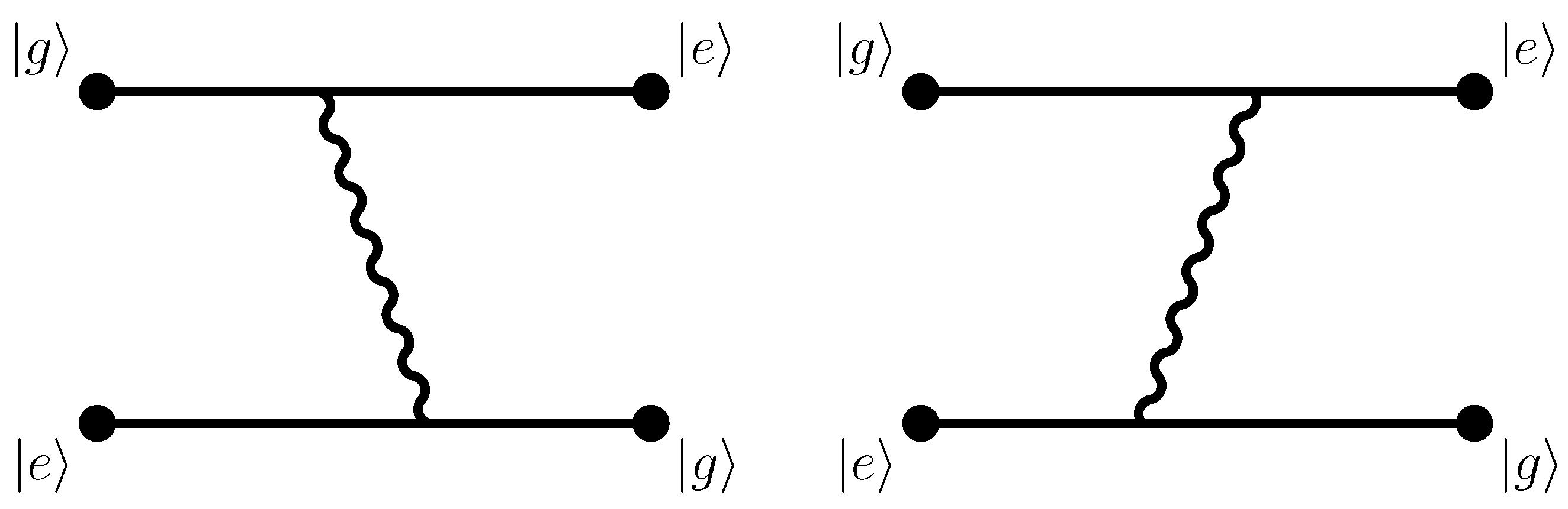
Normally, one assumes that interatomic long-range interactions (van der Waals interactions) are associated with fluctuating dipole moments of the two interacting atoms, which, in turn, are due to quantum fluctuations of the electron positions in both atoms. In the dipole approximation, the interaction Hamiltonian is equal to the scalar product of the dipole operator and the second-quantized electric-field operator. If both atoms are in an initial ground state (which is generally spherically symmetric), then both of them undergo a virtual dipole transition to an excited state during the process. One possibility for the time-ordered processes which lead to the interaction potential involves initial emission (from atom A) and absorption (by atom B) of a virtual photon. The process is complete upon the exchange of a second virtual photon, with the order of emission (from atom B) and absorption (by atom A) reversed (see diagram iv in Figure 7.5 of Ref. [1] and diagram d in Figure 5.1 of Ref. [2]. The final state has both atoms in the ground state, without any photons present (no excitations of the photon field). The energy of the final state is equal to that of the initial state, but energy conservation does not hold for the virtual transitions. In time-ordered perturbation theory, upon considering all possible time orderings of photon emissions and absorption, a total of twelve diagrams need to be considered (see Figure 7.5 of Ref. [1] and Figure 5.1 of Ref. [2]).
Because each emission and absorption of a virtual photon involves a single power of the interaction Hamiltonian, the exchange of two photons (two emissions and two absorptions) is a process of fourth-order perturbation theory. The corresponding interaction energy can be calculated in both time-ordered perturbation theory (see Ref. [1] and Chapter 5 of Ref. [2]) and by matching the scattering amplitude to the effective Hamiltonian (see Ref. [3] and Chapter 12 of Ref. [2]). The above situation pertains to two interacting ground-state atoms, and the resulting expressions contain the polarizabilities of both involved atoms. The result (for both identical as well as nonidentical ground-state atoms) smoothly interpolates between the nonretarded short-range 1 / R 6 so-called van der Waals limit and the fully retarded 1 / R 7 long-range limit of the interaction. The process involves the exchange of two virtual photons (see Ref. [1] and Chap. 5 of Ref. [2]).
However, if we consider two identical atoms, one of which is in an excited state, there can be energetically degenerate states of the two-atom system which are connected with the initial state of the process by the exchange of a single, not two, virtual photons. In the quantum-field theoretical picture, this situation corresponds to a nonvanishing transition matrix elements of the interaction Hamiltonian already in the second-order perturbation theory of the second-quantized Hamiltonian. For example, if one of the atoms (atom A) is a hydrogen atom in a 1 S state, and the other (atom B) is a hydrogen atom in a 2 P state, then there can be a one-photon exchange process which connects the initial state to a state where atom A is in the 2 P , and atom B is in the 1 S state. The final state is energetically fully degenerate with the initial state of the process. This implies that the eigenstates of the combined Hamiltonian of the individual atoms, and of the interaction, are coherent superpositions of product states of atoms A and B in the | ( 1 S ) A ( 2 P ) B , | ( 2 P ) A ( 1 S ) B states. (An illustrative discussion can also be found near the beginning of Chap. 7 of Ref. [1]).
In the nonretarded approximation, this process has been treated in Refs. [4,5,6,7]. One observes that the treatment in these references relies on the use of the van-der-Waals interaction Hamiltonian
H vdW = δ i j 3 R ^ i R ^ j d A i d B j 4 π ϵ 0 R 3 ,
which involves the product of the dipole operators of both atoms. Here, R is the interatomic separation vector, R ^ = R / R is its unit vector, δ i j is the Kronecker symbol, and d A and d B are the dipole operators for the two atoms. It leads to a nonvanishing matrix element in the energetically degenerate system in the first order of perturbation theory. One might ask how can this be understood, when we just said that one-photon exchange is a second-order perturbative process. The answer is that the van der Waals Hamiltonian is derived without field quantization, i.e., by simply expanding the electrostatic (instantaneous) Coulomb interactions of the constituent electrons and nuclei in the two atoms [4,5,6,7], in powers of the distances of the electrons and nuclei. This expansion does not use field quantization. A single nonretarded Coulomb interaction is proportional to e 2 , where e is the electron charge, and is thus of second order in the quantum-field theoretical picture, where each photon emission or absorption vertex is considered to add an order of perturbation theory. In the second-quantized picture, one uses temporal gauge (see Equation (9.133) of Ref. [2]) and describes the same process in second-order perturbation theory by using two second-quantized interaction Hamiltonians which are each proportional to the scalar product of dipole operators and second-quantized electric field. Because the dipole operators are proportional to e, the resulting interaction is also proportional to e 2 . The timelike component of the photon propagator vanishes in temporal gauge, and it is therefore ideally suited to treat the retarded form of the van der Waals interaction.
Implicitly, the temporal gauge actually is used in the derivation outlined in Chap. 7 of Ref. [1], where the interaction with the radiation field is formulated exclusively in terms of the dipole coupling term with the electric field. A decisive difference to the derivation outlined here is that, in our covariant approach, the consideration of two different time orderings of the photon emission and absorption by the two atoms involved in the interaction. Hence, by using the technique of matching the effective Hamiltonian with the scattering matrix element, we can unify both time orderings into one single Feynman diagram. The most interesting consequence of the use of the Feynman prescription is the emergence of an imaginary part of the one-photon exchange interaction, which leads to a modification of the decay rate.
The modification of the decay rate is especially interesting for two-atom Dicke states [8], otherwise known as Bell states [9], which constitute entangled states of the two-atoms system. If we denote the ground state as | ψ g and the excited state as | ψ e , then the Dicke states are
(2) | Ψ ± = 1 2 | ( ψ e ) A ( ψ g ) B ± | ( ψ g ) A ( ψ e ) B (3) = 1 2 | ψ e ψ g ± | ψ g ψ e .
Let us briefly discuss the entanglement. On the basis of states
| ψ 1 = | ψ g , | ψ 2 = | ψ e ,
one can form the following two-particle states,
| Φ 1 = | ψ g ψ g , | Φ 2 = | ψ e ψ g , | Φ 3 = | ψ g ψ e , | Φ 4 = | ψ e ψ e .
Dicke states have the form
| Ψ ± = 1 2 | Φ 2 ± 1 2 | Φ 3 = i = 1 2 j = 1 2 c i j ± | ψ i ψ j , c 12 ± = 1 2 , c 21 ± = ± c 12 ± ,
while all c i j ± other than c 12 ± and c 21 ± vanish. It is crucial to observe that these c i j cannot be written in the form c i j = a i b j , and the Dicke states are thus entangled.
As a clarifying remark, we do not consider transient phenomena connected to the excitation process [10,11,12,13,14,15,16,17], and (see also Equations (5.10), (5.11), and (5.16) of Ref. [16]) and consider the entangled Dicke states as the basis of our discussions. This paper studies the properties, not the preparation, of the entangled Dicke states. Following p. 200 of Ref. [18], we remark that the concept of an intermolecular interaction energy for the situation in which the initial state of A or B corresponds to an excited state holds as long as the excited state or states in question are sufficiently long lived relative to the time taken for the photon to propagate between the two sites. The preparation of Dicke states by carefully engineered light pulses has been discussed in Equations (4.21) and Equations (7.1), (7.2) and (7.3) of Ref. [19]. Further considerations on suitable preparation algorithms have been reported in Refs. [20,21,22]. We note that the entangled state denoted here as | Ψ + is known as the Bell state | Ψ + in the literature on quantum computation [9,19].
From a historical perspective, it is interesting to remark that the possibility of resonant energy transfer between excited and ground states of atomic and molecular systems via the exchange of resonant virtual photons has been recognized in the early days of quantum mechanics [23,24,25,26], and summarized in reviews [27,28,29]. Thus, considerable effort has been invested into the calculation of the retardation corrections to the interaction potential given in Equation (1) (see Refs. [29,30,31,32,33,34,35,36,37]).
The three advantages of the second-quantized picture are that (i) it becomes possible to study the effect of retardation, i.e., the effect of the finite speed of light is the propagation of the interaction from atom A to atom B, and (ii) it is possible to obtain precise formulas for the distance-dependent modification of the decay rate of Dicke states. Furthermore, (iii) the field-theoretical formalism employed here allows us to consistently identify the position of the poles of the propagator denominators, in view of a consistent application of the Feynman prescription [2], which is implicit in the matching procedure employed here. Our goal is to obtain the interaction potential between atoms, on account of retardation, as a function of the variable ω R / c , where ω is an angular frequency of a photon, R is the interatomic distance, and c is the speed of light.
Our calculation pertains to the exchange of one, not two, photons. In the contrasting case of the two-photon interaction, ω is the modulus of the frequency of either of the two virtual photons; the frequencies add up to zero in view of energy conservation in the initial and final states [3]. Thus, the relevant diagrams for the one-photon exchange are not those given in Figure 5.1 of Ref. [2], not those given in Figure 7.5 of Ref. [1], and not those given in Figure 1 of Ref. [38], but rather those given in Figure 1 of Ref. [33], Figure 1 of Ref. [37], and Figure 2 of Ref. [29] (and in Figure 1 here). Natural units with = c = ϵ 0 are used in the following unless stated otherwise.

2. S–Matrix and Effective Hamiltonian

It is useful to recall the principle of matching the S matrix with the effective Hamiltonian. We consider two identical atoms A and B in the initial states | g and | e (ground and excited),
ψ A ( r A ) = ψ g ( x A R A ) , E A = E g , ψ B ( r B ) = ψ e ( x B R B ) , E B = E e ,
which scatter into the final states
ψ A ( r A ) = ψ e ( x A R A ) , E A = E e , ψ B ( r B ) = ψ g ( x B R B ) , E B = E g ,
under the action of a potential U. The electron coordinates are x A and x B , and the coordinates of the nuclei are R A and R B . The energies of the states | g and | e are assumed to differ by ω 0 , where
ω 0 = | E A E B | = | E A E B | = | E e E g | .
The final state of the process has the energy of the two atomic states interchanged and therefore the same energy as the initial state. The corresponding Feynman diagrams are given in Figure 1.
For the matching, we consider the action of the potential U ( r A , r B , R ) , where R = R A R B is the interatomic distance. The corresponding (first-order) S-matrix element reads as follows:
S f i = i d 3 r A d 3 r B ψ A ( r A ) ψ B ( r B ) U ( r A , r B , R ) ψ A ( r A ) ψ B ( r B ) × d t e i ( E A + E B E A E B ) t = i T d 3 r A d 3 r B ψ A ( r A ) ψ B ( r B ) U ( r A , r B , R ) ψ A ( r A ) ψ B ( r B ) .
We have assumed energy conservation ( E A + E B = E A + E B ) and denoted the (long) time interval over which the transition from initial to final state occurs, as d t = T . In our calculations, we shall obtain the (manifestly) nonforward scattering amplitude (the final states differ from the initial states) in the functional form
S f i = i d 3 r A d 3 r B ψ A ( r A ) ψ B ( r B ) S ( r A , r B , R ) ψ A ( r A ) ψ B ( r B ) = i ψ A ψ B S ψ A ψ B .
The matching relation is thus
S ( r A , r B , R ) = T U ( r A , r B , R ) , R = R A R B .
The use of the notation S ( r A , r B , R ) indicates that we obtain the matching in the integrand of the scattering matrix element. The final integration occurs over the wave functions of the initial and final states of the two-atom system.

3. Calculation of the Effective Hamiltonian

In time-dependent quantum electrodynamic (QED) perturbation theory, the interaction is formulated in the interaction picture [2,39,40]. The second-quantized operators in the interaction Hamiltonian have a time dependence which is generated by the action of the free Hamiltonian (see Chap. 3 of Ref. [2]). The designation of an interaction Hamiltonian being formulated in the interaction picture is not redundant (see Chap. 3 of Ref. [2]). The interaction Hamiltonian is
V ( t ) = E ( R A , t ) · d A ( t ) E ( R B , t ) · d B ( t ) .
Here, d k = e r k = e ( x k R k ) with k = A , B is the dipole operator for atom k (for atoms with more than one electron, one has to sum over all the electrons). The R A and R B are the positions of the atomic nuclei, whereas the x A and x B denote the electron coordinates. The second-order contribution to the S-matrix is
ϕ , 0 | S ( 2 ) | ϕ , 0 = ( i ) 2 2 ! d t 1 d t 2 ϕ , 0 T [ V ( t 1 ) V ( t 2 ) ] ϕ , 0 .
Here, T denotes the ordering of all operators, pertaining to both atomic dipoles and electric fields. We denote by | 0 the “vacuum” of the electromagnetic field. In the vacuum, there are no photons in the radiation field. Let us also denote the initial state as | ϕ   =   | ψ A = ψ g , ψ B = ψ e and the final two-atom state as | ϕ   =   | ψ A = ψ e , ψ B = ψ g , with the conditions given in Equations (7) and (8). Then,
ϕ , 0 T [ V ( t 1 ) V ( t 2 ) ] ϕ , 0 = ϕ , 0 T E ( R A , t 1 ) · d A ( t 1 ) E ( R B , t 1 ) · d B ( t 1 ) × E ( R A , t 2 ) · d A ( t 2 ) E ( R B , t 2 ) · d B ( t 2 ) ϕ , 0 ϕ , 0 T E ( R A , t 1 ) · d A ( t 1 ) E ( R B , t 2 ) · d B ( t 2 ) ϕ , 0 + ϕ , 0 T E ( R B , t 1 ) · d B ( t 1 ) E ( R A , t 2 ) · d A ( t 2 ) ϕ , 0 ,
where by ∼ we denote the omission of operators which pertain to the one-loop self energy of the two atoms, and keep only the terms relevant for the interaction energy. The time ordering of the electric field operators and atomic dipole operators leads to
S ( 2 ) = 1 2 d t 1 d t 2 0 T E i ( R A , t 1 ) E j ( R B , t 2 ) 0 ψ e ψ g T d A i ( t 1 ) d B j ( t 2 ) ψ g ψ e 1 2 d t 1 d t 2 0 T E i ( R B , t 1 ) E j ( R A , t 2 ) 0 ψ e ψ g T d B i ( t 1 ) d A j ( t 2 ) ψ g ψ e .
Here, T is the time ordering operator for the atomic dipole moments, and the T operator time-orders the electric field operators. Moreover, i , j = 1 , 2 , 3 denote the Cartesian components. We use a relativistic notation where the superscript denotes the Cartesian component.
We now recall a few known results from Ref. [3] and Chap. 12 of [2]. The time-ordered product of electric-field operators can be evaluated as follows:
0 T E i ( R A , t 1 ) E j ( R B , t 2 ) 0 = i d ω 2 π ω 2 D F i j ( ω , r ) e i ω ( t 1 t 2 ) .
Here, in agreement with Equation (85.15) of Ref. [41],
D F i j ( ω , R ) = δ i j + i j ω 2 e i | ω | R 4 π R , | ω | = ω 2 + i ϵ
is the photon propagator in the mixed frequency-position representation, in the temporal gauge (in the conventions outlined in Equation (9.133) of Ref. [2]). In the temporal gauge, the timelike component of the photon propagator vanishes, and one has D 00 ( ω , R ) = 0 . We use the photon propagator in the convention i D F μ ν ( x x ) = 0 T A μ ( x ) A ν ( x ) 0 , with μ , ν = 0 , 1 , 2 , 3 , where A μ ( x ) is the quantized four-vector potential propagator. The result for the spatial components of the photon propagator is found according to Refs. [3,42],
D F i j ( ω , R ) = α i j + β i j i | ω | R 1 ω 2 R 2 e i | ω | R 4 π R , α i j = δ i j R ^ i R ^ j , β i j = δ i j 3 R ^ i R ^ j ,
where | ω | = ω 2 + i ϵ , and the branch cut of the square root is taken along the positive real axis [43,44]. Now, let us proceed to evaluate the time-ordered product of dipole operators,
X i j ( t 1 t 2 ) = ψ e ψ g T d A i ( t 1 ) d A j ( t 2 ) ψ g ψ e = ψ e ψ g T d A i ( t 1 t 2 ) d A j ( 0 ) ψ g ψ e .
Introducing the Fourier transform X i j ( ω ) , we can write X i j ( t 1 t 2 ) = d ω 2 π e i ω ( t 1 t 2 ) X i j ( ω ) . The Fourier transform of the time-ordered product of dipole operators can be evaluated as follows:
X i j ( ω ) = d t e i ω t X i j ( t ) = d t e i ω t ψ e ψ g T d A i ( t ) d B j ( 0 ) ψ g ψ e = 0 d t e i ω t ψ e ψ g d A i ( t ) d B j ( 0 ) ψ g ψ e + 0 d t e i ω t ψ e ψ g d B j ( 0 ) d A i ( t ) ψ g ψ e = 0 + 0 d t e i ω t ψ e d A i ( t ) ψ g ψ g d B j ( 0 ) ψ e .
We have used the fact that the atoms are identical and undergo transitions | g | e and | e | g , respectively. We can thus add the two integration domains and conclude that
X i j ( ω ) = d t e i ω t ψ e d A i ( t ) ψ g ψ g d B j ( 0 ) ψ e = d t e i ω t e i ( E 2 E 1 ) t ψ e d A i ( 0 ) ψ g ψ g d B j ( 0 ) ψ e = 2 π δ ( E 2 E 1 + ω ) ψ e d A i ( 0 ) ψ g ψ g d B j ( 0 ) ψ e .
The two terms in Equation (16) yield equivalent contributions, and we obtain, with the help of the results obtained previously for the time-ordered products of the electric-field and atomic dipole operators,
S ( 2 ) = 1 2 d t 1 d t 2 0 T E i ( R A , t 1 ) E j ( R B , t 2 ) 0 ψ e ψ g T d A i ( t 1 ) d B j ( t 2 ) ψ g ψ e = d t 1 d t 2 i d ω 2 π ω 2 D F i j ( ω , R ) e i ω ( t 1 t 2 ) e i ( E 1 E 2 ) ( t 1 t 2 ) × ψ e d A i ψ g ψ g d B j ψ e = i d ( t 1 t 2 ) d t 2 d ω 2 π ω 2 D F i j ( ω , R ) e i ( ω + E 1 E 2 ) ( t 1 t 2 ) ψ e d A i ψ g ψ g d B j ψ e = i T ( E 2 E 1 ) 2 D F i j ( | E 2 E 1 | , R ) ψ e ψ g d A i d B j ψ g ψ e ,
where d A i d A i ( 0 ) and d B j d B j ( 0 ) . Based on the matching relation (12) and remembering Equation (9), we read off the interaction potential,
U ( r A , r B , R ) = ( E 2 E 1 ) 2 D i j ( | E 2 E 1 | , R ) d A i d B j = ω 0 2 α i j + β i j i ω 0 R 1 ω 0 2 R 2 e i ω 0 R 4 π R d A i d B j = δ i j 3 R i R j R 2 1 i ω 0 R δ i j R i R j R 2 ω 0 2 R 2 e i ω 0 R 4 π R 3 d A i d B j .
This result confirms results previously obtained in Equations (13), (14) and (40)–(42) of Ref. [31], Equations (12)–(14) of Ref. [33], Equation (2.23) of Ref. [34], Equations (4) and (5) of Ref. [35], Equation (2.1) of Ref. [36], Equations (3.5)–(3.7) of Ref. [32], Equation (14) of Ref. [37], and Equation (5) of Ref. [29]. One important advantage of the method of derivation employed here is that the imaginary part follows directly from the Feynman prescription for the propagator denominators. In other approaches, additional considerations are required to fix the location of the poles of the propagators in the complex plane (for an illustrative discussion on this point, see Ref. [29]). This potential can be separated into a real and an imaginary part,
Re [ U ( r A , r B , R ) ] = β i j cos ( ω 0 R ) + ω 0 R sin ( ω 0 R ) α i j ω 0 2 R 2 cos ( ω 0 R ) d A i d B j 4 π R 3 ,
Im [ U ( r A , r B , R ) ] = β i j sin ( ω 0 R ) ω 0 R cos ( ω 0 R ) α i j ω 0 2 R 2 sin ( ω 0 R ) d A i d B j 4 π R 3 .
The real part had previously been given in Equation (5) of Ref. [30] and in Equation (7.2.27) on page 149 in Chapter 7 of Ref. [1]. We have used the relations given in Equation (19). By using R ^ = R / R , one has the static limit ( ω 0 R 0 ),
U ( r A , r B , R ) δ i j 3 R ^ i R ^ j d A i d B j 4 π R 3 ω 0 0 ,
which verifies the well-known expression for the nonretarded van der Waals interaction given in Equation (1). SI units can be restored by multiplication with an additional overall factor 1 / ϵ 0 , and replacing the factor ω 0 R by the (dimensionless) factor ω 0 R / c .

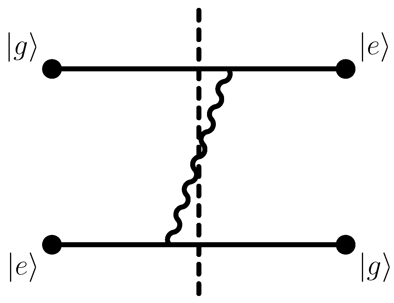
4. Interpretation of the Imaginary Part

The imaginary part of the interatomic interaction potential given in Equation (25b) is oscillating in sign. It describes the one-photon resonant emission from the decaying excited state which forms part of the entangled Dicke states given in Equation (2). In full analogy, the imaginary part of the one-loop self-energy of an excited bound state in atom is naturally interpreted in terms of the decay width of that same excited reference state [45,46,47]. The corresponding Feynman diagram is given in Figure 2. The atomic ground state is a valid final state for the decay process (see also Figure 1 of Ref. [32], Section 2.1 of Ref. [35] and Ref. [34]). However, as we have seen, the sign of the imaginary part of the exchange interaction potential given in Equation (25b) is oscillating. For a decay rate to be described by the imaginary part of an energy shift, we would not expect such an oscillation; hence, a careful interpretation is required. Indeed, the oscillating character of the imaginary part could be seen as a problem because the imaginary part of the resonance energy of a decaying state is required to be negative [48,49]; a positive imaginary part would correspond to an antiresonance and a negative decay rate. The solution is presented in the following. We can anticipate that the negative decay rate, which could otherwise naively result from the interaction energy, is compensated by the natural decay rate, to give the subradiant and superradiant states their (nonnegative) decay rates.
One generally writes a resonance energy in terms of Re E i Γ / 2 , where Γ is the width. Hence, it is useful to define a decay rate operator Γ ^ ( ξ ) , where ξ = ω 0 R is the dimensionless argument appearing in Equation (25b). This operator is related to the imaginary part of the exchange potential as follows:
Γ ^ ( ξ ) = 2 Im [ U ( r A , r B , R ) ] , ξ = ω 0 R .
We write the result given in Equation (25b) somewhat differently, as
Γ ^ ( ξ ) = 3 2 ξ cos ( ξ )   +   [ ξ 2 1 ] sin ( ξ ) ξ 3 4 α 3 ω 0 3 δ i j R i R j R 2 r A i r B j +   3 sin ( ξ )     ξ cos ( ξ ) ξ 3 4 α 3 ω 0 3 R i R j R 2 r A i r B j .
This expression can be conveniently written in terms of a transverse decay operator Γ ^ ( ξ ) , which describes a transition whose polarization axis is perpendicular to the interatomic distance vector R , and a longitudinal decay operator Γ ^ ( ξ ) , which describes transition whose polarization axis is parallel to the interatomic distance vector R . The result is
Γ ^ ( ξ ) = Γ ^ ( ξ ) + Γ ^ ( ξ ) , Γ ^ ( ξ ) = f ( ξ ) Γ ^ ( 0 ) , Γ ^ ( ξ ) = f ( ξ ) Γ ^ ( 0 ) .
The weight functions f ( ξ ) and f ( ξ ) and the transverse and longitudinal decay operator at zero distance, Γ ^ ( 0 ) and Γ ^ ( 0 ) , are given as follows:
Γ ^ ( 0 ) = 4 α 3 ω 0 3 δ i j R i R j R 2 r A i r B j ,
Γ ^ ( 0 ) = 4 α 3 ω 0 3 R i R j R 2 r A i r B j ,
Γ ^ ( 0 ) = Γ ^ ( 0 ) + Γ ^ ( 0 ) = 4 α 3 ω 0 3 δ i j r A i r B j ,
f ( ξ ) = 3 ξ cos ( ξ ) + [ ξ 2 1 ] sin ( ξ ) 2 ξ 3 = 1 + O ( ξ 2 ) ,
f ( ξ ) = 3 sin ( ξ ) ξ cos ( ξ ) ξ 3 = 1 + O ( ξ 2 ) .
Here, Γ ^ ( 0 ) is the total decay operator at zero distance. It fulfills the relation ψ e ψ g | Γ ^ ( 0 ) | ψ g ψ e = Γ ( 0 ) , where Γ ( 0 ) (no hat symbol over the Γ ) is the natural decay width of the excited state in vacuum, which is obtained without consideration of the atom–atom interaction and its consequential modification of the decay rate. One compares it with Equation (3.37) of Ref. [2].
Let us now investigate the two Dicke states:
| Ψ ± = 1 2 | ψ e ψ g ± | ψ g ψ e .
The expectation value of the decay rate operator can be written as follows:
(36) Ψ ± | Γ ^ ( ξ ) | Ψ ± = ± ψ g ψ e | Γ ^ ( ξ ) | ψ e ψ g (37) = ± f ( ξ ) Γ e g ( 0 ) + f ( ξ ) Γ e g ( 0 ) .
Here,
(38) Γ e g ( 0 ) = ψ g ψ e | Γ ^ ( 0 ) | ψ e ψ g = 4 α 3 ω 0 3 δ i j R i R j R 2 g | r A i | e e | r B j | g (39) = 4 α 3 ω 0 3 δ i j R i R j R 2 g | r A i | e e | r A j | g ,
(40) Γ e g ( 0 ) = ψ g ψ e | Γ ^ ( 0 ) | ψ e ψ g = 4 α 3 ω 0 3 R i R j R 2 g | r A i | e e | r B j | g (41) = 4 α 3 ω 0 3 R i R j R 2 g | r A i | e e | r A j | g ,
Γ ( 0 ) = Γ e g ( 0 ) + Γ e g ( 0 ) = 4 α 3 ω 0 3 | g | r A | e | 2 .
We have repeatedly used the fact that the two atoms are identical to replace r B j r A j . Note that Γ e g ( 0 ) and Γ e g ( 0 ) can depend on the magnetic projections, but the natural width Γ ( 0 ) is independent of magnetic quantum numbers [2].
In the space spanned by the | ψ g ψ e and | ψ e ψ g , one finally obtains the following effective Hamiltonian for the two-atoms system, which takes into account the one-photon exchange and, with it, the imaginary part of the exchange energy,
H = E g + E e i 2 Γ ( 0 ) | ψ g ψ e ψ g ψ e | + | ψ e ψ g ψ e ψ g | + | ψ g ψ e Re U ( ξ ) i 2 f ( ξ ) Γ ( 0 ) + f ( ξ ) Γ ( 0 ) ψ e ψ e | + h . c . .
Here, E e = Re E e is the real part of the energy of the excited state, and we have supplemented the term i Γ ( 0 ) / 2 in the resonance energy of the unperturbed states. It means that in the basis of states | ψ g ψ e , | ψ e ψ g , the Hamiltonian matrix is
H = E 0 δ E δ E E 0 , E 0 = E g + E e i 2 Γ ( 0 ) , δ E = E γ i 2 Γ γ .
Here,
E γ = ψ g ψ e | Re U ( ξ ) | ψ g ψ e , Γ γ = ψ g ψ e | Γ ^ ( ξ ) | ψ g ψ e ,
describe the real and imaginary parts of the one-photon exchange energy. We write the vector representation of the Dicke states | Ψ and | Ψ + and E = E ( ξ ) , and E + = E + ( ξ ) , as follows:
| Ψ ± = 1 2 1 ± 1 , E ± = E 0 ± δ E .
The resonance energies can be written as follows:
E ( R ) = Re E 0 + E γ i 2 Γ ( 0 ) f ( ξ ) Γ e g ( 0 ) + f ( ξ ) Γ e g ( 0 ) ,
E + ( R ) = Re E 0 E γ i 2 Γ ( 0 ) + f ( ξ ) Γ e g ( 0 ) + f ( ξ ) Γ e g ( 0 ) .
The effective decay rates of the Dicke states are
Γ ( R ) = Γ ( 0 ) f ( ξ ) Γ e g ( 0 ) + f ( ξ ) Γ e g ( 0 ) = O ( ξ 2 ) ,
Γ + ( R ) = Γ ( 0 ) + f ( ξ ) Γ e g ( 0 ) + f ( ξ ) Γ e g ( 0 ) = 2 Γ ( 0 ) O ( ξ 2 ) .
Hence, | Ψ is the entangled subradiant state, and | Ψ + is the superradiant state. In the short-range limit, the subradiant state | Ψ becomes metastable in view of the entanglement, whereas the superradiant state | Ψ + acquires twice the natural decay width.

5. Verification of the Result

Let us include some cryptic remarks regarding a verification of the results given in Equations (49) and (50) based on an alternative method. To this end, one considers Equation (7.2.4) of Ref. [1], but crucially takes into account that the entangled photon emissions from the atoms A and B happen at different positions. Thus, one considers the matrix element M,
M = 1 2 ψ g ψ g ϵ ^ · r A e i k · R A + ϵ ^ · r B e i k · R B ψ e ψ g ± ψ g ψ e 2 = ψ g ϵ ^ · r A ψ e 2 ± ψ g ϵ ^ · r A ψ e 2 cos ( k · R ) ,
where R = R A R B . In the last step, we have used the indistinguishability of the two identical atoms. Furthermore, on resonance, one has | k | = ω 0 . The sum over the two photon polarizations results in
λ ϵ λ i ϵ λ j = δ i j k i k j k 2 .
After some algebra, one shows the result
d Ω 3 8 π δ i j k i k j k 2 cos ( ω 0 k ^ · R ) = δ i j R i R j R 2 f ( ω 0 R ) + R i R j R 2 f ( ω 0 R ) ,
where the previously obtained weight functions f ( ω 0 R ) and f ( ω 0 R ) (see Equations (33) and (34)) naturally appear. Based on these identities and the formalism outlined in Chaps. 3 and 4 of Ref. [2], one can verify the results given in Equations (49) and (50). The first term on the right-hand side of Equation (53) gives the term Γ ( 0 ) in Equations (49) and (50), whereas the second term on the right-hand side of Equation (53) gives the second term on the right-hand side of Equations (49) and (50).
Conversely, the introduction of the Feynman prescription into the formalism outlined in Ref. [1], which was initially designed to obtain the real part of the resonant one-photon exchange interaction only, leads to the imaginary part obtained here. Notes on this point are collected in the Appendix A.

6. Example of Superradiant and Subradiant States

We would like to conclude this work with a concrete example, namely, the hydrogen atom, wherein the 1 S state is the ground state and the excited state could be one of three 2 P states, which we take on a Cartesian basis. Furthermore, we assume that the interatomic distance is along the z axis,
R = R e ^ z .
The wave functions are well known:
ψ g ( r ) = ψ 1 S ( r ) = 1 π a 0 3 / 2 exp r a 0 , r = | r | ,
ψ e , x ( r ) = ψ 2 P , x ( r ) = r sin θ cos φ 4 2 π a 0 5 / 2 exp r 2 a 0 ,
ψ e , y ( r ) = ψ 2 P , y ( r ) = r sin θ sin φ 4 2 π a 0 5 / 2 exp r 2 a 0 ,
ψ e , z ( r ) = ψ 2 P , z ( r ) = r cos θ 4 2 π a 0 5 / 2 exp r 2 a 0 .
The nonvanishing dipole transition matrix elements are as follows:
ψ g | x | ψ e , x = ψ g | y | ψ e , y = ψ g | z | ψ e , z = 2 7 3 5 2 a 0 ,
and all other combinations vanish (e.g., ψ g | x | ψ e , y = 0 ). The resonance frequency is
ω 0 = 3 8 α 2 m ,
and the natural decay width is (see Ref. [51])
Γ ( 0 ) = 2 8 3 8 α 5 m ,
where α is the fine structure constant. The x and y polarized P states cannot decay via a z-polarized transition, and the z polarized P states decay exclusively via a z-polarized transition. We have the results
Γ 0 x ( 0 ) = Γ 0 y ( 0 ) = Γ 0 z ( 0 ) = Γ ( 0 ) , Γ 0 x ( 0 ) = Γ 0 y ( 0 ) = 0 , Γ 0 z ( 0 ) = 0 .
One can thus define the distance-dependent transverse and longitudinal decay rates, Γ ( ξ ) and Γ ( ξ ) ,
Γ ( ξ ) = Γ 0 x ( ξ ) = Γ 0 y ( ξ ) = f ( ξ ) Γ ( 0 ) ,
Γ ( ξ ) = Γ 0 z ( ξ ) = f ( ξ ) Γ ( 0 ) , ξ = ω 0 R .
At short range, the decay-rate admixtures expand as follows:
Γ ( R ) Γ ( 0 ) = 1 ( ω 0 R ) 2 5 + O ( ( ω 0 R ) 4 ) ,
Γ ( R ) Γ ( 0 ) = 1 ( ω 0 R ) 2 10 + O ( ( ω 0 R ) 4 ) .
From the x or y polarized P states, we have the following subradiant entangled Dicke states:
| Ψ x = 1 2 ( | ψ g ψ e , x | ψ e , x ψ g ) , | Ψ y = 1 2 ( | ψ g ψ e , y | ψ e , y ψ g ) .
They have the following decay rates:
(65) Γ ( R ) = Γ ( 0 ) Γ ( R ) = Γ ( 0 ) [ 1 f ( ξ ) ] (66) = Γ ( 0 ) × ( ω 0 R ) 2 5 + O ( ( ω 0 R ) 4 ) ω 0 R 0 1 3 sin ( ω 0 R ) 2 ω 0 R + O 1 ( ω 0 R ) 2 ω 0 R .
In the short-range limit, the decay is suppressed, whereas in the long-range limit, the natural decay width is approached, albeit with a long-range, sinusoidal modification. For the z polarized (longitudinal), subradiant state,
| Ψ = 1 2 ( | ψ g ψ e , z | ψ e , z ψ g ) ,
one finds for the decay rate
(68) Γ ( R ) = Γ ( 0 ) Γ ( R ) = Γ ( 0 ) [ 1 f ( ξ ) ] (69) = Γ ( 0 ) × ( ω 0 R ) 2 10 + O ( ( ω 0 R ) 4 ) ω 0 R 0 1 + 3 cos ( ω 0 R ) ( ω 0 R ) 2 + O 1 ( ω 0 R ) 4 ω 0 R .
From the x or y polarized P states, we calculate the following superradiant entangled Dicke states:
| Ψ + x = 1 2 ( | ψ g ψ e , x + | ψ e , x ψ g ) , | Ψ + y = 1 2 ( | ψ g ψ e , y + | ψ e , y ψ g ) .
One finds the decay rates
(71) Γ + ( R ) = Γ ( 0 ) + Γ ( R ) = Γ ( 0 ) [ 1 + f ( ξ ) ] (72) = Γ ( 0 ) × 2 ( ω 0 R ) 2 5 + O ( R 4 ) ω 0 R 0 1 + 3 sin ( ω 0 R ) 2 ω 0 R + O 1 ( ω 0 R ) 2 ω 0 R .
In the short-range limit, the decay rate is twice the natural width, whereas in the long-range limit the natural width is approached with a long-range sinusoidal modification. One also finds the following superradiant longitudinal entangled Dicke state:
| Ψ + = 1 2 ( | ψ g ψ e , z + | ψ e , z ψ g ) .
The distance-dependent decay rate is
(74) Γ + ( R ) = Γ ( 0 ) + Γ ( R ) Γ ( 0 ) χ + ( ω 0 R ) (75) = Γ ( 0 ) × 2 ( ω 0 R ) 2 10 + O ( ( ω 0 R ) 4 ) ω 0 R 0 1 3 cos ( ω 0 R ) ( ω 0 R ) 2 + O 1 ( ω 0 R ) 3 ω 0 R .
The results are illustrated in Figure 3 and Figure 4.

7. Brief Summary and Conclusions

We have considered retardation corrections to the resonant one-photon exchange between identical atoms, one of which is in an excited state. In Section 2, we have considered the matching of the S matrix element and the effective Hamiltonian. Specifically, our calculations have been based on the nonforward-scattering matrix element induced by an interaction potential of the functional form U ( r A , r B , R ) , which depends on the relative coordinates r A and r B of the two atoms, and the interatomic distance R . For the matching to be successful, we need to assume the initial and final states of the process to have identical energy. This is the case if, e.g., the initial state is a combination of one of the atoms in the ground state, and the other atom in an excited P state. The final state has the energies of the two states reversed. Because the energies of the quantum states of the individual states have been exchanged in the initial and final states of the identical atoms, the total energy of the final state is equal to that of the initial state, and the matching of the nonforward S matrix element to the effective Hamiltonian can proceed.
This program is realized in Section 3, where the calculation is carried out in the temporal gauge for the virtual photon. In this gauge, the timelike component of the photon propagator vanishes, which implies that it is the ideal gauge for the calculation of the retardation corrections to the van der Waals potential given in Equation (1). The final result is given in Equation (24). The retarded potential has both a real and an imaginary part. The interpretation of the imaginary part of the resonant one-photon exchange energy is discussed in Section 4 and Section 5. It is found that a completely consistent picture is obtained when one calculates the Hamiltonian matrix including the unperturbed resonance energies of the ground and excited states, as well as the one-photon resonant exchange energy and its imaginary part. The modification of the decay rate of entangled Dicke states (Bell states) is consistently obtained, and the result allows us to obtain consistent formulas for the distance-dependent decay rates of the superradiant and subradiant Dicke states. An example calculation involving hydrogen 1 S and 2 P states is given in 
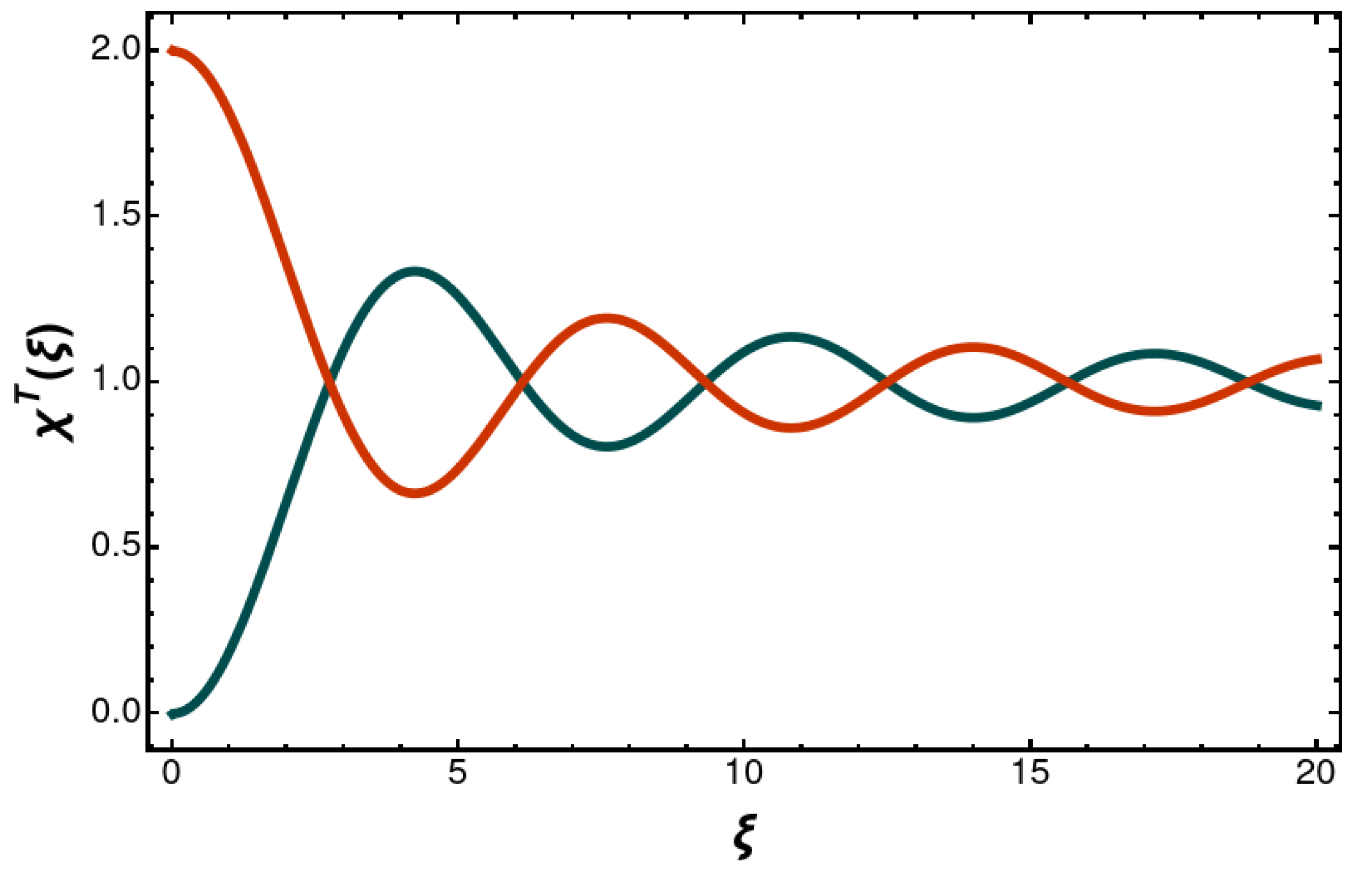
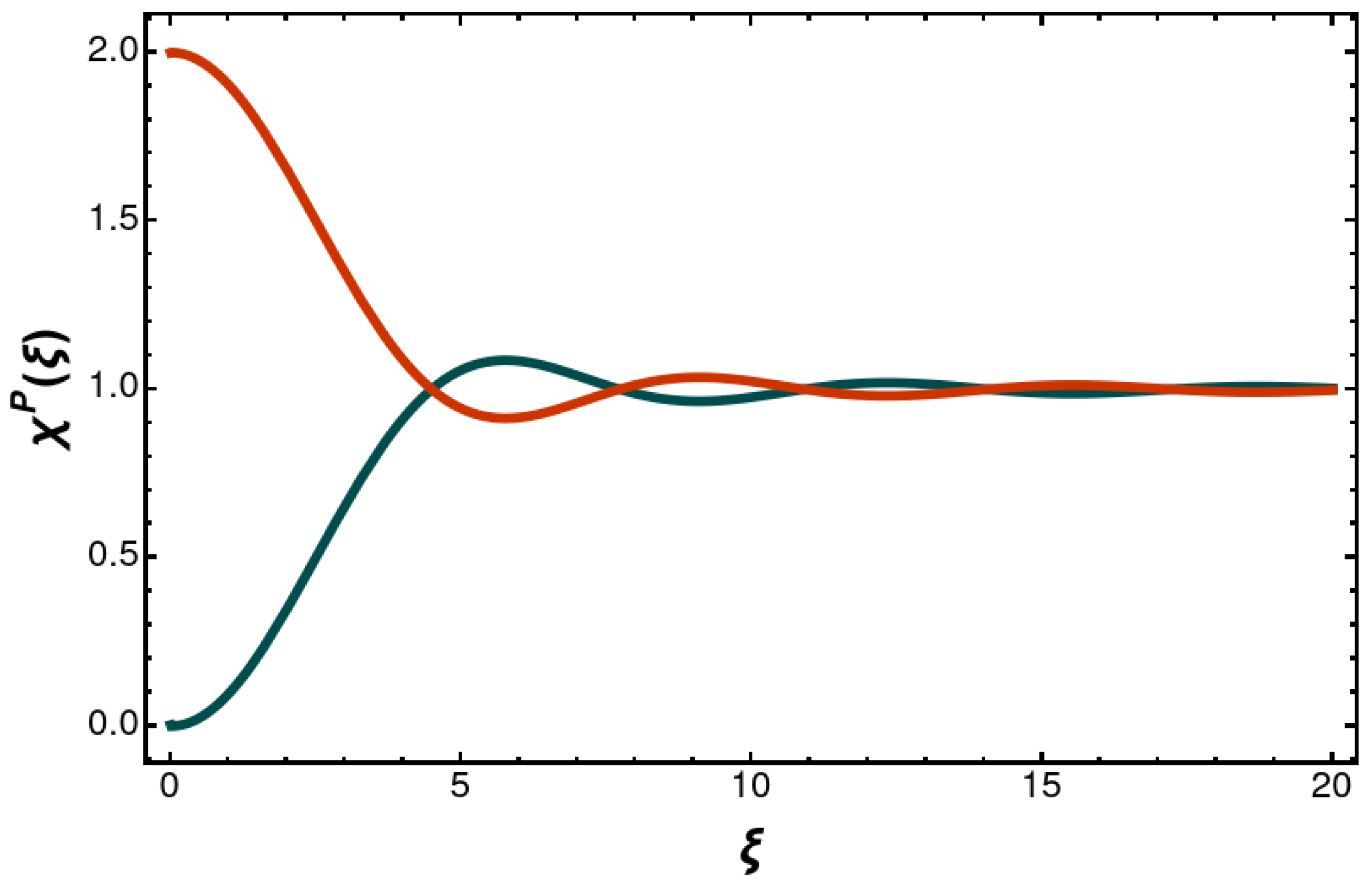
Section 6, culminating in the results presented in Figure 3 and Figure 4. The modification of the decay rates has a long-range, 1 / R tail. The imaginary part of the retarded one-photon exchange as obtained by the Feynman prescription finds an interpretation in terms of the distance-dependent entangled decay rate.

Author Contributions

U.D.J.: conceptualization; investigation; writing of the paper; C.M.A.: investigation; verification and checking of calculations. All authors have read and agreed to the published version of the manuscript.

Funding

This research was funded by the National Science Foundation (grant PHY-2110294).

Data Availability Statement

Not applicable. No experimental data involved.

Acknowledgments

The authors acknowledge helpful conversations with István Nándori.

Conflicts of Interest

The authors declare no conflict of interest.

Appendix A. Comparison with the Literature

In Chap. 7 of Ref. [1], the authors carry out a related calculation by using time-ordered perturbation theory. Specifically, in Equation (7.2.21) of Ref. [1], the authors obtain an expression for the retarded van der Waals interaction which, in our notation, reads as follows:
U ( r A , r B , R ) = lim γ 0 + 1 2 π 2 0 d p p 4 τ i j ( p R ) ω 0 2 p 2 e γ p ,
τ i j ( p R ) = α i j sin ( p R ) p R + β i j cos ( p R ) p 2 R 2 sin ( p R ) p 3 R 3 .
For clarity, we observe that ω 0 is denoted as k in Ref. [1], and that ϵ 0 is explicitly written out in Ref. [1]. In Chap. 7 of Ref. [1], the authors evaluate the integral over p as a principal-value integral by using a convergent factor, and obtain the real part of our result:
U ( r A , r B , R ) = Re [ U ( r A , r B , R ) ] .
The Feynman prescription of quantum electrodynamics is implemented by the substitution
τ i j ( p R ) ω 0 2 p 2 τ i j ( p R ) ω 0 2 p 2 + i ϵ = τ i j ( p R ) ( ω 0 + i ϵ p ) ( ω 0 + i ϵ + p )
in Equation (A1). As a function of p, the integrand then obtains poles in the complex p plane at p = ± ω 0 2 + i ϵ , i.e., at p = ω 0 + i ϵ and at p = ω 0 i ϵ , where ϵ denotes an infinitesimal positive imaginary part. In order to consider the contribution from the pole, one symmetrizes the integral on the domain < p < , and inserts the infinitesimal imaginary part, leading to
U ( r A , r B , R ) = lim ϵ 0 + lim γ 0 + 1 4 π 2 d p p 4 τ i j ( p R ) ω 0 2 p 2 + i ϵ e γ | p | .
The real part of U ( r A , r B , R ) can be evaluated by principal value, confirming the result given in Equation (A3). The imaginary part is obtained by considering the pole at p = ω 0 + i ϵ which is encircled in the mathematically positive sense,
i Im U ( r A , r B , R ) = 2 π i Res p = ω 0 1 4 π 2 p 4 τ i j ( p R ) ω 0 2 p 2 = i 4 π ω 0 3 τ i j ( ω 0 R ) = i Im U ( r A , r B , R ) ,
where the latter equality is obvious by inspection of Equations (A2), (A5) and (25b). We conclude that, if the infinitesimal imaginary part of the photon is supplemented in the treatment outlined in Chap. 7 of Ref. [1], then the result for the interaction potential U given in Equation (24) can be obtained,
U ( r A , r B , R ) = U ( r A , r B , R ) .
We should also briefly discuss certain approximations underlying our treatment that are discussed in Chap. 7 of Ref. [1]. First, we note the Born–Oppenheimer approximation, which allows us to consider the motion of the electrons and nuclei separately and corresponds to the limit of infinitely heavy atomic nuclei (vanishing electron–nucleon mass ratio). In the same light, we neglect the recoil energy upon photon emission, and we assume that the wave functions of the two atoms do not overlap. Higher-order multipoles as well as multiphoton transitions are also neglected. The same approximations underlie the treatments given in Refs. [52,53] for systems consisting of unlike atoms with close excitation energies.

References

  1. Craig, D.P.; Thirunamachandran, T. Molecular Quantum Electrodynamics; Dover Publications: Mineola, NY, USA, 1984. [Google Scholar]
  2. Jentschura, U.D.; Adkins, G.S. Quantum Electrodynamics: Atoms, Lasers and Gravity; World Scientific: Singapore, 2022. [Google Scholar]
  3. Jentschura, U.D.; Debierre, V. Long-range tails in van der Waals interactions of excited-state and ground-state atoms. Phys. Rev. A 2017, 95, 042506. [Google Scholar] [CrossRef] [Green Version]
  4. Jonsell, S.; Saenz, A.; Froelich, P.; Forrey, R.C.; Côté, R.; Dalgarno, A. Long-range interactions between two 2s excited hydrogen atoms. Phys. Rev. A 2002, 65, 042501. [Google Scholar] [CrossRef]
  5. Jentschura, U.D.; Adhikari, C.M. Long–Range Interactions for Hydrogen: 6P–1S and 6P–2S Systems. Atoms 2017, 5, 48. [Google Scholar] [CrossRef] [Green Version]
  6. Adhikari, C.M.; Debierre, V.; Matveev, A.; Kolachevsky, N.; Jentschura, U.D. Long-range interactions of hydrogen atoms in excited states. I. 2S–1S interactions and Dirac–δ perturbations. Phys. Rev. A 2017, 95, 022703. [Google Scholar] [CrossRef] [Green Version]
  7. Jentschura, U.D.; Debierre, V.; Adhikari, C.M.; Matveev, A.; Kolachevsky, N. Long-range interactions of excited hydrogen atoms. II. Hyperfine-resolved 2S–2S system. Phys. Rev. A 2017, 95, 022704. [Google Scholar] [CrossRef] [Green Version]
  8. Dicke, R.H. Coherence in Spontaneous Radiation Processes. Phys. Rev. 1953, 93, 99–110. [Google Scholar] [CrossRef] [Green Version]
  9. WikiPedia Article on Bell states. Available online: https://en.wikipedia.org/wiki/Bell_state (accessed on 20 December 2022).
  10. Milonni, P.W.; Knight, P.K. Retardation in the resonant interaction of two identical atoms. Phys. Rev. A 1974, 10, 1096–1108. [Google Scholar] [CrossRef]
  11. Biswas, A.K.; Compagno, G.; Palma, G.M.; Passante, R.; Persico, F. Virtual photons and causality in the dynamics of a pair of two-level atoms. Phys. Rev. A 1990, 42, 4291–4301. [Google Scholar] [CrossRef]
  12. Plotzke, O.; Mille, U.; Hippler, R.; Lutz, H.O. Behavior of the Polarization of Electric-Field-Induced Lyman-a Radiation. Phys. Rev. Lett. 1990, 65, 2982–2985. [Google Scholar] [CrossRef]
  13. Hegerfeldt, G.C. Causality Problems for Fermi’s Two–Atom System. Phys. Rev. Lett. 1994, 72, 596–599. [Google Scholar] [CrossRef]
  14. Milonni, P.W.; James, D.F.V.; Fearn, H. Photodetection and causality in quantum optics. Phys. Rev. A 1995, 52, 1525. [Google Scholar] [CrossRef] [PubMed]
  15. Berman, P.R.; Dubetsky, B. Causality in the excitation exchange between identical atoms. Phys. Rev. A 1997, 55, 4060–4069. [Google Scholar] [CrossRef]
  16. Power, E.A.; Thirunamachandran, T. Analysis of the causal behavior in energy transfer between atoms. Phys. Rev. A 1997, 56, 3395–3408. [Google Scholar] [CrossRef] [Green Version]
  17. Berman, P.R. Interaction energy of nonidentical atoms. Phys. Rev. A 2015, 91, 042127. [Google Scholar] [CrossRef]
  18. Salam, A. Molecular Quantum Electrodynamics; Wiley: Hoboken, NJ, USA, 2010. [Google Scholar]
  19. Riebe, M. Preparation of Entangled States and Quantum Teleportation with Atomic Qubits. Ph.D. Dissertation, Leopold-Franzens-University Innsbruck, Innsbruck, Austria, 2005. Unpublished Work. [Google Scholar]
  20. Riebe, M.; Monz, T.; Kim, K.; Villar, A.S.; Schindler, P.; Chwalla, M.; Hennrich, M.; Blatt, R. Deterministic entanglement swapping with an ion-trap quantum computer. Nat. Phys. 2008, 4, 839–842. [Google Scholar] [CrossRef]
  21. Hume, D.B.; Chou, C.W.; Rosenband, T.; Wineland, D.J. Preparation of Dicke states in an ion chain. Phys. Rev. A 2009, 80, 052302. [Google Scholar] [CrossRef] [Green Version]
  22. Bärtschi, A.; Eidenbenz, S. Deterministic Preparation of Dicke States. In Fundamentals of Computation Theory, Proceedings of the 22nd International Symposium “FCT 2019”, Copenhagen, Denmark, 12–14 August 2019; Lecture Notes in Computer Science; Ga̧sieniec, L.A., Jansson, J., Levcopoulos, C., Eds.; Springer: Cham, Switzerland, 2020; Volume 11651, pp. 126–139. [Google Scholar]
  23. Cario, G.; Franck, J. Über die Zerlegung von Wasserstoffmolekülen durch angeregte Quecksilberatome. Z. Phys. 1922, 11, 161–166. [Google Scholar] [CrossRef]
  24. Perrin, F. Fluorescence et induction moléculaire par résonance. C. R. Acad. Sci. Paris 1927, 184, 1097–1100. [Google Scholar]
  25. Perrin, F. Théorie quantique des transferts d’activation entre molécules de même espèce. Cas des solutions fluorescentes. Ann. Phys. (Paris) 1932, 10, 283–314. [Google Scholar]
  26. Fermi, E. Quantum Theory of Radiation. Rev. Mod. Phys. 1932, 4, 87–132. [Google Scholar] [CrossRef]
  27. Förster, T. Energiewanderung und Fluoreszenz. Naturwissenschaften 1946, 33, 166–175. [Google Scholar] [CrossRef]
  28. Förster, T. Zwischenmolekulare Energiewanderung und Fluoreszenz. Ann. Phys. 1948, 33, 55–75. [Google Scholar] [CrossRef]
  29. Jones, G.A.; Bradshaw, D.S. Resonance Energy Transfer: From Fundamental Theory to Recent Applications. Front. Phys. 2019, 7, 100. [Google Scholar] [CrossRef] [Green Version]
  30. McLone, R.R.; Power, E.A. On the Interaction between two identical neutral dipole systems, one in an excited state and the other in the ground state. Mathematika 1964, 11, 91–94. [Google Scholar] [CrossRef]
  31. Andrews, D.L.; Sherborne, B.S. Resonance energy transfer: A quantum electrodynamical study. J. Chem. Phys. 1987, 86, 4011. [Google Scholar] [CrossRef] [Green Version]
  32. Andrews, D.L. A unified theory of radiative and radiationless molecular energy transfers. Chem. Phys. 1989, 135, 195–201. [Google Scholar] [CrossRef] [Green Version]
  33. Daniels, G.J.; Jenkins, R.D.; Bradshaw, D.S.; Andrews, D.L. Resonance energy transfer: The unified theory revisited. J. Chem. Phys. 2003, 119, 2264–2274. [Google Scholar] [CrossRef] [Green Version]
  34. Jenkins, R.D.; Daniels, G.J.; Andrews, D.L. Quantum pathways for resonance energy transfer. J. Chem. Phys. 2004, 120, 11442. [Google Scholar] [CrossRef]
  35. Salam, A. Virtual photon exchange, intermolecular interactions and optical response functions. Mol. Phys. 2015, 113, 3645. [Google Scholar] [CrossRef]
  36. Grinter, R.; Jones, G.A. Resonance energy transfer: The unified theory via vector spherical harmonics. J. Chem. Phys. 2016, 145, 074107. [Google Scholar] [CrossRef] [Green Version]
  37. Salam, A. The Unified Theory of Resonance Energy Transfer According to Molecular Quantum Electrodynamics. Atoms 2018, 6, 56. [Google Scholar] [CrossRef] [Green Version]
  38. Alligood, B.W.; Salam, A. On the application of state sequence diagrams to the calculation of the Casimir–Polder potential. Mol. Phys. 2006, 105, 395–404. [Google Scholar] [CrossRef]
  39. Itzykson, C.; Zuber, J.B. Quantum Field Theory; McGraw-Hill: New York, NY, USA, 1980. [Google Scholar]
  40. Mohr, P.J.; Plunien, G.; Soff, G. QED corrections in heavy atoms. Phys. Rep. 1998, 293, 227–369. [Google Scholar] [CrossRef]
  41. Berestetskii, V.B.; Lifshitz, E.M.; Pitaevskii, L.P. Quantum Electrodynamics, Volume 4 of the Course on Theoretical Physics, 2nd ed.; Pergamon Press: Oxford, UK, 1982. [Google Scholar]
  42. Craig, D.P.; Thirunamachandran, T. Third-body mediation of resonance coupling between identical molecules. Chem. Phys. 1989, 135, 37–48. [Google Scholar] [CrossRef]
  43. Mohr, P.J. Self–Energy Radiative Corrections in Hydrogen–Like Systems. Ann. Phys. 1974, 88, 26–51. [Google Scholar] [CrossRef] [Green Version]
  44. Mohr, P.J. Numerical Evaluation of the 1S1/2 Radiative Level Shift. Ann. Phys. 1974, 88, 52–87. [Google Scholar] [CrossRef] [Green Version]
  45. Barbieri, R.; Sucher, J. General Theory of Radiative Corrections to Atomic Decay Rates. Nucl. Phys. B 1978, 134, 155–168. [Google Scholar] [CrossRef]
  46. Jentschura, U.D. Non-uniform convergence of two-photon decay rates for excited atomic states. J. Phys. A 2007, 40, F223–F227. [Google Scholar] [CrossRef] [Green Version]
  47. Jentschura, U.D. Two-photon decays reexamined: Cascade contributions and gauge invariance. J. Phys. A 2008, 41, 155307. [Google Scholar] [CrossRef] [Green Version]
  48. Moiseyev, N. Quantum theory of resonances: Calculating energies, widths and cross-sections by complex scaling. Phys. Rep. 1998, 302, 211–293. [Google Scholar] [CrossRef]
  49. Jentschura, U.D.; Surzhykov, A.; Zinn-Justin, J. Unified Treatment of Even and Odd Anharmonic Oscillators of Arbitrary Degree. Phys. Rev. Lett. 2009, 102, 011601. [Google Scholar] [CrossRef] [PubMed] [Green Version]
  50. Cutkosky, R.E. Singularities and Discontinuities of Feynman Amplitudes. J. Math. Phys. 1960, 1, 429–433. [Google Scholar] [CrossRef]
  51. Jentschura, U.D.; Mohr, P.J. Nonresonant Effects in One– and Two–Photon Transitions. Can. J. Phys. 2002, 80, 633–644. [Google Scholar] [CrossRef]
  52. Varfolomeev, A.A. Coherent Effects in Spontaneous Emission by Unlike Atoms. JETP 1970, 32, 1702–1710. [Google Scholar]
  53. Varfolomeev, A.A. Collective Radiative Processes Involving Unlike Atoms. JETP 1972, 35, 111–118. [Google Scholar]
Figure 1. Diagrams are given for the exchange of a virtual photon of angular frequency ω 0 between two identical atoms. The two different time orderings are written out explicitly for illustration, even if, in the language of Feynman diagrams of quantum electrodynamics [2], the diagrams are considered to be identical. The ground state is denoted as | g , the excited state as | e .
Atoms 11 00010 g001
Figure 2. When the resonant virtual exchange photon becomes on-shell (a real photon), a decay process is being described. By the Cutkosky rules [50], this is denoted by a vertical dashed line which cuts the diagram. Only one of the diagrams in Figure 1 contributes to the imaginary part. The internal state of the diagram, which is cut open, has both atoms in the ground state and the photon becoming real.
Atoms 11 00010 g002
Figure 3. The plot shows the function χ T ( ξ ) = 1 ± f ( ξ ) , which is the ratio of the effective decay rate of the superradiant and subradiant entangled Dicke states as a function of the interatomic distance. The red curve corresponds to the positive sign (superradiant), and the blue curve corresponds to the negative sign (subradiant state). The decay rate of the transverse superradiant state, in the short-range limit, assumes a value equal to twice the natural decay rate.
Atoms 11 00010 g003
Figure 4. The plot shows the function χ P ( ξ ) = 1 ± f ( ξ ) , where the red curve corresponds to the positive sign, and the blue curve corresponds to the negative sign. The positive sign corresponds to the longitudinal superradiant state, whose decay rate, in the short-range limit, assumes a value equal to twice the natural decay rate.
Atoms 11 00010 g004
Disclaimer/Publisher’s Note: The statements, opinions and data contained in all publications are solely those of the individual author(s) and contributor(s) and not of MDPI and/or the editor(s). MDPI and/or the editor(s) disclaim responsibility for any injury to people or property resulting from any ideas, methods, instructions or products referred to in the content.

