Article

Ordinary Muon Capture on 136Ba: Comparative Study Using the Shell Model and pnQRPA

1
Department of Physics, University of Jyväskylä, P.O. Box 35 (YFL), 40014 Jyväskylä, Finland
2
TRIUMF, 4004 Wesbrook Mall, Vancouver, BC V6T 2A3, Canada
3
Finnish Institute for Educational Research, University of Jyväskylä, P.O. Box 35 (YFL), 40014 Jyväskylä, Finland
4
Center for Theoretical Physics, Sloane Physics Laboratory, Yale University, New Haven, CT 06520-8120, USA
*
Author to whom correspondence should be addressed.
Universe 2023, 9(6), 270; https://doi.org/10.3390/universe9060270
Submission received: 24 April 2023 / Revised: 31 May 2023 / Accepted: 2 June 2023 / Published: 5 June 2023

Abstract

:
In this work, we present a study of ordinary muon capture (OMC) on 136 Ba, the daughter nucleus of 136 Xe double beta decay (DBD). The OMC rates at low-lying nuclear states (below 1 MeV of excitation energy) in 136 Cs are assessed by using both the interacting shell model (ISM) and proton–neutron quasiparticle random-phase approximation (pnQRPA). We also add chiral two-body (2BC) meson-exchange currents and use an exact Dirac wave function for the captured s-orbital muon. OMC can be viewed as a complementary probe of the wave functions in 136 Cs, the intermediate nucleus of the 136 Xe DBD. At the same time, OMC can be considered a powerful probe of the effective values of weak axial-type couplings in a 100 MeV momentum exchange region, which is relevant for neutrinoless DBD. The present work represents the first attempt to compare the ISM and pnQRPA results for OMC on a heavy nucleus while also including the exact muon wave function and the 2BC. The sensitivity estimates of the current and future neutrinoless DBD experiments will clearly benefit from future OMC measurements taken using OMC calculations similar to the one presented here.

1. Introduction

Neutrinoless double beta decay (NDBD) has been one of the key issues in nuclear and particle physics for many decades [1,2,3,4]. A number of experiments have tried to measure this hypothetical process [5], and numerous nuclear structure calculations have tried or are trying to address the associated nuclear matrix elements (NME) (for a comprehensive list, see References [1,4,5]). In particular, several efforts have been made to compute these NME in the interacting shell model (ISM) (see, e.g., References [6,7,8,9]) and proton–neutron quasiparticle random-phase approximation (pnQRPA) (see, e.g., the reviews [5,10]). The theory estimates for NDBD are pestered by sizable discrepancies between the NME—which enter the NDBD rate in second power—obtained using different nuclear many-body methods [5]. Furthermore, there is additional uncertainty related to the possible need to quench the Gamow–Teller type of spin–isospin operator σ τ , which dominates the NDBD NME. Since g A multiplies this operator, the quenching of σ τ by a factor q can be interpreted also as quenching of g A in terms of g A eff = q g A bare , where we take g A bare = 1.27 as the bare value of g A , obtained from the beta decay of a free neutron (there have been many measurements, see, e.g., Reference [11]). In ISM and pnQRPA studies, appropriate quenching in a low-momentum exchange regime can be found by adjusting the calculations to existing data on beta and two-neutrino double-beta decay [12,13,14]. However, the situation in higher momentum exchange is less clear [15]. The need for quenching is a result of deficiencies in the nuclear many-body methods used in the calculations and of the omission of the two-body meson-exchange currents, as discussed exhaustively for light nuclei in Reference [16].
The above-mentioned work on the effective value of g A concerns processes with momentum exchanges between the involved lepton(s) and the nucleus within the range of a few MeV1. Contrary to this, the momentum exchanges involved in the NDBD are of the order of 100 MeV. This means that one cannot use the obtained results for the quenching related to the meson-exchange currents directly for the NDBD, but one has to evolve those to higher momentum exchanges, as was first achieved in Reference [15] by implementing chiral two-body currents (2BC) in the Gamow–Teller type of transition. Recently, these two-body currents were implemented in the nuclear ordinary muon capture (OMC) formalism of Morita and Fujii [17] in Reference [18] for the light nucleus 24 Mg.
OMC (we refer the readers to Reference [19]) is able to probe nuclear wave functions within wide ranges of energies and spins of nuclear excitation, which is relevant for NDBD [20,21]. At the same time, OMC can be used to probe the effective values of both g A and g P —the induced pseudoscalar coupling—in a momentum exchange region typical for NDBD [22]. In addition, comparison of the muon capture and NDBD matrix elements shows clear correlations, as detailed in References [21,23].
As mentioned above, 2BCs were implemented in Reference [18] for OMC on 24 Mg. There, ISM results were compared with those of the ab initio method, the valence-space in-medium similarity renormalization group (VS-IMSRG). Here, we want to extend the ISM study to a heavy nucleus example, 136 Ba, the final nucleus of the 136 Xe NDBD. The nucleus 136 Xe is highly important in terms of NDBD measurements [24,25,26,27]. In the present work, we compare the ISM- and pnQRPA-computed partial OMC rates with each other and study the effects of the 2BC on them for final states below roughly 1 MeV of excitation energy in 136 Cs. This energy range is accessible to present state-of-the-art OMC experiments, such as that of the MONUMENT Collaboration [28].
OMC experiments have evolved from early measurements [29,30] towards larger-scale ones, as demonstrated by the MONUMENT experiments at PSI, Switzerland [28] and the OMC experiments at RCNP (the Research Center for Nuclear Physics) in Osaka, Japan [31,32,33]. For more details on the timeline of the RCNP experiments, see the recent review [34]. Undoubtedly, within the next few years we will have a wealth of new OMC data to be compared with theoretical results obtained using various nuclear models also found in the NDBD calculations.

2. Theoretical Framework

Ordinary muon capture (OMC)—as differentiated explicitly from its radiative counterpart—on the even–even nucleus 136 Ba populates the final states of the odd–odd nucleus 136 Cs according to the schematic
μ + 136 Ba ( 0 g . s . + ) ν μ + 136 Cs ( J f π ) ,
where a negative muon ( μ ) is captured by the ground state of 136 Ba, leading to the final states J f π in 136 Cs, where J is the angular momentum and π the parity. At the same time, a muon neutrino ν μ is emitted.

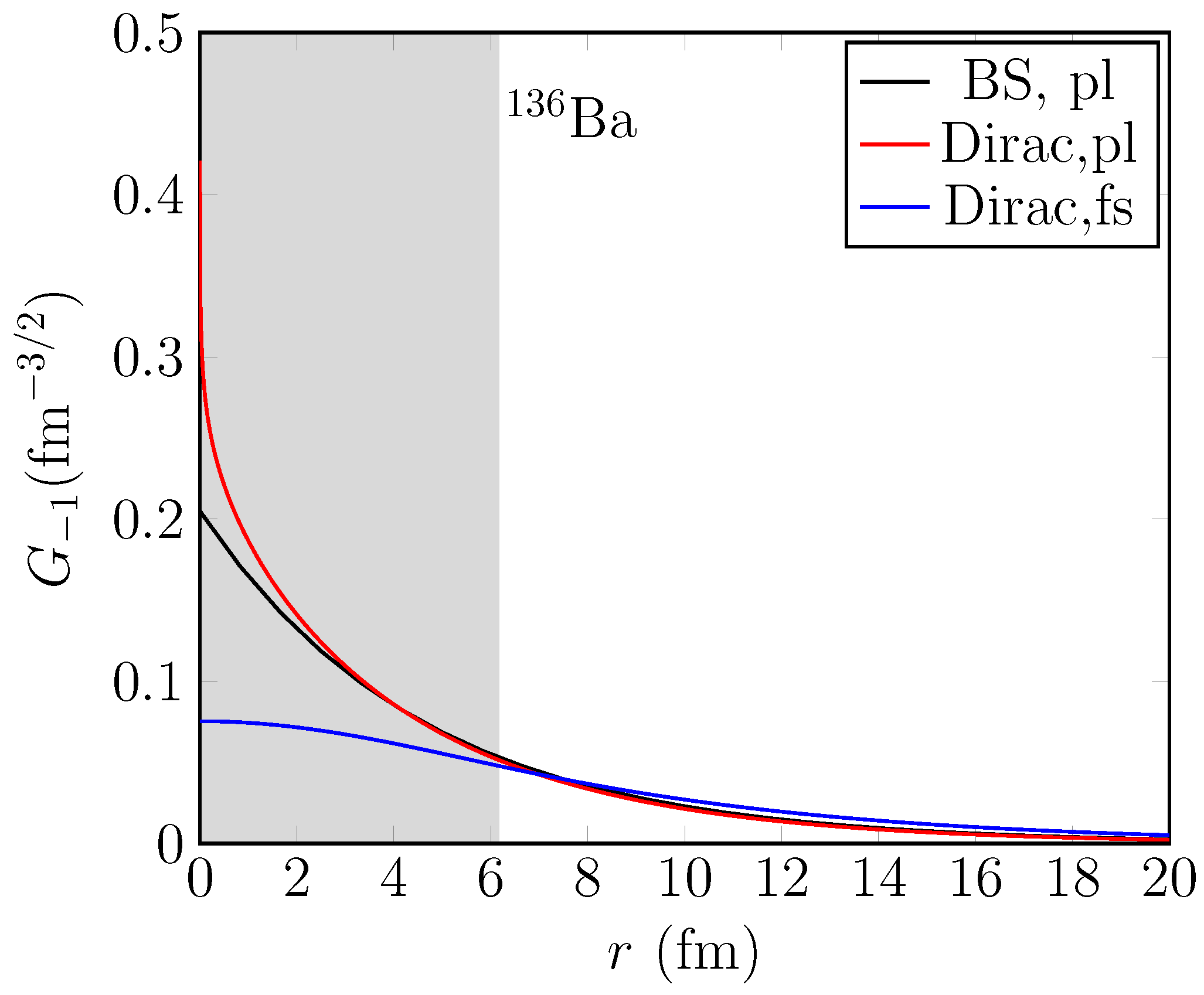
2.1. Bound-Muon S-Orbital Wave Function

Here we compute the OMC rates by using the formalism of Morita and Fujii [17]. In this formalism, it is straightforward to implement the exact Dirac wave function of the muon, as described in detail in Reference [18]. The Dirac wave function can be written as
ψ μ ( κ , μ ; r ) = ψ κ μ ( μ ) = i F κ ( r ) χ κ μ ( r ^ ) G κ ( r ) χ κ μ ( r ^ ) ,
where G κ and F κ are the radial wave functions of the bound state [17] and χ κ μ are normalized spherical spinors. The index κ is related to the orbital quantum number l in the following manner
l = κ and j = l 1 2 for κ > 0 l = κ 1 and j = l + 1 2 for κ < 0 .
After being stopped in the outer shells of an atom, the negative muon transits to the lowest atomic orbital, the 1 s 1 / 2 state, which corresponds to κ = 1 and μ = ± 1 / 2 . The corresponding large and small components of the bound-muon wave function— G 1 and F 1 —from Equation (2) can be numerically solved from the Dirac wave equations in the Coulomb field created by the nucleus [18]. Here we assume a nucleus with a uniform spherical charge distribution with a charge radius R c = r 0 A 1 / 3 and with r 0 = 1.2 fm and A being the nuclear mass number. The large component of the wave function accounts for a major part of the physics of the captured muon, while the small part accounts only for some 1% of the wave function, see, e.g., Figure 1 in Reference [18]. Hence, we can safely neglect the small part. The G 1 part can be compared with the Bethe–Salpeter (BS) equation [35] for a point nucleus:
G 1 = ( 2 Z / a 0 ) 3 2 1 + γ 2 Γ ( 2 γ + 1 ) 2 Z r a 0 γ 1 e Z r / a 0 .
Here, Z is the atomic number of the nucleus, γ = 1 ( α Z ) 2 , with the fine-structure constant α and the Bohr radius of the μ -mesonic atom
a 0 = 1 m μ α .
Here we have defined the reduced muon mass as
m μ = m μ 1 + m μ A M ,
where M is the (average) nucleon mass, and A M is the mass of the mother (and daughter) nucleus.
In Figure 1, we display the exact Dirac s-orbital wave function (large component) and its various degrees of approximation for 136 Ba. In the figure, it can be seen that the point–nucleus exact wave function and its BS approximation are quite close to each other, except at very short distances r 3 fm. Contrary to this, the exact finite-nucleus Dirac wave function deviates considerably from the other two, especially within the nucleus (the gray band in the figure). This is a much more drastic effect than the corresponding one for a light nucleus, such as 24 Mg (see Figure 1 of [18]).

2.2. Muon-Capture Rates

Calculation of the OMC rates is achieved using the Morita–Fujii formalism [17] and its extension developed in References [36,37] in order to treat small OMC rates in a more reliable way. The OMC rate of the process (1) can be expressed as
W = 2 P ( 2 J f + 1 ) 1 q m μ + A M q 2 ,
where the momentum exchange (q value) can be expressed as
q = ( m μ W 0 ) 1 m μ 2 ( m μ + A M ) .
Here, J f is the final-state spin-parity, M the average nucleon mass, and m μ ( m e ) is the rest mass of the muon (electron). The threshold energy W 0 = M f M i + m e + E X contains M i and M f as the masses of the initial and final nuclei and E X the excitation energy of the final nuclear state in 136 Cs. The rate function P contains the nuclear matrix elements, phase–space factors, and combinations of the weak couplings g A (axial–vector coupling), g P (induced pseudoscalar coupling), and g M = 1 + μ p μ n (induced weak-magnetism coupling), where μ p and μ n are the anomalous magnetic moments of the proton and the neutron. In the present work, we use the Goldberger–Treiman partially conserved axial vector current (PCAC) value for the ratio of the two axial-type couplings:
g P / g A = 2 M q q 2 + m π 2 6.8 ,
where m π = 138.04 MeV is the pion rest mass. Unless otherwise indicated, we adopt the free-neutron value g A = 1.27 in our calculations. Explicit expressions for the rate function P, containing all of the next-to-leading-order terms, can be found in detail in Reference [37], and we do not repeat those expressions in this article. It should be noted that at low excitation energies, as considered in the present work, W 0 / m μ 1 and, hence, the nuclear matrix elements in P depend only weakly on the excitation energy E X of the nuclear state.

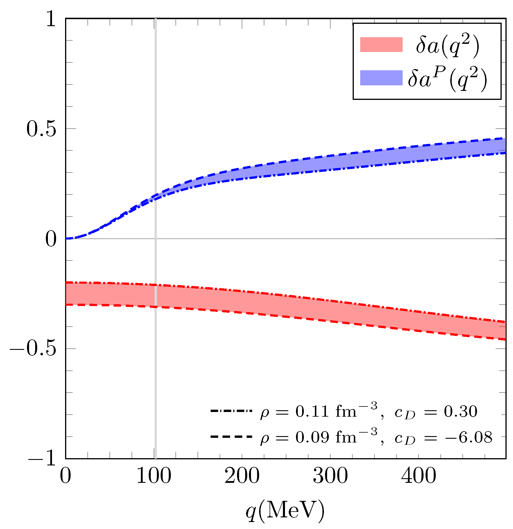
2.3. Chiral Two-Body Currents

We take the effect of the 2BC into account by making the replacements
g A ( 1 + δ a ( q 2 ) ) g A
and
g P 1 q 2 + m π 2 q 2 δ a P ( q 2 ) g P ,
where the 2BC contributions δ a ( q 2 ) and δ a P ( q 2 ) are approximated by the normal-ordered one-body part of the chiral two-body currents, as was achieved in Reference [38]. Normal ordering is conducted with respect to a Fermi gas reference state with density ρ . In the present work, we take the involved integrals in δ a ( q 2 ) and δ a P ( q 2 ) to be those of [39] with the density range ρ = 0.09–0.11 fm 3 . We use the same values of the involved constants as in Reference [38], as does Reference [40]. For the low-energy constants (LEC) c 1 , c 3 , c 4 , c 6 , and c D involved in the currents, we used the values listed in Table V of Reference [38]. The constant c D was adjusted in Reference [38] so that the axial vector correction δ a ( q 2 ) corresponded to the typical 20–30% axial vector quenching (or g A eff = 0.89–1.02 in terms of an effective coupling) at q = 0 MeV: the pair ( ρ = 0.09 fm 3 , c D = 6.08 ) giving the most quenching and ( ρ = 0.11 fm 3 , c D = 0.3 ) the least. We use the ranges of δ a ( q 2 ) and δ a P ( q 2 ) produced by these parameter choices for quantification of the uncertainties of our computed OMC rates. The corresponding 2BCs are displayed in Figure 2 where the relevant momentum exchange region is indicated by a vertical band. For the excitation energy region discussed in the present work, the momentum exchanges are contained within the interval q OMC = 101.5–102.6 MeV and the 2BC contributions within the intervals δ a ( q 2 ) = (0.210–0.310) and δ a P ( q 2 ) = 0.178–0.180.
The corrections coming from the inclusion of the 2BC at the relevant momentum exchange region correspond to a range g A eff ( q OMC ) = 0.88–1.00 of quenched values of the weak axial coupling and a range of g P eff ( q OMC ) = 4.26–4.27 of quenched values of the induced pseudoscalar coupling.

2.4. Many-Body Methods

In the present work, we used the interacting shell model (ISM) [41] and the proton–neutron quasiparticle random-phase approximation (pnQRPA) [42] to compute the ground state wave function of 136 Ba and the ground and excited states of 136 Cs. There have been several earlier ISM calculations of the DBD characteristics of the 136 Xe– 136 Cs– 136 Ba triplet of nuclei [6,7,8,9]. In these calculations, the jj55pn model space with the single-particle orbitals 2 s 1 / 2 , 1 d 3 / 2 , 1 d 5 / 2 , 0 g 7 / 2 , and 0 h 11 / 2 was adopted for both protons and neutrons. Here, we adopted the same model space and used the sn100pn [43] interaction, whose Hamiltonian consists of neutron–neutron ( n n ) , proton–neutron ( p n ) , and proton–proton ( p p ) interactions, with the latter containing the Coulomb interaction. The single-particle energies were −9.68, −8.72, −7.34, −7.24, and −6.88 MeV for the proton and −9.74, −8.97, −7.62, −7.31, and −7.38 MeV for the neutron 0 g 7 / 2 , 1 d 5 / 2 , 2 s 1 / 2 , 1 d 3 / 2 , and 0 h 11 / 2 orbitals, respectively [43]. In Reference [8], a quenching factor q = 0.45 was used for the spin–isospin operator σ τ , and in References [6,7,9], q = 0.74 was used. The latter quenching corresponds to a value g A eff = 0.93 of the effective value of the axial vector coupling. We adopted this value of g A eff in this work, as benchmarked by the three mentioned ISM calculations and preferred by the quenching through the 2BC, the associated g A eff interval discussed at the end of Section 2.3. In the actual ISM computations, we used the NuShellX@MSU code with its interaction libraries [44].
The pnQRPA correctly accounts for the gross features of spin–isospin strength functions, such as (p,n) and (n,p) reactions [4]. On the other hand, the pnQRPA typically poorly describes the fine structure of the low-lying states in odd–odd nuclei. In the present study, we wanted to test the capabilities of pnQRPA in producing the low-energy excitation spectrum in 136 Cs through the comparison of its results with those of the ISM. We used the same large, no-core, single-particle bases for protons and neutrons as in Reference [45]. These bases are based on Coulomb-corrected Woods–Saxon potential [46] and are slightly modified in the vicinity of the respective Fermi surfaces. All of the basic features of the pnQRPA are covered in detail in Reference [42]. It suffices to know that the pnQRPA is based on the BCS theory of superconductivity [47] and that the pairing strengths for the protons and neutrons were obtained through matching with the observed proton and neutron separation energies in the reference even–even nucleus [42], in this case 136 Ba. Furthermore, we used the method of Reference [48] to divide the renormalization of the effective two-body Bonn-A G-matrix interaction [49] into particle–hole and particle–particle parts by using the effective adjustable strength parameters g ph and g pp , known as the particle–hole and particle–particle strength parameters, respectively. The particle–hole parameter— g ph —is typically adjusted to the centroid energy of the Gamow–Teller giant resonance (GTGR) in the adjacent odd–odd nucleus of the even–even reference nucleus. Here, we resorted to the same method and adjusted it to the known GTGR energy in 136 Cs [45] in order to obtain the value g ph = 1.18 .
In Reference [45], a refined method concerning the g pp parameter was adopted: following the original idea put forth in Reference [50], a scheme called partial isospin restoration (PIR) was adopted. In the present work, we followed the PIR by multiplying the isoscalar ( T = 0 ) and isovector ( T = 1 ) parts of the particle–particle matrix elements of the G-matrix by the strength parameters g pp T = 0 and g pp T = 1 , respectively. The isovector strength was adjusted such that the Fermi part of the two-neutrino double-beta-decay (TNDBD) NME, corresponding to the transition 136 Xe 136 Ba , vanished, leading to a partial isospin restoration of the T = 1 proton–neutron, proton–proton, and neutron–neutron pairing channels. The isoscalar strength was subsequently varied so as to reproduce the measured half-life of the mentioned TNDBD transition [51].

3. Results and Discussion

First, we performed benchmark calculations in both the ISM and pnQRPA, omitting the 2BC contributions and using the free-nucleon value g A = 1.27 and the corresponding pseudoscalar coupling g P = 8.64 following from the Goldberger–Treiman relation (9). In the pnQRPA calculations, we adjusted the particle–particle parameters via the PIR scheme. We will use the shorthand notations sm-1BC and qrpa-1BC for these methods henceforth. Next, we performed more realistic calculations, taking into account the missing 2BC and the deficiencies of the many-body methods. We performed four different evaluations of the OMC rates, naming them as:
sm-2BC:
We performed an ISM calculation using the sn100pn interaction [43] by quenching the free axial vector couplings g A = 1.27 and g P = 8.64 using the 2BC according to Equations (10) and (11).
sm-phen:
We performed an ISM calculation like above, but this time, we used the phenomenologically obtained quenched value g A eff = 0.93 [9] and the value g P eff = 6.32 obtained through the Goldberger–Treiman relation (9).
qrpa-2BC:
We used the pnQRPA method as described in Section 2.4 and quenched g A and g P with the 2BC using Equations (10) and (11). We used the PIR scheme and adjusted the isoscalar strength to a value of g pp T = 1 = 0.86 in order to achieve the partial isospin restoration, then we adjust the isoscalar strength to the values g pp T = 0 = 0.65 ( g pp T = 0 = 0.67 ) in order to reproduce the TNDBD half-life t 1 / 2 ( 2 ν ) = ( 2.18 ± 0.05 ) · 10 21 yr [51] using the effective coupling g A eff = 0.89 ( g A eff = 1.02 ) corresponding to the free nucleon value g A = 1.27 quenched by the zero-momentum transfer correction δ a ( 0 ) through Equation (10) with parameters ρ = 0.09 fm 3 and c D = 6.08 ( ρ = 0.11 fm 3 and c D = 0.30 ) .
qrpa-phen:
Again, we used the pnQRPA method like above, but we used as the particle–particle strength the value g pp T = 0 = g pp T = 1 = 0.7 , which was obtained from the extensive survey of the β -decay and TNDBD half-lives within the mass range A = 100–136 in Reference [52]. We adopted the effective coupling g A eff = 0.83 resulting from the so-called linear g A model of the same work. This value is somewhat below the range of values g A eff = 0.89–1.02 corresponding to the axial vector correction δ a ( 0 ) at zero-momentum transfer. The corresponding effective pseudoscalar coupling is g P eff = 5.64 , as obtained through the Goldberger–Treiman relation (9). The value g A eff = 0.83 can be considered to account for both the missing two-body currents at q = 0 MeV and the deficiencies of the many-body approach in the spirit of Reference [16]. However, it does not take into account the momentum dependence of the two-body currents.
A summary of the values of all of the involved couplings and parameters is made in Table 1. We only considered the OMC rates of states with angular momenta J 5 , since the OMC rates of states with higher angular momenta are negligible.
We started by comparing the calculated ISM and pnQRPA excitation spectra of 136 Cs with the experimental ones, the results being shown in Figure 3. The pnQRPA calculations were conducted according to the schemes qrpa-2BC and qrpa-phen. It is worth noting that there are three sets of the pnQRPA-computed energies based on the three different values of the ( g pp T = 0 , g pp T = 1 ) pairs used in the pnQRPA calculations. Here, we plotted just one set of energies in the qrpa-2BC scheme, since the two sets of energy are almost identical. From Figure 3, it can be seen that the densities of both the ISM- and pnQRPA-computed states are quite similar, higher than the densities of the measured states. It is, in fact, remarkable that both theories predict low-energy spectra so similarly, with pnQRPA able to reproduce the density of the ISM states. The density of the experimental spectrum is smaller than predicted by the computations, probably due to difficulties in observing some of the states.
The results of the OMC calculations are presented in Table 2 (ISM results) and Table 3 (pnQRPA results). In Table 2, the first column displays the spin parity of the final state and the second column its excitation energy in MeV (in order of increasing energy). The third to fifth columns give the ISM-computed OMC rates in units of 10 3 1/s. The third column (1BC) corresponds to an ISM calculation without the 2BC contribution, and the fourth column corresponds to the same calculation with the 2BC contribution included (the sm-2BC calculational scheme). The fifth column lists the OMC rates obtained by using the phenomenological sm-phen calculational scheme. Table 3 has a similar structure, but now there are two sets of qrpa-2BC energies (column 2) corresponding to the two sets of LEC used in our calculations and the set of qrpa-phen energies in column 3. Columns 4–6 list the OMC rates obtained by using the schemes qrpa-1BC, qrpa-2BC, and qrpa-phen.
The first observation from columns three and four of Table 2 and Table 3 is that the two-body currents, included either via the 2BC corrections δ a ( q 2 ) and δ a P ( q 2 ) or phenomenologically via effective couplings, affect the OMC rates considerably, on average by some (30–40)%, but up to almost 50% in some cases.
The total rates of these states are summarized in Table 4, indicating that in both models, the most important contributions come from the 1 + , 2 + , 2 , and 3 + states. The pnQRPA states are able to catch more collectivity of the 1 + and 2 + states, particularly for the 1 1 + state, which is quite collective in the pnQRPA.
In order to relate the pnQRPA results to previous measurements, one can take a look at the computations in Reference [37]. There, the rates of the OMC of several double-beta daughter nuclei, particularly of 136 Ba, were computed by using large, no-core, single-particle spaces and the effective Bonn-A potential, quite like in the present work. In those calculations, the effective values g A eff = 0.80 and g P eff = 7.0 were adopted, which are values close to those of our qrpa-phen scheme and not far from our qrpa-2BC calculational scheme. This makes the three computations very comparable, particularly for the OMC of 136 Ba, but also for 76 Se, where experimental data exist. In Table V of Reference [37], the pnQRPA-computed OMC rates of final states in 76 As, below some 1 MeV of excitation like in the present work, were compared with the corresponding experimental ones, and a surprisingly good correspondence was found. There, the total rate for the OMC of the 0 + , 1 + , 1 , 2 + , 2 , 3 + , 3 , 4 + , and 4 final states in 76 As was 665 × 10 3 1/s in the experiment and 675 × 10 3 1/s in the pnQRPA. These total OMC rates are in line with the total OMC rates of (674–807) × 10 3 1/s and 592 × 10 3 1/s of our qrpa-2BC and qrpa-phen calculational schemes, respectively. Notably, both in the experiment and in the pnQRPA calculation of Reference [37], the 1 + rate was the largest one with the values 218 × 10 3 1/s for the experiment and 237 × 10 3 1/s for the pnQRPA, comparable with our (243–303) × 10 3 1/s and 207 × 10 3 1/s in the qrpa-2BC and qrpa-phen calculational schemes. In Reference [37] also, the OMC of 2 states was strong, some 10 times stronger than in the present calculations, since the role of 2 states in p f -shell nuclei is quite pronounced [4].
The measured total rate in 136 Ba, including all of the possible final states, features 11,100 × 10 3 1/s [55]. This means that the OMC rate of states below 1 MeV accounts for some 1.5% of the total rate for the sm-2BC scheme, 1.4% of the total rate for the sm-phen scheme, 6–7% of the total rate for the qrpa-2BC scheme, and 5.3% of the total rate for the qrpa-phen scheme, thus being below 10% but still non-negligible. This highlights the importance of comparison with the potential future experimental data and the emerging implications for the virtual NDBD transitions below roughly 1 MeV of excitation in the intermediate nucleus of a double-beta triplet of nuclei.
In the end, it would be highly interesting to compare the presently computed OMC rates to individual final states and the total OMC rate below 1 MeV with future experimental results by the MONUMENT Collaboration [56]. This will open up the possibility to probe the nuclear wave functions within the considered 1 MeV excitation energy interval in 136 Cs. At the same time, we can gain information on the value of both g A and g P , the weak axial coupling and the induced pseudoscalar coupling, in a momentum-exchange range relevant for the NDBD [22]. This gained information helps improve the precision of the nuclear matrix elements of the NDBD and thus reflects on the sensibility estimates of presently-running and future NDBD experiments.

4. Conclusions

In the present work, we computed the rates of ordinary muon capture on 136 Ba to low-lying nuclear states (below roughly 1 MeV of excitation energy) in 136 Cs, 136 Ba being the daughter nucleus of 136 Xe double-beta decay. The capture rates were computed by using the interacting shell model (ISM) and proton–neutron quasiparticle random-phase approximation (pnQRPA). Furthermore, the chiral two-body meson-exchange currents and the exact s-orbital Dirac wave function of the captured muon were used in the numerical computations. The computed energy spectra and the capture rates below 1 MeV of excitation in 136 Cs were surprisingly similar for both the ISM and the pnQRPA, the experimental low-energy spectrum being less dense. The chiral two-body currents reduce the capture rates by some (30–40)% on average, and the summed capture rates below 1 MeV of excitation in 136 Cs account for some (1–7)% of the total measured capture rate, thus being potentially a sizable portion of the total capture rate. Comparison of the capture rates with future experimental data opens up possibilities for accessing the wave functions of low-energy states in 136 Cs and the effective values of the weak axial-type couplings, relevant for the neutrinoless double-beta decay of 136 Xe and beyond.

Author Contributions

Ordinary muon capture rates and pnQRPA calculations, P.G.; parameter values and supervision of the computations, L.J.; calculation of the relativistic muon wave function, J.K.; nuclear shell-model calculations, M.R.; original idea of the project, coordination and supervision of the computations, and writing of the first draft of the paper, J.S. All authors have read and agreed to the published version of the manuscript.

Funding

This research was funded by the Academy of Finland, grants No. 314733, No. 320062, and No. 345869 and by the Arthur B. McDonald Canadian Astroparticle Physics Research Institute. TRIUMF received federal funding via a contribution agreement with the National Research Council of Canada.

Data Availability Statement

Not applicable.

Conflicts of Interest

The authors declare no conflict of interest.

Note

1
In the present work, we use the convention c = 1 for compactness of presentation.

References

  1. Suhonen, J.; Civitarese, O. Weak-interaction and nuclear-structure aspects of nuclear double beta decay. Phys. Rep. 1998, 300, 123–214. [Google Scholar] [CrossRef]
  2. Vergados, J.D.; Ejiri, H.; Šimkovic, F. Neutrinoless double beta decay and neutrino mass. Int. J. Mod. Phys. E 2016, 25, 1630007. [Google Scholar] [CrossRef] [Green Version]
  3. Engel, J.; Menéndez, J. Status and future of nuclear matrix elements for neutrinoless double-beta decay: A review. Rep. Prog. Phys. 2017, 80, 046301. [Google Scholar] [CrossRef] [PubMed] [Green Version]
  4. Ejiri, H.; Suhonen, J.; Zuber, K. Neutrino-nuclear responses for astro-neutrinos, single beta decays and double beta decays. Phys. Rep. 2019, 797, 1–102. [Google Scholar] [CrossRef]
  5. Agostini, M.; Benato, G.; Detwiler, J.A.; Menéndez, J.; Vissani, F. Toward the discovery of matter creation with neutrinoless double-beta decay. arXiv 2022, arXiv:2202.01787. [Google Scholar]
  6. Caurier, E.; Nowacki, F.; Poves, A.; Retamosa, J. Shell Model Studies of the Double Beta Decays of 76Ge, 82Se, and 136Xe. Phys. Rev. Lett. 1996, 77, 1954–1957. [Google Scholar] [CrossRef] [Green Version]
  7. Caurier, E.; Menéndez, J.; Nowacki, F.; Poves, A. Influence of Pairing on the Nuclear Matrix Elements of the Neutrinoless ββ Decays. Phys. Rev. Lett. 2008, 100, 052503. [Google Scholar] [CrossRef] [Green Version]
  8. Caurier, E.; Nowacki, F.; Poves, A. Shell Model description of the ββ decay of 136Xe. Phys. Lett. B 2012, 711, 62–64. [Google Scholar] [CrossRef] [Green Version]
  9. Horoi, M.; Brown, B.A. Shell-Model Analysis of the 136Xe Double Beta Decay Nuclear Matrix Elements. Phys. Rev. Lett. 2013, 110, 222502. [Google Scholar] [CrossRef] [Green Version]
  10. Suhonen, J.; Civitarese, O. Double-beta-decay nuclear matrix elements in the QRPA framework. J. Phys. G Nucl. Part. Phys. 2012, 39, 085105. [Google Scholar] [CrossRef]
  11. Märkisch, B.; Mest, H.; Saul, H.; Wang, X.; Abele, H.; Dubbers, D.; Klopf, M.; Petoukhov, A.; Roick, C.; Soldner, T.; et al. Measurement of the Weak Axial-Vector Coupling Constant in the Decay of Free Neutrons Using a Pulsed Cold Neutron Beam. Phys. Rev. Lett. 2019, 122, 242501. [Google Scholar] [CrossRef] [Green Version]
  12. Suhonen, J.T. Value of the Axial-Vector Coupling Strength in β and ββ Decays: A Review. Front. Phys. 2017, 5, 55. [Google Scholar] [CrossRef] [Green Version]
  13. Ejiri, H. Axial-vector weak coupling at medium momentum for astro neutrinos and double beta decays. J. Phys. G Nucl. Part. Phys. 2019, 46, 125202. [Google Scholar] [CrossRef] [Green Version]
  14. Ejiri, H. Nuclear Matrix Elements for β and ββ Decays and Quenching of the Weak Coupling gA in QRPA. Front. Phys. 2019, 7, 30. [Google Scholar] [CrossRef]
  15. Menéndez, J.; Gazit, D.; Schwenk, A. Chiral Two-Body Currents in Nuclei: Gamow-Teller Transitions and Neutrinoless Double-Beta Decay. Phys. Rev. Lett. 2011, 107, 062501. [Google Scholar] [CrossRef] [PubMed] [Green Version]
  16. Gysbers, P.; Hagen, G.; Holt, J.; Jansen, G.; Morris, T.; Navrátil, P.; Papenbrock, T.; Quaglioni, S.; Schwenk, A.; Stroberg, S.; et al. Discrepancy between experimental and theoretical β-decay rates resolved from first principles. Nat. Phys. 2019, 15, 1. [Google Scholar] [CrossRef] [Green Version]
  17. Morita, M.; Fujii, A. Theory of Allowed and Forbidden Transitions in Muon Capture Reactions. Phys. Rev. 1960, 118, 606–618. [Google Scholar] [CrossRef]
  18. Jokiniemi, L.; Miyagi, T.; Stroberg, S.R.; Holt, J.D.; Kotila, J.; Suhonen, J. Ab initio calculation of muon capture on 24Mg. Phys. Rev. C 2023, 107, 014327. [Google Scholar] [CrossRef]
  19. Measday, D. The nuclear physics of muon capture. Phys. Rep. 2001, 354, 243–409. [Google Scholar] [CrossRef]
  20. Kortelainen, M.; Suhonen, J. Ordinary muon capture as a probe of virtual transitions of ββ decay. Europhys. Lett. 2002, 58, 666. [Google Scholar] [CrossRef] [Green Version]
  21. Kortelainen, M.; Suhonen, J. Nuclear muon capture as a powerful probe of double-beta decays in light nuclei. J. Phys. G Nucl. Part. Phys. 2004, 30, 2003. [Google Scholar] [CrossRef]
  22. Siiskonen, T.; Hjorth-Jensen, M.; Suhonen, J. Renormalization of the weak hadronic current in the nuclear medium. Phys. Rev. C 2001, 63, 055501. [Google Scholar] [CrossRef] [Green Version]
  23. Jokiniemi, L.; Suhonen, J. Comparative analysis of muon-capture and 0νββ-decay matrix elements. Phys. Rev. C 2020, 102, 024303. [Google Scholar] [CrossRef]
  24. Asakura, K.; Gando, A.; Gando, Y.; Hachiya, T.; Hayashida, S.; Ikeda, H.; Inoue, K.; Ishidoshiro, K.; Ishikawa, T.; Ishio, S.; et al. Search for double-beta decay of 136Xe to excited states of 136Ba with the KamLAND-Zen experiment. Nucl. Phys. A 2016, 946, 171–181. [Google Scholar] [CrossRef] [Green Version]
  25. Albert, J.B.; Anton, G.; Badhrees, I.; Barbeau, P.S.; Bayerlein, R.; Beck, D.; Belov, V.; Breidenbach, M.; Brunner, T.; Cao, G.F.; et al. Search for Neutrinoless Double-Beta Decay with the Upgraded EXO-200 Detector. Phys. Rev. Lett. 2018, 120, 072701. [Google Scholar] [CrossRef] [Green Version]
  26. Shimizu, I.; Chen, M. Double Beta Decay Experiments with Loaded Liquid Scintillator. Front. Phys. 2019, 7, 33. [Google Scholar] [CrossRef] [Green Version]
  27. Kharusi, S.; Anton, G.; Badhrees, I.; Barbeau, P.; Beck, D.; Belov, V.; Bhatta, T.; Breidenbach, M.; Brunner, T.; Cao, G.; et al. Search for Majoron-emitting modes of Xe 136 double beta decay with the complete EXO-200 dataset. Phys. Rev. D 2021, 104, 112002. [Google Scholar] [CrossRef]
  28. The MONUMENT Collaboration, See the Contribution List of the MEDEX’22 Workshop, Prague, Czech Republic. 13–17 June 2022. Available online: https://indico.utef.cvut.cz/event/32/contributions (accessed on 3 June 2023).
  29. Measday, D.F.; Stocki, T.J.; Ricardo, A.; Cole, P.L.; Chaden, D.; Fernando, U. Comparison of Muon Capture in Light and in Heavy Nuclei. AIP Conf. Proc. 2007, 947, 253. [Google Scholar] [CrossRef]
  30. Measday, D.F.; Stocki, T.J.; Tam, H. Gamma rays from muon capture in I, Au, and Bi. Phys. Rev. C 2007, 75, 045501. [Google Scholar] [CrossRef]
  31. Hashim, I.H.; Ejiri, H.; Shima, T.; Takahisa, K.; Sato, A.; Kuno, Y.; Ninomiya, K.; Kawamura, N.; Miyake, Y. Muon capture reaction on 100Mo to study the nuclear response for double-β decay and neutrinos of astrophysics origin. Phys. Rev. C 2018, 97, 014617. [Google Scholar] [CrossRef] [Green Version]
  32. Hashim, I.H.; Ejiri, H. New Research Project with Muon Beams for Neutrino Nuclear Responses and Nuclear Isotopes Production. AAPPS Bull. 2019, 29, 21–26. [Google Scholar] [CrossRef]
  33. Hashim, I.; Ejiri, H.; Othman, F.; Ibrahim, F.; Soberi, F.; Ghani, N.; Shima, T.; Sato, A.; Ninomiya, K. Nuclear isotope production by ordinary muon capture reaction. Nucl. Instrum. Methods Phys. Res. Sect. A Accel. Spectrometers Detect. Assoc. Equip. 2020, 963, 163749. [Google Scholar] [CrossRef] [Green Version]
  34. Hashim, I.H.; Ejiri, H. Ordinary Muon Capture for Double Beta Decay and Anti-Neutrino Nuclear Responses. Front. Astron. Space Sci. 2021, 8, 666383. [Google Scholar] [CrossRef]
  35. Bethe, H.; Salpeter, E. Quantum Mechanics of One- and Two-Electron Atoms; Academic Press: New York, NY, USA, 1959. [Google Scholar]
  36. Jokiniemi, L.; Suhonen, J.; Ejiri, H.; Hashim, I. Pinning down the strength function for ordinary muon capture on 100Mo. Phys. Lett. B 2019, 794, 143–147. [Google Scholar] [CrossRef]
  37. Jokiniemi, L.; Suhonen, J. Muon-capture strength functions in intermediate nuclei of 0νββ decays. Phys. Rev. C 2019, 100, 014619. [Google Scholar] [CrossRef] [Green Version]
  38. Hoferichter, M.; Menéndez, J.; Schwenk, A. Coherent elastic neutrino-nucleus scattering: EFT analysis and nuclear responses. Phys. Rev. D 2020, 102, 074018. [Google Scholar] [CrossRef]
  39. Klos, P.; Menéndez, J.; Gazit, D.; Schwenk, A. Large-scale nuclear structure calculations for spin-dependent WIMP scattering with chiral effective field theory currents. Phys. Rev. D 2013, 88, 083516. [Google Scholar] [CrossRef] [Green Version]
  40. Jokiniemi, L.; Romeo, B.; Soriano, P.; Menéndez, J. Neutrinoless ββ-decay nuclear matrix elements from two-neutrino ββ-decay data. Phys. Rev. C 2022, 107, 044305. [Google Scholar] [CrossRef]
  41. Caurier, E.; Martínez-Pinedo, G.; Nowacki, F.; Poves, A.; Zuker, A.P. The shell model as a unified view of nuclear structure. Rev. Mod. Phys. 2005, 77, 427–488. [Google Scholar] [CrossRef] [Green Version]
  42. Suhonen, J. From Nucleons to Nucleus: Concepts of Microscopic Nuclear Theory; Theoretical and Mathematical Physics; Springer: Berlin/Heidelberg, Germany, 2007. [Google Scholar] [CrossRef] [Green Version]
  43. Brown, B.A.; Stone, N.J.; Stone, J.R.; Towner, I.S.; Hjorth-Jensen, M. Magnetic moments of the 2 1 + states around 132Sn. Phys. Rev. C 2005, 71, 044317. [Google Scholar] [CrossRef] [Green Version]
  44. Brown, B.; Rae, W. The Shell-Model Code NuShellX@MSU. Nucl. Data Sheets 2014, 120, 115–118. [Google Scholar] [CrossRef]
  45. Jokiniemi, L.; Ejiri, H.; Frekers, D.; Suhonen, J. Neutrinoless ββ nuclear matrix elements using isovector spin-dipole Jπ = 2 data. Phys. Rev. C 2018, 98, 024608. [Google Scholar] [CrossRef] [Green Version]
  46. Bohr, A.; Mottelson, B.R. Nuclear Structure; Benjamin: New York, NY, USA, 1969; Volume I. [Google Scholar]
  47. Bardeen, J.; Cooper, L.N.; Schrieffer, J.R. Microscopic Theory of Superconductivity. Phys. Rev. 1957, 106, 162–164. [Google Scholar] [CrossRef] [Green Version]
  48. Suhonen, J.; Taigel, T.; Faessler, A. pnQRPA calculation of the β+/EC quenching for several neutron-deficient nuclei in mass regions A = 94–110 and A = 146–156. Nucl. Phys. A 1988, 486, 91–117. [Google Scholar] [CrossRef]
  49. Holinde, K. Two-nucleon forces and nuclear matter. Phys. Rep. 1981, 68, 121–188. [Google Scholar] [CrossRef]
  50. Šimkovic, F.; Rodin, V.; Faessler, A.; Vogel, P. 0νββ and 2νββ nuclear matrix elements, quasiparticle random-phase approximation, and isospin symmetry restoration. Phys. Rev. C 2013, 87, 045501. [Google Scholar] [CrossRef] [Green Version]
  51. Barabash, A. Precise Half-Life Values for Two-Neutrino Double-β Decay: 2020 review. Universe 2020, 6, 159. [Google Scholar] [CrossRef]
  52. Pirinen, P.; Suhonen, J. Systematic approach to β and 2νββ decays of mass A=100–136 nuclei. Phys. Rev. C 2015, 91, 054309. [Google Scholar] [CrossRef] [Green Version]
  53. ENSDF Database. Available online: http://www.nndc.bnl.gov/ensdf/ (accessed on 3 June 2023).
  54. Rebeiro, B.M.; Triambak, S.; Garrett, P.E.; Ball, G.C.; Brown, B.A.; Menéndez, J.; Romeo, B.; Adsley, P.; Lenardo, B.G.; Lindsay, R.; et al. 138Ba(d,α) Study of States in 136Cs: Implications for New Physics Searches with Xenon Detectors. arXiv 2023, arXiv:2301.11371. [Google Scholar]
  55. Suzuki, T.; Measday, D.F.; Roalsvig, J.P. Total nuclear capture rates for negative muons. Phys. Rev. C 1987, 35, 2212–2224. [Google Scholar] [CrossRef]
  56. The MONUMENT Collaboration. Work in progress.
Figure 1. Comparison of the large component of the exact muon wave function for a finite nucleus with a uniform spherical charge distribution (blue line) with a corresponding one for a point-like nucleus (red line) and its Bethe–Salpeter (BS) approximation (black line). The gray band denotes the range inside the nucleus.
Universe 09 00270 g001
Figure 2. The two-body currents used in the present work are functions of momentum exchange. The dashed lines denote the currents obtained by ρ = 0.09 fm 3 and c D = 6.08 , and the dotted lines indicate those obtained with ρ = 0.11 fm 3 and c D = 0.30 . The typical momentum exchange region of the transitions considered in the present work is denoted by a vertical gray band.
Universe 09 00270 g002
Figure 3. Excitation energy spectrum of 136 Cs. A comparison between the experimental spectrum and those computed by using the ISM and pnQRPA is shown here. The first experimental spectrum was taken from the ENSDF database [53], and the second one was taken from Rebeiro et al. in Reference [54]. Only states with angular momenta J 5 were considered.
Universe 09 00270 g003
Table 1. Values of the weak axial couplings, the Fermi gas density ρ , and the LEC c D and pnQRPA parameters used in our calculations.
sm-1BC and sm-2BCsm-phenqrpa-1BCqrpa-2BCqrpa-phen
g PP T = 0 --0.690.650.670.7
g PP T = 1 --0.860.860.860.7
g ph --1.181.181.181.18
g A 1.270.931.271.271.270.83
g P / g A 6.86.86.86.86.86.8
ρ 0.090.11--0.090.11-
c D −6.080.30--−6.080.30-
Table 2. ISM-computed energies (second column) and OMC rates (third to fifth columns) of the final states (f) of spin J and parity π (first column) with angular momenta J 5 . The bottom line summarizes the total OMC rates below some 1 MeV as summed over the OMC rates listed in columns three to five. The lower (upper) limits in column four correspond to the Fermi gas density ρ = 0.09 fm 3 and the low-energy constant c D = 6.08 ( ρ = 0.11 fm 3 and c D = 0.3 ), the rest of the LEC being equal in the two sets.
OMC Rate ( 10 3 1 / s)
J f π E(MeV)sm-1BCsm-2BCsm-phen
5 1 + 0.0000.06470.0661 (0.0836)0.0433
3 1 + 0.0234.022.75 (3.36)2.60
4 1 + 0.0391.501.36 (1.40)1.37
2 1 + 0.08310.65.62 (6.99)6.18
3 2 + 0.18112.06.24 (8.08)6.66
2 2 + 0.22520.112.8 (15.00)13.7
3 3 + 0.2444.942.48 (3.23)2.71
4 2 + 0.3235.833.50 (4.17)3.78
4 3 + 0.4986.004.34 (4.83)4.54
3 4 + 0.51731.216.8 (21.5)17.9
5 1 0.5220.6450.371 (0.451)0.404
3 1 0.54516.18.85 (11.0)9.73
1 1 + 0.5459.014.67 (6.03)5.03
4 1 0.54724.013.0 (16.7)13.7
2 3 + 0.61518.212.5 (14.2)13.2
5 2 0.6710.2510.190 (0.208)0.198
1 2 + 0.7520.2850.123 (0.163)0.146
4 2 0.7602.221.31 (1.65)1.32
2 4 + 0.8032.491.74 (1.95)1.83
4 4 + 0.8850.1430.0865 (0.103)0.0933
2 1 1.01678.641.5 (53.3)44.4
Sum ( 10 3 1 / s) 248140 (174)150
Table 3. pnQRPA-computed energies for the qrpa-2BC scheme (second column) and the qrpa-phen scheme (third column) and OMC rates (fourth to sixth columns) of the final states (f) of spin J and parity π (first column) with angular momenta J 5 . The bottom line summarizes the total OMC rates below 1 MeV as summed over the OMC rates listed in columns four to six. The two energies in column two and the lower (upper) limits in column five correspond to the Fermi gas density ρ = 0.09 fm 3 and the low-energy constant c D = 6.08 ( ρ = 0.11 fm 3 and c D = 0.3 ), the rest of the LEC being equal in the two sets.
OMC Rate ( 10 3 1 / s)
J f π E(MeV)qrpa-2BCE(MeV)qrpa-phenqrpa-1BCqrpa-2BCqrpa-phen
5 1 + 0.000 0.000 0.902 0.491 ( 0.601 ) 0.483
3 1 + 0.110 ( 0.107 ) 0.102 3.04 1.74 ( 2.19 ) 1.51
2 1 + 0.124 ( 0.122 ) 0.120 133 102 ( 111 ) 93.3
4 1 + 0.139 ( 0.144 ) 0.154 10.0 8.81 ( 9.34 ) 8.96
1 1 + 0.227 ( 0.213 ) 0.193 443 243.0 ( 303.4 ) 206.9
4 2 + 0.180 ( 0.179 ) 0.203 12.4 8.76 ( 9.61 ) 8.25
3 2 + 0.249 ( 0.254 ) 0.264 11.6 7.93 ( 10.8 ) 3.49
3 3 + 0.268 ( 0.273 ) 0.281 156 85.6 ( 108 ) 77.5
3 4 + 0.330 ( 0.332 ) 0.338 12.2 9.50 ( 11.9 ) 5.34
2 2 + 0.340 ( 0.346 ) 0.367 88.3 49.0 ( 60.2 ) 50.1
3 1 0.461 ( 0.459 ) 0.458 48.0 28.9 ( 34.4 ) 25.8
4 3 + 0.471 ( 0.477 ) 0.494 4.19 3.24 ( 3.60 ) 3.18
5 1 0.505 ( 0.509 ) 0.515 1.20 0.825 ( 0.933 ) 0.775
4 1 0.553 ( 0.555 ) 0.558 1.60 1.04 ( 1.19 ) 0.596
2 3 + 0.533 ( 0.538 ) 0.561 87.1 60.0 ( 68.3 ) 57.7
5 2 0.621 ( 0.624 ) 0.637 0.017 0.0135 ( 0.0149 ) 0.0178
4 2 0.681 ( 0.686 ) 0.695 43.1 24.1 ( 30.6 ) 20.5
2 1 0.750 ( 0.725 ) 0.704 27.3 26.6 ( 26.0 ) 14.2
3 2 0.896 ( 0.901 ) 0.926 20.5 12.7 ( 15.1 ) 12.9
Sum ( 10 3 1 / s) 1103 674 ( 807 ) 592
Table 4. Total OMC rates of each multipole J π as summed over the rates listed in Table 2 for the sm-2BC and sm-phen schemes and in Table 3 for the qrpa-2BC and qrpa-phen schemes. The lower (upper) limits in the second and fourth columns correspond to the Fermi gas density ρ = 0.09 fm 3 and the low-energy constant c D = 6.08 ( ρ = 0.11 fm 3 and c D = 0.3 ).
OMC Rate ( 10 3 1 / s)
J π sm-2BCsm-phenqrpa-2BCqrpa-phen
5 + 0.1 (0.1)0.00.5 (0.6)0.5
4 + 9.3 (10.5)9.820.8 (22.6)20.4
3 + 28.3 (36.2)29.9104.8 (132.9)87.8
2 + 32.7 (38.1)34.9211.0 (239.5)201.1
1 + 4.8 (6.2)5.2243.0 (303.4)206.9
5 0.6 (0.7)0.60.8 (0.9)0.8
4 14.3 (18.4)15.025.1 (31.8)21.2
3 8.9 (11.0)9.741.6 (49.5)38.7
2 41.5 (53.3)44.426.6 (26.0)14.2
Disclaimer/Publisher’s Note: The statements, opinions and data contained in all publications are solely those of the individual author(s) and contributor(s) and not of MDPI and/or the editor(s). MDPI and/or the editor(s) disclaim responsibility for any injury to people or property resulting from any ideas, methods, instructions or products referred to in the content.

