Article

Even and Odd Self-Similar Solutions of the Diffusion Equation for Infinite Horizon

by
László Mátyás
1,* and
Imre Ferenc Barna
2
1
Department of Bioengineering, Faculty of Economics, Socio-Human Sciences and Engineering, Sapientia Hungarian University of Transylvania, Libertătii sq. 1, 530104 Miercurea Ciuc, Romania
2
Wigner Research Center for Physics, Konkoly-Thege Miklós út 29-33, 1121 Budapest, Hungary
*
Author to whom correspondence should be addressed.
Universe 2023, 9(6), 264; https://doi.org/10.3390/universe9060264
Submission received: 23 February 2023 / Revised: 25 May 2023 / Accepted: 26 May 2023 / Published: 31 May 2023
(This article belongs to the Special Issue Zimányi School – Heavy Ion Physics)

Abstract

:
In the description of transport phenomena, diffusion represents an important aspect. In certain cases, the diffusion may appear together with convection. In this paper, we study the diffusion equation with the self-similar Ansatz. With an appropriate change of variables, we have found an original new type of solution of the diffusion equation for infinite horizon. We derive novel even solutions of diffusion equation for the boundary conditions presented. For completeness, the odd solutions are also mentioned as well, as part of the previous works. We have found a countable set of even and odd solutions, of which linear combinations also fulfill the diffusion equation. Finally, the diffusion equation with a constant source term is discussed, which also has even and odd solutions.

1. Introduction

It is evident that mass diffusion or heat conduction is a fundamental physical process which attracted enormous intellectual interest from mathematicians, physicists and engineers over the last two centuries. The existing literature about mass and heat diffusion is immense; we only mention some fundamental textbooks [1,2,3,4,5].
Regular diffusion is the cornerstone of many scientific disciplines, such as surface growth [6,7,8], reactions diffusion [9] or even flow problems in porous media. In our last two papers, we gave an exhaustive summary of such processes with numerous relevant reviews [10,11].
In connection with thermal diffusion [12,13], the simultaneous presence of heat and mass transfer is also possible, which may lead to cross effects [14]. One may find relevant applications related to general issues of heat transfer or engineering in [15]. Important diffusive phenomena occur in the universe [16], which is another field of interest.
The study of population dynamics or biological processes [17,18,19] also involves diffusive processes, especially in spatial extended systems. In environmental sciences, the effects of spreading, distribution and adsorption of particulate matter or pollutants are also relevant [20,21,22,23]. Furthermore, diffusion coefficients have been measured for practical purposes in food sciences as well [24].
New applications of diffusion have gained ground in social sciences in the last decades as well. As examples, we can mention diffusion of innovations [25,26], diffusion of technologies and social behavior [27] or even diffusion of cultures, humans or ideas [28,29]. One may also find aspects related to diffusion in the theory of pricing [30,31]. The structure of the network has also a crucial role which influences the spread of innovations, ideas or even computer viruses [32]. Parallel to such diffusion activities, generalization of heat-transport equations was done by Ván and coauthors [33], e.g., fourth-order partial differential equations (PDE)s were formulated to elaborate the problem of non-regular heat conduction phenomena. Finally, we should not forget the continuously developing numerical methods of PDEs; it is worth mentioning the new results obtained by Kovács and coworkers [34,35]. Such spirit of the times clearly shows that investigation of diffusion (and heat conduction) is still an important task.
Having in mind that diffusion can be a general, three-dimensional process beyond Cartesian symmetry, here we investigate the one-dimensional diffusion equation. The change in time of variable C ( x , t ) is influenced by the presence of it in the neighbors:
C ( x , t ) t = D 2 C ( x , t ) x 2 ,
where D is the diffusion coefficient which should have positive real values. Usually, it can be considered constant for given temperature and pressure in gases. A counter-example is the heat diffusion process in large-temperature-gradient semiconductor crystals where heat conduction coefficients have a complicated temperature dependence [36].
One assumes that C ( x , t ) is a sufficiently smooth function together with existing derivatives regarding both variables. In this general form, one may observe that if C ( x , t ) is a solution, then C ( x , t ) + C 0 is also a solution, where C 0 is a constant.
In this study, we consider a constant diffusion coefficient. From a practical point of view, a typical case is the diffusion in gases, where at constant temperature and constant pressure, the diffusion coefficient is constant as is described in [37].
For a finite horizon or interval, in case the concentration is fixed at the two ends C ( x = 0 , t ) = C 0 and C ( x = L , t ) = C 0 , the solutions are
C k ( x , t ) = C 0 + e D π 2 k 2 t L 2 · sin k π L x ,
where k = 1 , 2 , 3 ; it can be any positive integer number. In general, beyond C 0 , any linear combination of the product of the exponent and sine for different k is a solution. For finite horizon, in the case when the density is fixed to zero on both ends, the solutions are changed to
C k ( x , t ) = C 0 + e D π 2 n 2 t L 2 · cos n π L x ,
where n = 1 , 2 , 3 can be any positive integer number. Thanks to the Fourier theorem, with the help of Equations (2) and (3) arbitrary diffusion profile can be approximated on a closed interval. These are well-known analytic results and can be found in any usual physics textbooks such as [1,2].
In the present study—with the help of the self-similar Ansatz—we are going to present generic symmetric solutions for infinite horizon. These solutions have their roots at the very beginning of the theory, in the form of the Gaussian [1,2]:
C ( x , t ) = Const . · 1 t e x 2 4 D t .
For infinite horizon, there are also certain works which present a given aspect of the diffusion, and it may arrive to a slightly more general aspect than the classical solution presented above [38].
In the following, we will go much beyond that point and will present and analyze completely new type of solutions. For finite horizon, an even initial condition can be expressed as a linear combination of the countable solutions of Equation (3), for t = 0 . For positive times, the linear combination gives the dynamics of C ( x , t ) . In a similar way, we expect in the following that if we can find a countable set of even solutions, for infinite horizon, then by linear combinations of these functions, we can give the dynamics in time of a certain number of even functions. The initial conditions for infinite horizon can be set more easily after the change of variables, which will be discussed in more detail later.

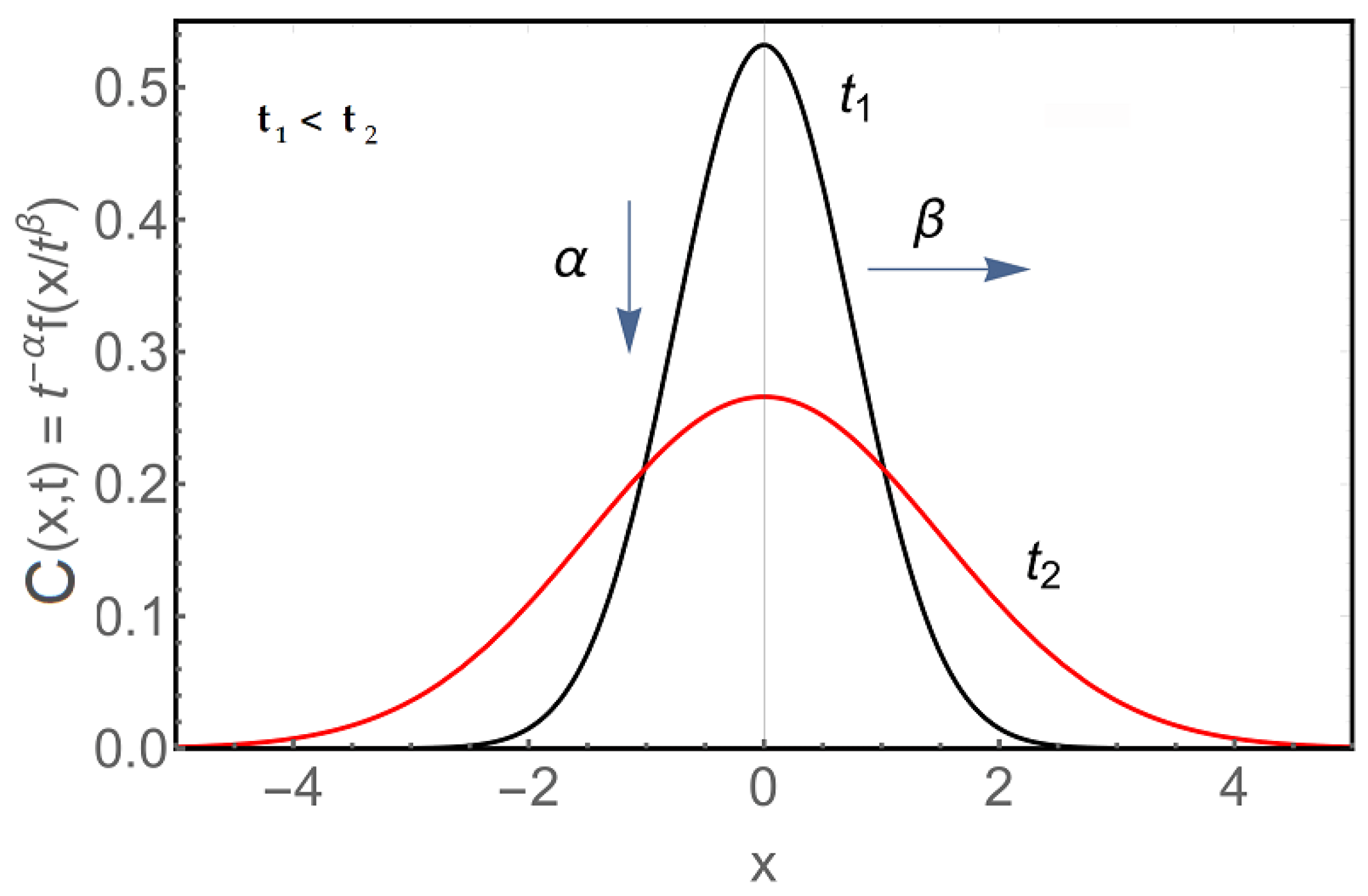
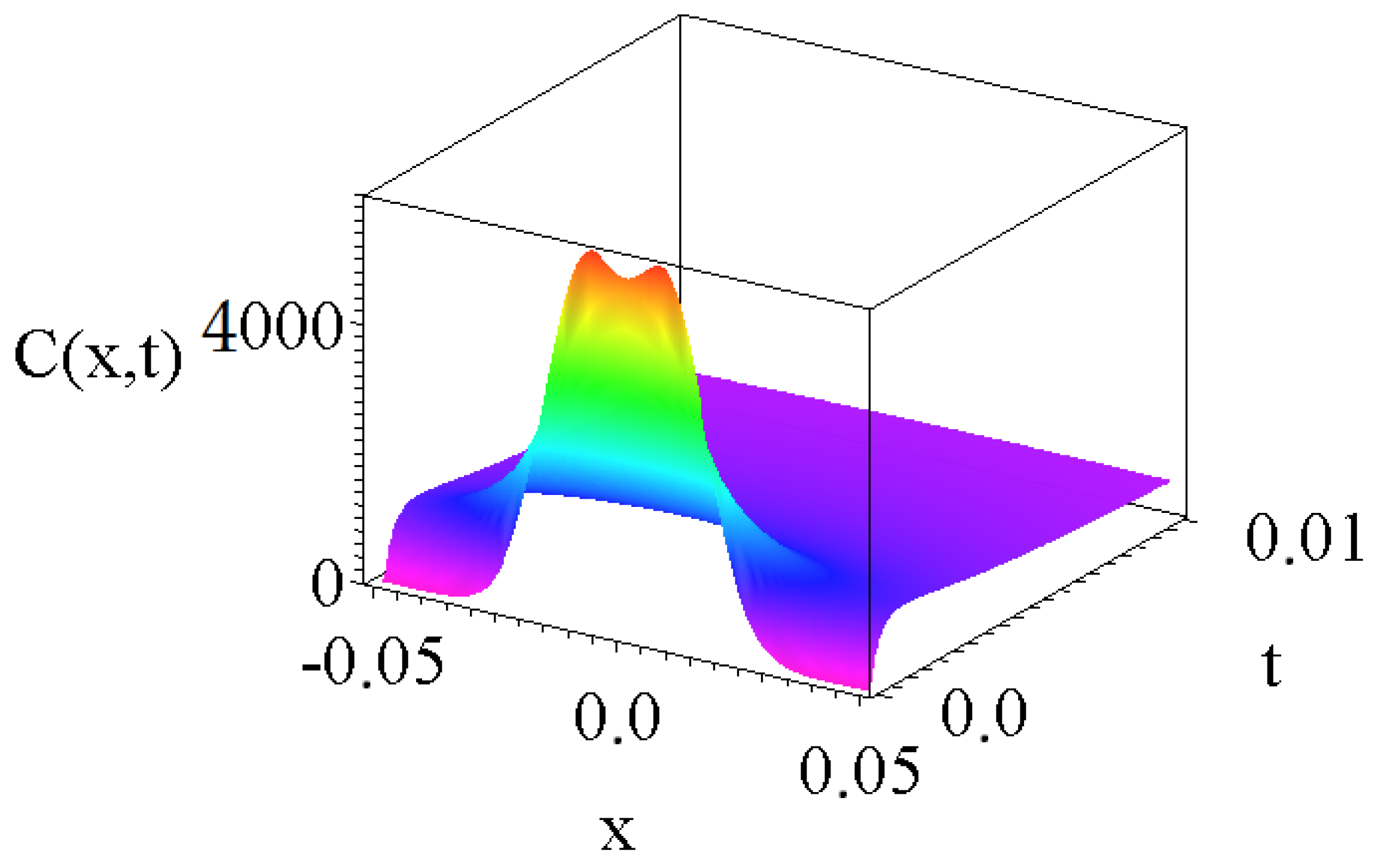
2. Theory and Results

In the case of infinite horizon, when we want to derive the corresponding solutions, we make the following self-similar transformation:
C ( x , t ) = t α f x t β = t α f ( η ) .
Note that the spatial coordinate x now runs along the whole real axis. The role of α and β is illustrated on Figure 1. As is indicated in the figure, β shows the spreading and α the decay in time.
This kind of Ansatz has been applied by Sedov [39], and was later also used by Raizer and Zel’dowich [40] For certain systems, Barenblatt applied it successfully [41] as well. We have also used it for linear or non-linear partial differential equation (PDE) systems, which are from fluid mechanics [42,43,44] or quantum mechanical systems [45]. In certain cases, the equation of state of the fluid also plays a role [46,47]. Diffusion-related applications of the self-similar analysis method can be found in relatively recent works as well [48,49,50].
The transformation takes into account the (4) formula, and before the function f, instead of 1 / t there is a generalized function 1 / t α , and in the argument of f, the fraction x / t β is possible, with a β which should be determined later.
We evaluate the first and second derivative of relation (5), and insert it in the equation of diffusion (1). This yields the following ordinary differential equation (ODE)
α t α 1 f ( η ) β t α 1 η d f ( η ) d η = D t α 2 β d 2 f ( η ) d η 2 .
The reasoning is self-consistent if all three terms have the same decay in time. This is possible if
α = arbitrary real number , β = 1 / 2 ,
and yields the following ODE
α f 1 2 η f = D f .
This ODE is a kind of characteristic equation, with the above-presented change of variable. One can observe that for α = 1 / 2 , this equation can be written as
1 2 η f = D f .
If this equation is integrated once
Const 0 1 2 η f = D f ,
where Const 0 is an arbitrary constant, which may depend on certain conditions related to the problem. If we take this Const 0 = 0 , then one arrives to the generic solution
f = f 0 e η 2 4 D ,
where f 0 is a constant. Inserting this form of f in form of C ( x , t ) given by Equation (5)—for α = 1 / 2 as it was mentioned earlier—one obtains an even solution for the space variable:
C ( x , t ) = f 0 1 t 1 2 e x 2 4 D t .
By this, we have recovered the generic Gaussian solution, which can be seen in Figure 2a.
If we want to find further solutions, the Equation (8) has to be solved for general α . The general solution for infinite horizon of (8) can be written as:
f ( η ) = η · e η 2 4 D c 1 M 1 α , 3 2 , η 2 4 D + c 2 U 1 α , 3 2 , η 2 4 D ,
where c 1 and c 2 are real integration constants, which are fixed by the initial conditions, and M ( , , ) and U ( , , ) are the Kummer’s functions. For exhaustive details, consult [51].
If α are positive integer numbers, then both special functions M and U are finite polynomials in terms of the third argument η 2 4 D
f ( η ) = η · e η 2 4 D κ 0 + κ 1 η 2 4 D + + κ n 1 · η 2 4 D n 1 .
These give the odd solutions of the diffusion equation for α = n , (where n positive integer), in terms of the space variable. It follows for the complete solution C ( x , t )
C ( x , t ) = 1 t n f ( η ) = 1 t n x t e x 2 4 D t · κ 0 + κ 1 x 2 4 D t + + κ n 1 · x 2 4 D t n 1 .
These odd solutions have been studied thoroughly by Mátyás and Barna in previous works [10,11] and for completeness, we present these solutions in Appendix A.
For the even solutions, we denote by g ( η ) the following function
f ( η ) = η · e η 2 4 D g ( η ) ,
Inserting this equation into Equation (8), we have
η g + 2 g η 2 2 D g + ( α 1 ) η D g = 0 .
In concordance with Equation (13), we get the general solution
g ( η ) = c 1 M 1 α , 3 2 , η 2 4 D + c 2 U 1 α , 3 2 , η 2 4 D .
At this point, we make the conjecture from the forms of U and M, that if we had the classical spatially even solution for α = 1 / 2 , than the next spatially even solution would be for α = 3 / 2 , with the form of g
g ( η ) = K 0 1 η + K 1 η ,
where K 0 and K 1 are arbitrary constants, which should be determined later. We insert this form of g in (17); we find that the form (19) fulfills the Equation (17) if
K 1 = 1 2 D K 0 .
We obtain the same result if we insert the form
f ( η ) = η · e η 2 4 D K 0 1 η + K 1 η ,
directly into the Equation (8). By this, for α = 3 / 2 , we get for the function f
f ( η ) = K 0 · η · e η 2 4 D 1 η 1 2 D η = K 0 · e η 2 4 D 1 1 2 D η 2 .
Substituting this form into (5), one gets
C ( x , t ) = K 0 1 t 3 2 e x 2 4 D t 1 1 2 D x 2 t .
This result is visualized in Figure 2b.
If we follow the case α = 5 / 2 = 2.5 , then the following form for the function g ( η ) can be considered
g ( η ) = K 0 · 1 η + K 1 · η + K 2 · η 3 .
If we insert this form in the Equation (17), the following relations for the constants K 0 , K 1 and K 2 can be derived
K 1 = K 0 D ,
and
K 2 = K 1 12 D = K 0 12 D 2 .
By this, we get for the g ( η )
g ( η ) = K 0 1 η 1 D η + 1 12 D 2 η 3 .
Correspondingly the final form for f ( η ) for α = 2.5 is
f ( η ) = K 0 · e η 2 4 D 1 1 D η 2 + 1 12 D 2 η 4 .
Inserting this form into (5), one gets
C ( x , t ) = K 0 1 t 5 2 e x 2 4 D t 1 1 D x 2 t + 1 12 D 2 x 4 t 2 .
This result can be seen in Figure 2c.
If we follow the case α = 7 / 2 = 3.5 , then the following form for the function g ( η ) can be considered:
g ( η ) = K 0 · 1 η + K 1 · η + K 2 · η 3 + K 3 · η 5 .
If we replace this form into Equation (17), the next relations among the constants K 0 , K 1 , K 2 and K 3 can be derived:
K 1 = 3 2 K 0 D ,
for the next coefficient
K 2 = K 1 6 D = K 0 4 D 2 .
Finally, for the third coefficient one obtains
K 3 = K 2 30 D = K 0 120 D 3 .
Inserting these coefficients into the Formula (30), one obtains the following expression
g ( η ) = K 0 1 η 3 2 D · η + 1 4 D 2 · η 3 1 120 D 3 · η 5 .
This form of g yields, by Equation (16), for the function f
f ( η ) = K 0 · e η 2 4 D 1 3 2 D η 2 + 1 4 D 2 η 4 1 120 D 3 η 6 .
Inserting this form into (5), one obtains
C ( x , t ) = K 0 1 t 7 2 e x 2 4 D t 1 3 2 D x 2 t + 1 4 D 2 x 4 t 2 1 120 D 3 x 6 t 3 .
This result is clearly visualized in Figure 2d.
It is evident that by including higher terms in the finite series of Equation (30), the solutions for α = 9 / 2 , 11 / 2 , etc. can be evaluated in a direct way.
For completeness, we present the shape functions f ( η ) s on Figure 3. Note that solutions with higher α values have more oscillations and quicker decay. The same features appear for odd solutions as well.
As we can see, at this point, the solutions fulfills the boundary condition C ( ) 0 if x ± , for positive α values.
The general initial value problem can be solved with the usage of the Green’s functions formalism. According to the standard theory of the Green’s functions, the solution of the diffusion Equation (1) can be obtained via the next convolution integral:
C ( x , t ) = 1 2 π t + w ( x 0 ) G ( x x 0 ) d x 0 ,
where w ( x 0 ) defines the initial condition of the problem, C | t = 0 = w ( x 0 ) . The Green’s function for diffusion is well defined and can be found in many mathematical textbooks e.g., [52,53,54,55]:
G ( x x 0 ) = e x p ( x x 0 ) 2 4 t D .
On the other side, the Gaussian function is a fundamental solution of diffusion.
We will see in the following that for some special forms of the initial conditions, such as polynomials, Gaussian, Sinus or Cosines, the convolution integral can be done analytically.
In the following, we evaluate the convolution integral for α = 1 / 2 .
As an example for the initial condition problem, we may consider the following smooth function with a compact support:
w ( x 0 ) = Heaviside ( 3 x 0 ) · Heaviside ( 3 + x 0 ) · ( 9 x 0 2 ) 9 .
This initial condition is a typical initial distribution for diffusion, and one can see on Figure 4a.
The convolution integral for α = 1 / 2 :
C ( x , t ) = 1 2 π t + Heaviside ( 3 x 0 ) · Heaviside ( 3 + x 0 ) · ( 9 x 0 2 ) 9 · e ( x x 0 ) 2 4 D t d x 0 .
The result of this evaluation is
C ( x , t ) = 1 2 π t [ π t erf 3 + x 2 t + 2 9 x t e 6 x + x 2 + 9 4 t + 2 3 t e 6 x + x 2 + 9 4 t 2 9 t 3 2 π erf 3 + x 2 t 1 9 x 2 π t erf 3 + x 2 t π t erf x 3 2 t 2 9 x t e 6 x + x 2 + 9 4 t + 2 3 t e 6 x + x 2 + 9 4 t + 2 9 t 3 2 π erf x 3 2 t + 1 9 x 2 π t erf x 3 2 t ] ,
which is presented on Figure 4b.

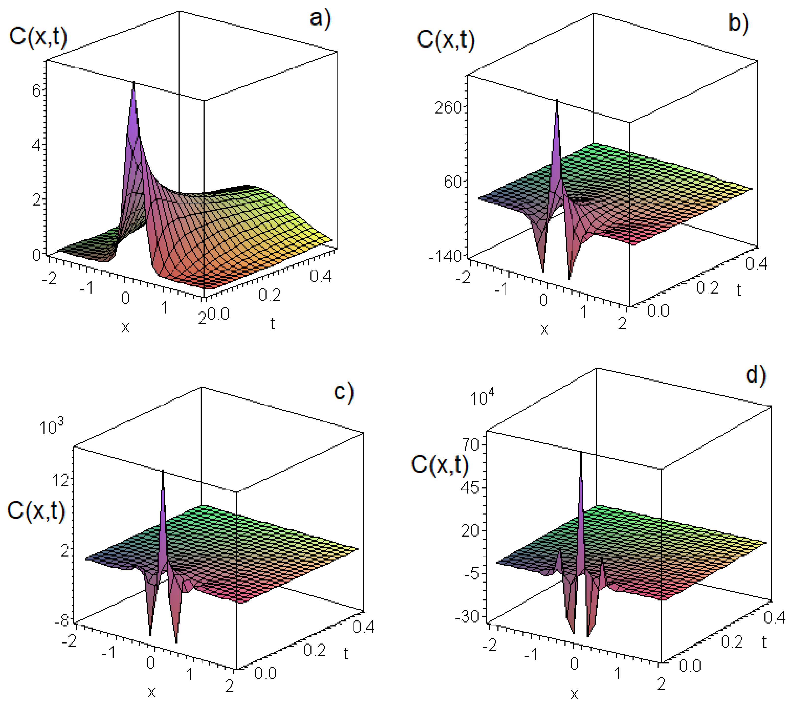
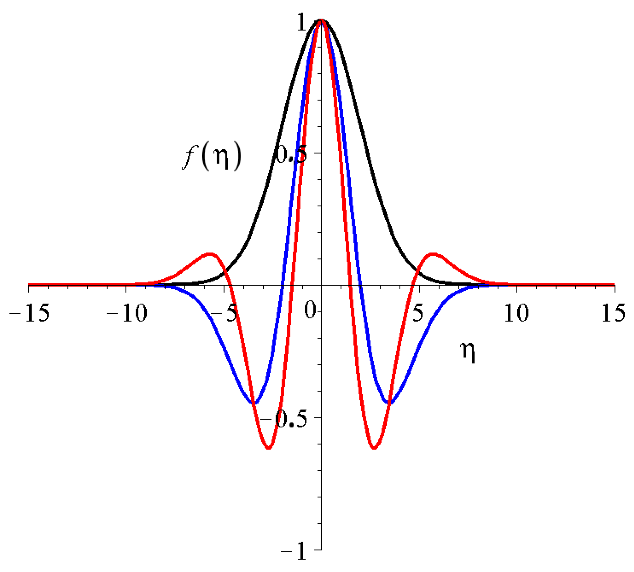
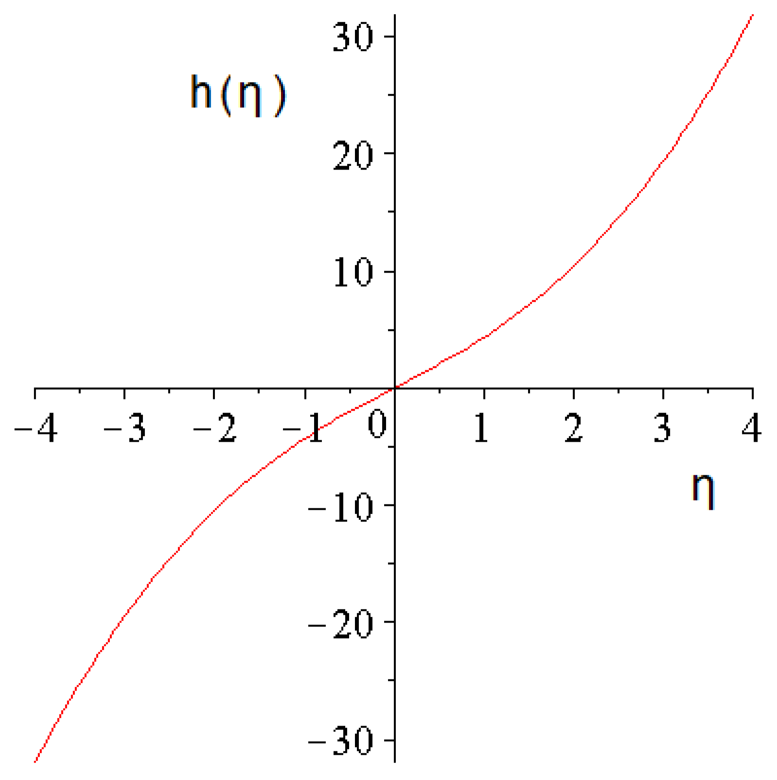
3. The Properties of the Shape Functions and Solutions

In the following, we study some properties of the shape functions f ( η ) and of the complete solutions C ( x , t ) . First, we consider the L 1 integral norms.
For the case α = 1 / 2 the form of
f ( η ) d η = f 0 e η 2 4 D d η = f 0 2 π D .
The constant f 0 is chosen, depending on the problem. If C stands for the density which diffuses, f 0 in the above integral is related to the total mass of the system.
Correspondingly,
C ( x , t ) d x = f 0 1 t e x 2 4 D t d x = f 0 2 π D .
For the case α = 3 / 2 :
f ( η ) d η = K 0 · e η 2 4 D 1 1 2 D η 2 d η = 0 .
It is interesting to see that the integral of first even shape function beyond Gaussian is zero. An even more remarkable feature is, however, that
0 f ( η ) d η = 0 f ( η ) d η = 0 .
So the oscillations, the positions of the zero transitions, divide the function in such a way that the integral is not only on the whole real axis ( ) but on the half axis ( 0 ) or ( 0 ) gives zero as well.
Evaluating the same type of integrals for the corresponding solution C ( x , t ) , we have
C ( x , t ) d x = 0 C ( x , t ) d x = 0 C ( x , t ) d x = K 0 · 1 t 3 / 2 e x 2 4 D t 1 1 2 D x 2 t d x = 0 ,
at any time point, (and for any diffusion coefficient D).
The same property is true for all possible higher harmonic solutions if α is positive half-integer number α = ( 2 n + 1 ) / 2 when ( n ϵ N ). This property has far-reaching consequences. The linearity of the regular diffusion equation and this additional property of this even series of solutions makes it possible to perturb the usual Gaussian in such a way that the total number of particles is conserved during the diffusion process; however, the initial distribution can be changed significantly. One can see from the final form of the solutions C ( x , t ) α 1 t α that the decay of these perturbations are, however, short-lived because they have a quicker decay than the standard Gaussian solutions. For completeness, we present a C ( x , t ) solution which is a linear combination of the first two even solutions α = 1 / 2 , 3 / 2 in the form of
C ( x , t ) = 60 t 1 2 e x 2 4 t 0.001 t 3 2 e x 2 4 t 1 x 2 2 t ,
on Figure 5. Note that coefficients with different orders of magnitude have to be applied to reach a visible effect when the sum of two functions have to be visualised with different power-law decay.
As a second property, we investigate the cosine Fourier transform of the shape functions:
C α ( k ) = C o s ( k · η ) f α ( η ) d η .
It can be shown with direct integration that the Fourier transform is
C α = 2 N + 1 2 ( k ) l · π · k 2 N · D N · e k 2 D 1 D ,
for all N ϵ N \ 0 positive integer and l is a real constant. This means that qualitatively, the spectra for all positive half integer α are similar. They start from zero, have a global positive maximum and a quick decay to zero. It is generally known from spectral analysis that pulses of finite length have band spectra which have a minimal, a maximal and a central frequency.
In Appendix A, the corresponding normalization coefficients are given for the odd functions as well.

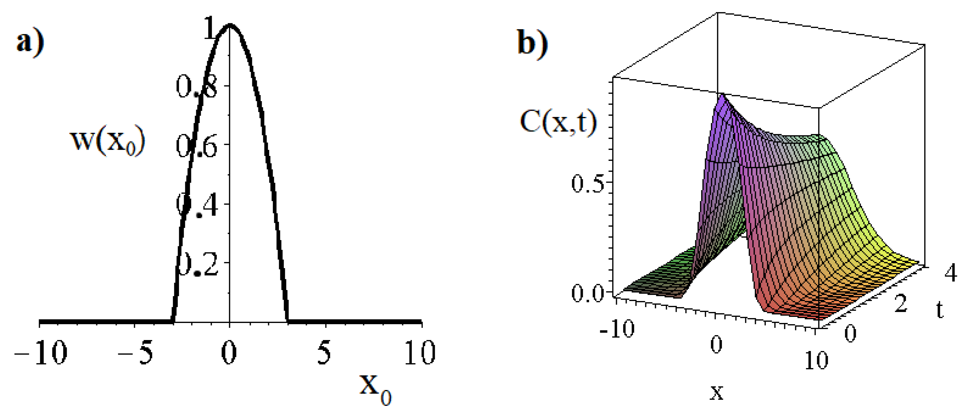
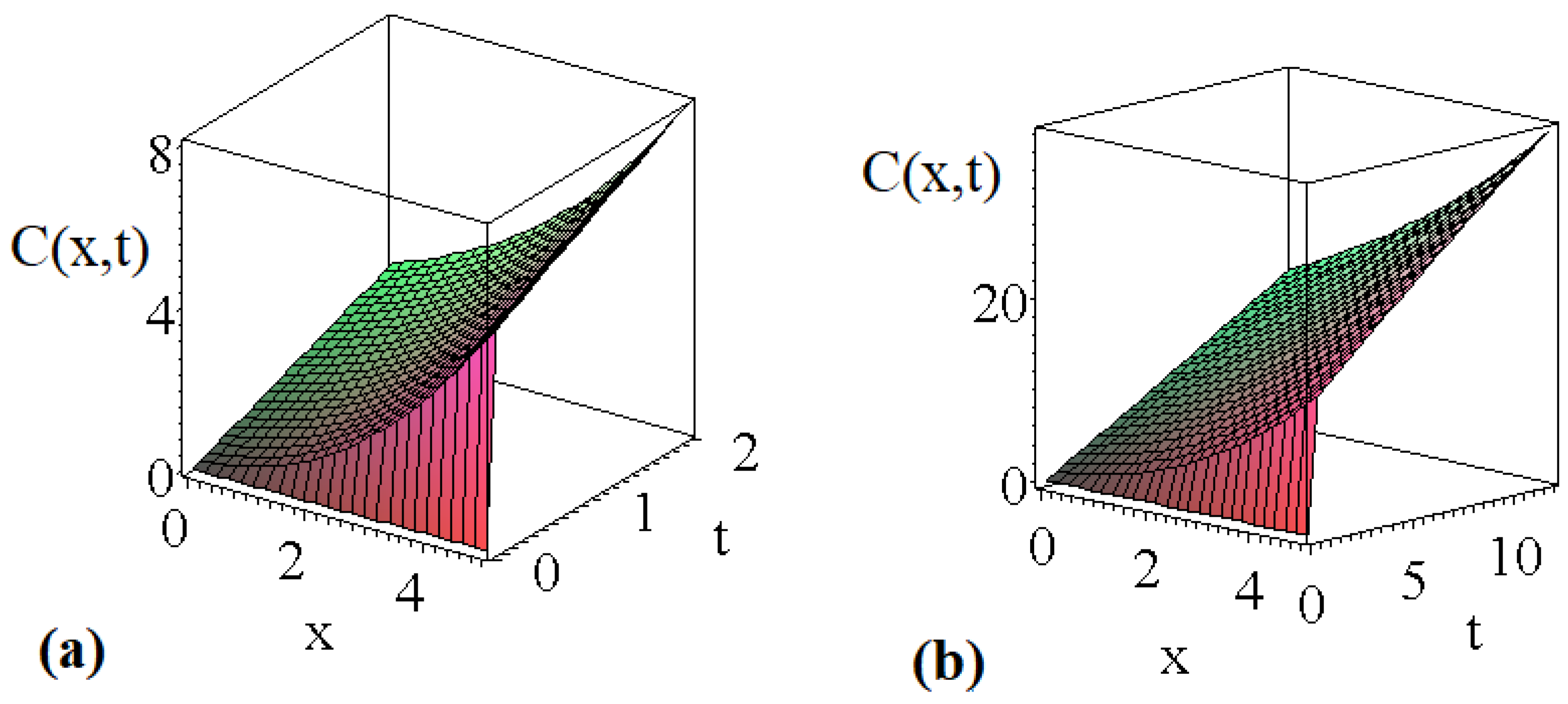
4. The Diffusion Equation with Constant Source

At this point we try to find solutions of the diffusion equation, mainly with the self similar Ansatz, where on the right hand side, there is a constant source term:
C ( x , t ) t = D 2 C ( x , t ) x 2 + n .
For this equation, one also apply the self-similar transformation (5), and we get a modified equation relative to the homogeneous one
α t α 1 f ( η ) β t α 1 η d f ( η ) d η = D t α 2 β d 2 f ( η ) d η 2 + n .
The free term on the r.h.s. has no explicit time decay; consequently, we expect the same from the other terms, which means
α 1 = 0
α 2 β = 0 .
The two equations have to be fulfilled simultaneously. Solving these equations, we get the following values for α and β :
α = 1 and β = 1 2
Inserting these values to the Equation (50), we get the following ODE
f ( η ) 1 2 η d f ( η ) d η = D d 2 f ( η ) d η 2 + n .
We emphasize that we arrived to this equation by a self-similar transformation. At this point, we observe that if we shift the function f by a constant, and introduce the function h:
h ( η ) = f ( η ) n
we arrive to a slightly modified equation
h ( η ) 1 2 η d h ( η ) d η = D d 2 h ( η ) d η 2 .
One may observe that if the transformation η η and h ( η ) = h ( η ) is applied, the equation still remains the same; consequently, we expect at least one even solution.
If we look for the even solution by polynomial expansion,
h ( η ) = A + B η 2 +
then, we get by direct substitution
A = 2 · B · D .
This means that the even solution reads as follows
h ( η ) = B ( 2 D + η 2 )
where B is a constant depending on initial conditions.
Furthermore, we observe that the transformation η η and h ( η ) = h ( η ) also leaves Equation (56) unchanged. This means that it is worthwhile to look for an odd solution as well. The odd solution of the equation is
h ( η ) = 2 D η e η 2 4 D + π ( 2 D 3 / 2 + D η 2 ) e r f 1 2 η D
One can see the form of this odd solution in Figure 6.
We mention, that Equation (56) may have a further solution, which eventually does not have the symmetry to be even or odd, and that may be expressed in terms of a Hermite function with a negative integer as one can see in Equation (8) of the Reference [11]. Such a solution reads as follows
h ( η ) = e η 2 4 D · H e r m i t e [ 3 , η 2 D ]
We try to find certain relevant features of this result. In an interesting way, the series expansion of the above solution (61) means a sum of an even function with second order and another odd function, which appears to be proportional to the series of solution (60). The first terms of these series are presented in Appendix B.
If n is positive in the Equation (49), then we can talk about a source in the equation, and if n is negative, than we say that there is a sink in the diffusion process. The sink can be considered physical by the time C ( x , t ) 0 . Diffusive systems with sinks have been studied in ref. [56], and water purification by adsorption also means a process with change of concentration in space and decrease in time [57].
A general solution for the shape function can be obtained from the linear combination of the even and odd solutions presented above
h ( η ) = κ 1 2 D η e η 2 4 D + π ( 2 D 3 / 2 + D η 2 ) e r f 1 2 η D + κ 2 [ 2 D + η 2 ]
where κ 1 and κ 2 are constants depending on the initial or boundary conditions of the problem.
Inserting this shape function to the general solution (5), we get for the final form of C ( x , t ) in the presence of a constant source
C ( x , t ) = t · κ 1 2 D x t e x 2 4 D t + π 2 D 3 / 2 + D x 2 t e r f 1 2 x D t + κ 2 2 D + x 2 t + n
For relatively shorter times, the general solution has interesting features depending on the weight of the even or the odd part of the solution, as one can see in Figure 7a.
The long time behavior is dominated by the constant of the even solution and the source term. Correspondingly, for sufficiently long times, the relation C ( x , t ) ( 2 κ 2 D + n ) · t characterizes the dynamics, as one can see in Figure 7b.

5. Summary and Outlook

Applying the well-known self-similar Ansatz—together with an additional change of variables—we derived symmetric solutions for the one-dimensional diffusion equations. Using the Fourier series analogy, we might say that these solutions may be considered as possible higher harmonics of the fundamental Gaussian solution. As unusual properties, we found that the integral of these solutions—beyond Gaussian—gives zero on both the half and the whole real axis as well. Thanks to the linearity of the diffusion equation, these kinds of functions can be added to the particle- (or energy-) conserving fundamental Gaussian solution; therefore, a new kind of particle diffusion process can be described. Due to the higher α self-similar exponents, these kinds of solutions give relevant contributions only at smaller time coordinates, because the corresponding solutions decay more quickly than the usual Gaussian solution. In case of a constant source or sink term in the diffusion equation, the value of α is no more arbitrary; it has a constant value α = 1 . Even for this fixed value of α , the diffusion equation with source term has even and odd solutions as well.
These kinds of solutions can also be evaluated for two- or three-dimensional, cylindrical or spherical symmetric systems as well. Work is in progress to apply this kind of analysis to more sophisticated diffusion systems as well. We hope that our new solutions have far-reaching consequences and that they will be successfully applied in other scientific disciplines such as quantum mechanics, quantum field theory, astrophysics, probability theory or in financial mathematics in the near future.

Author Contributions

Methodology, original draft and validation, L.M.; conceptualization, investigation and software, I.F.B. All authors have read and agreed to the published version of the manuscript.

Funding

There was no extra external funding.

Data Availability Statement

The data that support the findings of this study are all available within the article.

Conflicts of Interest

The authors declare no conflict of interest.

Appendix A

For completeness and for direct comparison, we show the first five odd shape functions f ( η ) and the corresponding solutions C ( x , t ) :
f ( η ) = e r f η 2 D , f ( η ) = κ 0 · η · e η 2 4 D , f ( η ) = κ 0 · η · e η 2 4 D · 1 1 6 D η 2 , f ( η ) = κ 0 · η · e η 2 4 D · 1 1 3 D η 2 + 1 60 1 D 2 η 4 , f ( η ) = κ 0 · η · e η 2 4 D · 1 1 2 D η 2 + 1 20 1 D 2 η 4 1 840 1 D 3 η 6 ,
for α = 0 , 1 , 2 , 3 , 4 N . The first case with the change of variable x / t with no α (or implicitly α = 0 ) dates back to Boltzmann [58], as is also mentioned by [59,60].
All integrals of the functions from (A1) on the whole real axis give zero:
f α ( η ) d η = 0 ,
However, on the half-axis:
0 f α = 0 ( η ) d η = ,
and for additional non-zero integer α s, we get:
0 f α ( η ) d η = D α 1 / 2 .
Integrals on the opposite half-axis ( 0 ] have the same value with a negative sign, respectively. The forms for odd C ( x , t ) s are the following:
C ( x , t ) = e r f x 2 D t , C ( x , t ) = κ 1 x t 3 2 e x 2 4 D t , C ( x , t ) = κ 1 x t 5 2 e x 2 4 D t 1 x 2 6 D t , C ( x , t ) = κ 1 x t 7 2 e x 2 4 D t 1 x 2 3 D t + x 4 60 ( D t ) 2 , C ( x , t ) = κ 1 x t 9 2 e x 2 4 D t 1 x 2 2 D t + x 4 20 ( D t ) 2 x 6 840 ( D t ) 3 .
The space integrals of C α ( x , t ) d x = 0 for all positive integers α s. On the positive half-axis for α = 0 , the integral of the error function in infinite, for positive α a, it is:
C α ( x , t ) = D t 1 2 α α 1 2 .
which are well-defined values for finite, D, t and α . On the ( 0 ] half axis, the sign is opposite. Additional detailed analysis of the odd functions was presented in our former study [11].

Appendix B

The power series of the Equation (61) reads as follows
e η 2 4 D · H e r m i t e [ 3 , η 2 D ] = π 8 η 4 D + π η 2 16 D η 3 48 D 3 / 2 + η 5 1920 D 5 / 2 η 7 53760 D 7 / 2 + o ( η 9 ) = π 8 + π 16 η 2 D + 1 16 4 η D 1 3 η 3 D 3 / 2 + 1 120 η 5 D 5 / 2 1 3360 η 7 D 7 / 2 + o ( η 9 ) .
The series of relation (60) yields the following
2 D η e η 2 4 D + π ( 2 D 3 / 2 + D η 2 ) e r f 1 2 η D = = D 3 / 2 4 η D + 1 3 η 3 D 3 / 2 1 120 η 5 D 5 / 2 + 1 3360 η 7 D 7 / 2 + o ( η 9 ) .
As one can see—based on power expansions—the solution related to the Hermite function (A7) is still a kind of linear combination of the quadratic even solution and the odd solution (A8).

References

  1. Crank, J. The Mathematics of Diffusion; Clarendon Press: Oxford, UK, 1956. [Google Scholar]
  2. Ghez, R. Diffusion Phenomena; Dover Publication: Mineola, NY, USA, 2001. [Google Scholar]
  3. Bennett, T.D. Transport by Advection and Diffusion: Momentum, Heat and Mass Transfer; John Wiley & Sons: Hoboken, NJ, USA, 2013. [Google Scholar]
  4. Lienhard, J.H., IV; Lienhard, J.H., V. A Heat Transfer Textbook, 4th ed.; Phlogiston Press: Cambridge, MA, USA, 2017. [Google Scholar]
  5. Newman, J.; Battaglia, V. The Newman Lectures on Transport Phenomena; Jenny Stanford Publishing: Dubai, United Arab Emirates, 2021. [Google Scholar]
  6. Kardar, M.; Parisi, G.; Zhang, Y.-C. Dynamic scaling of growing interfaces. Phys. Rev. Lett. 1986, 56, 889. [Google Scholar] [CrossRef]
  7. Barna, I.F.; Bognár, G.; Guedda, M.; Hriczó, K.; Mátyás, L. Analytic self-similar solutions of the Kardar-Parisi-Zhang interface growing equation with various noise terms. Math. Model. Anal. 2020, 25, 241. [Google Scholar] [CrossRef]
  8. Barabási, A.L.; Stanley, E. Fractal Concepts in Surface Growth; Cambridge University Press: Cambridge, MA, USA, 1995. [Google Scholar]
  9. Mátyás, L.; Gaspard, P. Entropy production in diffusion-reaction systems: The reactive random Lorentz gas. Phys. Rev. E 2005, 71, 036147. [Google Scholar] [CrossRef] [PubMed]
  10. Mátyás, L.; Barna, I.F. General self-similar solutions of diffusion equation and related constructions. Rom. J. Phys. 2022, 67, 101. [Google Scholar]
  11. Barna, I.F.; Mátyás, L. Advanced Analytic Self-Similar Solutions of Regular and Irregular Diffusion Equations. Mathematics 2022, 10, 3281. [Google Scholar] [CrossRef]
  12. Cannon, J.R. The One-Dimensional Heat Equation; Addison-Wesley Publishing: Reading, MA, USA, 1984. [Google Scholar]
  13. Cole, K.D.; Beck, J.V.; Haji-Sheikh, A.; Litkouhi, B. Heat Conduction Using Green’s Functions; Series in Computational and Physical Processes in Mechanics and Thermal Sciences (2nd ed); CRC Press: Boca Raton, FL, USA, 2011. [Google Scholar]
  14. Mátyás, L.; Tél, T.; Vollmer, J. Thermodynamic cross effects from dynamical systems. Phys. Rev. E 2000, 61, R3295. [Google Scholar] [CrossRef]
  15. Thambynayagam, R.K.M. The Diffusion Handbook: Applied Solutions for Engineers; McGraw-Hill: New York, NY, USA, 2011. [Google Scholar]
  16. Michaud, G.; Alecian, G.; Richer, G. Atomic Diffusion in Stars; Springer: New York, NY, USA, 2013; Volume 70. [Google Scholar]
  17. Murray, J.D. Mathematical Biology II: Spatial Models and Biomedical Applications, 3rd ed.; Springer: New York, NY, USA, 2003. [Google Scholar]
  18. Alebraheem, J. Predator interference in a predator-prey model with mixed functional and numerical responses. Hindawi J. Math. 2023, 2023, 4349573. [Google Scholar] [CrossRef]
  19. Perthame, B. Parabolic Equations in Biology; Springer International Publishing: Berlin/Heidelberg, Germany, 2015. [Google Scholar]
  20. Szép, R.; Mateescu, E.; Nechifor, A.C.; Keresztesi, Á. Chemical characteristics and source analysis on ionic composition of rainwater collected in the Charpatians “Cold Pole”, Ciuc basin, Eastern Carpatians, Romania. Environ. Sci. Pollut. Res. 2017, 24, 27288. [Google Scholar] [CrossRef] [PubMed]
  21. Gillespie, D.T.; Seitaridou, E. Simple Brownian Diffusion; Oxford University Press: Oxford, UK, 2013. [Google Scholar]
  22. Tálos, K.; Páger, C.; Tonk, S.; Majdik, C.; Kocsis, B.; Kilár, F.; Pernyeszi, T. Cadmium biosorption on native Saccharomyces cerevisiae cells in aqueous suspension. Acta Univ. Sapientiae Agric. Environ. 2009, 1, 20. [Google Scholar]
  23. Nechifor, G.; Voicu, S.I.; Nechifor, A.C.; Garea, S. Nanostructured hybrid membrane polysulfone-carbon nanotubes for hemodialysis. Desalination 2009, 241, 342. [Google Scholar] [CrossRef]
  24. Lv, J.; Ren, K.; Chen, Y. CO2 diffusion in various carbonated beverages: A molecular dynamic study. Phys. Chem. 2018, 122, 1655. [Google Scholar] [CrossRef]
  25. Hägerstrand, T. Innovation Diffusion as a Spatial Process; The University of Chicago Press: Chicago, IL, USA, 1967. [Google Scholar]
  26. Rogers, E.M. Diffusion of Innovations; The Free Press: Los Angeles, CA, USA, 1983. [Google Scholar]
  27. Nakicenovic, N.; Griübler, A. Diffusion of Technologies and Social Behavior; Springer: Berlin/Heidelberg, Germany, 1991. [Google Scholar]
  28. Bunde, A.; Kärger, J.C.; Vogl, G. Diffusive Spreading in Nature, Technology and Society; Springer: Berlin/Heidelberg, Germany, 2018. [Google Scholar]
  29. Vogel, G. Adventure Diffusion; Springer: Berlin/Heidelberg, Germany, 2019. [Google Scholar]
  30. Mazzoni, T. A First Course in Quantitative Finance; Cambridge University Press: Cambridge, MA, USA, 2018. [Google Scholar]
  31. Lázár, E. Quantifying the economic value of warranties: A survey. Acta Univ. Sapientiae Econ. Bus. 2014, 2, 75. [Google Scholar] [CrossRef]
  32. Albert, R.; Barabási, A.-L. Statistical mechanics of complex networks. Rev. Mod. Phys. 2002, 74, 47. [Google Scholar] [CrossRef]
  33. Rogolino, P.; Kovács, R.; Ván, P.; Cimmelli, V.A. Generalized heat-transport equations: Parabolic and hyperbolic models. Contin. Mech. Thermodyn. 2018, 30, 1245. [Google Scholar] [CrossRef]
  34. Jalghaf, H.K.; Kovács, E.; Majár, J.; Nagy, A.; Askar, A.H. Explicit stable finite difference methods for diffusion-reaction type equations. Mathematics 2021, 9, 3308. [Google Scholar] [CrossRef]
  35. Nagy, A.; Saleh, M.; Omle, I.; Kareem, H.; Kovács, E. New stable, explicit shifted-hopscotch algoritms for the heat equation. Math. Comput. Appl. 2021, 26, 61. [Google Scholar]
  36. Ezzahri, Y.; Ordonez-Miranda, J.; Joulain, K. Heat transport in semiconductor crystals under large temperature gradients. Int. J. Heat Mass Transf. 2017, 108, 1357. [Google Scholar] [CrossRef]
  37. Cussler, E.L. Diffusion: Mass Transfer in Fluid Systems, 3rd ed.; Cambridge University Press: Cambridge, MA, USA, 2009. [Google Scholar]
  38. Bluman, G.W.; Cole, J.D. The general similarity solution of the heat equation. J. Math. Mech. 1969, 18, 1025. [Google Scholar]
  39. Sedov, L. Similarity and Dimensional Methods in Mechanics; CRC Press: Boca Raton, FL, USA, 1993. [Google Scholar]
  40. Zel’dovich, Y.B.; Raizer, Y.P. Physics of Shock Waves and High Temperature Hydrodynamic Phenomena; Academic Press: New York, NY, USA, 1966. [Google Scholar]
  41. Baraneblatt, G.I. Similarity, Self-Similarity, and Intermediate Asymptotics; Consultants Bureau: New York, NY, USA, 1979. [Google Scholar]
  42. Barna, I.F.; Mátyás, L. Analytic solutions for the three dimensional compressible Navier-Stokes equation. Fluid Dyn. Res. 2014, 46, 055508. [Google Scholar] [CrossRef]
  43. Barna, I.F.; Pocsai, M.A.; Lökös, S.; Mátyás, L. Rayleigh-Benard convection in the generalized Oberbeck-Boussinesq system. Chaos Solitons Fractals 2017, 103, 336. [Google Scholar] [CrossRef]
  44. Barna, I.F.; Pocsai, M.A.; Barnaföldi, G.G. Self-similar solutions of a gravitating dark fluid. Mathematics 2022, 10, 3220. [Google Scholar] [CrossRef]
  45. Barna, I.F.; Pocsai, M.A.; Mátyás, L. Analytic solutions of the Madelung equation. J. Gen. Lie Theory Appl. 2017, 11, 1000271. [Google Scholar]
  46. Csanád, M.; Vargyas, M. Observables from a solution of (1+3)-dimensional relativistic hydrodynamics. Eur. Phys. J. A 2010, 44, 473. [Google Scholar] [CrossRef]
  47. Barna, I.F.; Mátyás, L. Analytic solutions for the one-dimensional compressible Euler equation with heat conduction closed with different kind of equation of states. Miskolc Math. Notes 2013, 14, 785. [Google Scholar] [CrossRef]
  48. Nath, G.; Singh, S. Approximate analytical solution for shock wave in rotational axisymetric perfect gas with azimutal magnetic field: Isotermal flow. J. Astrophys. Astron. 2019, 40, 50. [Google Scholar] [CrossRef]
  49. Sahu, P.K. Shock wave driven out by a piston in a mixture of a non-ideal gas and small solid particles under the influence of azimuthal or axial magnetic field. Braz. J. Phys. 2020, 50, 548. [Google Scholar] [CrossRef]
  50. Kanchana, C.; Su, Y.; Zhao, Y. Primary and secondary instabilities in Rayleigh-Benard convention of water-copper nanoliquid. Commun. Nonlinear Sci. Numer. Simul. 2020, 83, 105129. [Google Scholar] [CrossRef]
  51. Olver, F.W.J.; Lozier, D.W.; Boisvert, R.F.; Clark, C.W. NIST Handbook of Mathematical Functions; Cambridge University Press: Cambridge, MA, USA, 2010. [Google Scholar]
  52. Kythe, P.K. Green’s Functions and Linear Differential Equations; Chapman & Hall/CRC Applied Mathematics and Nonliner Science; CRC Press: Boca Raton, FL, USA, 2011. [Google Scholar]
  53. Rother, T. Green’s Functions in Classical Physics; Lecture Notes in Physics; Springer International Publishing: New York, NY, USA, 2017; Volume 938. [Google Scholar]
  54. Bronshtein, I.N.; Semendyayev, K.A.; Musiol, G.; Mühlig, H. Handbook of Mathematics; Springer: Wiesbaden, Germany, 2007. [Google Scholar]
  55. Greiner, W.; Reinhardt, J. Quantum Electrodynamics; Springer: Berlin/Heidelberg, Germany, 2009. [Google Scholar]
  56. Claus, I.; Gaspard, P. Fractals and dynamical chaos in a two-dimensional Lorentz gas with sinks. Phys. Rev. E 2001, 63, 036227. [Google Scholar] [CrossRef]
  57. Rápó, E.; Tonk, S. Factors affecting synthetic dye adsorption; desorption studies: A review of results from the last five years (2017–2021). Molecules 2021, 26, 5419. [Google Scholar] [CrossRef]
  58. Boltzmann, L. Zur Intergration der Diffusionsgleichung bei variabeln Diffusionscoefficienten. Ann. Phys. 1894, 53, 959. [Google Scholar] [CrossRef]
  59. Lonngren, K.E. Self similar solution of plasma equations. Proc. Indian Acad. Sci. 1977, 86, 125. [Google Scholar] [CrossRef]
  60. Mehrer, H.; Stolwijk, N.A. Heroes and highlights in the history of diffusion. Diffus. Fundam. 2009, 11, 1. [Google Scholar]
Figure 1. The importance of α and β in case of the change of variables of Equation (5).
Universe 09 00264 g001
Figure 2. The solution C ( x , t ) for (a) α = 1 / 2 , (b) α = 3 / 2 (c) α = 5 / 2 and (d) α = 7 / 2 , respectively.
Universe 09 00264 g002
Figure 3. Even shape functions f ( η ) of Equation (16) for three different self-similar α exponents. The black, blue and red curves are for α = 1 / 2 , 3 / 2 and 5 / 2 numerical values, with the same diffusion constant (D = 2), respectively. Note that shape functions with larger α s have more zero transitions. We will show that for α > 0 integer values, the integral of the shape functions give zero on the whole and the half-axis as well.
Universe 09 00264 g003
Figure 4. (a) The initial condition (39) (b) The convolution integral for α = 1 / 2 of Equation (40).
Universe 09 00264 g004
Figure 5. The function C ( x , t ) , solution of Equation (46).
Universe 09 00264 g005
Figure 6. The shape function h ( η ) , described by Equation (60), the odd solution of Equation (56).
Universe 09 00264 g006
Figure 7. The shape function C ( x , t ) , solution of Equation (63), for D = 1 and n = 1 , in case (a) κ 1 = 0.1 κ 2 = 0.03 and (b) κ 1 = 0.2 κ 2 = 0.2 .
Universe 09 00264 g007
Disclaimer/Publisher’s Note: The statements, opinions and data contained in all publications are solely those of the individual author(s) and contributor(s) and not of MDPI and/or the editor(s). MDPI and/or the editor(s) disclaim responsibility for any injury to people or property resulting from any ideas, methods, instructions or products referred to in the content.

